Approach for Propagating Radiometric Data Uncertainties Through NASA Ocean Color Algorithms

Introduction

NASA has continually collected, processed, archived, and distributed global ocean color data since the launch of the Sea-viewing Wide Field-of-View Sensor (SeaWiFS) in 1997. This two decades-long multi-sensor data climatology continues to provide unprecedented synoptic-scale insight into near-surface oceanographic processes. Some of the satellite-derived variables, such as chlorophyll-a pigment concentration Chl (mg m⁻³), are considered as Essential Climate Variables (ECV) and are widely used by the oceanographic community to study phytoplankton ecology, marine biogeochemistry, and ecosystem responses to climate change (IOCCG, 2008; McClain, 2009; Franz et al., 2017).

Following formal definitions outlined in the Guide to Uncertainty in Measurement (JCGM, 2008), we can outline the objective of ocean color remote sensing as, to measure oceanographic quantities or measurands. We note that the measurement procedure involves a number of mathematical steps and assumptions that derive the measurand from sensor-observed top-of-atmosphere radiances. Thus, a derived ocean color data product is a result of measurement and should always be treated as an estimate of the measurand which has inherent uncertainty.

Quantifying uncertainty in derived ocean color data products (i.e., measurands) is highly valuable, allowing end-users to: assess if datasets are fit-for-purpose, assess if observed temporal change is greater than uncertainty, assimilate uncertainties into climate models, and assess consistency among sensors (Maritorena et al., 2010; Gould et al., 2014). Additionally, a thorough understanding of uncertainty sources within a model may help guide the decisions of scientists when developing new satellite algorithms.

The measurement uncertainty (u_measurement), in an ocean color data product, y, can be expressed as the following:

$\begin{array}{ll}{u}_{measurement}(y)=\sqrt{u_{data}^2(y)+u_{model}^2(y),}& (1)\end{array}$

where u_model(y) represents uncertainties in y due to inherent inaccuracies/limitations in the algorithm (e.g., model coefficients), and u_data(y) represents uncertainties in y due to uncertainties in sensor-observed radiometry (data). In this paper we focus on u_data(y), that is, the propagation of radiometric uncertainties through bio-optical algorithms. For brevity, we shorten u_data(y) to u(y) throughout this paper unless otherwise stated.

For the ocean color community, much of our understanding of measurement uncertainty in derived data products is sourced from validation exercises using in situ datasets (Bailey and Werdell, 2006; Antoine et al., 2008; Melin, 2010; Mélin et al., 2016) or from Monte Carlo-type simulations (Wang et al., 2005). We note that advanced statistical methodologies have also emerged for predicting uncertainties in derived ocean color products (Moore et al., 2009; Salama et al., 2009; Jay et al., 2018). While validation studies remain critical for appraising the absolute skill of an ocean color algorithm, such datasets themselves have their own measurement uncertainty associated with in situ observations (including uncertainties associated with subpixel temporal/spatial/environmental variability). Monte Carlo-type analyses are particularly useful for understanding measurement uncertainty, however, these approaches can be computationally expensive and are impracticable to implement within pixel-by-pixel ocean color processing.

More recently, analytical first-order first moment (FOFM) methods have been proposed that can directly propagate radiometric uncertainty through an ocean color algorithm to estimate derived data product uncertainty (Neukermans et al., 2009; Salama et al., 2009, 2011; Lee et al., 2010; Maritorena et al., 2010; Lamquin et al., 2013; Qi et al., 2017). These approaches are based on the law of propagation of uncertainty according to JCGM (2008). A FOFM methodology benefits from being computationally efficient, thereby allowing it to be implemented in pixel-by-pixel ocean color data processing software (Lamquin et al., 2013). In addition, FOFM calculations can be used to estimate the relative contribution of individual sources to total measurement uncertainty.

Work presented here is the first comprehensive examination of methods that can be used to estimate uncertainties in NASA's standard bio-optical data products. In this study we aim to demonstrate the feasibility of using a FOFM uncertainty framework to approximate ocean color data uncertainty in derived data products. The FOFM method, which itself is an analytical approximation, is first appraised by comparing FOFM-derived uncertainties with Monte Carlo-derived uncertainties. We demonstrate how this approach can be used as a method to check the correctness of FOFM calculations. Second, using FOFM propagation theory, we estimate uncertainty in derived ocean color products given spectrally-flat, uncorrelated relative uncertainties of 1, 5, and 10% in spectral remote-sensing reflectances, R_rs,i (sr⁻¹). We also consider spectrally-dependent, uncorrelated relative uncertainties in R_rs,i published by Hu et al. (2013). Third, we consider how inclusion of covariances affect uncertainty estimates. A sample SeaWiFS scene of the Hawaiian Islands is used in this case study. Finally, we demonstrate how the FOFM approach may be used to estimate measurement uncertainty budgets. In our case study we consider two algorithms for estimating particulate organic carbon (POC; mg m⁻³), a key metric used to understand oceanic biomass and the carbon cycle.

In this work, we utilize a high quality in situ hyperspectral R_rs,i dataset that can be spectrally subsampled to match the spectral characteristics of most existing and future ocean color sensors. This includes NASA's Plankton, Aerosol, Cloud, ocean Ecosystem (PACE) mission that is currently under development and will carry the first dedicated hyperspectral ocean color sensor.

Data and Methods

Bio-optical Algorithms and Data Products

The NASA Ocean Biology Data Archive and Active Distribution Center (OB.DAAC) distribute a number of derived marine data products in two separate data suites: (i) the standard ocean color (OC) data product suite and, (ii) the inherent optical properties (IOP) product suite. The OC suite comprises established (legacy) ocean color data products that were developed during the SeaWiFS (1997–2010) and Moderate Resolution Imaging Spectroradiometer aboard Aqua (MODISA 2002–present) missions. The IOP suite comprises spectral component absorption and backscattering coefficients derived using the default configuration of the Generalized Inherent Optical Properties (GIOP) algorithm framework (Werdell et al., 2013). A selection of the OC suite and IOP suite products were used in this study (Table 1). More comprehensive detail of the bio-optical algorithms used to derive these data products and their associated uncertainties are given in Appendices A–E (Supplementary Material). We note that in this study the GIOP used a spectral subset of our R_rs evaluation dataset (described in section Evaluation R_rs Dataset) spanning 412–655 nm.

TABLE 1

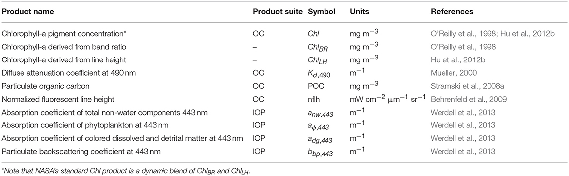
Table 1. Bio-optical ocean color data products.

Modeling Bio-Optical Data Product Uncertainty

In this study we used the analytical law of propagation of uncertainty (JCGM, 2008) to propagate radiometric uncertainties through models used to derive bio-optical quantities. We follow the notation conventions outlined by JCGM (2008) where the uncertainty of a measured quantity, y, is denoted as u(y) and is the positive square root of the variance, u²(y). We note that y is derived from a model, f, of N input quantities, x_i. Following (JCGM, 2008), for uncorrelated input quantities, u²(y) can be calculated as:

$\begin{array}{ll}{u}^2\left(y\right)={\displaystyle \sum _{i=1}^N}{\left(\frac{\partial f}{\partial x_i}\right)}^2{u}^2(x_i)& (2)\end{array}$

where, u(x_i) is the 1-σ uncertainty in the input quantity x_i. For our notation of spectral properties used in ocean color remote sensing, subscripts i correspond to wavelength. In this study, partial derivatives of target parameters were calculated analytically, however, these could also be computed numerically. For the situation where uncertainties of input quantities are correlated, Equation 2 is extended to:

$\begin{array}{ll}{u}^2(y)={\displaystyle \sum _{i=1}^N}{\left(\frac{\partial f}{\partial x_i}\right)}^2{u}^2(x_i)+2{\displaystyle \sum _{i=1}^{N-1}}{\displaystyle \sum _{j=i+1}^N}\frac{\partial f}{x_i}\frac{\partial f}{x_j}u(x_i,x_j)& (3)\end{array}$

where u(x_i, x_j) = u(x_j, x_i) denotes the estimated error covariance associated with the quantities x_i and x_j. Comprehensive details of partial derivative calculations for each bio-optical algorithm in Table 1 are given in Appendices A–E (Supplementary Material).

Monte Carlo (MC) methods are routinely used to perform sensitivity analyses as well as quantify model output uncertainties (Refsgaard et al., 2007). In this study, we have utilized a MC approach to appraise FOFM calculations. As the partial derivative calculus within FOFM uncertainty estimates can be complex, we have used MC-to-FOFM comparisons as a means of checking calculations.

The MC estimates of uncertainties in this study were computed as follows:

(i) A given bio-optical model, f, that derives an output y, that is considered a function of n spectral remote sensing reflectance bands, R_rs,i, is run 5,000 times.

(ii) Upon each iteration, each R_rs,i is perturbed by a factor Δr_,i which is randomly sampled from a Gaussian distribution Δr_,i ~N(0,u(R_rs,i)), in which the mean is zero and the standard deviation, u(R_rs,i), is known or assumed. No spectral correlations are assumed.

(iii) The MC simulation then generates a probability density function (PDF) for y. From the PDF, the mean value, ŷ and the standard deviation, σ_y, can be computed.

We note that the MC method captures non-linear effects and thus we cannot always expect direct agreement between ${\sigma }_y^2$ and FOFM-derived u²(y). Indeed, even if a bio-optical model contains weak non-linearities and MC model input uncertainties are normally distributed, the number of MC iterations still needs to be suitably large for ${\sigma }_y^2$ to agree with u²(y).

Evaluation R_rs Dataset

To evaluate our FOFM uncertainty method, we used a dataset of high quality hyperspectral R_rs,i spectra (N = 1124). Hyperspectral radiometric measurements were collected in situ during three different expeditions, representing a range of oligotrophic to mesotrophic waters: the SABOR experiment in the Gulf of Maine/North Atlantic/Mid-Atlantic coast (July–August 2014); AE1319 in the North Atlantic and Labrador Sea (August–September 2013); and NH1418 in the Equatorial Pacific (September–October 2014). A HyperOCR system (Sea-Bird Scientific) deployed on a tethered profiler in “buoy mode” was used to collect upwelling radiance, L_u,i (W m⁻² μm⁻¹ sr⁻¹), and downwelling irradiance, E_d,i (W m⁻²), spectra during deployments lasting ~5 min. During sample collection, the instrument was allowed to drift far enough from the boat to avoid the ship's shadow.

The spectra were dark and tilt-corrected, and the upper and lower 25th percentile of the E_d,i spectra were removed from both E_d,i and L_u,i. The mean of the remaining spectra was used in subsequent analysis, providing one spectrum per deployment, and with uncertainties calculated as the standard deviation of the same spectra used to calculate the mean (N.B. uncertainties here represent only the experimental portion of the uncertainties, and calibration bias has not been accounted for). The L_u,i measurements were extrapolated to and across the air-water interface to obtain the water-leaving radiance, L_w,i (W m⁻² sr⁻¹), which were then used to calculate remote-sensing reflectance (R_rs,i), defined as:

$\begin{array}{ll}{R}_{rs,i}=\frac{L_{w,i}}{E_{d,i}}& (4)\end{array}$

The spectra were additionally corrected for Raman scattering following methods in Westberry et al. (2013), which was necessary to compensate for the scattering that water molecules themselves can contribute to L_w,i, especially at the blue wavelengths in very clear waters (McKinna et al., 2016). Finally, the R_rs spectra were normalized to remove the angular effect of the sun position in the sky relative to nadir, following methods in Lee et al. (2011). For a more detailed description of the R_rs,i calculations and processing, see Data and Methods section in Chase et al. (2017). All hyperspectral R_rs,i used in this study are shown in Figure 1.

FIGURE 1

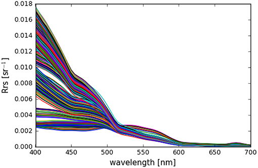
Figure 1. Hyperspectral remote-sensing reflectances (N = 1124) used in this study.

Finally, each hyperspectral R_rs spectrum was spectrally sub-sampled. The resulting multiband R_rs,i dataset had sixteen 10 nm-wide spectral bands centered on: 412, 425, 443, 460, 475, 490, 510, 532, 555, 583, 617, 640, 655, 665, 678, and 710 nm. This multispectral subset spanned the visible domain and included bands from both past and present NASA sensors (e.g., SeaWiFS and MODIS).

Radiometric Uncertainties

Spectrally Flat R_rs Uncertainties

For NASA ocean color bio-optical algorithms, model input quantities are typically remote sensing reflectances, R_rs,i (sr⁻¹), which are derived from measured top-of-atmosphere radiances, L_t,i (W m⁻² μm⁻¹ sr⁻¹), via atmospheric correction (AC) algorithms. Historically, a desirable science requirements for NASA ocean color missions has been R_rs,i with relative uncertainty of 5% (spectrally flat) or less (Hooker et al., 1992; Hooker and McClain, 2000; McClain et al., 2004; PACE Science Definition Team, 2018). Whilst not directly representative of a true sensor (see section Spectrally-Dependent R_rs Uncertainties), treating relative uncertainties in R_rs,i as spectrally flat is still useful under circumstances where detailed knowledge of sensor performance characteristics is limited, such as during pre-launch scoping studies, to provide rudimentary uncertainty estimates. In this study we first consider 5% relative uncertainty in R_rs,i to compare FOFM-to-MC calculations. We next use the FOFM method consider how spectrally flat relative uncertainties in R_rs of 1, 5, and 10% impact estimated OC and IOP uncertainties. Note, we treat spectrally flat relative uncertainties in R_rs of 1, 5, and 10% as spectrally uncorrelated.

Spectrally-Dependent R_rs Uncertainties

We note that on-orbit uncertainties in L_t,i and R_rs,i have previously been quantified for NASA's SeaWiFS and MODISA missions (Eplee et al., 2007; Hu et al., 2012a, 2013; Angal et al., 2015). Whilst historically 5% has been the desired accuracy goal for R_rs in the blue-green spectral range, work by Hu et al. (2013) reported that relative uncertainties of R_rs,i for SeaWiFS and MODISA increase monotonically with wavelength, and that R_rs,i relative uncertainty also varies as a function of Chl, or water-column optical complexity. To extend this study beyond spectrally flat relative uncertainties, we utilized the relative uncertainties for MODISA R_rs,i estimated for the North Atlantic Ocean (see Table 2 of Hu et al., 2013). To estimate relative uncertainty for a given R_rs,i spectra, we followed three steps: (i) linearly interpolate tabulated relative uncertainties to match the spectral resolution of our in situ R_rs,i dataset, (ii) estimate Chl concentration using NASA's standard OC algorithm, and (iii) linearly interpolate the spectrally tabulated relative uncertainties to estimate relative uncertainty for observed R_rs,i based on the respective Chl concentration. Note, where estimated Chl exceeded 0.2 mg m⁻³ [beyond values reported by Hu et al. (2013)] we linearly extrapolated tabulated relative uncertainties. Figure 2 shows the spectral relative uncertainties in R_rs,i [sensu Hu et al. (2013)] used in this study and how they vary with Chl concentration. Note, spectrally-dependent relative uncertainties in R_rs computed as a function of Chl were treated as spectrally uncorrelated.

FIGURE 2

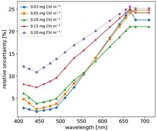
Figure 2. Relative uncertainties of R_rs varying with Chl concentration. Original data taken from Hu et al. (2013) and interpolated to the multispectral resolution used in this study.

Spectrally-Correlated R_rs Uncertainties

Our initial analyses treated R_rs spectral uncertainties as uncorrelated, which in practice is an oversimplification. Indeed, AC algorithms utilize near-infrared bands to make assumptions about the contribution of atmospheric aerosols to L_t (Gordon and Wang, 1994; Bailey et al., 2010). Thus, R_rs,i uncertainties are inherently spectrally correlated. While much work has been done to characterize radiometric uncertainties of NASA sensors used for ocean color (Eplee et al., 2007; Hu et al., 2012a, 2013), few studies have quantified off-diagonal elements of the variance-covariance matrices for top-of-atmosphere radiance, V_Lt, and remote sensing reflectances, V_Rrs, respectively. We note that while beyond the scope of this work, parallel efforts are underway by the research community to derive pixel-by-pixel estimates of u(R_rs,i) by propagating radiometric uncertainties through ocean color atmospheric correction algorithms (Gillis et al., 2018).

Recently, Lamquin et al. (2013) demonstrated a methodology to estimate V_Lt for MERIS data and propagate these through ESA's clear water branch AC algorithm and into bio-optical data products. Critically, Lamquin et al. (2013) demonstrated that ignoring covariances can lead to overestimated data product uncertainties. In this study, using a similar methodology to Lamquin et al. (2013), we estimate V_Lt for SeaWiFS and then using a numerical approximation estimate V_Rrs. A full description of this method can be found in Appendix F (Supplementary Material). We note that while our estimates of V_Rrs are somewhat rudimentary, they are still useful for demonstrating the importance of including covariance terms in FOFM-based uncertainty estimates.

Satellite Data Processing

A SeaWiFS image of Hawaii captured on 1 December 2000 was used to demonstrate the FOFM methodology when applied to ocean color imagery. SeaWiFS Level-1 data was downloaded from NASA's Ocean Biology Distributed Active Archive Center (NASA OB.DAAC) Level 1 and 2 Browser website (https://oceancolor.gsfc.nasa.gov/)¹. Data were then processed from Level 1 to Level 2 using NASA Ocean Color Science Software (OCSSW). These processing steps include radiometric calibration, geolocation, and atmospheric correction. A prototype version of OCSSW code was used to compute u(Chl) using FOFM methodology where u(R_rs,i) was estimated using an empirical methodology described in Appendix F (Supplementary Material).

Results

Appraisal of Methodology

The MC methodology, while computationally expensive, was expected to give robust estimates of measurand uncertainties. Thus, MC outputs provided a benchmark to which the FOFM uncertainty estimates could be compared with for correctness. Direct calculations of FOFM uncertainties, u(y), were compared with MC output uncertainties, σ_y. To compare MC and FOFM calculations we used 5% spectrally flat relative uncertainty in R_rs and computed the following comparison statistics: bias and Type II linear regression slope. When computing these statistics for the purpose of FOFM-to-MC comparisons, we assume that MC-estimated uncertainties were quasi-truth. We note that variables were log-transformed for these calculations following Seegers et al. (2018). Bias was computed as:

$\begin{array}{ll}bias=10^{\wedge }\left\{{\displaystyle \sum _{k=1}^N}\frac{{log}_{10}(M{C}_k)-{log}_{10}(FOF{M}_k)}{N}\right\},& (5)\end{array}$

where N = 1124 is the number of input spectra. Given that bias was computed using log-transformed variables, it becomes interpretable as multiplicative metrics (Seegers et al., 2018). We note that our bias calculations assume estimated OC and IOP uncertainties follow log-normal distributions; a property that is demonstrated later in the paper (e.g., Figures 4, 5).

The MC and FOFM estimation of derived product uncertainties were in good agreement for the following OC products: K_d,490, POC, and nflh. This was indicated by slope and bias and statistics (Table 2) having values of, or near to, 1.0. However, regression statistics indicated Chl uncertainties derived using the FOFM method did not completely agree with the MC method (Table 2). To assess this discrepancy more closely, uncertainties in each component of the Chl algorithm were inspected, namely the band ratio (BR), line height (LH), and blended components. Regression statistics indicated that FOFM estimates of ChL_blend product uncertainties did not agree well with MC values and were typically biased low by 27%, visualized further by the color-coded scatter plot in Figure 3A.

TABLE 2

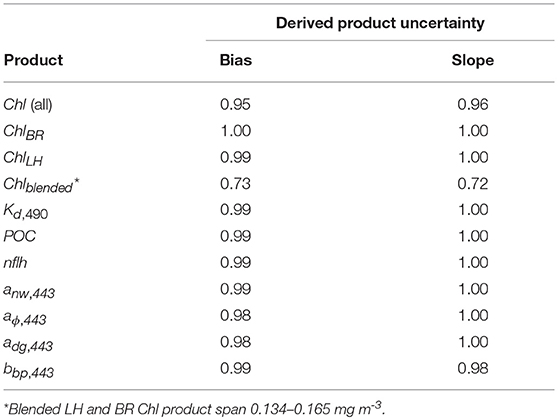
Table 2. Log-normal statistics comparing Monte Carlo (MC) and first-order first-moment (FOFM) uncertainty calculations for R_rs with spectrally flat, uncorrelated 5% relative uncertainty.

FIGURE 3

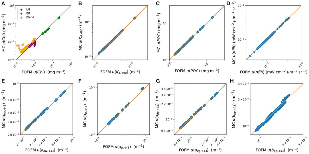
Figure 3. Scatter plot comparisons of data product uncertainties estimated from FOFM with those estimated from Monte Carlo (MC) simulations. (A–D) OC products Chl, K_d,490, POC, and nflh, respectively. Note that the scatter plot of Chl uncertainty is color coded with respect to the method use to derive the output product (line height: purple, band ratio: green, blended: yellow). (E–H) IOP products a_nw,443, a_ϕ,443, a_dg,443, and b_bp,443, respectively.

Derived uncertainties for IOP products generally agreed with MC simulations. Specifically, Table 2 shows FOFM estimates of uncertainties with respect to MC estimates for a_nw,443, a_ϕ,443, a_dg,443, and b_bp,443 were biased low by 1%, low by 2%, low by 2% and, high by 2%, respectively. Slight disagreement between MC and FOFM estimates of u(b_bp,443) can be visualized in Figure 3 when u(b_bp,443) > 2.0 × 10⁻³ m⁻¹. In addition, MC and FOFM estimates of u(a_ϕ,443) showed slight disagreement when u(a_ϕ,443) > 1.0 × 10⁻² m⁻¹.

These results demonstrate that while FOFM uncertainty calculations are computationally inexpensive, they serve as approximations only, especially in the case of Chl. Indeed, while FOFM-derived uncertainties can be expected to agree with MC-derived values for simple functions that vary linearly, it may not be unusual for FOFM-derived uncertainties to differ from MC-derived values; particularly when analyzing complicated non-linear problems (Putko et al., 2001; Mekid and Vaja, 2008). For example, with the IOPs we found slight differences in the order of 1% between MC and FOFM uncertainty estimates. For such mathematical functions, higher order methods such as Second Order First Moment (SOFM) methods may be useful, however, the added mathematical complexity may be prohibitive.

Uncertainties Estimated From in situ Radiometric Data

OC Product Uncertainties

Using the multispectral R_rs evaluation dataset, uncertainties in derived OC products associated with 5% spectrally-flat relative, uncorrelated uncertainty in R_rs were computed. Figure 4 shows histograms of derived OC products, absolute uncertainties, and relative uncertainties. MC computations are summarized in Table 3, while FOFM computations are provided for comparative purposes in Table 4.

FIGURE 4

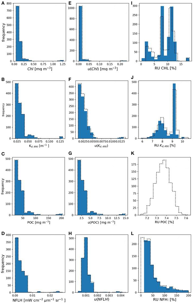
Figure 4. (A–D) Histograms of derived Chl, K_d,490, POC, and nflh, respectively. (E–H) Histograms of FOFM-estimated uncertainties in derived Chl, K_d,490, POC, and nflh, respectively computed using 5% spectrally flat, uncorrelated uncertainty in input R_rs. (I–L) Histograms of FOFM-estimated relative uncertainties in derived Chl, K_d,490, POC, and nflh, respectively. Note: FOFM-estimates of POC relative uncertainties in this example were invariant. Dashed curves represent MC results, solid blue bars represent FOFM results.

TABLE 3

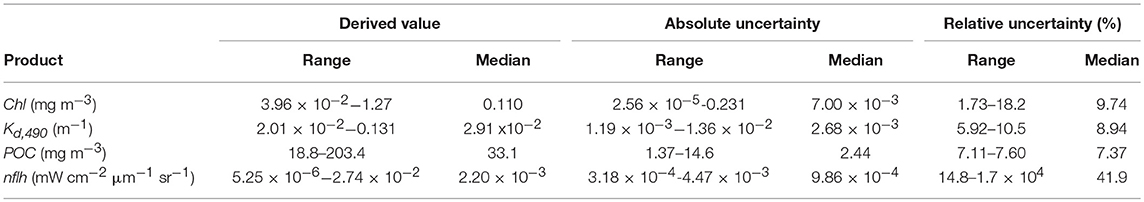
Table 3. OC products and associated uncertainties derived via MC method with 5%, uncorrelated relative uncertainty in R_rs.

TABLE 4

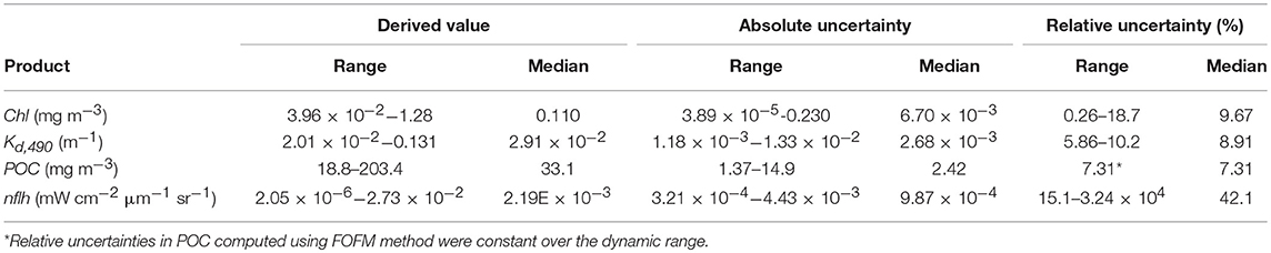
Table 4. OC products and associated uncertainties derived via FOFM method with 5%, uncorrelated relative uncertainty in R_rs.

The range of derived Chl confirmed that the dataset spans oligotrophic (0.04 mg m⁻³) to mesotrophic conditions (1.28 mg m⁻³) with a median value of 0.11 mg m⁻³. Values of u(Chl) span four orders of magnitude and have median values of 7.00 × 10⁻³ and 6.70 × 10⁻³ mg m⁻³ for the MC and FOFM methods, respectively. The relative uncertainties for Chl span a single order of magnitude and have median values of 9.74 and 9.67% for the MC and FOFM methods, respectively. Although the histogram of derived Chl in Figure 4 appears log-normally distributed, two distinct peaks are present; a low peak (ranging from 0 to 0.5 mg m⁻³) and a high peak (centered on 1.1 mg m⁻³). Since bio-optical properties are log-normally distributed in the ocean (Campbell, 1995), the peaks observed in the distributions of derived bio-optical variables are probably due to the limited size of the hyperspectral R_rs dataset (N = 1124), that does not uniformly span the entire range of oceanic conditions (see Figure 1A in Chase et al., 2017).

The range of derived K_d,490 spans an order of magnitude with a median value of 0.0291 m⁻¹. The values of u(K_d,490) also span an order of magnitude with median values of 2.68 × 10⁻³ m⁻¹ for both MC and FOFM calculations. The relative uncertainties for K_d,490 span a single order of magnitude and have a median value of 8.94 and 8.91% for MC and FOFM calculations, respectively. The range of derived POC spans two orders of magnitude with a median value of 33.1 mg m⁻³. The values of u(POC) span an order of magnitude and have median values of 2.44 and 2.42 mg m⁻³ for MC and FOFM calculations, respectively. The relative uncertainties in POC have a value of 7.37 and 7.31% for MC and FOFM calculations, respectively. We note that the relative uncertainty in POC as computed by FOFM method exhibits no spread. For uncorrelated, spectrally flat relative uncertainties, u(POC)/POC is a function of u(R_rs,443)/R_rs,443 and u(R_rs,555)/R_rs,555. Thus, when u(R_rs,443)/R_rs,443 and u(R_rs,555)/R_rs,555 are fixed (e.g., at 5%), u(POC)/POC is fixed. In practice, this will not always hold true, particularly when relative uncertainties in R_rs are variable and spectrally dependent. We note that in Figure 4 the MC-derived relative uncertainties for POC are normally distributed over a narrow range centered on 7.37%.

The range of nflh spans three orders of magnitude with an MC-estimated median value of 2.20 × 10⁻³ mW cm⁻² μm⁻¹ sr⁻¹. We note that direct calculations of nflh resulted in a median value of 2.19 × 10⁻³ mW cm⁻² μm⁻¹ sr⁻¹. The values of u(nflh) span an order of magnitude with median values of 9.86 × 10⁻⁴ and 9.87 × 10⁻⁴ mW cm⁻² μm⁻¹ sr⁻¹ for MC and FOFM calculations, respectively. The median relative uncertainty in nflh was 41.9 and 42.1% for MC and FOFM calculations, respectively (Figure 4). We note that the range of relative errors for nflh is very large (for MC calculations: 14.8–1.7 × 10⁴%), and these should be interpreted with a caution. Low values of nflh, in the order of 1 × 10⁻⁶ mW cm⁻² μm⁻¹ sr⁻¹, were derived from the evaluation dataset which in most likelihood would be beyond the detection limit of existing ocean color sensors. Further, while the absolute uncertainties associated with these low nflh values may also be small in magnitude, they can still manifest as large relative uncertainties.

IOP Product Uncertainties

Using the radiometric evaluation dataset, uncertainties in derived IOP products associated with 5% relative, uncorrelated uncertainty in R_rs,i were computed following the methodology in Appendix E (Supplementary Material). Figure 5 shows histograms of derived IOP products, absolute uncertainties, and relative uncertainties. MC computations are summarized in Table 5 while FOFM computations are provided for comparative purposes in Table 6.

FIGURE 5

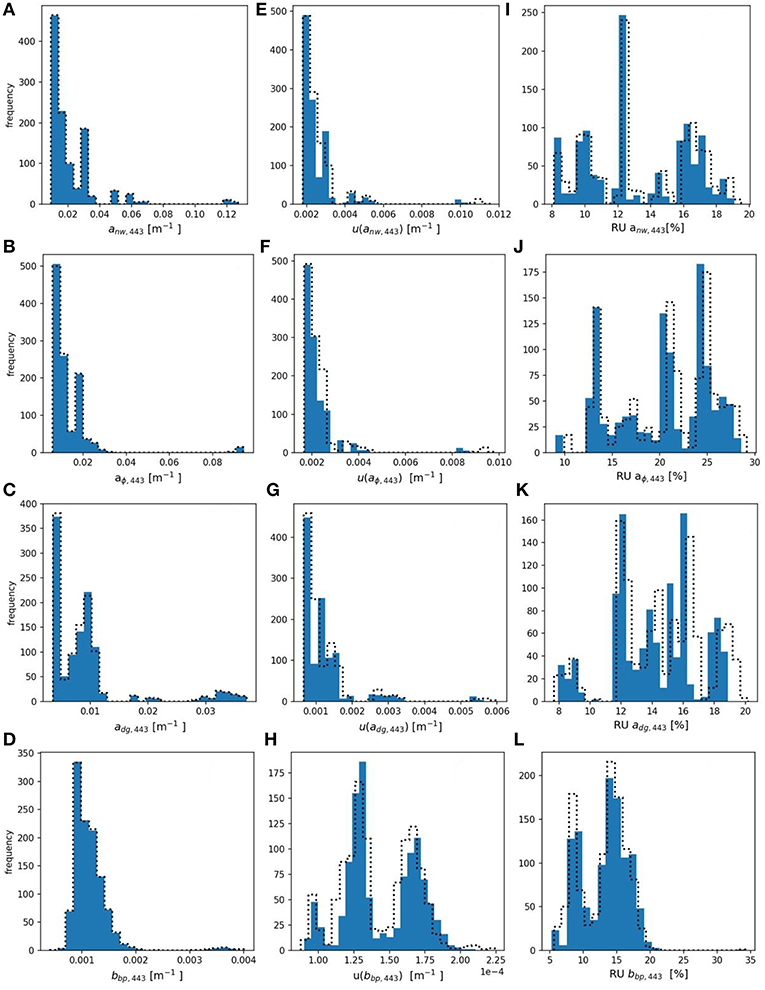
Figure 5. (A–D) histograms of derived a_nw,443, a_dg,443, a_ϕ,443, and b_bp,443, respectively. (E–H) histograms of FOFM-estimated uncertainties in derived a_nw,443, a_dg,443, a_ϕ, 443, and b_bp,443, respectively, computed using 5% spectrally flat, uncorrelated uncertainty in input R_rs. (I–L) histograms of FOFM-estimated relative uncertainties in derived a_nw.443, a_dg,443, a_ϕ,443, and b_bp,443, respectively. Dashed curves represent MC results, solid blue bars represent FOFM results.

TABLE 5

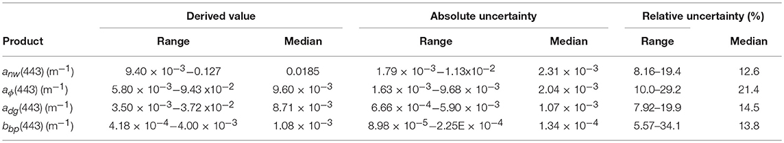
Table 5. IOP products and associated uncertainties derived using MC method with 5%, uncorrelated relative uncertainty in R_rs.

TABLE 6

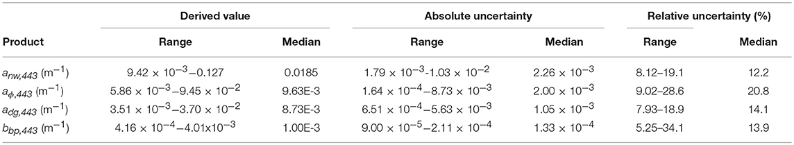
Table 6. IOP products and associated uncertainties derived using FOFM method with 5%, uncorrelated relative uncertainty in R_rs.

The range of derived a_nw,443 spans two orders of magnitude with a median value of 0.0185 m⁻¹. Values of u(a_nw,443) span an order of magnitude with median values of 2.31 × 10⁻³ and 2.26 × 10⁻³ m⁻¹ for MC and FOFM methods, respectively. The median relative uncertainty in a_nw,443 spans a single order of magnitude and has median values of 12.6 and 12.2% for MC and FOFM methods, respectively. The range of a_ϕ,443, a_dg,443, and b_bp,443 all span a single order of magnitude with median values of 9.6 × 10⁻³, 8.71 × 10⁻³, and 1.08 × 10⁻³ m⁻¹, respectively. Absolute uncertainties in IOPs all span two orders of magnitude apart from u(a_ϕ,443) which spanned a single order of magnitude. Highest relative uncertainties of all GIOP-derived products are for a_ϕ,443 (~20%), whereas a_nw,440, a_dg,440, and b_bp,440 have relative uncertainties of similar magnitude that are all <15%.

Summary of MC and FOFM Comparisons

FOFM and MC estimates of OC and IOP uncertainties were generally in good agreement. This provides confidence that our FOFM analytical formulations were correct. However, FOFM-to-MC comparisons of Chl and IOP uncertainties, whilst similar in magnitude, exhibited a degree of scatter around the one-to-one line. We expect that these differences may be due to the MC method's ability to handle non-linearity and discontinuities in the models more robustly than the FOFM approach. For example, the Chl model has several complex features such: switching between ChL_BR and ChL_LH, the ChL_BR model's selection of maximum band ratios, and the blending of ChL_BR and ChL_LH, which may not be fully captured by the FOFM method.

We thus found FOFM-to-MC comparisons to be useful as a “quick acceptability checking” of FOFM calculations. In practice, however, one should not always assume the two methods will closely agree as the MC model may handle non-linearities and discontinuities more robustly than the FOFM method. The FOFM and MC calculations also indicate that for normally distributed radiometric input uncertainties, the estimated output uncertainties for OC and IOP were log-normally distributed (as per Figures 4, 5). Such highly dynamic and variable nature of uncertainties in ocean color data products highlights the need for these estimates to be done on a pixel-by-pixel basis, rather than a single scene-wide estimate, further justifying the need for simplified, computationally inexpensive approach (i.e., FOFM).

We note that our FOFM uncertainty formulation for the GIOP currently does not consider uncertainty in spectral shape models [i.e., u($a_{\varphi ,i}^{*}$) and u($b_{bp,i}^{*}$)]. Indeed, we believe that this may be why there were some noticeable differences when comparing FOFM and MC methods, for example: when u(b_bp,443) > 2.00 × 10⁻⁴ m⁻¹ (Figure 3H). In a cursory study, we re-ran both FOFM and MC calculations with the shape models parametrized as spectral constants (i.e., having no uncertainties). This resulted in improved FOFM-to-MC comparisons (results not shown) and further highlighted how spectral shape uncertainties impact our FOFM uncertainty estimates. As part of future work, we thus plan to extend our current GIOP FOFM uncertainty formulation to include the spectral shape uncertainties. Additionally, we note that u($a_{\varphi ,i}^{*}$) and u($b_{bp,i}^{*}$), computed as functions of Chl and a red-green R_rs,i ratio, respectively, are also correlated. Thus, an improved GIOP FOFM uncertainty formulation should also consider covariances between spectral shape models.

GIOP Model Misfit Uncertainties

In this analysis we used our high-quality evaluation R_rs dataset to approximate GIOP model misfit uncertainties. Our assumptions in this exercise were: (i) the uncertainties in our R_rs dataset are small, and (ii) the least squares residual of the optimal solution (model misfit) are thus due to an imperfect model.

In this analysis we first computed the error-covariance matrix, E_rrs, for each R_rs observation as follows: (i) employ the Levenberg-Marquardt non-linear least squares optimization to iteratively find an optimal solution for the free variables x_ϕ, x_dg, and x_p which correspond to Chl concentration, a_dg,440, and b_bp,440, respectively (see Appendix E in Supplementary Material for further detail). We note that in the standard implementation of the GIOP, the cost function (Chi-squared) is unweighted. (ii) feed the optimal set of x_ϕ, x_dg, and x_p back in the forward reflectance model to compute a best-fit spectral sub-surface remote sensing reflectance, $r_{rs,i}^{\text{mod}}$. (iii) calculate the spectral residual, ε_rrs,i, between $r_{rs,i}^{\text{mod}}$ and sensor-observed subsurface remote sensing reflectance. (iv) set the diagonal elements of E_rrs as the square of ε_rrs,i.

Next, by substituting E_rrs for V_rrs in Equation E13 the parameter error-covariance matrix, E_x, can be computed as:

$\begin{array}{ll}{\text{E}}_{\text{x}}={\text{J}}^{-1}{\text{E}}_{\text{rrs}}{({\text{J}}^{\text{T}})}^{-1}& (6)\end{array}$

Where J is the Jacobian matrix of the forward model (see Appendix E in Supplementary Material for derivation). Finally, the estimates of parameter uncertainties due to model misfit were calculated as the square root of the diagonal elements of E_x. The model-misfit uncertainties are summarized in Table 7 and compared to parameter uncertainties due to Hu spectrally-dependent radiometric uncertainties (as per Table 6).

TABLE 7

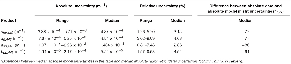
Table 7. GIOP model-misfit uncertainties estimated using the evaluation R_rs dataset.

We found that estimated GIOP model misfit uncertainties were 60–90% smaller than those imparted by radiometric uncertainty. Thus, by combining the two during pixel-by-pixel processing, it would be possible to more completely estimate u_measurement(y) for IOPs. However, we accept that our FOFM model-data misfit approach is approximate only and does not consider all uncertainties in the GIOP model formulation.

Comparing Product Uncertainties Due to Various Radiometric Input Uncertainties

In order to evaluate the impact of different R_rs uncertainty values on derived product uncertainties, using the FOFM method we: (i) propagated spectrally flat, uncorrelated R_rs relative uncertainties of 1, 5, and 10% through OC and IOP models, and (ii) propagated spectrally-dependent, uncorrelated u(R_rs) through OC and IOP models by linearly interpolating/extrapolating tabulated data published by Hu et al. (2013), referred to as “Hu uncertainties” (see Figure 2). Summary results of this analysis are given in Tables 8, 9. As expected, introducing spectrally flat, uncorrelated R_rs uncertainties of lower and higher value than the previously evaluated 5%, resulted in respectively, lower and higher uncertainties in data products, while the distribution of uncertainties kept the same shape as for the 5% run (Figure 6). For the product uncertainties derived using the “Hu R_rs uncertainties,” both the shape of the distribution and median values changed from the 5% run (Figure 6). These results demonstrate the importance of considering spectral dependence in radiometric uncertainties. Notably, considering spectrally flat 5% relative uncertainties in R_rs for a data product such as nflh, which utilizes red-end bands, may result in significant underestimation of likely data product uncertainties.

TABLE 8

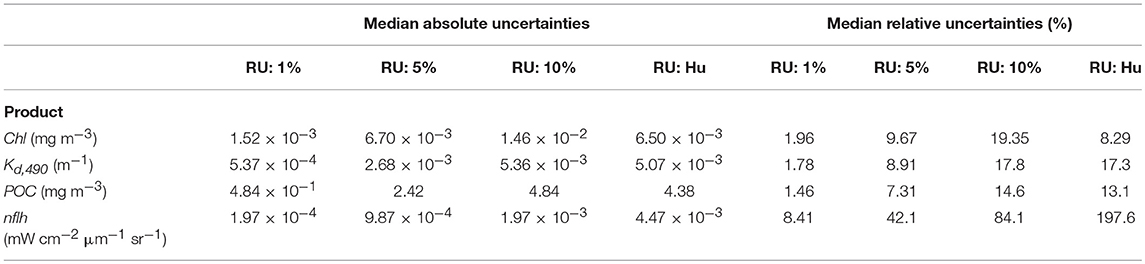
Table 8. Median OC data product uncertainties computed as relative uncertainties (RU) in R_rs vary.

TABLE 9

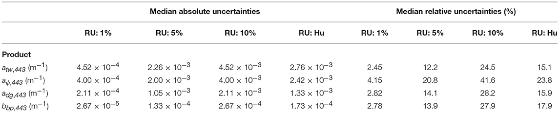
Table 9. Median IOP data product uncertainties computed as relative uncertainties (RU) in R_rs vary.

FIGURE 6

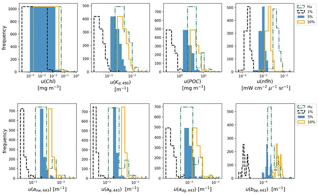
Figure 6. Upper row are histograms of derived OC data products uncertainties estimated using the FOFM method. Bottom row are histograms of derived IOP data product uncertainties estimated using the FOFM method. The four histograms in each subplot correspond to four different input u(R_rs): spectrally flat R_rs relative uncertainties of 1% (dashed black), 5% (blue), and 10% (orange) as well as spectrally dependent relative uncertainties taken from Hu et al. (2013) outlined in green dashed line.

Spectrally flat relative uncertainty in R_rs (e.g., 5% in the blue-green region) is a commonly used accuracy goal for ocean color missions. However, we know from on-orbit data that sensors such as SeaWiFS and MODIS have largely not achieved their desired accuracy goals over the full spectral range (Hu et al., 2013), particularly at red wavelengths. In lieu of any knowledge of a sensor's radiometric uncertainty characteristics (e.g., during design trade studies), one might decide to utilize desired relative radiometric accuracy goals to approximate ocean color data product uncertainties. However, our results have shown spectrally flat (5%) and spectrally-dependent (Hu) relative R_rs uncertainties lead to different estimates of OC and IOP uncertainties. Indeed, for improved uncertainty estimates, we recommend the use of more representative spectrally-dependent u(R_rs)/R_rs, if known.

Application to Satellite Chlorophyll Image

The potential impact that spectrally-correlated uncertainties in R_rs have upon ocean color data product uncertainties was evaluated using a scene of the southern Hawaiian Islands captured on 1 December 2000 (Figure 7). We have estimated on a pixel-by-pixel basis the covariance matrix of remote sensing reflectances, V_Rrs, as per the methodology described in Appendix F (Supplementary Material). Estimates of u(Chl) were then calculated both with- and without the off-diagonal terms in V_Rrs to demonstrate the impact of incorporating covariance terms (if known) when estimating uncertainties.

FIGURE 7

Figure 7. Derived data products for a SeaWiFS image of waters surrounding the Hawaii Islands captured on 1 December 2000. (A) Chl concentration derived using OCI algorithm, (B) u(Chl) computed with covariances included, (C) relative uncertainty in Chl computed with estimated R_rs covariances included, (D) u(Chl) calculated without estimated R_rs covariances included, and (E) relative uncertainty in Chl computed without estimated R_rs covariances included.

The sample SeaWiFS Chl image (Figure 7A) shows that the clearest waters occurred southeast of Island of Hawaii (largest island) with two large eddies to the west. Regions of elevated Chl concentration are also visible along the northeast coast of the Island of Hawaii, and also adjacent to coastal waters of four islands (Maui, Lanai, Molokai, and Kahoolawe) to the northwest of Hawaii. Derived ChL_blend ranges from 1.83 × 10⁻³ to 0.498 mg m⁻³ with a median of 0.066 mg m⁻³. When the off-diagonal terms in V_Rrs were considered, the estimated values of u(Chl) ranged from 1.30 × 10⁻³ to 0.075 mg m⁻³ with a scene-wide median of 5.20 × 10⁻³ mg m⁻³ (Figure 7B) and the relative uncertainties spanned 0.84–38.6% with a median of 7.89% (Figure 7C). When the off-diagonal terms in V_Rrs were not considered (i.e., set to zero), estimated values of u(Chl) ranged from 1.30 × 10⁻³ to 0.109 mg m⁻³ with a scene-wide median of 5.50 × 10⁻³ mg m⁻³ (Figure 7D) and relative uncertainties spanning 0.85–46.1 % with a median of 8.27% (Figure 7E). Note, these image statistics were computed with standard NASA level-2 quality control flags applied to remove the effect of: land, clouds, sun glint, atmospheric correction failure, product failure, and straylight contamination.

These results demonstrate how a FOFM method can be utilized in operational processing code to estimate uncertainties in derived bio-optical data products. The FOFM method was straightforward to implement within l2gen code and did not add any appreciable processing overhead. Whilst our estimation of V_Rrs is rudimentary (Appendix F in Supplementary Material), it allowed us to consider the covariance terms in the FOFM derivation of u(Chl). Critically, we demonstrated that the inclusion of off-diagonal covariance terms from V_Rrs led to lower estimates of both u(Chl) and u(Chl)/Chl when compared to the same calculations performed with off-diagonal elements of V_Rrs set to zero; a result consistent with findings of Lamquin et al. (2013). Additionally, this example was done with an operational processing code, demonstrating the easiness of implementing a FOFM method within day-to-day ocean color processing.

POC Algorithm Case Study

Recall from Equation 1, we broadly defined measurement uncertainty as having two sources: data uncertainty and model uncertainty. Throughout this paper we have focused heavily on deriving data uncertainties (i.e., propagation of radiometric uncertainty) which is useful if one is trying understand how a specific sensor's noise characteristics may impact derived data product uncertainties. However, this information alone does not provide a complete picture of measurement uncertainty; model uncertainty also needs to be considered. We thus wish to demonstrate how with knowledge of model uncertainties one can draw more complete conclusions about biogeochemically-relevant data product uncertainties. As such, we present a case study in which we estimate POC measurement uncertainty for two different algorithms: (i) Stramski et al. (2008a) and (ii) Rasse et al. (2017).

Our motivation here is to solely demonstrate how one might develop algorithm uncertainty budgets (data and model uncertainty as per Equation 1) using a FOFM framework. Our calculations, however, are limited by: (i) the representativeness of our in situ R_rs dataset which does not encompass all optical water-types found in the World's oceans, (ii) our spectral u(R_rs) values which are estimated from data published by Hu et al. (2013) for a MODIS-like sensor without co-variance terms, and (iii) our knowledge of model uncertainties, such as coefficients uncertainties, which is limited to those reported in literature and/or our best-guess estimates. We hence caution the reader should not use our reported numbers as a basis for algorithm selection.

POC Measurement Uncertainty Estimates

In this exercise, we performed rudimentary calculations to estimate measurement uncertainty budgets for two POC algorithms: (i) NASA's standard POC algorithm (Stramski et al., 2008a) and (ii) the IOP-based model of Rasse et al. (2017). Conveniently for this exercise, both POC models have a power law formulation:

$\begin{array}{ll}POC=a_{poc}{X}^{b_{poc}}& (7)\end{array}$

where X in Stramski et al. (2008a) is a blue-to-green reflectance ratio (R_{rs, 443}/R_rs,555, as per Appendix C in Supplementary Material) and the coefficients a_poc and b_poc have the values of 203.2 and −1.034, respectively. For the approach of Rasse et al. (2017) X is b_bp,₄₇₀ and the coefficients a_poc and b_poc have the values of 141,253 and 1.18, respectively. Note, in this case study we use GIOP-derived estimates of b_bp,₄₇₀ as inputs to the Rasse et al. (2017) model.

First, let us consider the model uncertainty component due to imperfect model coefficients. For both POC algorithms, with the coefficients a_poc and b_poc and their assigned uncertainties of u_model(a_poc) and u_model(b_poc), respectively, we can estimate the model variance for POC as:

$\begin{array}{l}{u}_{\text{model}}^2(POC)={\left(X^{b_{poc}}\right)}^2{u}_{\text{model}}^2(a_{poc})\\ +{\left(a_{poc}{X}^{b_{poc}}log(X)\right)}^2{u}_{\text{model}}^2(b_{poc})\\ +{\left(a_{poc}{b}_{poc}{X}^{b_{poc}-1}\right)}^2{u}_{\text{model}}^2(X)& (8)\end{array}$

In the third term on the right-hand side of Equation 8, we set u_model(X) = 0 and u_model(X) = u_model(b_{bp, 470}) for Stramski et al. (2008a) and Rasse et al. (2017), respectively. We have also assumed the covariance of the coefficients a_poc and b_poc, which are determined by regression fit, is zero. For the Rasse et al. (2017) model, the reported model coefficient uncertainties u_model(a_poc) and u_model(b_poc) are 45,534 and 0.046, respectively. For the Stramski et al. (2008a) model, values of u_model(a_poc) and u_model(b_poc) were not reported. We did, however, estimate these model uncertainties by reanalyzing the original published dataset (Stramski et al., 2008b) and considering the likely uncertainty introduced by not accounting for the effect of filter pad absorption of POC (Novak et al., 2018). Following this cursory analysis (results not shown), we estimated u_model(a_poc) and u_model(b_poc) for the Stramski et al. (2008a) model to be ~2.20 and 0.015, respectively.

Next, we considered the data uncertainty component. The Stramski et al. (2008a) model's data uncertainty FOFM calculus was formulated in Appendix C (Supplementary Material). For the Rasse et al. (2017) model, we first estimated u_data(b_bp,₄₇₀). To do so, b_bp,₄₇₀ was calculated from GIOP-derived b_bp,₄₄₀ as:

$\begin{array}{ll}{b}_{bp,470}=b_{bp,440}\times {\left(\frac{440}{470}\right)}^{\gamma }& (9)\end{array}$

The variance in b_bp,₄₇₀ due to data uncertainty was then estimated as:

$\begin{array}{l}{u}_{data}^2(b_{bp,470})={\left(\frac{\partial b_{bp,470}}{\partial b_{bp,440}}\right)}^2{u}_{data}^2(b_{bp,440})+{\left(\frac{\partial b_{bp,470}}{\partial \gamma }\right)}^2{u}_{data}^2(\gamma )\\ +2\frac{\partial b_{bp,470}}{\partial b_{bp,440}}\frac{\partial b_{bp,470}}{\partial \gamma }{u}_{data}^2(b_{bp,440},\gamma )& (10)\end{array}$

For this exercise, we used GIOP-derived values of u_data(b_bp,₄₇₀) and u(γ). The correlation between derived values of b_bp,547 and γ was used to estimate the covariance term u(b_bp,₅₄₇, γ) as −1.64 × 10⁻⁶ m⁻¹ nm⁻¹. Using, the GUM methodology the variance in the Rasse et al. (2017) POC model due to data uncertainty was then estimated as:

$\begin{array}{ll}{u}_{data}^2(POC)={\left(a_{poc}{b}_{poc}{(b_{bp,470})}^{b_{poc}-1}\right)}^2{u}_{data}^2(b_{bp,470})& (11)\end{array}$

We finally estimated the measurement uncertainty budgets for both POC models using our R_rs evaluation dataset and with Hu spectrally-dependent, uncorrelated radiometric uncertainties (results are shown in Table 10).

TABLE 10

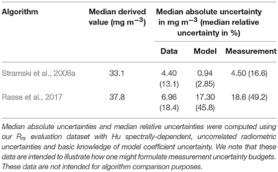
Table 10. Simplified random uncertainty budgets for two POC models.

In our rudimentary measurement uncertainty budget for the Stramski et al. (2008a) POC algorithm, we found the contribution of data (radiometric) uncertainty was larger than model uncertainty. Conversely, for the Rasse et al. (2017) POC algorithm, the contribution of model uncertainty was larger than data uncertainty. Whilst these POC algorithm uncertainty budgets may not be fully representative due to the assumptions we partook here, the exercise nonetheless demonstrates an important point: data and model uncertainties should both be considered if one wishes to use uncertainties as a means of benchmarking/comparing ocean color algorithms.

From an algorithm development perspective one can also use FOFM method to explore the relative contribution of individual uncertainty sources to the combined measurement uncertainty. We have graphically displayed the estimated component uncertainty contribution for each POC algorithm using pie charts (Figure 8). Such information may assist algorithm designers identify and minimize uncertainty sources within a model.

FIGURE 8

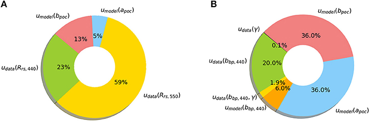
Figure 8. Pie charts demonstrate how individual uncertainty sources contribute to estimates of total measurement uncertainty. Here we consider: (A) a blue-green band-ratio POC algorithm and (B) an IOP-based POC algorithm. We note that these examples are intended to illustrate how one might visualize source contributions to measurement uncertainty. These plots are not intended for algorithm comparison purposes.

Summary of POC Case Study

Our brief example demonstrates the benefits of using the FOFM method for analytically estimating measurement uncertainty in POC. From an ecological perspective, this is particularly useful if one is trying to understand the variability in observed patterns, and distinguish real change from variation in uncertainty. Additionally, it allows for sensitivity analysis, thereby providing a guideline for improving model parameterization. The case study demonstrates how an uncertainty budget can provide additional information to end-users regarding data product quality, potentially informing algorithm selection, and/or guiding new algorithm development. Although ocean color algorithms are typically benchmarked based upon validation matchup metrics (Seegers et al., 2018), we expect model selection and development may be better guided by considering how data and model uncertainties manifest in derived data products.

This case study highlights a challenge if one wishes to compare/benchmark legacy ocean color algorithms based on their measurement uncertainty; one must have reasonable and complete knowledge of both data and model uncertainties to do so. Whilst we have demonstrated that it is possible to estimate and propagate random radiometric uncertainties using the FOFM framework, estimating model uncertainties remains a challenge. This is because model component uncertainties (e.g., model coefficient uncertainties) of legacy ocean color algorithms were not routinely reported. To address this, re-analysis of the structure of legacy ocean color algorithms using high quality bio-optical datasets, such as NASA's bio-Optical Marine Algorithm Dataset (NOMAD; Werdell and Bailey, 2005), may be necessary. Without such knowledge, it remains a challenge to formulate complete measurement uncertainty budgets for legacy ocean color algorithms.

Conclusions

In this paper we demonstrated a FOFM-based method for estimating uncertainties in a selection of NASA OC and IOP products, namely: Chl, K_d,490, POC, nflh, a_nw,440, a_ϕ,440, a_dg,440, and b_bp,440, due to sensor-observed radiometric uncertainty. Using a high quality hyperspectral R_rs dataset subsampled to our target wavelengths, we first appraised the FOFM methodology by comparing FOFM-derived uncertainty estimates with uncertainties estimated from MC simulations with an assumed relative spectrally flat, uncorrelated uncertainty in R_rs of 5%. Our analyses showed that OC and IOP uncertainties estimated using the FOFM method generally agreed with MC simulations. Collectively, the FOFM-to-MC comparisons provided a basis for checking the correctness of the FOFM formulations, which are often algebraically complex. Further, we demonstrated that the FOFM formulation, which is computationally inexpensive, can be applied in routine pixel-by-pixel data processing for estimating uncertainties in derived ocean color data products.

This paper has primarily focused on propagating radiometric uncertainties through bio-optical models (u_data(y) in Equation 1). In practice, the combined measurement uncertainty in derived ocean color data products is expected to be larger once model uncertainties are included. In this study, we have broadly assumed that coefficients within the bio-optical algorithms themselves are errorless, which is not the case. Indeed, most coefficients in bio-optical algorithms have been derived empirically using in situ oceanographic datasets, which themselves have inherent uncertainties due to measurement method and environmental variability. The GIOP, for example, makes assumptions about spectral shapes of IOPs, utilizes an approximate forward reflectance model (Gordon et al., 1988), and employs a model to convert R_rs,_i to R_rs,i (Lee et al., 2002). Thus, there are a number of GIOP model components whose uncertainties, if characterized, may improve the overall estimate of IOP measurement uncertainty. Our case study of POC algorithms also highlighted how the addition of model (e.g., coefficient) uncertainties can further inform end-users, and may potentially guide algorithm development and/or selection.

Although this work represents a first step toward implementing pixel-by-pixel uncertainty estimates in NASA operational ocean color processing code, we recognize that continued effort is required. For example, strategies for quantifying uncertainties in look-up-table (LUT) based models, such as the two-band particulate inorganic carbon (PIC) algorithm (Balch et al., 2005) and bidirectional reflectance distribution function (BRDF) correction (Morel et al., 2002), are needed. Globally, there are a multitude of ocean color algorithms maintained by various researchers and/or institutes and formulating uncertainty estimates must be a collective effort. While the community continues to innovate new bio-optical algorithms, we strongly encourage model developers to characterize uncertainties as a matter of routine.

As we enter the hyperspectral world of PACE, it is credible to expect an evolutionary leap in remote sensing observation of ocean processes detailing, for example, phytoplankton diversity, physiological preferences, and ecology from space. This, parallel to the increase in computational power of the day-to-day data processing, will allow for more complex algorithms; algorithms which will need detailed evaluation of uncertainty budgets, to understand what is real, and what is hidden under the dashed line.

Author Contributions

LM, IC, and PW: conceptualization, methodology, simulations, and data analysis. AC and IC: hyperspectral dataset. LM, IC, PW, and AC: original draft, reviewing, and editing.

Funding

This research was funded by the National Aeronautics and Space Administration (NASA) Ocean Biology and Biogeochemistry Program via an award under the solicitation The Science of Terra, Aqua, and Suomi NPP, Ocean Biology and Biogeochemistry (NNX13AC42G), and PACE mission.

Conflict of Interest Statement

LM was employed by company Go2Q Pty Ltd. The remaining authors declare that the research was conducted in the absence of any commercial or financial relationships that could be construed as a potential conflict of interest.

Acknowledgments

Many thanks to NASA Ocean Biology Processing Group staff for their advice during the preparation of this manuscript. The authors are thankful for all the scientists that contributed to collection of this dataset, especially Wayne Slade and Nicole Poulton, and captains and crews of the UNOLS research vessels. We are also very grateful to the two reviewers for their detailed and insightful comments which have greatly improved this work.

Supplementary Material

The Supplementary Material for this article can be found online at: https://www.frontiersin.org/articles/10.3389/feart.2019.00176/full#supplementary-material

Footnotes

1. ^NASA Goddard Space Flight Center, Ocean Ecology Laboratory, & Ocean Biology Processing Group. Sea-viewing Wide Field-of-view Sensor (SeaWiFS) L1 Data (data/10.5067/ORBVIEW-2/SEAWIFS/L1/DATA/1).

References

Angal, A., Xiong, X., Sun, J., and Geng, X. (2015). On-orbit noise characterization of MODIS reflective solar bands. J. Appl. Remote Sens. 9:094092.

Google Scholar

Antoine, D., d'Ortenzio, F., Hooker, S. B., Bécu, G., Gentili, B., Tailliez, D., et al. (2008). Assessment of uncertainty in the ocean reflectance determined by three satellite ocean color sensors (MERIS, SeaWiFS and MODIS-A) at an offshore site in the Mediterranean Sea (BOUSSOLE project). J. Geophys. Res. Oceans 113, 1–22. doi: 10.1029/2007JC004472

CrossRef Full Text | Google Scholar

Bailey, S. W., Franz, B. A., and Werdell, P. J. (2010). Estimation of near-infrared water-leaving reflectance for satellite ocean color data processing. Opt. Express 18, 7521–7527. doi: 10.1364/OE.18.007521

PubMed Abstract | CrossRef Full Text | Google Scholar

Bailey, S. W., and Werdell, P. J. (2006). A multi-sensor approach for the on-orbit validation of ocean color satellite data products. Remote Sens. Environ. 102, 12–23. doi: 10.1016/j.rse.2006.01.015

CrossRef Full Text | Google Scholar

Balch, W. M., Gordon, H. R., Bowler, B. C., Drapeau, D. T., and Booth, E. S. (2005). Calcium carbonate measurements in the surface global ocean based on Moderate-Resolution Imaging Spectroradiometer data. J. Geophys. Res. Oceans 110, 1–21. doi: 10.1029/2004JC002560

CrossRef Full Text | Google Scholar

Behrenfeld, M. J., Westberry, T. K., Boss, E. S., O'Malley, R. T., Siegel, D. A., Wiggert, J. D., et al. (2009). Satellite-detected fluorescence reveals global physiology of ocean phytoplankton. Biogeosciences 6, 779–794. doi: 10.5194/bg-6-779-2009

CrossRef Full Text | Google Scholar

Campbell, J. W. (1995). The lognormal distribution as a model for bio-optical variability in the sea. J. Geophys. Res. Oceans 100, 13237–13254. doi: 10.1029/95JC00458

CrossRef Full Text | Google Scholar

Chase, A. P., Boss, E., Cetinić, I., and Slade, W. (2017). Estimation of phytoplankton accessory pigments from hyperspectral reflectance spectra: toward a global algorithm. J. Geophys. Res. Oceans 122, 9725–9743. doi: 10.1002/2017JC012859

CrossRef Full Text | Google Scholar

Eplee, J. R. E., Patt, F. S., Barnes, R. A., and McClain, C. R. (2007). SeaWiFS long-term solar diffuser reflectance and sensor noise analyses. Appl. Opt. 46, 762–773. doi: 10.1364/AO.46.000762

PubMed Abstract | CrossRef Full Text | Google Scholar

Franz, B. A., Behrenfeld, M. J., Siegel, D. A., and Signorini, S. R. (2017). Global ocean phytoplankton [in: State of the Climate in 2016]. Bull. Amer. Meteor. Soc. 99, S94–S96. doi: 10.1175/2018BAMSStateoftheClimate.1

CrossRef Full Text | Google Scholar

Gillis, D. B., Bowles, J. H., Montes, M. J., and Moses, W. J. (2018). Propagation of sensor noise in oceanic hyperspectral remote sensing. Opt. Express 26, A818–A831. doi: 10.1364/OE.26.00A818

PubMed Abstract | CrossRef Full Text | Google Scholar

Gordon, H. R., Brown, O. B., Evans, R. H., Brown, J. W., Smith, R. C., Baker, K. S., et al. (1988). A semianalytic radiance model of ocean color. J. Geophys. Res. Atmos. 93, 10909–10924. doi: 10.1029/JD093iD09p10909

CrossRef Full Text | Google Scholar

Gordon, H. R., and Wang, M. (1994). Retrieval of water-leaving radiance and aerosol optical thickness over the oceans with SeaWiFS: a preliminary algorithm. Appl. Opt. 33, 443–452. doi: 10.1364/AO.33.000443

PubMed Abstract | CrossRef Full Text | Google Scholar

Gould, W. G., McCarthy, S. E., Coelho, E., Shulman, I., and Richman, J. G. (2014). Combining satellite ocean color and hydrodynamic model uncertainties in bio-optical forecasts. J. Appl. Remote Sens. 8:083652 doi: 10.1117/1.JRS.8.083652

CrossRef Full Text | Google Scholar

Hooker, S. B., Esaias, W. E., Feldman, G. C., Gregg, W. W., and McClain, C. R. (1992). An Overview of SeaWiFS and Ocean-Color, NASA Tech. Memo. 104566, Vol. 1, eds S. B. Hooker, and E. R. Firestone. Greenbelt, MD: NASA Goddard Space Flight Center, 24.

Google Scholar

Hooker, S. B., and McClain, C. R. (2000). The calibration and validation of SeaWiFS data. Prog. Oceanogr. 45, 427–465. doi: 10.1016/S0079-6611(00)00012-4

CrossRef Full Text | Google Scholar

Hu, C., Feng, L., and Lee, Z. (2013). Uncertainties of SeaWiFS and MODIS remote sensing reflectance: implications from clear water measurements. Remote Sens. Environ. 133, 168–182. doi: 10.1016/j.rse.2013.02.012

CrossRef Full Text | Google Scholar

Hu, C., Feng, L., Lee, Z., Davis, C. O., Mannino, A., McClain, C. R., et al. (2012a). Dynamic range and sensitivity requirements of satellite ocean color sensors: learning from the past. Appl. Opt. 51, 6045–6062. doi: 10.1364/AO.51.006045

PubMed Abstract | CrossRef Full Text | Google Scholar

Hu, C., Lee, Z., and Franz, B. (2012b). Chlorophyll a algorithms for oligotrophic oceans: a novel approach based on three-band reflectance difference. J. Geophys. Res. Oceans 117(C1), 1–25. doi: 10.1029/2011JC007395

CrossRef Full Text | Google Scholar

IOCCG (2008). Why Ocean Colour? The Societal Benefits of Ocean- Colour Technology, Vol. 7. Dartmouthn, NS: IOCCG.

Google Scholar

Jay, S., Guillaume, M., Chami, M., Minghelli, A., Deville, Y., Lafrance, B., et al. (2018). Predicting minimum uncertainties in the inversion of ocean color geophysical parameters based on Cramer-Rao bounds. Opt. Express 26, A1–A18. doi: 10.1364/OE.26.0000A1

PubMed Abstract | CrossRef Full Text | Google Scholar

JCGM (2008). Evaluation of Measurement Data - Guide to the Expression of Uncertainty in Measurement. JCGM 100:2008.

Google Scholar

Lamquin, N., Mangin, A., Mazeran, C., Bourg, B., Bruniquel, V., and D'Andon, O. F. (2013). OLCI L2 Pixel-by-Pixel Uncertainty Propagation in OLCI Clean Water Branch. ESA ATBD ref. S3-L2-SD-01-C01-ACR-TN.

Google Scholar

Lee, Z., Arnone, R., Hu, C., Werdell, P. J., and Lubac, B. (2010). Uncertainties of optical parameters and their propagations in an analytical ocean color inversion algorithm. Appl. Opt. 49, 369–381. doi: 10.1364/AO.49.000369

PubMed Abstract | CrossRef Full Text | Google Scholar

Lee, Z., Carder, K. L., and Arnone, R. A. (2002). Deriving inherent optical properties from water color: a multiband quasi-analytical algorithm for optically deep waters. Appl. Opt. 41, 5755–5772. doi: 10.1364/AO.41.005755

PubMed Abstract | CrossRef Full Text | Google Scholar

Lee, Z., Du, K., Voss, K. J., Zibordi, G., Lubac, B., Arnone, R., et al. (2011). An inherent-optical-property-centered approach to correct the angular effects in water-leaving radiance. Appl. Opt. 50, 3155–3167. doi: 10.1364/AO.50.003155

PubMed Abstract | CrossRef Full Text | Google Scholar

Maritorena, S., d'Andon, O. H. F., Mangin, A., and Siegel, D. A. (2010). Merged satellite ocean color data products using a bio-optical model: characteristics, benefits and issues. Remote Sens. Environ. 114, 1791–1804. doi: 10.1016/j.rse.2010.04.002

CrossRef Full Text | Google Scholar

McClain, C. R. (2009). A decade of satellite ocean color observations. Ann. Rev. Mar. Sci. 1, 19–42. doi: 10.1146/annurev.marine.010908.163650

PubMed Abstract | CrossRef Full Text | Google Scholar

McClain, C. R., Feldman, G. C., and Hooker, S. B. (2004). An overview of the SeaWiFS project and strategies for producing a climate research quality global ocean bio-optical time series. Deep Sea Res. Part II Topical Stud. Oceanogr. 51, 5–42. doi: 10.1016/j.dsr2.2003.11.001

CrossRef Full Text | Google Scholar

McKinna, L. I. W., Werdell, P. J., and Proctor, C. W. (2016). Implementation of an analytical Raman scattering correction for satellite ocean-color processing. Opt. Express 24, A1123–A1137. doi: 10.1364/OE.24.0A1123

PubMed Abstract | CrossRef Full Text | Google Scholar

Mekid, S., and Vaja, D. (2008). Propagation of uncertainty: expressions of second and third order uncertainty with third and fourth moments. Measurement 41, 600–609. doi: 10.1016/j.measurement.2007.07.004

CrossRef Full Text | Google Scholar

Melin, F. (2010). Global distribution of the random uncertainty associated with satellite-derived Chl a. IEEE Geosci. Remote Sens. Lett. 7, 220–224. doi: 10.1109/LGRS.2009.2031825

CrossRef Full Text | Google Scholar

Mélin, F., Sclep, G., Jackson, T., and Sathyendranath, S. (2016). Uncertainty estimates of remote sensing reflectance derived from comparison of ocean color satellite data sets. Remote Sens. Environ. 177, 107–124. doi: 10.1016/j.rse.2016.02.014

CrossRef Full Text | Google Scholar

Moore, T. S., Campbell, J. W., and Dowell, M. D. (2009). A class-based approach to characterizing and mapping the uncertainty of the MODIS ocean chlorophyll product. Remote Sens. Environ. 113, 2424–2430. doi: 10.1016/j.rse.2009.07.016

CrossRef Full Text | Google Scholar

Morel, A., Antoine, D., and Gentili, B. (2002). Bidirectional reflectance of oceanic waters: accounting for Raman emission and varying particle scattering phase function. Appl. Opt. 41, 6289–6306. doi: 10.1364/AO.41.006289

PubMed Abstract | CrossRef Full Text | Google Scholar

Mueller, J. L. (2000). “SeaWiFS algorithm for the diffuse attenuation coefficient, K(490), using water-leaving radiances at 490 and 555 nm,” in eds S. B. Hooker and E. Firestone, R NASA Technical Memorandum 2000-206829, Vol. 11 (Greenbelt, MD: NASA Goddard Space Flight Center), 51.

Google Scholar

Neukermans, G., Ruddick, K., Bernard, E., Ramon, D., Nechad, B., and Deschamps, P.-Y. (2009). Mapping total suspended matter from geostationary satellites: a feasibility study with SEVIRI in the Southern North Sea. Opt. Express 17, 14029–14052. doi: 10.1364/OE.17.014029

PubMed Abstract | CrossRef Full Text | Google Scholar

Novak, M. G., Cetinić, I., Chaves, J. E., and Mannino, A. (2018). The adsorption of dissolved organic carbon onto glass fiber filters and its effect on the measurement of particulate organic carbon: a laboratory and modeling exercise. Limnol. Oceanogr. Methods 16, 356–366. doi: 10.1002/lom3.10248

PubMed Abstract | CrossRef Full Text | Google Scholar

O'Reilly, J. E., Maritorena, S., Mitchell, B. G., Siegel, D. A., Carder, K. L., Garver, S. A., et al. (1998). Ocean color chlorophyll algorithms for SeaWiFS. J. Geophys. Res. Oceans 103, 24937–24953. doi: 10.1029/98JC02160

CrossRef Full Text | Google Scholar

PACE Science Definition Team (2018). Pre-Aerosol, Clouds, and ocean Ecosystem (PACE) Mission Science Definition Team Report. Greenbelt, MD.

Google Scholar

Putko, M. M., Taylor, I. I. I. A. C., Newman, P. A., and Green, L. L. (2001). Approach for input uncertainty propagation and robust design in CFD using sensitivity derivatives. J. Fluids Eng. 124, 60–69. doi: 10.1115/1.1446068

CrossRef Full Text | Google Scholar

Qi, L., Lee, Z., Hu, C., and Wang, M. (2017). Requirement of minimal signal-to-noise ratios of ocean color sensors and uncertainties of ocean color products. J. Geophys. Res. Oceans 122, 2595–2611. doi: 10.1002/2016JC012558

CrossRef Full Text | Google Scholar

Rasse, R., Dall'Olmo, G., Graff, J., Westberry, T. K., van Dongen-Vogels, V., and Behrenfeld, M. J. (2017). Evaluating optical proxies of particulate organic carbon across the surface atlantic ocean. Front. Marine Sci. 4, 1–18. doi: 10.3389/fmars.2017.00367

CrossRef Full Text | Google Scholar

Refsgaard, J. C., van der Sluijs, J. P., Højberg, A. L., and Vanrolleghem, P. A. (2007). Uncertainty in the environmental modelling process – a framework and guidance. Environ. Model. Softw. 22, 1543–1556. doi: 10.1016/j.envsoft.2007.02.004

CrossRef Full Text | Google Scholar

Salama, M. S., Dekker, A., Su, Z., Mannaerts, C. M., and Verhoef, W. (2009). Deriving inherent optical properties and associated inversion-uncertainties in the Dutch Lakes. Hydrol. Earth Syst. Sci. 13, 1113–1121. doi: 10.5194/hess-13-1113-2009

CrossRef Full Text | Google Scholar

Salama, M. S., Mélin, F., and Van der Velde, R. (2011). Ensemble uncertainty of inherent optical properties. Opt. Express 19, 16772–16783. doi: 10.1364/OE.19.016772

PubMed Abstract | CrossRef Full Text | Google Scholar

Seegers, B. N., Stumpf, R. P., Schaeffer, B. A., Loftin, K. A., and Werdell, P. J. (2018). Performance metrics for the assessment of satellite data products: an ocean color case study. Opt. Express 26, 7404–7422. doi: 10.1364/OE.26.007404

PubMed Abstract | CrossRef Full Text | Google Scholar

Stramski, D., Reynolds, R. A., Babin, M., Kaczmarek, S., Lewis, M. R., Rottgers, R., et al. (2008a). Relationships between the surface concentration of particulate organic carbon and optical properties in the eastern South Pacific and eastern Atlantic Oceans. Biogeosciences 5, 171–201. doi: 10.5194/bg-5-171-2008

CrossRef Full Text | Google Scholar

Stramski, D., Reynolds, R. A., Babin, M., Kaczmarek, S., Lewis, M. R., Röttgers, R., et al. (2008b). Concentration of particulate organic carbon and optical properties in the eastern South Pacific and eastern Atlantic Oceans. Supplement to: Stramski, D et al. (2008): Relationships between the surface concentration of particulate organic carbon and optical properties in the eastern South Pacific and eastern Atlantic Oceans. Biogeosciences 5, 171–201. doi: 10.5194/bg-5-171-2008

CrossRef Full Text | Google Scholar

Wang, P., Boss, E. S., and Roesler, C. (2005). Uncertainties of inherent optical properties obtained from semianalytical inversions of ocean color. Appl. Opt. 44, 4074–4085. doi: 10.1364/AO.44.004074

PubMed Abstract | CrossRef Full Text | Google Scholar

Werdell, P. J., and Bailey, S. W. (2005). An improved in-situ bio-optical data set for ocean color algorithm development and satellite data product validation. Remote Sens. Environ. 98, 122–140. doi: 10.1016/j.rse.2005.07.001

CrossRef Full Text | Google Scholar

Werdell, P. J., Franz, B. A., Bailey, S. W., Feldman, G. C., Boss, E., Brando, V. E., et al. (2013). Generalized ocean color inversion model for retrieving marine inherent optical properties. Appl. Opt. 52, 2019–2037. doi: 10.1364/AO.52.002019

PubMed Abstract | CrossRef Full Text | Google Scholar

Westberry, T. K., Boss, E., and Lee, Z. (2013). Influence of Raman scattering on ocean color inversion models. Appl. Opt. 52, 5552–5561. doi: 10.1364/AO.52.005552

PubMed Abstract | CrossRef Full Text | Google Scholar