An Examination of Physical Processes That Trigger the Albedo-Feedback on Glacier Surfaces and Implications for Regional Glacier Mass Balance Across High Mountain Asia

Introduction

Because of their high sensitivity to changes in climate, glaciers are one of the best natural indicators of climate change (Oerlemans, 1994; IPCC Report, 2001; Roe et al., 2016). However, the relationship between glacier mass balance and climate is often obfuscated by other variables such as limited in situ measurements, interannual variability, glacier response times, etc. In particular, glacier sensitivities to changes in climate can vary significantly (Fujita and Nuimura, 2011; Wang et al., 2019). For example, some studies have found that glaciers that receive the bulk of their annual precipitation during the summer, such as in the monsoon-dominated central and eastern Himalayas, are more sensitive to changes in temperature than are glaciers in winter-accumulation regions such as the western Himalayas (e.g., Fujita and Ageta, 2000; Fujita, 2008; Rupper and Roe, 2008; Zhang et al., 2013; Sakai and Fujita, 2017). Thus, attributing glacier length or mass balance changes to changes in climate is often not straightforward (Roe and Baker, 2016; Sakai and Fujita, 2017).

As a result of this, increased recognition of the significance of glacier sensitivity to climate change has led to an increased focus on identifying the drivers of glacier sensitivity to changes in climate (e.g., Oerlemans and Fortuin, 1992; Arnold et al., 2006; Fujita, 2008; Mölg et al., 2012; Azam et al., 2014; Pepin et al., 2015; Liang et al., 2018). Within these, the majority have noted the significance of complex glacier-climate feedbacks, particularly related to surface albedo and precipitation seasonality. While these feedbacks are often recognized as important factors in determining glacier mass balance (e.g., Arnold et al., 2006; Pepin et al., 2015), their influence has yet to be quantified in a systematic way.

For the purposes of this study, feedbacks are defined following Roe (2009), wherein “a feedback is a process that, when included in the system, makes the forcing a function of the response.” Given the albedo-feedback considered in this study, the forcing is a change in surface albedo, and the response is a change in melt. Note however that the changes in surface albedo are all in response to an initial change in temperature.

As average global temperature rises, the vast majority of glaciers around the world thin and retreat in response (e.g., Gardner et al., 2013; Zemp et al., 2015, 2019). This occurs because of a number of direct processes. As an example, as temperature increases, melt generally increases, which decreases glacier mass balance. Additionally, as temperature increases, the fraction of precipitation that falls as snow may decrease, which also decreases mass balance. Importantly, this increase in the fraction of precipitation falling as rain gives rise to a feedback loop. Because of this effect, glaciers in some regions may have an amplified response to changes in temperature. A detailed description of this feedback is provided in section Model Calibration.

Here we quantify the magnitude of the albedo-feedback on glacier mass balance in High Mountain Asia (HMA) by developing a new surface energy and mass balance model with the unique capability to turn the albedo-feedback off. We further use this framework to quantify the individual contributions of three unique trigger processes to the overall magnitude of the albedo-feedback. We use the term “trigger processes” to describe processes which initiate a feedback. These trigger processes are described in section Trigger Process Descriptions.

We use the model to evaluate the contribution of the albedo-feedback to the mass balance of a single glacier that is modeled with meteorological inputs from different climate regimes (Locations A–D, Figure 1), providing an idealized, controlled estimate of mass balance and feedback contribution. We use the idealized modeling results to identify glaciated regions of HMA likely to be most affected by the albedo-feedback under future climate scenarios. While feedbacks associated with other glacier surface processes (e.g., valley wall shading, melt/refreeze, etc.) may play important roles in glacier mass balance in many regions, the albedo-feedback is likely to impact glaciers nearly worldwide. Thus, its contribution to glacier mass balance and identifying the factors controlling its magnitude will be important for accurately predicting the global response of glaciers to climate change. For this reason, this study focuses on the albedo-feedback.

FIGURE 1

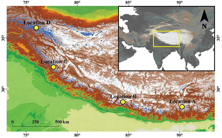
Figure 1. Region of High Mountain Asia, with glaciers outlined in blue and the specific climate regions considered in the study as yellow points. Glacier outlines were obtained from the Randolph Glacier Inventory version 6.0 (2017).

This study has three primary objectives:

1. Quantify the contribution of the albedo-feedback to glacier mass balance.

2. Identify which trigger processes result in a larger albedo-feedback.

3. Determine the climatic characteristics that maximize system gains due to the albedo-feedback.

Methods

Overview

In order to test the magnitude and variability of the albedo-feedback and its trigger processes, this study develops a distributed surface energy and mass balance model with the unique capability to turn individual trigger processes on and off (hereafter referred to as trigger switches). A surface energy and mass balance model is a two-component model that accounts for (1) all major energy fluxes to and from the glacier surface, and (2) the associated mass gains and losses due to snow accumulation and surface melt. Surface energy and mass balance models inherently include feedbacks. The addition of switches in the model allows individual trigger processes to be turned off either individually or in conjunction with other trigger processes. Melt estimates between scenarios in which trigger processes are turned off, both individually and simultaneously, are then compared to one another to evaluate what the net change in melt is as a result of the inherent feedbacks.

The surface energy and mass balance model is first calibrated for one glacier using available climate and mass balance data. After calibration, the same glacier (Figure 2) is evaluated using meteorological data from different climate regions (i.e., the glacier size and shape remain constant, but meteorological inputs are varied). The elevation of the glacier is adjusted for each climate region, simply by adding, or subtracting a fixed value uniformly to the glacier digital elevation model (DEM), such that the annual mass balance is equal to zero. Thus, it approximates steady state for each individual climate setting prior to applying a climate perturbation. The model is run on a daily resolution for 13 years (1 January, 2001 to 31 December, 2013) to ensure high enough temporal resolution to capture important feedback processes and a long enough record to provide representative sampling of climate variability in each target climate region. The exact duration of the model runs is constrained by the available climate data, described below. By utilizing a single glacier morphology, we provide a controlled test of albedo feedbacks for different climate settings without complicating factors such as differing glacier aspect, shading, hypsometry, etc.

FIGURE 2

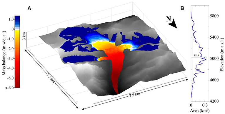
Figure 2. The selected glacier for this study is north facing and is ~16 km². (A) The colors show the extent of the glacier and results of modeled mass balance across the glacier for the control run, with the white areas being the ELA. The spatial resolution is 30 m. (B) Area distribution vs. elevation for the selected glacier, summed over 10 m elevation bands. The ELA is approximated by the black line.

Study Area

HMA is an ideal location to study the effect of the albedo-feedback on glacier mass balance due, in part, to its wide range of precipitation regimes. For example, within HMA, the eastern monsoonal Himalayas receive most of its precipitation during the summer and tend to have high annual precipitation rates; meanwhile, the western Himalayas are more arid, and receive the bulk of their precipitation during the winter (Curio and Scherer, 2016). The diversity of its climates thus makes HMA an excellent location to study the trigger processes that give rise to the albedo-feedback and how they vary spatially and temporally. In addition to its scientific suitability, HMA is also uniquely societally relevant. Meltwater runoff from glaciers feed many of the largest rivers in Asia, which are an important source of water to an estimated 1.4 billion people (Immerzeel et al., 2010). They also play a significant role in global sea level rise, regional water resources, ecosystem stability, energy production, agriculture, and risk management (Barry, 2006; Immerzeel et al., 2010, 2020; Moors et al., 2011; Gardner et al., 2013; Pritchard, 2019; Zemp et al., 2019). While geodetic mass balance estimates have recently shed light on regional patterns of mass balance in HMA (e.g., Gardelle et al., 2013; Brun et al., 2017; Maurer et al., 2019; Shean et al., 2020), the physical processes governing these large-scale patterns remain poorly understood (Azam et al., 2018; Kumar et al., 2019; Maurer et al., 2019). As a result, the projected responses of glaciers in HMA to climate change remain uncertain (Immerzeel et al., 2010; Bolch et al., 2019). By focusing this study on HMA, we will help improve our physical understanding of processes governing the mass balances of these glaciers and their sensitivity to climatic change.

Data

Meteorological inputs needed for the surface energy and mass balance model are from the High Asia Refined analysis (HAR10) (Maussion et al., 2014), a gridded 10 km resolution dataset generated using the Weather Research and Forecast model. HAR10 is available for the period October, 2000 to October, 2014. The primary HAR10 outputs used in this study include daily 2-m air temperature, air pressure, precipitation, relative humidity, incident solar radiation, 10-m wind speed, and incoming longwave radiation, as well as hourly incident solar radiation. The meteorological variables were downscaled to the resolution of a DEM covering the glacier area (downscaling details in section Downscaling). The DEM used in this study is from the ALOS¹ 30 m dataset.

The glacier selected for this study, Chhota Shigri Glacier, is located at 32.23° N 77.51° E (Location C in Figure 1). The glacier was delineated using the Randolph Glacier Inventory v6.0 (RGI Consortium, 2017). The glacier is a clean ice glacier (3.4% debris cover as of 2011; Vincent et al., 2013) and ~16 km². This glacier was chosen in part because there are both geodetic mass balance and in situ data available that overlaps much of the period covered by HAR10, allowing for calibration and validation of the surface energy and mass balance model (Azam et al., 2016, 2019; Brun et al., 2017; Maurer et al., 2019).

Surface Energy and Mass Balance Model

The surface energy budget of a glacier is estimated by:

$\begin{array}{ll}{Q}_m=S_{net}+L_{net}+Q_S+Q_L+Q_P+Q_G& (1)\end{array}$

where Q_m is the net surface energy, S_net is the net shortwave radiative flux, L_net is the net longwave radiative flux, Q_S is the sensible heat flux, Q_L is the latent heat flux, Q_p is the heat flux supplied by precipitation, and Q_G is the subsurface heat flux due to conduction through the snow or ice. Incoming (outgoing) energy fluxes are denoted as positive (negative). Positive (negative) net surface energy is used to warm (cool) the surface up to the melting point (0°C), at which point any remaining positive energy causes the surface to melt. We assume melt run-off in all scenarios here. See Tables S1, S2 for a list of all variables, parameters, and constants used in the model.

Radiative Energy Fluxes

The radiative energy budget consists of all shortwave and longwave radiative fluxes to the surface of the glacier, S_net and L_net, respectively. The net shortwave radiative flux is equal to the difference between the incoming solar radiation and the reflected shortwave radiation, modified by the angle of incidence:

$\begin{array}{ll}{\text{S}}_{\text{net}}={\text{S}}_{\text{in}}(1-\alpha )cos(\theta )& (2)\end{array}$

where S_in is the incoming shortwave radiation, α the surface albedo, and θ the incidence angle. Because the model uses a daily time step, calculation of the incidence angle is not possible with standard methods (which depend on sub daily resolutions). Thus, this model uses a modification which utilizes hourly incoming shortwave radiation from the High Asia Refined analysis:

$\begin{array}{ll}\begin{array}{c}\cos (\theta )={\displaystyle \sum _{\text{h}=1}^{24}{\text{S}}_{{\text{in}}_{\text{h}}}}\cos ({\theta }_{\text{h}})={\displaystyle \sum _{\text{h}=1}^{24}{\text{S}}_{{\text{in}}_{\text{h}}}}\end{array}& (3)\end{array}$

where S_in(h) and θ_h are the incoming shortwave radiation and incidence angle, respectively, at hour h. Here, cos(θ) becomes essentially a scaling factor (between 0 and 1) representing the fraction of solar radiation that reaches the surface of an inclined plane relative to a horizontal plane. The angle of incidence for each hour is calculated as

$\begin{array}{ll}cos({\theta }_{\text{h}})=cos(\beta )cos({\text{Z}}_{\text{h}})+sin(\beta )sin({\text{Z}}_{\text{h}})cos\left({\phi }_{\text{su}{\text{n}}_{\text{h}}}-{\phi }_{\text{slope}}\right)& (4)\end{array}$

where β is the slope angle, Z_h the zenith angle, φ_sun(h) the solar azimuth, and φ_slope the slope azimuth (Garnier and Ohmura, 1968).

Surface albedo, α, on a given day (i) is calculated following Oerlemans and Knap (1998), but uses adjusted values for the parameters (α_frs, α_ice, α_fi, d^*, and t^*) following Mölg and Hardy (2004):

$\begin{array}{ll}{\alpha }^{(\text{i})}=\alpha {}_{\text{s}}^{(\text{i})}+\left({\alpha }_{\text{ice}}-\alpha {}_{\text{s}}^{(\text{i})}\right)exp\left(-\frac{\text{d}}{{\text{d}}^{\text{*}}}\right)& (5)\end{array}$

where α_ice is an albedo for bare ice, d is snow depth (in cm), d^* is an e-folding constant for snow depth, and α_s is the albedo of snow at day (i). α_s is a function of the time since the last snowfall:

$\begin{array}{ll}\alpha {}_{\text{s}}^{(\text{i})}={\alpha }_{\text{fi}}+({\alpha }_{\text{frs}}-\alpha {}_{\text{fi}})exp\left(\frac{\text{s}-\text{i}}{{\text{t}}^{\text{*}}}\right)& (6)\end{array}$

where α_fi is an albedo for firn, α_frs is an albedo for fresh snow, s is the day of the last snowfall event, and t^* is an e-folding time constant that accounts for the decreasing albedo of snow over time. Thus, net shortwave radiation is a function of solar radiation incident at the surface, whether the surface is snow or ice covered, as well as age and depth of the snow.

Net longwave radiative flux (L_net) is equal to the sum of incoming longwave radiation, L_in, and outgoing longwave radiation, L_out:

$\begin{array}{ll}{\text{L}}_{\text{net}}={\text{L}}_{\text{in}}+{\text{L}}_{\text{out}}& (7)\end{array}$

Incoming longwave radiation is calculated in two steps. First, the effective emissivity of the air, ε_a, is calculated from HAR10 temperature, T_a0, and incoming longwave radiation, L₀. This provides a temporally-downscaled, self-consistent estimate of the emissivity of the air.

$\begin{array}{ll}{\epsilon }_{\text{a}}={\text{L}}_0/(\sigma {\text{T}}_{\text{a}0}^4)& (8)\end{array}$

Next, incoming longwave radiation, L_in, is spatially distributed across the glacier using the lapse rate-downscaled air temperature, T_a, such that

$\begin{array}{ll}{\text{L}}_{\text{in}}=\sigma {\epsilon }_{\text{a}}{\text{T}}_{\text{a}}^4& (9)\end{array}$

where σ is the Stefan-Boltzmann constant. Outgoing longwave radiation, L_out, is then given by

$\begin{array}{ll}{\text{L}}_{\text{out}}=-\sigma {\epsilon }_{\text{s}}{\text{T}}_{\text{s}}^4& (10)\end{array}$

where σ is the Stefan-Boltzmann constant, ε_s is the emissivity of the surface, and T_s is the temperature of the surface.

Turbulent Heat Fluxes

The turbulent heat fluxes are calculated following a well-established bulk aerodynamic approach (e.g., Oerlemans, 1992; Wagnon et al., 2003; Mölg and Hardy, 2004; Anderson et al., 2010; Cuffey and Paterson, 2010), whereby the sensible heat flux, Q_s, and the latent heat flux, Q_L, are estimated by:

$\begin{array}{ll}{\text{Q}}_{\text{S}}=\frac{{\rho }_{\text{a}}{\text{P}}_{\text{a}}{\text{c}}_{\text{p}}{\text{k}}_{\text{H}}\text{U}({\text{T}}_{\text{a}}-{\text{T}}_{\text{s}})}{{\text{P}}_0}& (11)\end{array}$

$\begin{array}{ll}{\text{Q}}_{\text{L}}=\frac{0.622{\rho }_{\text{a}}{\text{k}}_{\text{E}}\text{U}{\text{L}}_{\text{v}}({\text{e}}_{\text{a}}-{\text{e}}_{\text{s}})}{{\text{P}}_{\text{a}}}& (12)\end{array}$

where ρ_a is the density of the air at sea level, c_p is the specific heat capacity of the air, U, is the wind speed (at 10 m), T_a, is the temperature of the atmosphere (at 2 m), T_s, is the surface temperature, L_v, is the latent heat of vaporization for water, e_a is the vapor pressure of ambient air (at 2 m), e_s is the vapor pressure of air at the glacier surface, P_a is the air pressure, P₀ is the air pressure at sea level, and k_E and k_H are the bulk transfer coefficients for neutral conditions for latent and sensible heat (respectively), defined (following Webb, 1970) as:

$\begin{array}{ll}{\text{k}}_{\text{H}}=\frac{{\text{k}}_0^2}{ln\left(\frac{{\text{z}}_{\text{m}}}{{\text{z}}_{0\text{m}}}\right)ln\left(\frac{{\text{z}}_{\text{v}}}{{\text{z}}_{0\text{v}}}\right)}& (13)\end{array}$

$\begin{array}{ll}{\text{k}}_{\text{E}}=\frac{{\text{k}}_0^2}{ln\left(\frac{{\text{z}}_{\text{m}}}{{\text{z}}_{0\text{m}}}\right)ln\left(\frac{{\text{z}}_{\text{h}}}{{\text{z}}_{0\text{h}}}\right)}& (14)\end{array}$

where k₀ is the von Karman constant, z_m is the wind speed measurement height above the surface (10 m), z_0m is the roughness length for wind, z_v is the measurement height for water vapor pressure (2 m), z_0v is the roughness length of water vapor, z_h is the measurement height for temperature (2 m), and z_0h is the roughness length of temperature. We adapt constant values (for snow and ice, respectively) for z_0m (0.001, 0.016 m), z_0v (0.001, 0.004 m), and z_0h (0.001, 0.004 m) from Azam et al. (2014).

Precipitation and Conductive Heat Fluxes

The advected heat flux due to liquid precipitation, Q_P, follows the commonly used method (e.g., Singh et al., 2011)

$\begin{array}{ll}{\text{Q}}_{\text{P}}={\text{c}}_{\text{w}}\text{P}({\text{T}}_{\text{a}}-{\text{T}}_{\text{s}})& (15)\end{array}$

where c_w is the specific heat of water, P is the rainfall intensity, T_a is the air temperature, and T_s is the temperature of the surface. This assumes all precipitation falls at air temperature and that precipitation falls as rain if the air temperature is above 2°C.

Conductive heat flux, Q_G, is given by Mölg and Hardy (2004):

$\begin{array}{ll}{\text{Q}}_{\text{G}}=-\frac{{\kappa }_{\text{i}}({\text{T}}_{\text{s}}-{\text{T}}_{\text{z}})}{\Delta {\text{z}}_{\text{i}}}& (16)\end{array}$

where κ_i is the thermal conductivity of ice, Δz_i is the depth in the ice (here Δz_i = 10 m) where the temperature of the ice is assumed to be constant, unaffected by fluctuations in air temperature, and equal to the average annual air temperature at each grid location on the glacier. While snow and ice typically have different thermal conductivities, using a constant thermal conductivity here across the entire glacier surface is unlikely to impact results significantly due to the minimal contribution of Q_G to the overall surface energy budget.

Downscaling

Air temperature and pressure from HAR10 were downscaled from 10 km to 30 m resolution. Temperature downscaling was applied using a constant 6.5°C km⁻¹ lapse rate, the mean tropospheric lapse rate (Hartmann, 1994). While it is well-known that temperature lapse rates vary significantly by region, time of day, season, and even over glacier surfaces (Petersen and Pellicciotti, 2011; Azam et al., 2014; Shea et al., 2015; Thayyen and Dimri, 2018), temperature lapse rate measurements across HMA are not widely available. Additionally, a constant temperature lapse rate provides a consistent means for scaling in different regions of HMA, ensuring that the results for each region are directly comparable.

Air pressure was downscaled using a derivation of the hydrostatic (Equation 17) and the equation of state (Equation 18), as follows.

$\begin{array}{ll}\Delta {\text{P}}_{\text{a}}=-\rho g\Delta h& (17)\end{array}$

$\begin{array}{ll}{\text{P}}_{\text{a}}=\rho {\text{R}}_{\text{d}}{\text{T}}_{\text{v}}& (18)\end{array}$

where ΔP_a is the change in air pressure, ρ is air density, g is the gravity constant, Δh is the change in elevation, P_a is air pressure, R_d is the universal gas constant for dry air, and T_v is the virtual air temperature. T_v is defined as:

$\begin{array}{ll}{\text{T}}_{\text{v}}\equiv \frac{{\text{T}}_{\text{a}}}{1-\frac{\text{e}}{{\text{P}}_{\text{a}}}(1-ϵ)}& (19)\end{array}$

Here, T_a is air temperature, e is vapor pressure, and ϵ is the ratio of gas constants for air and water vapor.

Solving for ρ in Equation (18), substituting equations for ρ and T_v into (Equation 17), and finally, solving for the pressure gradient, ΔP_a/Δh, allows the pressure gradient to be calculated solely as a function of air temperature and pressure:

$\begin{array}{ll}\frac{\Delta {\text{p}}_{\text{a}}}{\Delta \text{h}}=-\frac{{\text{P}}_{\text{a}}\text{g}\left(1-\frac{\text{e}}{{\text{p}}_{\text{a}}}(1-ϵ)\right)}{{\text{R}}_{\text{d}}{\text{T}}_{\text{a}}}& (20)\end{array}$

While it is well-established that precipitation gradients can have significant impacts on glacier mass balances, this study does not apply a precipitation gradient for several reasons. First, precipitation gradients in HMA are known to vary significantly both spatially and temporally but remain poorly constrained (e.g., Singh and Kumar, 1997; Anders et al., 2006; Jarosch et al., 2010; Cuo and Zhang, 2017). Indeed, even neighboring basins can have very different precipitation gradients. Additionally, it is unclear how including a precipitation gradient in this study would improve the robustness of the results found here when glaciers in different climates are likely to have different precipitation gradients. Future studies should evaluate how the precipitation gradient parameterization affects feedback mechanisms. Thus, to maintain direct comparability between regions without adding additional complexities to the model that lack validation, we forego the use of a precipitation gradient in this study.

Surface Temperature Calculation

The surface energy and mass balance model presented here solves for the temperature of the glacier surface and energy available to melt using an iterative method, as follows. Initially, the model assumes that energy available to melt the glacier surface (Q_m in Equation 1) is zero. Using this initial guess for the melt energy, it then calculates the surface temperature. If the calculated surface temperature is ≤0°C, the model records that surface temperature and proceeds to the next time step. However, if the calculated surface temperature is positive, the model sets the temperature of the surface to 0°C and recalculates the energy available to melt. The melt energy is then used to melt the glacier surface.

Model Calibration

The model is calibrated using a combination of in situ measurements available from the World Glacier Monitoring Service (WGMS, 2018) database and geodetic mass balance data (Maurer et al., 2019). In-situ measurements are available in 50–250 m elevation bands along the glacier each year from 2003 to 2006 (Figure 3). The values for the albedo of fresh snow, α_fs (0.85), the albedo of firn, α_fi (0.40), the albedo of bare ice, α_i (0.3), and the phase transition threshold, T_pt (2°C), for partitioning rainfall/snowfall were adjusted until good agreement was reached between the modeled mean annual mass balance profile and the 4 years of in-situ elevation-distributed mass balance measurements.

FIGURE 3

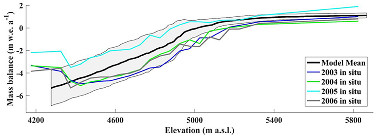
Figure 3. Modeled mean glacier mass balance profile plotted against in-situ glacier mass balance profiles for the years 2003–2006. The shaded area represents one standard deviation from the mean of the modeled mass balance profile from 2001 to 2013.

In addition to comparing the mass balance profiles, the modeled mean annual glacier mass balance (−0.42 m w.e. a⁻¹, for 2001–2013) also compares well with both the geodetic mean annual mass balance (−0.37 m w.e. a⁻¹, for 2000–2016; Maurer et al., 2019) and in situ mean annual mass balance (−0.59 m w.e. a⁻¹, for 2002–2012; Azam et al., 2016). Additional mass balance estimates for Chhota Shigri Glacier covering a range of time periods are summarized by Azam et al. (2019).

Model Sensitivity

Here we test the sensitivity of modeled glacier mass balance to key input parameters to determine which parameters are most likely to affect the results presented here (Figure 4). The test was performed using inputs for Region C, the default location of Chhota Shigri Glacier. Ten parameters were varied independently in the model with both an increased and a decreased value relative to the default values used in this study. The results indicate that the model is most sensitive to the precipitation phase threshold, followed by the albedo of ice, the e-folding time constant for determining the evolution of albedo for aging snow, and the temperature lapse rate. This suggests that the model is most sensitive to parameters that have direct influences on surface albedo.

FIGURE 4

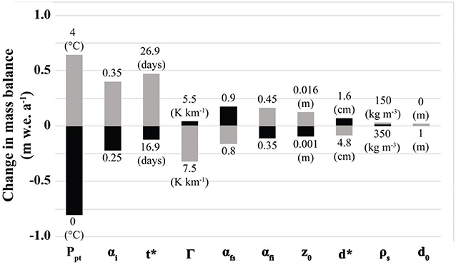
Figure 4. Results from testing glacier mass balance sensitivity to input parameter values. Gray bars represent increased parameter values (relative to the defaults), while black bars represent decreased parameter values. The range of parameter values tested is included above and below each bar. See Table S1 for default parameter values.

Feedbacks and Triggers

Here we present a description of the individual trigger processes targeted in this study (see Figure 5 for a schematic diagram of each), as well as an explanation of how the model “turns off” each trigger process (i.e., the switches). Note that all three trigger processes described initiate the albedo-feedback, but that each impacts albedo via a different mechanism. We name each trigger process (e.g., “accumulation trigger”) only to distinguish between the mechanism that leads to a change in the albedo of the surface. In reality, because albedo and surface melt are dependent on one another, any mechanism that affects albedo will likely result in a feedback loop. Note also that all three trigger processes are a result of changes in precipitation phase but are measured by their net effect on glacier melt.

FIGURE 5

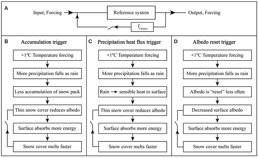
Figure 5. Schematic diagram of feedbacks and trigger processes. (A) Illustrates feedbacks generally. (B–D) Illustrate the individual trigger processes tested in this study. Top panel adapted from Roe (2009).

Trigger Process Descriptions

Accumulation trigger

An increase in air temperature increases the fraction of precipitation that falls as rain. This results in less snowfall, which leads to a thinner snow cover. Thinning the snow cover decreases the albedo of the surface, which causes the surface to absorb more energy and triggers a positive feedback loop. This further thins the snow cover, etc.

Precipitation heat flux trigger

An increase in air temperature increases the fraction of precipitation that falls as rain. This results in an increase in the heat flux supplied by precipitation to the surface, which causes increased melt. Increased melt leads to a thinner snow cover, which decreases the albedo of the surface and triggers a positive feedback loop. This causes the surface to absorb more energy, which further increases melt, etc.

Albedo reset trigger

An increase in air temperature increases the fraction of precipitation that falls as rain. This results in fewer snowfall events on the glacier, which “resets” the albedo of the surface less frequently (i.e., because each snowfall event “resets” the surface albedo to that of fresh snow). Resetting the albedo of the surface less frequently decreases the albedo of the surface, which causes the surface to absorb more energy. This causes increased melting resulting in a thinner snow cover, which further decreases the albedo of the surface, etc.

Trigger Process Switches and Albedo Feedback

To facilitate conceptualization of the functionality of the trigger switches used in this study, we present an idealized scenario with which we will present each trigger switch. In each case, measuring the strength of the albedo-feedback necessarily requires three distinct iterations of the scenario. First, the surface energy balance model is run with present-day climate as the input (ΔT = 0°C, and all trigger switches remain on). Note that when all trigger process switches are turned on, the full magnitude of the albedo-feedback is included in the calculation. This is the control run. Second, the model is run using a +1°C temperature change (ΔT = +1°C, and all trigger switches remain on). Third, the model is run using a +1°C temperature change (ΔT = +1°C), but with the trigger switch(es) turned off. Note that if all trigger switches are turned off, the albedo-feedback mechanism is turned completely off and no albedo-feedbacks occur. If a subset of trigger switches are turned off, only a portion of the albedo-feedback mechanism operates. The following idealized scenario will describe the first two iterations of the scenario, while each feedback description thereafter will describe the third iteration of the scenario, with the respective trigger switch turned off.

Consider an idealized scenario where the average temperature at location x at time i on the glacier is 1.5°C. It snows (because precipitation is assumed to fall at air temperature and in a solid state if the temperature is <2°C). This is the control run. In the second iteration, a +1°C change is applied (ΔT = +1°C), increasing the temperature to 2.5°C. In this iteration, it now rains instead of snows. Because it rains rather than snows, (1) the snowpack is thinner (Δd is negative relative to the control; Equation 5), (2) rain now supplies heat to the surface (ΔQ_P is positive relative to the control; Equation 15), potentially further decreasing snowpack thickness, and (3) surface albedo is not reset (s stays the same, rather than being set equal to i as in the control; Equation 6). All three of these trigger processes decrease surface albedo and initiate the albedo-feedback loop.

Trigger switches turn off the trigger processes to determine the change in melt due to a temperature change in the absence of that process. The following descriptions of the trigger switches are described in the context of the scenario presented above.

Accumulation switch

Turning the accumulation trigger off (with ΔT = +1°C) would force the thickness of the snowpack to remain the same as if there had been no temperature change (Δd = 0), but would not affect the impact of ΔT on the precipitation heat flux (ΔQ_P is positive) or albedo reset (s stays the same, rather than being set equal to i) due to changes from snow to rain. Thus, we artificially keep the snowpack thickness the same as in the control run but allow the precipitation heat flux and albedo reset triggers to respond to the temperature change and associated change in precipitation phase from snow to rain. In this scenario, we are testing the magnitude of the albedo-feedback when changes in snowpack thickness due to changes in temperature are not included.

Precipitation heat flux switch

Turning the precipitation heat flux trigger off (with ΔT = +1°C) would prevent the precipitation (which would now fall as rain) from supplying any additional heat to the surface (ΔQ_P = 0). In this scenario, the snowpack is thinner relative to the control (Δd is negative) and the surface albedo is not reset (s stays the same, rather than being set equal to i). In other words, we artificially keep the heat flux supplied by precipitation the same as in the control run, but allow the accumulation and albedo reset triggers to respond to the temperature change. In this scenario, we are testing the magnitude of the albedo-feedback when changes in precipitation phase due to changes in temperature are not included.

Albedo reset switch

Turning the albedo reset trigger off (with ΔT = +1°C) would cause the surface albedo to reset (s is set equal to i), even though precipitation would actually fall as rain at 2.5°C. In this scenario, the snowpack is thinner relative to the control (Δd is negative) and the heat flux from precipitation is still supplied to the surface (ΔQ_P is positive). In other words, turning off the albedo reset trigger forces the albedo to reset with the same frequency as in the control run, but allows the accumulation and precipitation heat flux triggers to respond to the temperature change. In this scenario, we are testing the magnitude of the albedo-feedback when changes in the frequency of snowfall events due to changes in temperature are not included.

Gains Due to Feedbacks

We use system gains as a measure of how strongly the albedo-feedback and trigger processes impact glacier mass balance in a given region. The system gain due to feedbacks, G, is “the factor by which the system response has gained due to the inclusion of the feedback(s), compared with the reference-system response” (Roe, 2009), here defined as:

$\begin{array}{ll}G=\frac{\Delta \text{m}}{\Delta {\text{m}}_{\text{Ref}}}=\frac{({\text{m}}_{\text{T}1}-{\text{m}}_{\text{T}0})}{({\text{m}}_{\text{T}1\text{F}}-{\text{m}}_{\text{T}0})}& (21)\end{array}$

where Δm is the change in melt (including full albedo feedback with all trigger processes turned on) resulting from a perturbation to the system (i.e., a change in albedo resulting from a +1°C temperature change), Δm_Ref is the change in melt (with only a subset of trigger processes turned on) resulting from a +1°C temperature change, m_T0 is glacier melt with no temperature change, m_T1 is glacier melt with a +1°C temperature change and all trigger processes turned on, and m_T1F is glacier melt with a +1°C temperature change with the trigger process(es) turned off.

Regions

Four regions with significantly different annual climatologies were selected from within the HAR10 dataset (Figure 6 and Table 1). Each “region” in this context refers only to the use of a single 10-km grid location from the HAR10 dataset. The meteorological data for each region in this study is therefore treated effectively like data collected at a single weather station. The meteorological data from these regions were used as input to the model to test the dependence of the albedo-feedback on precipitation amount and timing. For each control scenario, the glacier elevation is adjusted to force each glacier into equilibrium (i.e., so the magnitude of melt is equal to the magnitude of accumulation for the 13-year model run). Note that for the control run in Region C, the actual location of Chhota Shigri Glacier, the elevation is also adjusted to force it into equilibrium. It maintained its original elevation only when it was being calibrated and validated. This forced equilibrium in all regions is done in order to make results more directly comparable between all four regions.

FIGURE 6

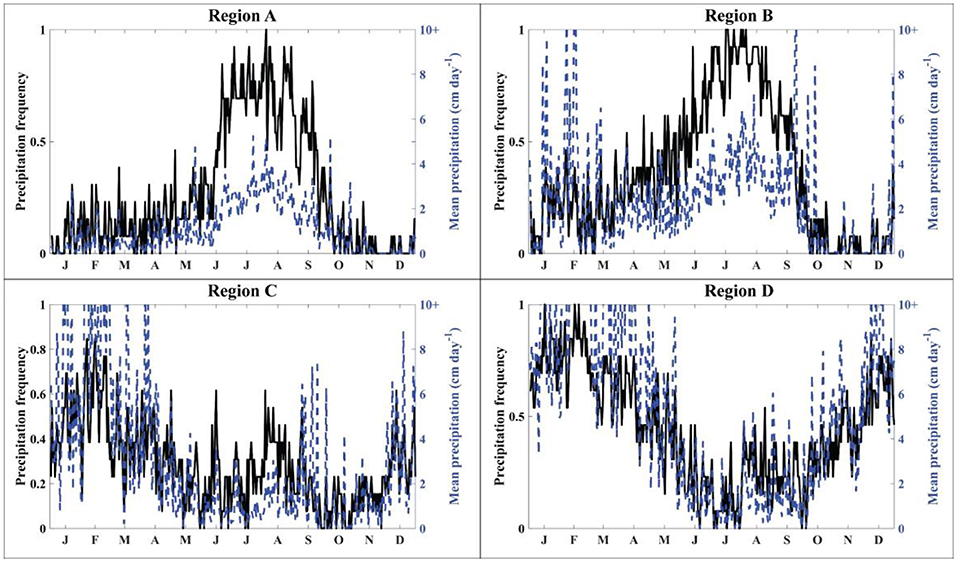
Figure 6. Precipitation frequency (black line) and mean precipitation (blue dashed line) averaged for each day (e.g., each 1 March is averaged) across 2001–2013 for each region. Precipitation frequency as presented here is the number of times a given day exhibited precipitation divided by the total number of years of data (13). For example, if it rained all 13 years on 1 June, then the precipitation frequency for that day would be 1.

TABLE 1

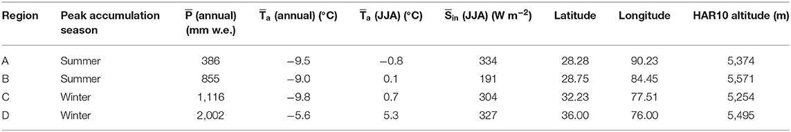
Table 1. Summary of climate conditions for each region.

Results

Energy Budgets

The energy budget for each region provides a diagnostic tool for examining the processes that lead to differences in glacier mass balance and system gains between regions. Figure 7 shows the energy budgets for each climate region for the control run, averaged over the glacier surface and for each day. Energy fluxes in each region are within reasonable ranges, as compared to other studies in HMA (e.g., Kayastha et al., 1999; Fujita and Ageta, 2000; Zhang et al., 2013; Azam et al., 2014; Acharya and Kayastha, 2018). Note that the turbulent heat fluxes are generally much smaller than the radiative fluxes for all climate regimes (Figure 7). In addition, the variability and magnitude of the fluxes vary between regions (Table 2). For example, incident shortwave is strongly influenced by clouds, with the largest impact occurring in Region B, where precipitation is also largest during those summer months.

FIGURE 7

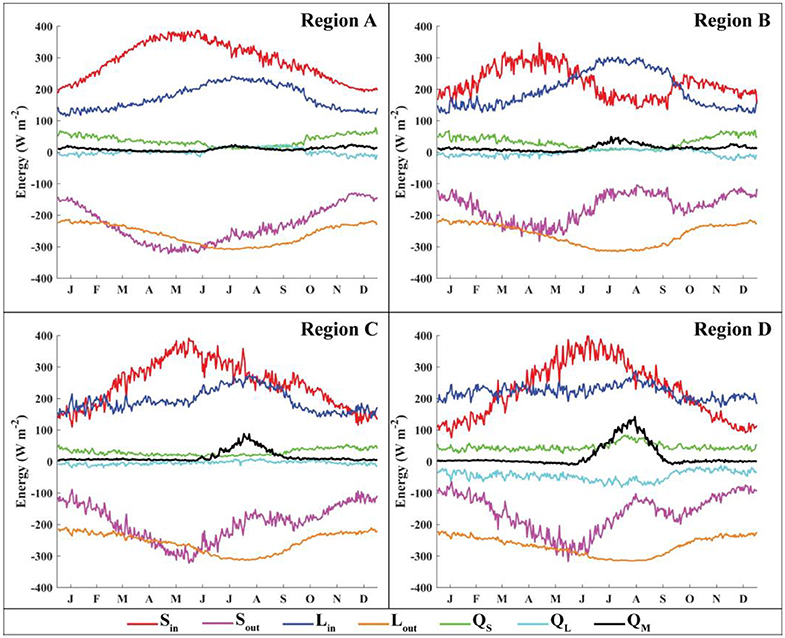
Figure 7. Energy fluxes for the control run averaged over the entire glacier for each day over the 13 years covered by this study. Note that Q_G, the heat conducted into the glacier, is not shown here due to its minimal contribution to the overall energy budget.

TABLE 2

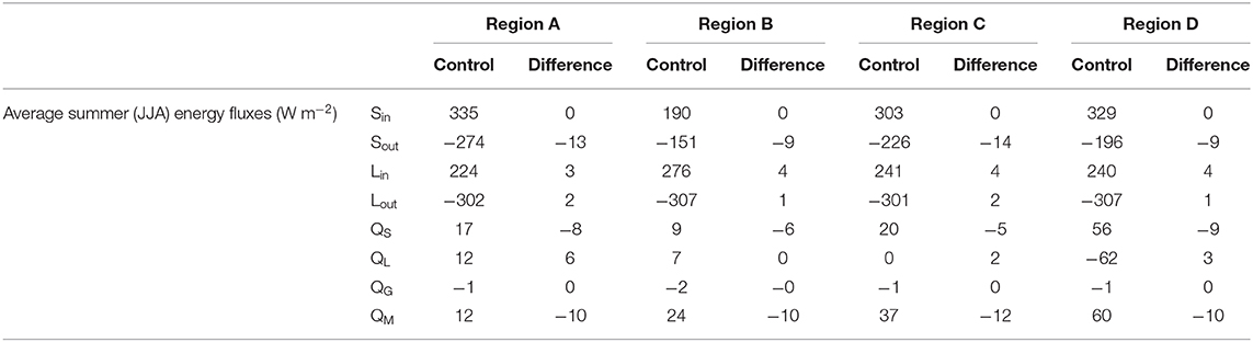
Table 2. Summary of energy fluxes (Figure 7) and changes in energy fluxes due to a +1°C temperature change (Figure 8).

The change in energy budgets for each region due to a temperature change is shown in Figure 8. As expected, a +1°C temperature change results in an increase in the net surface energy budget in each region. Regions A, B, and C exhibit a peak increase in net shortwave radiation near the middle of the melt season. This occurs because the average summer temperature in these regions is close to 0°C, where a temperature change can shift the precipitation phase from snow to rain for a large area of the glacier, thereby decreasing the albedo. Figure 9 shows the change in precipitation phase for the temperature change and that the maximum change in precipitation phase occurs near the middle of the melt season for regions A, B, and C. In comparison with regions where the increase in net shortwave radiation peaks near the middle of the melt season, Region D exhibits increased net shortwave radiation that is maximized near the beginning and end of the melt season. This corresponds to an increased fraction of precipitation falling as rain at these times (Figure 9), which decreases the albedo and increases the absorbed shortwave radiation. During the middle of the melt season, however, precipitation falls infrequently enough during the summer that it has little effect on albedo (Region D). The comparison in energy budgets and energy changes between regions suggests the variations and changes in melt and system gains will depend on the initial climate setting.

FIGURE 8

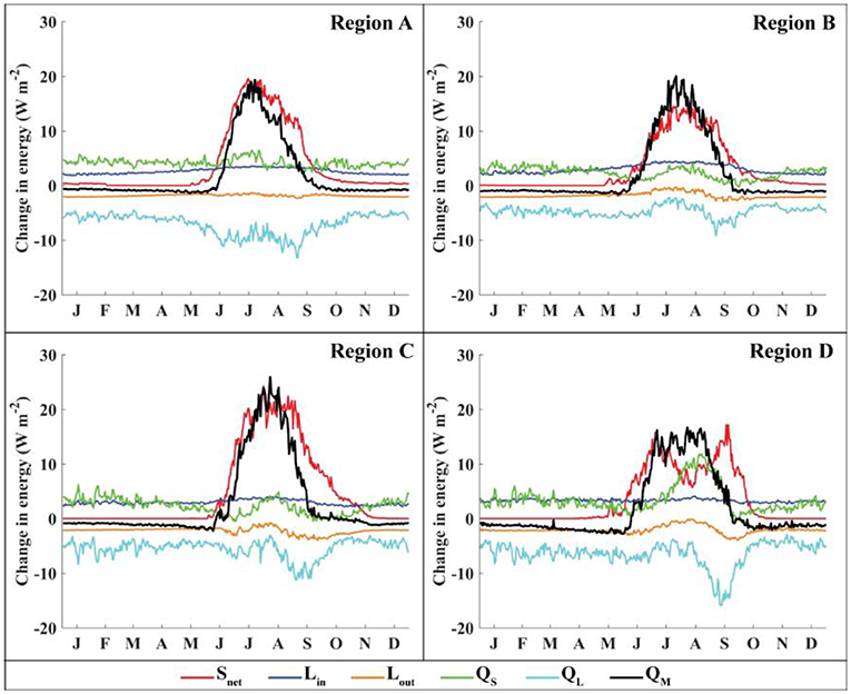
Figure 8. Change in energy fluxes, for a 1°C temperature increase, averaged over the entire glacier and for each day over the 13 years covered by this study.

FIGURE 9

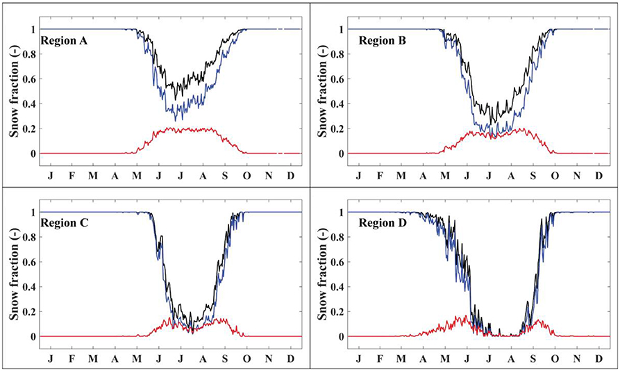
Figure 9. Fraction of snow precipitation to total precipitation averaged for each day (for all 13 years of the model runs) over the entire glacier surface for the control run (black lines) and for +1°C temperature change (blue lines). Discontinuities in some lines indicate days in which no precipitation occurred on that day for all 13 years. The red lines show the difference in fraction of precipitation that falls as snow between the control runs (ΔT = 0°C) and runs with a temperature change (ΔT = +1°C).

Mass Balance

Local mass balance for all regions under both summer- and winter-dominated precipitation regimes are shown in Figure 10. Importantly, melt and accumulation gradients fall within reasonable ranges. As expected, an increase in temperature decreases the mass balance of the glacier within all four climate settings, but the amount of change is not uniform. In particular, the mean mass balance changes are largest in Region B (−0.60 m w.e. a⁻¹) where incident shortwave radiation is lowest during the melt season, and smallest in Region D (−0.47 m w.e. a⁻¹) where average summer temperature is significantly higher than in any other region. Thus, while the change in temperature is the same for all scenarios, the mass balance response is dependent upon the climate setting at the time of the change.

FIGURE 10

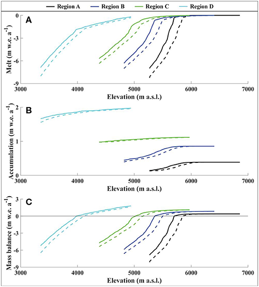
Figure 10. Summary of glacier melt (A), accumulation (B), and mass balance (C) for each region with no temperature change (solid lines) and with a +1°C temperature change (dashed lines). Values are averaged over 10 m elevation bands across the glacier surfaces.

System Gain

The system gain, as used in this study, is a measure of how strongly the albedo-feedback impacts glacier melt in a given region for the given trigger process(es) (Equation 21). The gain should not be interpreted as the increase in melt expected from a +1°C temperature change, but rather as the gain due to modeling melt with and without feedbacks included. For example, the gain for Region A with all trigger switches turned off is equal to 6 (Figure 11). This does not mean that the melt is 6 times greater with a temperature increase of +1°C as compared to the control run. Indeed, the average melt increases by <10% in Region A (Figure 10). A gain of 6 means that the additional melt that resulted from a +1°C temperature increase would be 6 times less had the albedo-feedback not been included. In other words, five sixths (~80%) of the melt increase due to the temperature change is attributable to the albedo-feedback.

FIGURE 11

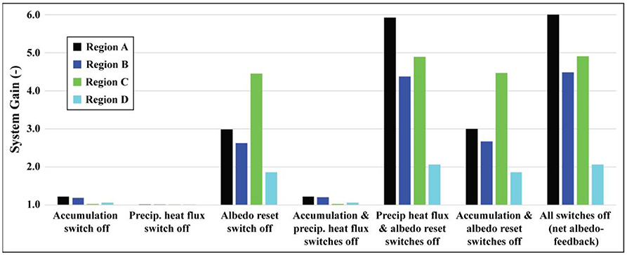
Figure 11. System gains (averaged across the glacier surface) associated with turning each trigger switch off. Gains correspond to the fractional increase in melt due to the inclusion of the trigger process(es).

The system gains are highly variable for the four different climate settings (Figure 11), with higher system gains indicating conditions under which glaciers have larger responses to a trigger process (e.g., increasing fraction of precipitation falling as rain) than in regions with lower system gains. Here we find that system gains due to the albedo-feedback loop (all trigger switches off) are highest in Region A, where incident shortwave radiation (Figure 7) is high during the summer and where frequent summer snowfall events (Figure 6) have a large impact on melt season albedo. In Region B, frequent summer snowfall events are even more frequent than in Region A, but incident shortwave radiation during the summer is low, thereby muting the effects of these feedbacks. In contrast, Region C has relatively few summer snowfall events, but significantly higher incident shortwave radiation, resulting in somewhat higher overall system gains than Region B. This highlights the importance of both summer snowfall frequency and availability of shortwave radiation in controlling feedback strength. Finally, Region D exhibits the lowest overall gains, despite its high incident shortwave radiation, because precipitation events are infrequent during the summer and typically fall as rain.

Spatially on the glacier, the system gain is maximized between the equilibrium line altitudes (ELAs) with a 0 and +1°C change (Figure 12; see also Figure S1 for distributed maps of system gains for the four regions). This region on the glacier can exhibit a localized (elevation-averaged) system gain of up to 60. This localized maximum is due to a larger change in snowfall frequency near the ELA due to a +1°C change in comparison with other locations on the glacier.

FIGURE 12

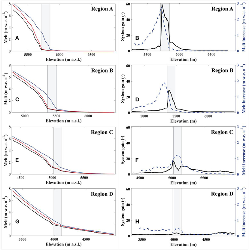
Figure 12. Glacier melt and system gains averaged over 10 m elevation bands across the glacier surface. Panels (A,C,E,G) show average melt with ΔT = 0°C (black line), ΔT = +1°C with all trigger switches turned on (blue line), and ΔT = +1°C with all three trigger switches turned off (red line). Panels (B,D,F,H) show system gains (black line) and average melt increase (dashed blue line) for ΔT = +1°C (with all trigger switches turned on) relative to the control run. The gray rectangle in each plot shows the shift in ELAs due to a temperature forcing of +1°C (i.e., the left side of the rectangle is the ELA with ΔT = 0°C, while the right side of the rectangle is the ELA with ΔT = +1°C).

Of the three trigger processes tested, the albedo reset trigger is consistently the strongest, producing a gain of up to 4.5 (Region C) on its own. This is consistent with findings by Azam et al. (2014) in which they found that the intensity of summer snowfall events was one of the strongest drivers of annual mass balance on Chhota Shigri Glacier due to its strong influence on surface albedo. The precipitation heat flux trigger proved to be negligible in all scenarios. The accumulation trigger produced a maximum gain of 1.2 (Region A). Accounting for all three trigger processes together, the total gains due to the albedo-feedback ranged from 2.1 (Region D) to 6.0 (Region A).

Discussion

Implications/Relevance

In this study, a single glacier was artificially shifted between multiple climate regimes using somewhat idealized scenarios. These results represent a systematic quantification of the contribution of the albedo-feedback to glacier mass balance. Actual feedback contributions on glaciers throughout HMA are likely highly spatially and temporally heterogeneous. However, these results highlight the potential importance of feedbacks on glacier mass balance and its modeling, as well as the conditions under which the albedo-feedback is most important to glacier mass balance. They also provide a first-order estimate of the magnitude of the albedo-feedback contribution, as well as the trigger processes that initiate it, for four very different climate settings.

Most importantly, these results demonstrate that the potential impact of the albedo-feedback on glacier mass balance can be significant. Furthermore, the impact of this feedback is maximized when (1) the accumulation season and the ablation season are synchronous (i.e., summertime accumulation), (2) the frequency of snowfall events is high during the ablation season, and (3) the incoming solar radiation is high during the ablation season. This highlights the importance of the timing, frequency, and form of precipitation events in relation to the ablation season. It may also help explain findings suggesting that melt-dominated regions are often significantly more sensitive to changes in summer temperature than precipitation amount, such as in the monsoonal Himalayas (e.g., Kayastha et al., 1999; Fujita, 2008; Azam et al., 2014; Liang et al., 2018).

Because of the complex ways in which feedbacks interact with one another, even feedbacks that contribute minimally on their own can have significant impacts when other feedbacks are present. In other words, feedbacks are not simply additive (Roe, 2009). This is also true for the individual trigger processes considered here. For example, in Region A, turning triggers 1 and 3 off independently produces a system gain of 1.2 and 3.0, respectively. However, turning triggers 1 and 3 off together produces a system gain of 6.0, which is a 1.8 larger gain than if they were simply additive. Despite this, the contribution of the precipitation heat flux trigger to the overall albedo-feedback is essentially negligible, even in combination with the other two trigger processes tested. This is because the amount of heat supplied by precipitation is so small in comparison with all other energy fluxes that the increased temperature change negligibly changes the amount of energy supplied by precipitation. Thus, trigger processes due to snowpack thickness and the frequency of snowfall events during the ablation season compound each other, while heat supplied by precipitation has little direct effect.

Of the three trigger processes tested, the most significant in terms of glacier mass balance is the albedo reset trigger. This highlights the need to improve both albedo and shortwave radiation parameterizations in future energy balance models, as small inaccuracies in either can be amplified significantly by the albedo-feedback.

While system gains vary both spatially and temporally, they are usually the highest near the ELA. This is likely because the ELA has a maximizing balance. Locations where bare ice is exposed for much of the season (i.e., the glacier toe) are often warm enough that summer precipitation events predominantly occur as rain rather than snow. Meanwhile, locations well above the ELA are cold enough that a small increase in temperature does not change the frequency of snowfall events by a significant amount. The ELA, however, is both cold enough that it can snow relatively frequently, but warm enough that a small change in temperature can have a significant effect on the fraction of precipitation that falls as snow. Because of this effect, overall glacier response to the albedo-feedback probably depends strongly on glacier hypsometry. For example, the albedo-feedback is likely to be more significant on glaciers with large proportions of their area at elevations near the ELA. The Chhota Shigri Glacier does have a large proportion of its area near the ELA (Figure 2), and therefore the magnitude of the albedo-feedback modeled here are likely to be maximized. While outside the scope of this paper, this potential dependency between glacier-wide feedback magnitude and glacier hypsometry should be evaluated in future studies.

Because the total system gain from the albedo-feedback is highly dependent on incident solar radiation, effects of valley wall shading and cast shadowing likely dampen the effects of the albedo-feedback, especially on north-facing glaciers and glaciers in especially steep topography. Though these processes can be very important for glacier mass balance, their effects are frequently neglected or oversimplified in models because of the difficulties involved in modeling them (Olson and Rupper, 2019). Additionally, future studies should examine temporal patterns in feedbacks on diurnal timescales. This study necessarily neglected this aspect due to its daily time step.

Regional Significance

This study uses a theoretical framework to evaluate the relative importance of the albedo-feedback in different climate settings. For discussion purposes, we extend the results of the theoretical approach to the full region of HMA. An examination of the physical drivers of this feedback throughout the region provides a rough estimate of the spatial variability in feedbacks across HMA. For this, we examine the sum of the z-scores (Figure 13, bottom panel) of average summer precipitation frequency (Figure 13, top panel) and average summer incoming solar radiation (Figure 13, middle panel). These two variables are chosen in this analysis since the results in this study show that these are the variables that largely drive the magnitude of the albedo-feedback. Z-scores, z_s, for average summer precipitation frequency (calculated identically for average summer incoming solar radiation) are calculated as:

$\begin{array}{ll}{z}_s=\frac{(x-\mu )}{s_{dev}}& (22)\end{array}$

where x is the average summer (JJA) precipitation frequency (incoming solar radiation) at a given point in HMA, μ is the average summer (JJA) precipitation frequency (incoming solar radiation) for all glaciated regions covered by HAR10, and s_dev is the standard deviation of the average summer precipitation frequency (incoming solar radiation). This analysis is performed using raw data from HAR10, and thus utilizes a 10 km grid spacing. Only grid squares in HAR10 that contain glaciers (as defined by the RGI glacier masks) are considered in this analysis.

FIGURE 13

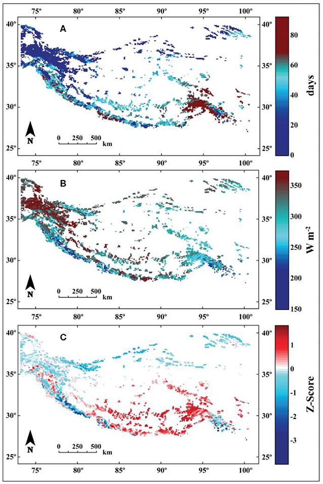
Figure 13. (A) Mean summer (JJA) precipitation frequency. (B) Mean summer incoming shortwave radiation. (C) The sum of the z-scores for the top and middle panels. Assuming these two factors (top two panels) are approximately equally weighted in their contribution to feedbacks, this should provide a rough approximation of where glaciers are likely to be more sensitive to feedbacks (where a higher z-score total corresponds to higher feedback potential). Meteorological data used in this analysis was obtained from HAR10.

In general, this simple exercise suggests that the magnitude of the albedo-feedback should maximize (i.e., highest total Z-score) in HMA in the central to eastern Himalayas and interior Tibetan Plateau, assuming HAR10 captures the regional variability in summer precipitation frequency and solar radiation reasonably well (Table S3). These regions correspond to regions where the summer monsoon plays a large role in regional climate and where solar radiation is relatively high. In these locations, glacier albedo is likely to be highly sensitive to recent weather events, and thus highly variable. This high variability in summertime albedo is likely to give rise to a stronger feedback, particularly in locations where incoming solar radiation is also high.

The regions with the lowest estimates for the albedo-feedback (lowest total Z-score) are the western Himalayas and Kunlun Shan, where the summers are especially dry. Because these locations receive little precipitation during the summer, glacier albedo is likely less variable than in summer accumulation regions. Even in regions with high incoming solar radiation during the summer, changes in air temperature are unlikely to have a significant impact on summertime albedo. Thus, they are likely less sensitive to the albedo-feedback than in summer accumulation regions.

While this simple analysis likely does not perfectly capture the spatial patterns of the albedo-feedback strength in HMA, it highlights the idea that feedbacks across HMA are likely to be highly spatially and temporally variable. However, this analysis is greatly oversimplified. For example, it does not consider temperature, which is likely to have significant impacts on snowline elevation and precipitation phase. It also does not consider heterogeneous warming across the region or glacier hypsometries, which will also have a significant effect on albedo-feedback strength. Despite this, it provides a rough estimate of what parts of HMA have high potential for maximizing the albedo-feedback due to the climatic setting.

Assumptions and Simplifications

The results and discussion presented above must necessarily be interpreted within the context of the theoretical framework of the study. As such, the following discussion examines the capabilities and limitations of the model and its findings.

This study focused only on the spatial distribution of the albedo-feedback and three of its trigger processes, but neglected feedbacks stemming from other glacier surface processes. Additional opportunities exist to examine the effects of feedbacks associated with valley wall shading, aspect, rain-on-snow, and melt/refreeze, among others, as well as other trigger processes that could also initiate the albedo-feedback. While these were outside the focus of this study, future studies should examine the interactions and contributions of such feedbacks.

Estimating precipitation over a glacier is inherently difficult, particularly in regions with complex topography and minimal in situ measurements (e.g., Maussion et al., 2014). Indeed, precipitation estimates from reanalysis products have been shown to have large discrepancies compared to in situ data (Sun et al., 2018). Despite this, the purpose of this study is not to accurately estimate the mass balance of glaciers across the region. Rather, the study aims to isolate the physical drivers of the albedo-feedback on glacier surfaces and provide a first order estimate of the strength of the trigger processes that initiate it. To this end, we do not expect to accurately model precipitation in each region. The larger aim is to create feasible climate scenarios that glaciers in different climate regimes could be reasonably expected to exist in, and to provide a direct comparison between these climate regimes. In this study, we chose not to include a precipitation gradient in order to make the idealized scenarios as directly comparable as possible in lieu of the limited constraints on precipitation gradients on glaciers in HMA. This oversimplification likely affects the precise feedback patterns across the glacier, but it is unlikely to change the relative importance of the trigger processes identified in this study.

Conclusions

This study develops a surface energy and mass balance model to quantify the contribution of the albedo-feedback to glacier mass balances in different climatic regions of HMA. It further quantifies the individual contributions of three unique trigger processes (accumulation amount, frequency of snowfall events, and precipitation heat flux) to the overall magnitude of the albedo-feedback. The model includes “trigger switches” that can be toggled on and off to evaluate individual and combined effects from trigger processes on the albedo-feedback, and how they contribute to glacier mass balance. The model applies meteorological data from the High Asia Refined analysis to a single glacier, and artificially moves this glacier into four different climate settings.

The results show that up to 80% of the glacier-averaged melt increase from a +1°C temperature change can be attributed to the albedo-feedback. The strength of this feedback is most strongly dependent on the timing and frequency of snowfall events, and on the magnitude of shortwave radiation during the melt season. Specifically, system gains are maximized when the maximum frequency of snowfall events occurs concurrently with the melt season in a region where incoming shortwave radiation is high. Furthermore, system gains in each region are typically maximized near the ELA.

Exact magnitudes of system gains vary significantly for different trigger processes. The precipitation heat flux trigger tested here is found to be essentially negligible, even in the presence of other trigger processes that might serve to amplify its effects. The albedo reset trigger is consistently the strongest of the trigger processes tested here. Overall this study suggests that physical processes that affect albedo (e.g., melt, snow metamorphism, rain-on-snow, etc.) can have a significant effect on the net system gain of the albedo-feedback, and therefore on glacier mass balance. As a result, glacier modeling studies examining regions whose glacier mass balances are dominated by melt will benefit from improved parameterizations or process models for processes such as the temporal evolution of albedo, precipitation phase, and direct/diffuse shortwave radiation.

Data Availability Statement

Publicly available datasets were analyzed in this study. This data can be found here: https://www.klima.tu-berlin.de/index.php?show=forschung_asien_tibet_har&lan=en.

Author Contributions

EJ developed the model described in the paper, performed the analyses, and created all figures. SR advised and oversaw the project, wrote some sections of the paper, and edited all of the content.

Funding

We acknowledge funding to SR for support of this research (NSF EAR 1600587 and NASA HMA NNX16AQ61G).

Conflict of Interest

The authors declare that the research was conducted in the absence of any commercial or financial relationships that could be construed as a potential conflict of interest.

Acknowledgments

We would also like to thank Simon Brewer and Rick Forster for their invaluable feedback on the research and on early manuscript drafts.

Supplementary Material

The Supplementary Material for this article can be found online at: https://www.frontiersin.org/articles/10.3389/feart.2020.00129/full#supplementary-material

Footnotes

1. ^Global Digital Surface Model “ALOS World 3D - 30m” (AW3D30). Available online at: http://www.eorc.jaxa.jp/ALOS/en/aw3d30/ (accessed May 5, 2017).

References

Acharya, A., and Kayastha, R. (2018). Mass and energy balance estimation of Yala Glacier (2011-2017), Langtang Valley, Nepal. Water 11:6. doi: 10.3390/w11010006

CrossRef Full Text | Google Scholar

Anders, A., Roe, G. H., Hallet, B., Montgomery, D. R., Finnegan, N., Putkonen, J., et al. (2006). Spatial patterns of precipitation and topography in the Himalaya. Geol. Soc. Am Special Pap. 398, 39–53. doi: 10.1130/2006.2398(03)

CrossRef Full Text | Google Scholar

Anderson, A., Mackintosh, A., Stumm, D., George, L., Kerr, T., Winter-Billington, A., et al. (2010). Climate sensitivity of a high-precipitation glacier in New Zealand. J. Glaciol. 56, 114–128. doi: 10.3189/002214310791190929

CrossRef Full Text | Google Scholar

Arnold, N. S., Rees, W. G., Hodson, A. J., and Kohler, J. (2006). Topographic controls on the surface energy balance of a high Arctic valley glacier. J. Geophys. Res. Earth Surf. 111:F02011. doi: 10.1029/2005JF000426

CrossRef Full Text | Google Scholar

Azam, M., Wagnon, P., Berthier, E., Vincent, E., Fujita, K., and Kargel, J. (2018). Review of the status and mass changes of Himalayan-Karakoram glaciers. J. Glaciol. 64. 61–74. doi: 10.1017/jog.2017.86

CrossRef Full Text | Google Scholar

Azam, M. F., Ramanathan, A. L., Wagnon, P., Vincent, C., Linda, A., Bahadur Singh, V., et al. (2016). Meteorological conditions, seasonal and annual mass balances of Chhota Shigri Glacier, western Himalaya, India. Ann. Glaciol. 57, 328–338. doi: 10.3189/2016AoG71A570

CrossRef Full Text | Google Scholar

Azam, M. F., Wagnon, P., Vincent, C., Al, R., Kumar, N., Srivastava, S., et al. (2019). Snow and ice melt contributions in a highly glacierized catchment of Chhota Shigri Glacier (India) over the last five decades. J. Hydrol. 574, 760–773. doi: 10.1016/j.jhydrol.2019.04.075

CrossRef Full Text | Google Scholar

Azam, M. F., Wagnon, P., Vincent, C., Ramanathan, A. L., Favier, V., Ramanathan, A. L., et al. (2014). Processes governing the mass balance of Chhota Shigri Glacier (Western Himalaya, India) assessed by point-scale surface energy balance measurements. Cryosphere 8, 2195–2217. doi: 10.5194/tc-8-2195-2014

CrossRef Full Text | Google Scholar

Barry, R. G. (2006). The status of research on glaciers and global glacier recession: a review. Prog. Phys. Geogr. 30, 285–306. doi: 10.1191/0309133306pp478ra

CrossRef Full Text | Google Scholar

Bolch, T., Shea, J., Liu, S., Azam, M., Gao, Y., Gruber, S., et al. (2019). “Status and change of the cryosphere in the extended Hindu Kush Himalaya Region,” in Mountains, Climate Change, Sustainability and People, eds P. Wester, A. M. A. Mukherji, and A. B. Shrestha (Cham: Springer), 229–232. doi: 10.1007/978-3-319-92288-1_7

CrossRef Full Text | Google Scholar

Brun, F., Berthier, E., Wagnon, P., Kääb, A., and Treichler, D. (2017). A spatially resolved estimate of High Mountain Asia glacier mass balances from 2000 to 2016. Nat. Geosci. 10, 668–673. doi: 10.1038/ngeo2999

PubMed Abstract | CrossRef Full Text | Google Scholar

Cuffey, K. M., and Paterson, W. S. B. (2010). The Physics of Glaciers, 4th edn. Burlington, MA: Butterworth-Heinemann.

Google Scholar

Cuo, L., and Zhang, Y. (2017). Spatial patterns of wet season precipitation vertical gradients on the Tibetan Plateau and the surroundings. Sci. Rep. 7:5057. doi: 10.1038/s41598-017-05345-6

PubMed Abstract | CrossRef Full Text | Google Scholar

Curio, J., and Scherer, D. (2016). Seasonality and spatial variability of dynamic precipitation controls on the Tibetan Plateau. Earth Syst. Dyn. 7, 767–782. doi: 10.5194/esd-7-767-2016

CrossRef Full Text | Google Scholar

Fujita, K. (2008). Effect of precipitation seasonality on climatic sensitivity of glacier mass balance. Earth Planetary Sci. Lett. 276, 14–19. doi: 10.1016/j.epsl.2008.08.028

CrossRef Full Text | Google Scholar

Fujita, K., and Ageta, Y. (2000). Effect of summer accumulation on glacier mass balance on the Tibetan Plateau revealed by mass-balance model. J. Glaciol. 46. 244–252. doi: 10.3189/172756500781832945

CrossRef Full Text | Google Scholar

Fujita, K., and Nuimura, T. (2011). Spatially heterogeneous wastage of Himalayan glaciers. Proc. Nat. Acad. Sci. U.S.A. 108, 14011–14014. doi: 10.1073/pnas.1106242108

PubMed Abstract | CrossRef Full Text | Google Scholar

Gardelle, J., Berthier, E., Arnaud, Y., and Kaab, A. (2013). Region-wide glacier mass balances over the Pamir-Karakoram-Himalaya during 1999–2011. Cryosphere 7, 1885–1886. doi: 10.5194/tc-7-1885-2013

CrossRef Full Text | Google Scholar

Gardner, A. S., Moholdt, G., Cogley, J. G., Wouters, B., Arendt, A., Wahr, J., et al. (2013). A reconciled estimate of glacier contributions to sea level rise: 2003 to 2009. Science 340, 852–857. doi: 10.1126/science.1234532

PubMed Abstract | CrossRef Full Text | Google Scholar

Garnier, B., and Ohmura, A. (1968). A method of calculating the direct shortwave radiation income on slopes. J. Appl. Meteorol. 7, 796–800. doi: 10.1175/1520-0450(1968)007<0796:AMOCTD>2.0.CO;2

CrossRef Full Text | Google Scholar

Hartmann, D. L. (1994). Global Physical Climatology. San Diego, CA: Academic Press, Print.

Google Scholar

Immerzeel, W. W., Lutz, A., Andrade, M., Bahl, A., Biemans, H., Bolch, T., et al. (2020). Importance and vulnerability of the world's water towers. Nature 577, 364–369. doi: 10.1038/s41586-019-1822-y

PubMed Abstract | CrossRef Full Text | Google Scholar

Immerzeel, W. W., van Beek, L. P. H., and Bierkens, M. F. P. (2010). Climate change will affect the Asian water towers. Science 328, 1382–1385. doi: 10.1126/science.1183188

PubMed Abstract | CrossRef Full Text | Google Scholar

IPCC Report (2001). Climate Change 2001: The Scientific Basis, Contribution of Working Group I to the Third Assessment Report of the Intergovernmental Panel on Climate Change. Cambridge; New York, NY: Cambridge University Press.

Google Scholar

Jarosch, A. H., Arosch, F. S., and Clarke, G. K. C. (2010). High-resolution precipitation and temperature downscaling for glacier models. Clim. Dyn. 38, 391–409. doi: 10.1007/s00382-010-0949-1

CrossRef Full Text | Google Scholar

Kayastha, R., Ohata, T., and Ageta, Y. (1999). Application of a mass-balance model to a Himalayan glacier. J. Glaciol. 45, 559–567. doi: 10.1017/S002214300000143X

CrossRef Full Text | Google Scholar

Kumar, P., Saharwardi, S., Banerjee, A., Azam, M., Dubey, A., and Murtugudde, R. (2019). Snowfall variability dictates glacier mass balance variability in Himalaya-Karakoram. Sci. Rep. 9:18192. doi: 10.1038/s41598-019-54553-9

PubMed Abstract | CrossRef Full Text | Google Scholar

Liang, L., Cuo, L., and Liu, Q. (2018). The energy and mass balance of a continental glacier: dongkemadi glacier in Central Tibetan Plateau. Sci. Rep. 8:12788. doi: 10.1038/s41598-018-31228-5

PubMed Abstract | CrossRef Full Text | Google Scholar

Maurer, J. M., Schaefer, J. M., Rupper, S., and Corley, A. (2019). Acceleration of ice loss across the Himalayas over the last 40 years. Sci. Adv. 5:eaav7266. doi: 10.1126/sciadv.aav7266

CrossRef Full Text | Google Scholar

Maussion, F., Scherer, D., Molg, T., Collier, E., Curio, J., and Finkelnburg, R. (2014). Precipitation seasonality and variability over the Tibetan Plateau as resolved by the High Asia Reanalysis. J. Clim. 27, 1910–1927. doi: 10.1175/JCLI-D-13-00282.1

CrossRef Full Text | Google Scholar

Mölg, T., and Hardy, D. (2004). Ablation and associated energy balance of a horizontal glacier surface on Kilimanjaro. J. Geophys. Res. Atmos. 109:D16104. doi: 10.1029/2003JD004338

CrossRef Full Text | Google Scholar

Mölg, T., Maussion, F., Yang, W., and Scherer, D. (2012). The footprint of Asian monsoon dynamics in the mass and energy balance of a Tibetan Glacier. Cryosphere 6, 1445–1461. doi: 10.5194/tc-6-1445-2012

CrossRef Full Text | Google Scholar

Moors, E. J., Groot, A., Biemans, H., van Scheltinga, C. T., Siderius, C., Stoffel, M., et al. (2011). Adaptation to changing water resources in the Ganges basin, northern India. Environ. Sci. Policy 14, 758–769. doi: 10.1016/j.envsci.2011.03.005

CrossRef Full Text | Google Scholar

Oerlemans, J. (1992). Climate sensitivity of glaciers in southern Norway - application of an energy-balance model to Nigardsbreen, Hellstugubreen and Alfotbreen. J. Glaciol. 38, 223–232. doi: 10.1017/S0022143000003634

CrossRef Full Text | Google Scholar

Oerlemans, J. (1994). Quantifying global warming from the retreat of glaciers. Science 264, 243–245. doi: 10.1126/science.264.5156.243

PubMed Abstract | CrossRef Full Text | Google Scholar

Oerlemans, J., and Fortuin, J. P. F. (1992). Sensitivity of glaciers and small ice caps to greenhouse warming. Science 258, 115–117. doi: 10.1126/science.258.5079.115

PubMed Abstract | CrossRef Full Text | Google Scholar

Oerlemans, J., and Knap, W. (1998). A 1 year record of global radiation and albedo in the ablation zone of Morteratschgletscher, Switzerland. J. Glaciol. 44, 231–238. doi: 10.1017/S0022143000002574

CrossRef Full Text | Google Scholar

Olson, M., and Rupper, S. (2019). Impacts of topographic shading on direct solar radiation for valley glaciers in complex topography. Cryosphere 13, 29–40. doi: 10.5194/tc-13-29-2019

CrossRef Full Text | Google Scholar

Pepin, N., Raymond, B., Diaz, H., Baraer, M., Cáceres, B., Forsythe, N., et al. (2015). Elevation-dependent warming in mountain regions of the world. Nat. Clim. Change 5, 424–430. doi: 10.1038/nclimate2563

CrossRef Full Text | Google Scholar

Petersen, L., and Pellicciotti, F. (2011). Spatial and temporal variability of air temperature on a melting glacier: atmospheric controls, extrapolation methods and their effect on melt modeling, cal Norte Glacier, Chile. J. Geophys. Res. Atmos. 116:D23109. doi: 10.1029/2011JD015842

CrossRef Full Text | Google Scholar

Pritchard, H. D. (2019). Asia's shrinking glaciers protect large populations from drought stress. Nature 569, 649–654. doi: 10.1038/s41586-019-1240-1

PubMed Abstract | CrossRef Full Text | Google Scholar

RGI Consortium (2017). Randolph Glacier Inventory – A Dataset of Global Glacier Outlines: Version 6.0: Technical Report, Global Land Ice Measurements from Space. Colorado, AZ: Digital Media.

Roe, G. (2009). Feedbacks, timescales, and seeing red. Ann. Rev. Earth Planetary Sci. 37, 93–115. doi: 10.1146/annurev.earth.061008.134734

CrossRef Full Text | Google Scholar

Roe, G., and Baker, M. (2016). The response of glaciers to climatic persistence. J. Glaciol. 62, 440–450. doi: 10.1017/jog.2016.4

CrossRef Full Text | Google Scholar

Roe, G., Baker, M., and Herla, F. (2016). Centennial glacier retreat as categorical evidence of regional climate change. Nat. Geosci. 10, 95–99. doi: 10.1038/ngeo2863

CrossRef Full Text | Google Scholar

Rupper, S., and Roe, G. (2008). Glacier changes and regional climate: a mass and energy balance approach. J. Clim. 21, 5384–5401. doi: 10.1175/2008JCLI2219.1

CrossRef Full Text | Google Scholar

Sakai, A., and Fujita, K. (2017). Contrasting glacier responses to recent climate change in high-mountain Asia. Sci. Rep. 7. doi: 10.1038/s41598-017-14256-5

PubMed Abstract | CrossRef Full Text | Google Scholar

Shea, J. M., Immerzeel, W. W., Wagnon, P., Vincent, C., and Bajracharya, S. (2015). Modelling glacier change in the Everest region, Nepal Himalaya. Cryosphere 9, 1105–1128. doi: 10.5194/tc-9-1105-2015

CrossRef Full Text | Google Scholar

Shean, D., Bhushan, S., Montesano, P., Rounce, D., Arendt, A., and Osmanoglu, B. (2020). A systematic, regional assessment of high mountain Asia glacier mass balance. Front. Earth Sci. 7:363. doi: 10.3389/feart.2019.00363

CrossRef Full Text | Google Scholar

Singh, P., and Kumar, N. (1997). Effect of orography on precipitation in the western Himalayan region. J. Hydrol. 199, 183–206. doi: 10.1016/S0022-1694(96)03222-2

CrossRef Full Text | Google Scholar

Singh, V., Singh, P., and Umesh, H. (2011). Encyclopedia of Snow, Ice and Glaciers. Dordrecht: Springer. doi: 10.1007/978-90-481-2642-2

CrossRef Full Text | Google Scholar

Sun, Q., Miao, C., Duan, Q., Ashouri, H., Sorooshian, S., and Hsu, K. L. (2018). A review of global precipitation data sets: data sources, estimation, and intercomparisons. Rev. Geophys. 56, 79–107. doi: 10.1002/2017RG000574

CrossRef Full Text | Google Scholar

Thayyen, R., and Dimri, A. P. (2018). Slope Environmental Lapse Rate (SELR) of temperature in the monsoon regime of the Western Himalaya. Front. Environ. Sci. 6:42. doi: 10.3389/fenvs.2018.00042

CrossRef Full Text | Google Scholar

Vincent, C., Ramanathan, A., Wagnon, P., Dobhal, D., Linda, A., Berthier, E., et al. (2013). Balanced conditions or slight mass gain of glaciers in the Lahaul and Spiti region (northern India, Himalaya) during the nineties preceded recent mass loss. Cryosphere 7, 569–582. doi: 10.5194/tc-7-569-2013

CrossRef Full Text | Google Scholar

Wagnon, P., Sicart, J. E., Berthier, E., and Chazarin, J. P. (2003). Wintertime high-altitude surface energy balance of a Bolivian glacier, Illimani, 6340 m above sea level. J. Geophys. Res. 108:4177. doi: 10.1029/2002JD002088

CrossRef Full Text | Google Scholar

Wang, R., Liu, S., Shangguan, D., Radić, V., and Zhang, Y. (2019). Spatial heterogeneity in glacier mass-balance sensitivity across high mountain Asia. Water. 11:776. doi: 10.3390/w11040776

CrossRef Full Text | Google Scholar

Webb, E. K. (1970). Profile relationships: the log-linear range, and extension to strong stability. Q J. R Meteorol. Soc. 96, 67–90. doi: 10.1002/qj.49709640708

CrossRef Full Text | Google Scholar

WGMS (2018). Fluctuations of Glaciers Database. Zurich: World Glacier Monitoring Service. doi: 10.5904/wgms-fog-2018-11

CrossRef Full Text

Zemp, M., Frey, H., Gärtner-Roer, I., Nussbaumer, S., Hoelzle, M., Paul, F., et al. (2015). Historically unprecedented global glacier decline in the early 21st century. J. Glaciol. 61, 745–762. doi: 10.3189/2015JoG15J017

CrossRef Full Text | Google Scholar

Zemp, M., Huss, M., Thibert, E., Eckert, N., McNabb, R., Huber, J. B., et al. (2019). Global glacier mass changes and their contributions to sea-level rise from 1961 to 2016. Nature 568, 382–386. doi: 10.1038/s41586-019-1071-0

PubMed Abstract | CrossRef Full Text | Google Scholar

Zhang, G., Kang, S., Fujita, K., Huintjes, E., Xu, J., Yamazaki, T., et al. (2013). Energy and mass balance of Zhadang glacier surface, central Tibetan Plateau. J. Glaciol. 59, 137–148. doi: 10.3189/2013JoG12J152

CrossRef Full Text | Google Scholar