Effect of Groundwater on Noise-Based Monitoring of Crustal Velocity Changes Near a Produced Water Injection Well in Val d'Agri (Italy)

1. Introduction

The Val d'Agri oil field in the Southern Apennines range of Italy is the largest onshore reservoir in Europe (Figure 1). Co-produced saltwater is re-injected back through the high-rate disposal well Costa Molina 2 (CM2), into a marginal portion of the fractured carbonate reservoir. Injection started in June 1st 2006 and was accompanied by the occurrence of a low energy seismic swarm (M_L ≤ 1.8; Improta et al., 2015). Low-magnitude induced seismicity (M_L ≤ 2.0) continued to be recorded in the following 6 years by the monitoring network of the local operator ENI. Induced seismicity showed hypocentral distance ranging between 0.8 and 2.4 km from the well bottom within the injection reservoir (Improta et al., 2017; Figure 1). Since 2012 the seismicity rate in the area slowed down and remained at low levels, while disposal operations continued at almost constant pressure (around 110 bar until 2017, then 80 bar) and rate (around 2,500 m³/d until 2017, 2,000 m³/d later; Improta et al., 2017). On January 26th 2015 the disposal activity began to be halted for technical operations and restarted on February 18th after 23 days. As soon as we obtain information about the stop, a temporary network of five stations was installed by Istituto Nazionale di Geofisica e Vulcanologia (INGV) around CM2 to monitor in detail the restarting phase. These temporary stations operated since January 26th and during the following three months recorded 25 microearthquakes (−0.1 < M_L < 0.8) located in an area of 5 km radius centered on CM2 (black dots in Figures 2, 3). Those events mostly cluster in the same zone that experienced intense microseismicity between 2006 and 2011 resembling previous activity (Improta et al., 2017), but the rapid resumption of the injection activity was not accompanied by an evident increase in earthquake rate (Figure 3). Due to the small number of seismic events in the records and to their sparse occurrence in time, a classical analysis of earthquake signals cannot be used to study possible variations of crustal velocity from injection restart. Hence we focus here on a noise-based monitoring technique (Brenguier et al., 2008a), which do not need any earthquake signal, and allows the reconstruction of the relative velocity temporal variations in the crust.

FIGURE 1

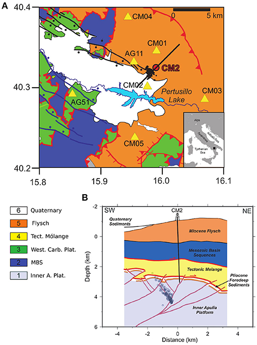
Figure 1. (A) Geologic map of the southern sector of the Val d'Agri (modified after; Improta et al., 2017). 1—Inner Apulia platform (Mesozoic–Miocene); 2—deep basin pelagic sequences (Mesozoic); 3—Western carbonate platform (Mesozoic); 4—Tectonic mólange (Late Miocene–Lower Pliocene); 5—Flysch deposits, pelagic-slope successions (Miocene); 6—Quaternary continental deposits. Red lines denote main reverse faults; blue and black thick lines denote Quaternary normal-fault systems; yellow triangles are seismic stations used in this study; the red circle is the injection well CM2. The black dots denote the epicenters of the 2006–2014 fluid injection induced earthquakes analyzed by Improta et al. (2017). (B) Schematic geologic cross-section across the CM2 well injection site. The trace of the section is reported in map with a thick line. The black circles denote the 2006–2014 fluid injection induced earthquakes located through the double-difference method by Improta et al. (2017). The schematic geologic model is modified after Buttinelli et al. (2016) and Improta et al. (2017).

FIGURE 2

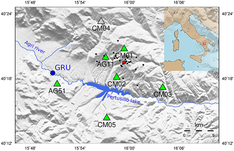
Figure 2. Seismic network (green) around the Val d'Agri oil field and Costa Molina re-injection well (red). Black dots indicate the 2015 recorded seismicity (25 events with −0.1 < M_L < 0.8.). Seismic station CM04 (gray) has not be used due to irrecoverable technical problems with the clock. Blue dot indicate the Ponte Grumento meteorological station.

FIGURE 3

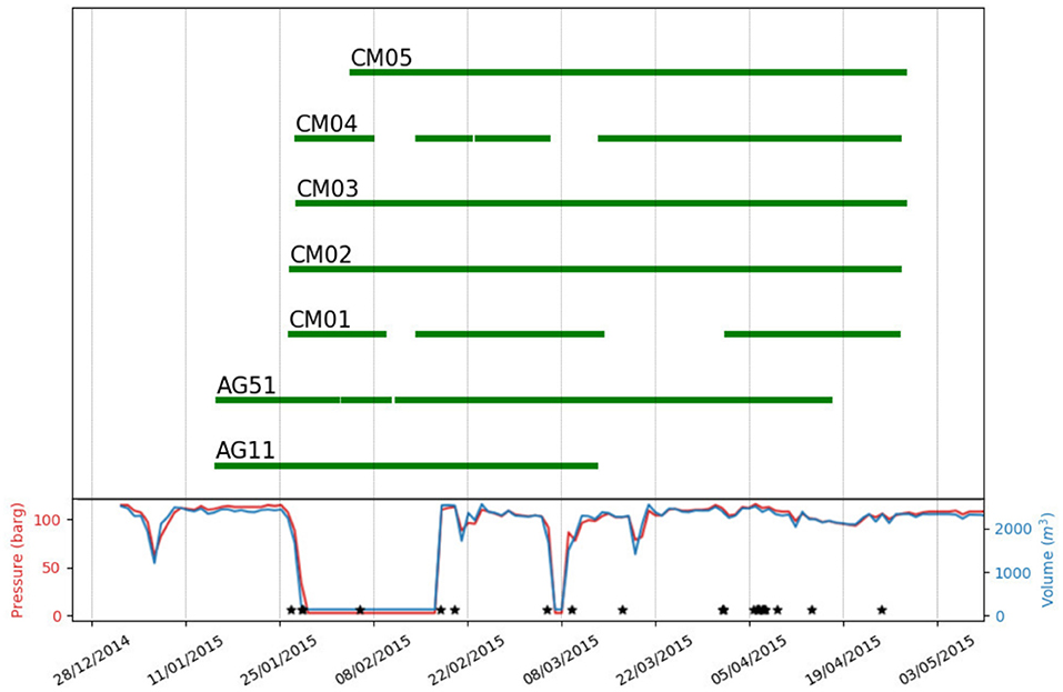
Figure 3. Data availability for each station (top panel) and daily injection data (blue: injection rate; red: maximum wellhead pressure). Black stars indicate the recorded seismicity (25 events with −0.1 < M_L < 0.8).

It is now common ground that Green's function between two seismic station can be extracted from cross-correlations (hereafter CCs) of ambient seismic noise (Lobkis and Weaver, 2001; Larose, 2006; Gouédard et al., 2008). Green's functions can then be used to retrieve a tomographic image of the crust and uppermost mantle under the region where the seismic network is deployed (Shapiro et al., 2005). This approach allows computing a static image of the seismic velocities of the subsurface with the only requirements that the noise sources are homogeneously distributed and stable in time. In practice, even though the noise sources are not homogeneously distributed, the Green's function may be achieved thanks to CCs of longer time recordings and scattering in the medium (Larose, 2006). Besides that, a temporal monitoring of the seismic velocities in the Earth crust can be performed even with an inhomogeneous noise source distribution, i.e., without a optimal reconstruction of the Green function of the medium (Hadziioannou et al., 2009), by analysing the coda of the cross-correlation functions. Coda waves are detected in the latter part of the seismogram and they can last much longer than the direct waves before reaching the background noise level (up to 10 times according to Aki, 1969). They are excited by direct waves, repeatedly scattered by small-scale heterogeneities fractures and cracks in the medium. Hence they sample the medium much more densely than direct waves, so they are more sensitive to small variations in the medium. For these reasons coda waves are also less sensitive to possible noise source changing positions (Froment et al., 2010). Noise-based monitoring has recently become an important tool to track local changes in crustal velocities and it has been successfully used in various settings: from active faults (Brenguier et al., 2008a; Zaccarelli et al., 2011), to volcanic areas (Brenguier et al., 2008b; Zaccarelli and Bianco, 2017); and geothermal reservoirs such as the St. Gallen site in Switzerland (Obermann et al., 2015), Valhall overburden in the North Sea (Mordret et al., 2014), the Reykjanes geothermal system in Iceland (Sànchez-Pastor et al., 2019).

In this study we apply the noise-based monitoring technique to detect relative variations of crustal seismic velocity in the Val d'Agri oil field using the Moving-Window Cross-Spectral analysis (Poupinet et al., 1984; Brenguier et al., 2008a; Clarke et al., 2011; Zaccarelli and Bianco, 2017). To check whether the seismic noise sources are stable in time we analyze data using the DOP-E approach (Berbellini et al., 2019). We locate our results in depth thanks to the sensitivity kernels computed from the velocity model of this region (Valoroso et al., 2009) using a modal summation approach by Herrmann (2013). Interestingly, we find a strong correlation of the velocity trend to the hydrological level of the Agri river. Hence, we remove the contribution of hydrological parameter changes to the crustal velocity changes and we interpret the residual results in terms of local diffusivity of the medium.

2. Geological Setting

The study area is located in the Lucania arc of the NE-verging southern Apennines thrust-and-fold belt. The upper crust includes NW-trending Mio-Pliocene thrusts and related folds deforming Meso-Cenozoic shelf carbonate and basin sequences (Mazzoli et al., 2001). The subsurface is structured into two main units: (i) an upper pile of rootless thrust sheets formed by carbonate platform, deep pelagic, and flysch sequences 2–4 km thick, (ii) the 5–7 km thick Inner Apulia carbonate Platform (IAP) deformed during Late Pliocene—Early Pleistocene by deeply rooted, steep reverse faults (Figure 1; Mazzoli et al., 2001). The IAP hosts the reservoir of the Val d'Agri oil field with hydrocarbon and brines trapped into thrust-related anticlines formed by low-porosity, strongly fractured limestone (Figure 1). The cap rocks consist of low-permeability mudstones and siltstones that form a Pliocene tectonic mèlange up to 1 km thick and tectonically sandwiched between the upper rootless nappes and the IAP (Figure 1; Shiner et al., 2004).

In the survey area, several oil wells reached the Apulian carbonate reservoir at 2–3 km depth b.s.l. (Improta et al., 2017). The geologic units drilled by the injection well CM2 include from top to bottom (Buttinelli et al., 2016): (i) clay-sandstone alternances and marly-calcareous strata referable to Miocene flysch (from 1,045 to 468 m b.s.l.), (ii) deep basin Mesozoic sequences also including Cretaceous shales (468–1,490 m b.s.l.), (iii) mudstones and siltstones sequences of the Pliocene tectonic mèlange (1,490–2,712 m b.s.l.), (iv) foredeep Pliocene clays and sandstones (2,712–2,821 m b.s.l.), and (v) fractured high permeability Miocene-Cretaceous limestone of the IAP (2,821–3,071 m b.s.l.). The presence of very thick and very-low permeability clayey sequences at the top of the IAP hinders the hydraulic communication between the rootless nappes and the carbonate reservoir (Improta et al., 2017).

Co-produced salt water has been re-injected in the high permeability Cretaceous limestone of the Apulian reservoir through the CM2 wellbore. Due to the alternance of low permeability clays with medium permeability sandstones and marly-limestones, the underground water circulation in the injection area is characterized by a near-surface, thin aquifer developed in the weathered flysch deposits and fed by rainfall and by deeper, compartmentalized, and overlapping aquifers developed in the medium-porosity and/or fractured sandy and calcareous beds. The quasi-instantaneous onset of microseismicity located under the well was explained in terms of rapid propagation of pore-pressure perturbation from the wellbore to an inherited Pliocene reverse fault that is confined within the reservoir (Figure 1; Buttinelli et al., 2016; Improta et al., 2017). The fault is located to the SW of the well CM2 and optimally oriented to slip in the present extensional stress field. Permeability of the Apulian carbonate reservoir has been estimated in the order of k = 10⁻¹³m² from hydraulic well tests, production data and diffusivity analysis on the injection induced seismicity (Chelini et al., 1997; Improta et al., 2015).

3. Data

The 2015 passive seismic survey was carried out from January 26th to April 27th. During this experiment five stations (Figure 2) were installed within 10 km from the CM2 well (named CM01–CM05). Two additional INGV temporary stations, AG11 and AG51, that were operating in the injection area before the suspension of disposal operations, complete the 7-stations network that we use here to monitor possible changes in relative crustal velocities. The stations were equipped with Reftek130 acquisition systems coupled with Lennartz 3-D 5 s sensors, and recorded at a sampling rate of 125 Hz. We discard station CM04 because of irrecoverable technical problems with the clock. Apart from CM02 and AG11, the seismic stations used in this study and surrounding the well CM2 were installed on Miocene flysch deposits (Figure 1). Seismic station CM02 was installed in the valley on Quaternary continental sediments about 100 m thick that overlay the Miocene flysch. The seismic station AG51 was deployed on Mesozoic fractured limestone belonging to the uppermost rootless nappe. Due to the strong fracturing, these terrains are characterized by a poorly known carbonate basal aquifer. While seismic stations are missing in the NE region from CM2, the azimuthal coverage of the station couples is quite complete. Five out of seven stations (CM01-05) have been installed the same day the injection was halted (see Figure 3; injection data from De Gori et al., 2015), therefore recorded data do not allow investigating the status of the system before the injection stop. This would have been very important to better interpret the velocity variations after the injection re-start.

4. Method

4.1. Polarization Analysis

The CCs temporal analysis is based on the assumption that the ambient noise sources are stable in time (Hadziioannou et al., 2009). In order to verify this assumption we perform a polarization analysis using the DOP-E method (Berbellini et al., 2019). This method filters the portion of ambient noise containing the most polarized signals and extract different observables such as the ellipticity of Rayleigh waves. Moreover, it is able to measure the back azimuth of the incoming signal, a useful tool to study the ambient noise sources. We apply this scheme to our data and we show in Figure 4 the overall polarization for four sample stations. We observe here that for the majority of the stations the noise sources are located on a direction coming from the south-west. This is more evident in the frequency band 0.5–1.0 Hz, while in the frequency band 0.1–0.5 Hz the signals are more diffuse, but still in the south-west direction. Only station CM03 shows a different incoming azimuth, with a peak at around 315^o. This can be due to the particular local geology in the area surrounding the station. Pischiutta et al. (2014) measured polarization of signals from the analysis of local microseismicity. They observed an overall NE-SW distribution and an anomalous polarization in the CM03 area (they used records from temporary station AG10 located 300 m far from CM03). Our results are then in good agreement with previous findings. The presence of a non homogeneous spatial distribution of the noise sources cause asymmetrical CC functions, as we can observe in Figure 5, but such an uneven distribution of the sources does not prevent us from using our approach, as long as the noise source distribution is stable in time. We verify its stability by repeating the DOP-E analysis on data stacked every 15 days. Station AG51 showed problems on one of the horizontal components, so the polarization analysis was not possible on this station. Since the vertical component shows good quality data and in the followings we perform CC analysis only on this component, we keep the station for the main analysis. All the other stations (see Supplementary Figures 1–5) showed a main direction for the incoming noise sources which is quite stable in time during the recording period. Moreover, it is noteworthy that, as already mentioned, we take into account only the coda of the cross-correlation functions, thus avoiding its central part, which is more sensitive to the changing position of the noise sources (Froment et al., 2010).

FIGURE 4

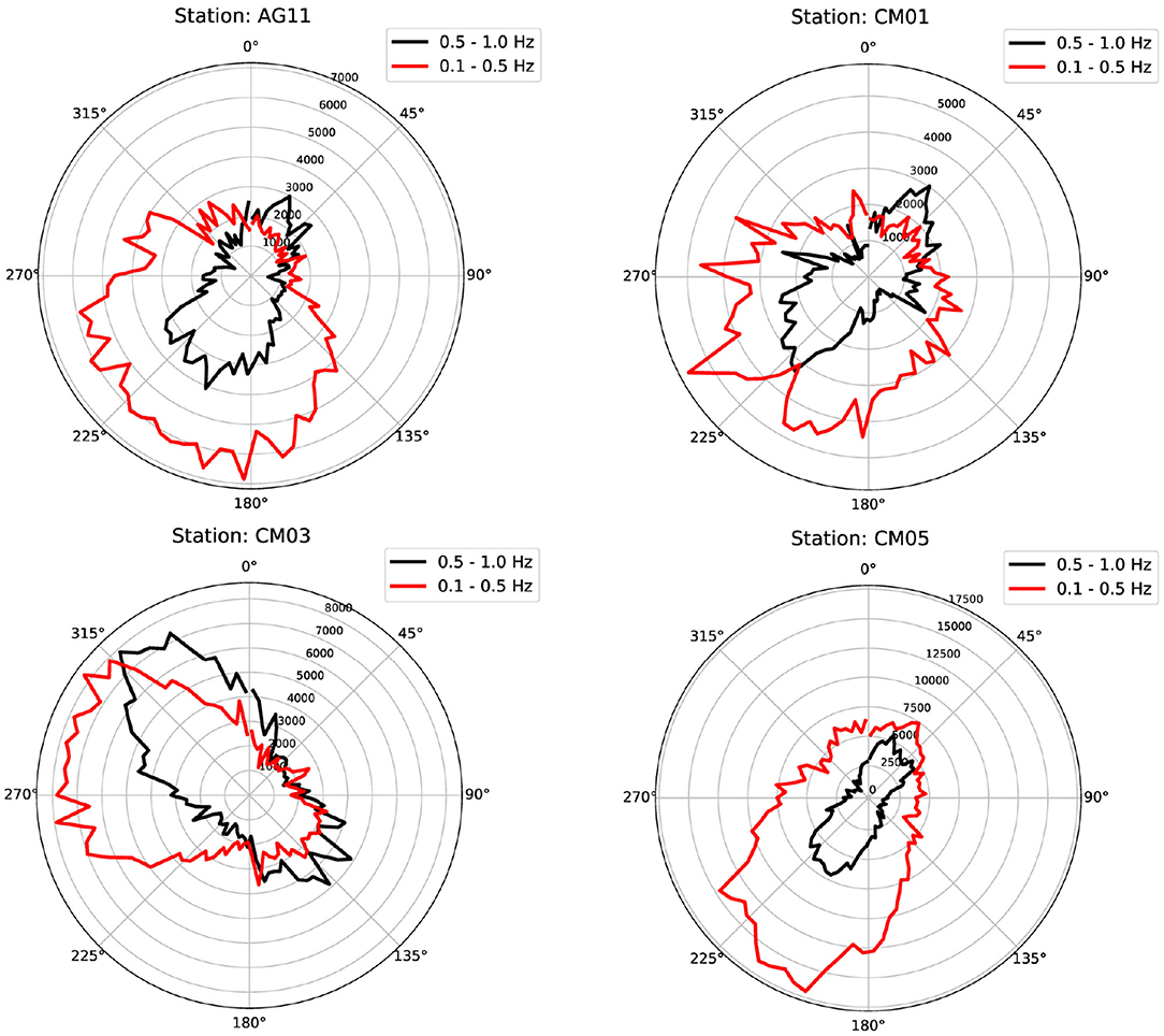
Figure 4. Azimuthal source distribution in all the period for 4 sample stations measured using the DOP-E approach (Berbellini et al., 2019) in two different frequency bands, 0.5–1.0 Hz (black line) and 0.1–0.5 Hz (red line).

FIGURE 5

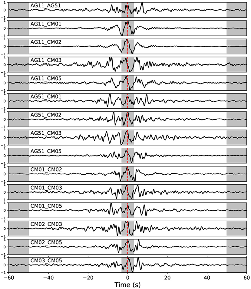
Figure 5. Reference cross-correlations for all the station pairs available. Gray areas are the part of the signal excluded from the analysis.

4.2. Pre-processing

We compute the relative variations of crustal velocities using the Moving-Window Cross-Spectral analysis (Poupinet et al., 1984; Brenguier et al., 2008a):

we fill the data gaps through a linear interpolation. We apply the filling if the gaps last <20% of the 1 h length used as quantum of data. Then we apply a signal whitening in the frequency domain in the frequency band 0.1–1.0 Hz, as proposed by Zaccarelli et al. (2011) and a 1-bit normalization in the time domain. Finally we compare a reference cross-correlation (CC-ref) of ambient noise with the cross-correlations measured for each time interval (CC-cur). The whole analysis is performed in the frequency band 0.1–1.0 Hz.

4.3. Reference and Current Cross-Correlations

As a first step after this pre-processing we define the reference CC for each station pair by computing the cross-correlation for the whole available recordings by stacking all 1 h CCs computed on the entire recordings in the frequency band 0.1–1.0 Hz. In Figure 5, we show all the reference cross correlations used in this study.

Hence we compute the current cross-correlation over subsequent time intervals along the whole dataset, stacked over a certain number of days. The number of days that we are using for the stacking is quite important, since if the time interval is too short, then the CC-cur will be too different from the reference CC and the measurement will be unstable. On the opposite, if the stacking time is too long, the current CC will be very similar to the reference but the variations will loose time resolution. In order to select the optimal time interval we compute the mean correlation coefficients between the reference and current CC for 4 sample station pairs using different number of stacking days (see Zaccarelli et al., 2011). We choose a convergence test which is quantitative compared to the qualitative method chosen by D'Hour et al. (2015) (visual inspection). Our test is actually equivalent to Nuez et al. (2020) that looks at the similarity evolution between CCref and CCcur with the increasing stacking length. Results are shown in Figure 6. Here we notice that the mean correlation coefficient increases with the number of days and, as expected, tends asymptotically to 1. On the basis of this plot we choose 15 days as a good compromise between similarity of the CC and time resolution Our CC-cur's are then computed every day and they are computed as the stacking of the previous 15 days.

FIGURE 6

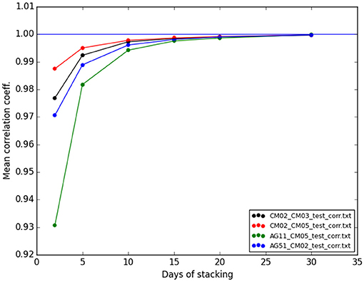
Figure 6. Test to select the optimal number of days of stacking. Mean correlation coefficient between CC current and reference for four sample couples as a function of the number of stacking days.

4.4. Moving Window Cross-Spectral Method

In order to measure the relative crustal velocity variation in time, we apply the Moving Window Cross-Spectral approach described by Clarke et al. (2011). This approach estimates the time-shift between the CC-cur (relative to 15 days of stacking) and the CC-ref (relative to all the period) waveforms. Time shift is directly related to the relative velocity variation following the relationship:

$\begin{array}{ll}\frac{\tau }{t}=-\frac{\Delta v}{v}& (1)\end{array}$

where τ is the time-shift, t is the time, v is the crustal velocity and Δv its variation. We discard a time interval of 3 s around 0 (gray areas in Figure 5), estimated as an average propagation time of surface waves between each station in the region (Improta et al., 2017). We also exclude cross-correlations after 50 s, since after this interval the signal is lost in the background noise. In order to stabilize the measurements we include in the computation only the CC-cur with a correlation coefficient relative to the CC-ref larger than 0.85. We merge together all time-shifts estimated for each couple by computing their median values before estimating the final Δv/v, in order to get a picture of the mean time evolution of relative velocities variations in the whole medium included in the network. The velocity variations are defined in depth by the penetration of surface waves in the frequency band considered, estimated by the sensitivity kernels described in the following.

5. Results

5.1. Description of the Results

Results are shown in Figure 7. Here we plot the relative velocity variation (top), the correlation coefficient between currents and reference for all the station pairs (central), and the daily injected volume and maximum well-head pressure (bottom panel; De Gori et al., 2015). We can observe a clear increase in relative velocity in the second half of February, followed by a decrease between the end of February and the beginning of March. After this, Δv/v tends to a slightly larger value that remains more stable afterwards, with variations of about ±0.02%. Observing the correlation coefficient plot (central panel) we notice a general low correlation in the very first part of the period, followed by a strong increase in correlation corresponding to the injection restart. Then, the correlation coefficient does not vary substantially. We observe a decrease for couples containing AG11 at the end of the recording period, at the same time of occurrence of some local earthquakes nearby. These two factors do not find any correspondence in Δv/v variations. To complete the analysis we split the frequency band into two segments, 0.1–0.5 and 0.5–1.0 Hz. With this test we want to verify if the high frequency waves, sensitive to shallower depths show different trends compared to lower frequencies, sensitive to deeper structures. Results are shown in Supplementary Figure 6. Here we observe that both the frequency bands show the same trend observed using the whole band, but the lower frequencies show much larger errors and an overall larger instability. Higher frequency at the contrary show very similar behavior to the results based on the whole frequency range.

FIGURE 7

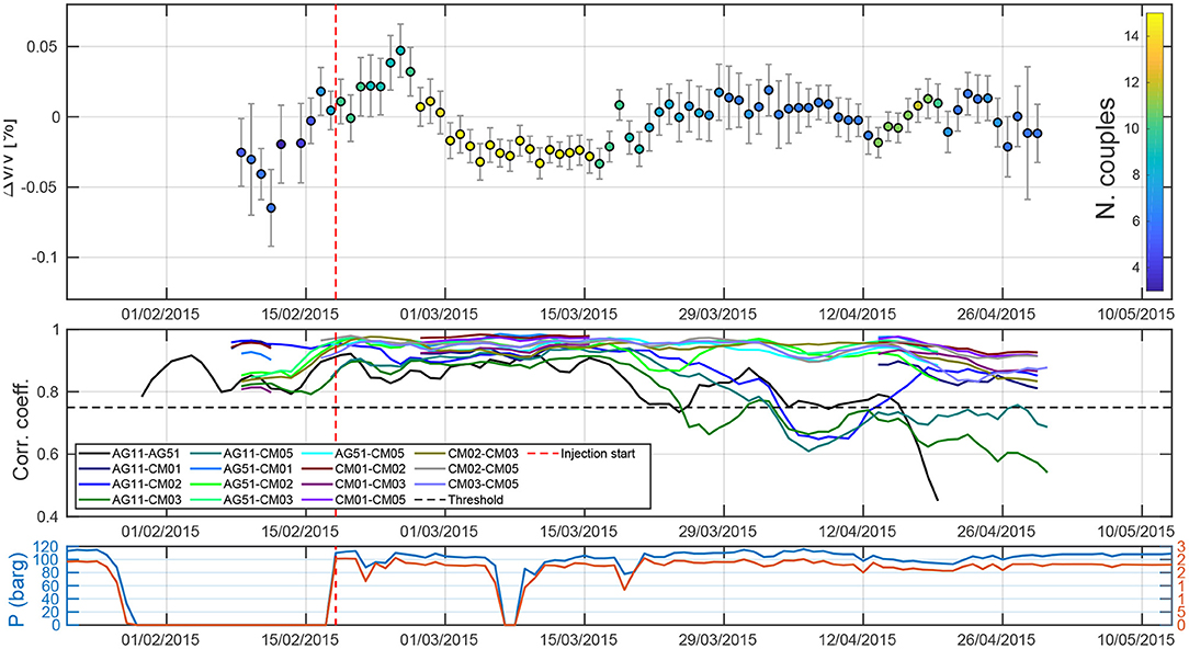
Figure 7. (Top) Percentual crustal velocities variations as a function of time in the frequency band 0.1–1.0 Hz. Colors represent the number of station couples available at each time. (Middle) Correlation coefficient between currents and reference for each couple as a function of time. We exclude from the computation the data with a correlation coefficient lower than 0.75 (black dotted line). (Bottom) Injection daily pressure (red) and rate (blue) from De Gori et al. (2015).

5.2. Sensitivity Kernels

In order to better constrain the results in depth we compute the sensitivity kernels for phase and group velocities using the 1D, flat layered model for the Val D'Agri region by Valoroso et al. (2009). Kernels show the sensitivity of the observable at the surface (i.e., phase velocity) to variations of a crustal parameter (v_S, v_P, and density) with depth. We compute the sensitivity kernels numerically using a modal summation approach (Herrmann, 2013): we divide each flat layer into 0.1 km thick sub-layers. We increment and decrement v_S at each depth by 10% and for the two models we compute the phase velocity using the modal summation approach. For each sub-layer we compute the derivative using the finite differences approach.

Results are shown at Figure 8. We notice that at the higher frequencies (0.5–1 Hz), that mainly contribute to our results, the sensitivity is stronger and confined in the top 5 km, while it decreases and becomes deeper at lower frequencies. At 1Hz the sensitivity is an order of magnitude bigger than 0.1Hz, but it does not extend below 3 km depth. Co-produced saltwater is re-injected between 2.8 and 3.0 km depth b.s.l. within the liquid-bearing saturated reservoir. In the southern sector of the oil field, the IAP culminations are at 1.8–2.8 km depth b.s.l. and the reservoir thickness is 3–4 km (Improta et al., 2017). Therefore, the relative velocity changes resolved by the high frequency data (0.5–1.0 Hz) may be confined in the top 5 km of the crust and can be reasonably associated to the fractured carbonate reservoir and to the overlying thrust sheets.

FIGURE 8

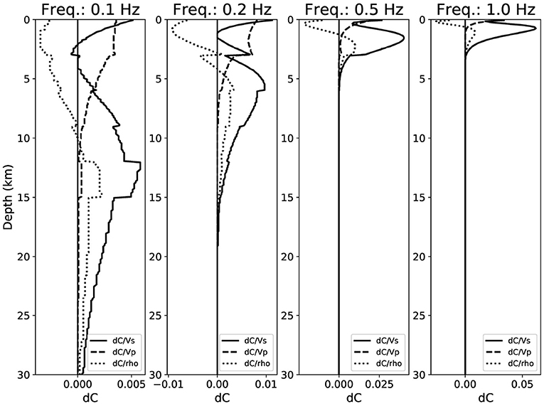
Figure 8. Sensitivity kernels for the phase velocity as a function of v_S, v_P, and density computed using a modal summation approach (Herrmann, 2013) using the 1D model of the Val d'Agri area by Valoroso et al. (2009).

6. Rainfall and Hydrometric Comparison

Recent studies showed that water table fluctuations in the top hundreds meters can cause variations in the crustal velocities that can be successfully detected by ambient noise monitoring (Sens-Schönfelder and Wegler, 2006; Rivet et al., 2015 and more recently Lecocq et al., 2017; Wang et al., 2017; Clements and Denolle, 2018; Liu et al., 2020; Poli et al., 2020). They observed that these variations can be large enough to cover other minor fluctuations due to secondary mechanisms. For this reason we first want to verify if the relative velocity variations shown in Figure 7 are due to hydrological effects. We compare the observed velocity trend with three datasets from the regional civil protection office (downloaded from http://centrofunzionalebasilicata.it; see Supplementary Figure 7): daily rainfall (that we have cumulated by 15 days before comparison to our measurements) recorded at the nearest meteorological station (Ponte Grumento, GRU in Figure 2), river Agri hydrometric level, recorded at the same location and the water level of the Pertusillo artificial Lake (Figure 2). The first two (sign-reversed) time series are very similar to the dv/v trend, while the Pertusillo charge/discharge rate is definitely acting at longer period compared to the previous observables. We try to remove the contribution of precipitation to the observed velocity variations. Following the method proposed by Wang et al. (2017), we firstly compute the pore pressure variations induced by precipitations. Then we use it to compute the synthetic velocity variation due to rainfall. We observe that predicted synthetic velocity variations are much smaller than the observed ones, so we conclude that this method is not suitable to remove the contribution of rainfall to crustal velocity variations. Furthermore, we observe that the parameter that best fits the velocity variations is the hydrometric level of the Agri river (Supplementary Figure 7). We observe that the main dv/v maximum peak around the 24th of February fits well with the minimum of the hydrometric level (sign-reversed in the plot). The fit is quite good until the 8th of April, then the two trends do not fit well. The anti-correlation is quite clear: higher hydrometric levels correspond to slower crustal velocities. In fact, the CC codas at the frequencies 0.1–1.0 Hz are mainly composed by surface waves, meaning that we measure dv/v of multiple scattered coda waves, which decrease their velocity in the presence of fluids. The Agri river hydrometric level can be considered as a proxy of the total water storage in the valley, as it depends not only on the rainfalls but also on the total underground water amount. Consequently, the observed variation of shear-wave velocity can be interpreted in terms of variations in the aquifers hosted in the medium-permeability intervals (i.e., fractured sandstone and marly-limestones) of the thick Miocene flysch deposits outcropping in the survey area.

7. Discussion

The velocity variations that we observe are mainly due to hydrological effects (rainfall, snow melting.) hiding any possible velocity variations due to the water injection restart.

In order to verify if it is still possible to observe a velocity change due to the produced water injection restart, we remove the hydrometric trend from the velocity time-series. We de-mean and normalize both the dv/v and hydrometric trends to make them comparable. Finally we deconvolve the velocity time-series with the hydrometric level and plot the deconvolution reminder (Figure 9). Here we observe that the deconvolved velocity trend still shows a velocity peak in 24th February 2015, which is smaller than the original one. This could be possibly due to water injection restart, which happened 7 days before (18 February 2015). Other minor peaks are observed around the 8th of March and the 17th of March (Figure 9 bottom panel) which could be possibly linked to minor injection reductions (see Figure 7). Since the injection reductions are very small and the two peaks are quite isolated, we prefer not to over-interpret them as effect of injection variations.

FIGURE 9

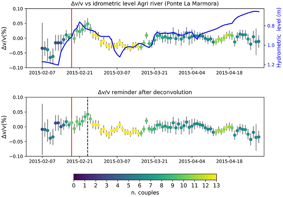
Figure 9. (Top) Percentual crustal velocities variations as a function of time (dots) compared to the idrometric level of the Agri river (blue line, reversed y axes). (Bottom) Percentual crustal velocities variations after removing the Agri river idrometric level. Red line: produced water injection restart. Black dotted line: dv/v maximum.

We evaluate if the observed peak has some statistical significance with respect to the other peaks observed in the dv/v time series. With this aim we use a z-test to assess, for each dv/v point in the time series, if a random sample generated from a Normal distribution with mean dv/v and standard deviation the double of the respective formal error can be drawn from a reference Normal distribution characterized by the mean and the standard deviation (considering the double standard error of that point as well) of the maximum peak. It is worth noting that assuming the double of the formal error to set the standard deviation is a conservative choice justified by the fact that the MWCS analysis tends to underestimate the errors (Clarke et al., 2011). In practice, we take the peak value (i.e., the one on 24th February 2015) and the related uncertainty as a reference set of parameters, and use the z-test to compare this reference distribution with samples drawn from the distributions defined for each of the other points. We find that the probability that any of the generated samples is drawn from the peak distribution is very low (p-values < < 1% in all the cases), indicating that the observed peak is significantly higher respect to all the other points. Similar results are obtained using non parametric tests (as e.g., the Kolmogorov-Smirnov test).

Knowing that the 24th February 2015 peak in dv/v is statistically significant, we intend to investigate on its possible relationship with the water injection restart. We start by computing the medium diffusivity, assuming that the observed velocity decrease is due to the propagation of produced water from the Costa Molina injection, restarted on 18th February 2015. Then we want to verify if the obtained diffusivity is compatible with the value computed from independent studies based on the seismicity induced by the first injection tests in 2006 and on hydraulic well tests in the hydrocarbon reservoir (Chelini et al., 1997; Improta et al., 2015). Hence we measure the delay time from the injection start (7 ± 1 days) and the average distance between the stations and the injection well (6.40 km). We then compute the medium diffusivity, using the equation (Shapiro, 2015):

$\begin{array}{ll}D=\frac{R_T^2}{4\pi t}& (2)\end{array}$

where R_T is radius of the triggering front (in this case the average station-well distance) and t is the delay time from the injection start to the time when Δv/v curves reach their maxima. We compute a diffusivity value of 5m²/s. We repeat the calculation using for R_T the average station-well distance for the three closest stations (2.82 km for stations AG11, CM01, and CM02) obtaining a diffusivity value of 1m²/s.

We compute both values aiming at a diffusivity range definition, since we do not have the spatial resolution to precisely locate dv/v in the map. The peak in dv/v means that a crustal variation has occurred in the medium included in the seismic network, and either it is very localized but big enough to be visible (not canceled) from all the stations, or it is small but spread out over all station locations. We then estimate the time evolution of the triggering front R_T given the observed diffusivity values (Table 1) using the Equation (2). Results are shown in Figure 10. Here we also plot the seismicity observed in June 2006 during the first injection tests (Improta et al., 2017), plotted as a function of distance from the CM2 well and time after the first injection test initiated the 1st June. The 2006 seismicity has been demonstrated to be induced by the first injection tests (Improta et al., 2017). Here we focus on the first events only to verify if the delay times observed in the 2006 induced sequence are compatible with the two triggering fronts obtained from the two diffusivity values. We observe that the first events triggered in 2006 fall in the range between the two triggering fronts estimated from the diffusivity range based on our observations. The first injection tests in 2006 activated a fault ≈ 1.7km far from the well bottom (Improta et al., 2015), with a delay time in the range expected from the diffusivity values we obtained here. No other faults slip seismically during the injection tests in 2006 (Improta et al., 2015), so it is not possible to compare our results to other seismic swarms. From this experiment we can conclude that the peak observed in 24th February 2015 could possibly be due to the produced water injection re-start, since the diffusivity estimated from its delay time is in the same order of magnitude of what we observe from other independent measurements, such as 2006 induced seismicity, but other studies should be done to confirm this hypothesis.

TABLE 1

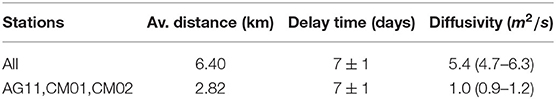
Table 1. Average inter-station distance, observed peak delay time and diffusivity computed from Improta et al. (2017).

FIGURE 10

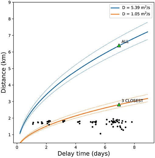
Figure 10. Colored lines: triggering front computed from diffusivity values estimated from Equation (2) for station AG11 and CM02 (green triangles). Diffusivity values are reported in the legend. Black dots: seismicity recorded in June 2006 during the first injection tests (Improta et al., 2017), plotted as a function of delay time and distance from the injection well.

The obtained diffusivity values are compatible with the expected ones in such a geological setting. For instance, diffusivity values in the range 0.3–2 m²/s has been observed in many different regions (Costain et al., 1987; Rothert et al., 2003; Costain, 2008; Costain and Bollinger, 2010). Also, Christiansen et al. (2007) estimated a diffusivity value of ≈ 2m²/s for the Parkfield area at 5 km depth. Finally, Hainzl et al. (2006) found a diffusivity equals to 3.3 ± 0.8m²/s for rain-induced events in Bavaria, Germany.

8. Conclusions

We monitored crustal velocity changes in a time period including the restart of produced water re-injection at the CM2 well in the Val d'Agri oil field (southern Italy) from noise-based monitoring. We used continuous recordings from a temporary seismic array deployed during the first out of 22 days pause of the injection in January–February 2015.

We observed that the relative velocity time-series match well with the hydrometric level of the Agri river. Hence we hypothesize that the observed velocity changes are mainly due to variations of water storage in the shallow aquifers developed in the thick, Miocene flysch deposits that crop out in the survey area. This effect can hide smaller variations due to the produced water injection restart in the Costa Molina 2 well.

We removed by deconvolution the hydrometric level time-series of the Agri river from the relative velocity change and we noticed that the peak observed 7 days after injection restart is lower but still visible.

Using this time delay we compute the medium diffusivity to verify if the observed peak can be related to the water injection re-start and finding values in the range 1–5 m^2/s, which are compatible with the delay time of the induced seismicity measured in 2006 after the first injection tests (Improta et al., 2015) and with hydraulic properties of similar geological settings.

Our results demonstrate that observed crustal velocity changes are often mainly due to changes in the total underground water storage. This can totally hide the weaker effects due to produced water injection and can not be neglected when monitoring with ambient noise cross-correlations.

Data Availability Statement

Seismic data from stations CM01-05 are from a temporary deployment and they are available upon request by emailing to: luigi.improta@ingv.it. Data from stations AG11 and AG51 are provided by INGV and are available from ORFEUS-EIDA data center (http://www.orfeus-eu.org/data/eida).

Author Contributions

AB carried out the measurements, wrote the manuscript, and coordinated the co-authors. LZ provided the original scripts, supervised the measurement process, and contributed with the interpretation of the results. LF provided the original codes and supervised their setting. LI wrote the geological setting section, interpreted the results from a geological point of view, and planned the seismic survey and contributed to the stations deployment. PD carried out the instrument installation and provided data. AG carried out the diffusivity computation and helped with the statistical assessment of the results. AM coordinated the whole project, supervised the interpretation of the results, and raised funds. All authors contributed to the article and approved the submitted version.

Funding

This study benefitted from support by Clypea, the Innovation Network for Future Energy financed by the Italian Ministry of Economic Development, Direzione Generale per le Infrastrutture e la Sicurezza dei Sistemi Energetici e Geominerari (DG ISSEG); and by Regione Basilicata (Italy) in the framework of the Protocollo d'Intesa: Accordo per la sperimentazione delle Linee Guida in Val d'Agri.

Conflict of Interest

The authors declare that the research was conducted in the absence of any commercial or financial relationships that could be construed as a potential conflict of interest.

The handling Editor APR declared a past co-authorship with one of the authors LI.

Acknowledgments

Well injection data are collected by ENI and archived and made accessible upon request by the regional regulatory agency (Basilicata Region). We also thank the two reviewers for their helpful suggestions and comments that greatly improved this manuscript.

Supplementary Material

The Supplementary Material for this article can be found online at: https://www.frontiersin.org/articles/10.3389/feart.2021.626720/full#supplementary-material

References

Aki, K. (1969). Analysis of the seismic coda of local earthquakes as scattered waves. J. Geophys. Res. 74, 615–631. doi: 10.1029/JB074i002p00615

PubMed Abstract | CrossRef Full Text | Google Scholar

Berbellini, A., Schimmel, M., Ferreira, A. M., and Morelli, A. (2019). Constraining S -wave velocity using Rayleigh wave ellipticity from polarization analysis of seismic noise. Geophys. J. Int. 216, 1817–1830. doi: 10.1093/gji/ggy512

CrossRef Full Text | Google Scholar

Brenguier, F., Campillo, M., Hadziioannou, C., Shapiro, N. M., Nadeau, R. M., and Larose, E. (2008a). Postseismic relaxation along the San Andreas fault at Parkfield from continuous seismological observations. Science 321, 1478–1481. doi: 10.1126/science.1160943

PubMed Abstract | CrossRef Full Text | Google Scholar

Brenguier, F., Shapiro, N., Campillo, M., Ferrazzini, V., Duputel, Z., Coutant, O., et al. (2008b). Toward forecasting volcanic eruptions using seismic noise. Nat. Geosci. 1, 126–130. doi: 10.1038/ngeo104

CrossRef Full Text | Google Scholar

Buttinelli, M., Improta, L., Bagh, S., and Chiarabba, C. (2016). Inversion of inherited thrusts by wastewater injection induced seismicity at the Val d'Agri oilfield (Italy). Sci. Rep. 6:37165. doi: 10.1038/srep37165

PubMed Abstract | CrossRef Full Text | Google Scholar

Chelini, V., Sartori, G., Ciammetti, G., Giorgioni, M., and Pelliccia, A. (1997). “Enhancing the image of the Southern Apennines,” in Reservoir Optimization Conference (Milan: Schlumberger).

Christiansen, L. B., Hurwitz, S., and Ingebritsen, S. E. (2007). Annual modulation of seismicity along the san andreas fault near parkfield, ca. Geophys. Res. Lett. 34:L04306. doi: 10.1029/2006GL028634

CrossRef Full Text | Google Scholar

Clarke, D., Zaccarelli, L., Shapiro, N. M., and Brenguier, F. (2011). Assessment of resolution and accuracy of the Moving Window Cross Spectral technique for monitoring crustal temporal variations using ambient seismic noise. Geophys. J. Int. 186, 867–882. doi: 10.1111/j.1365-246X.2011.05074.x

CrossRef Full Text | Google Scholar

Clements, T., and Denolle, M. A. (2018). Tracking groundwater levels using the ambient seismic field. Geophys. Res. Lett. 45, 6459–6465. doi: 10.1029/2018GL077706

CrossRef Full Text | Google Scholar

Costain, J. K. (2008). Intraplate seismicity, hydroseismicity, and predictions in hindsight. Seismol. Res. Lett. 79, 578–589. doi: 10.1785/gssrl.79.4.578

CrossRef Full Text | Google Scholar

Costain, J. K., and Bollinger, G. A. (2010). Review: research results in hydroseismicity from 1987 to 2009. Bull. Seismol. Soc. Am. 100, 1841–1858. doi: 10.1785/0120090288

PubMed Abstract | CrossRef Full Text | Google Scholar

Costain, J. K., Bollinger, G. A., and Speer, J. A. (1987). Hydroseismicity: a hypothesis for the role of water in the generation of intraplate seismicity. Geology 15, 618–621. doi: 10.1130/0091-7613(1987)15<618:HHFTRO>2.0.CO;2

CrossRef Full Text | Google Scholar

De Gori, P., Improta, L., Moretti, M., Colasanti, G., and Criscuoli, F. (2015). “Monitoring the restart of a high-rate wastewater disposal well in the Val d'Agri oilfield (Italy),” in AGU Fall Meeting Abstracts, (Cambridge), S13B–2802.

Google Scholar

D'Hour, V., Schimmel, M., Nascimento, A., Ferreira, J., and Neto, H. (2015). Detection of subtle hydromechanical medium changes caused by a small-magnitude earthquake swarm in ne Brazil. Pure Appl. Geophys. 173, 1097–1113. doi: 10.1007/s00024-015-1156-0

CrossRef Full Text | Google Scholar

Froment, B., Campillo, M., Roux, P., Gouédard, P., Verdel, A., and Weaver, R. L. (2010). Estimation of the effect of nonisotropically distributed energy on the apparent arrival time in correlations. Geophysics 75, SA85–SA93. doi: 10.1190/1.3483102

CrossRef Full Text | Google Scholar

Gouédard, P., Stehly, L., Brenguier, F., Campillo, M., Colin de Verdiére, Y., Larose, E., et al. (2008). Cross-correlation of random fields: mathematical approach and applications. Geophys. Prospect. 56, 375–393. doi: 10.1111/j.1365-2478.2007.00684.x

CrossRef Full Text | Google Scholar

Hadziioannou, C., Larose, E., Coutant, O., Roux, P., and Campillo, M. (2009). Stability of monitoring weak changes in multiply scattering media with ambient noise correlation: laboratory experiments. J. Acoust. Soc. Am. 125:2654. doi: 10.1121/1.3125345

PubMed Abstract | CrossRef Full Text | Google Scholar

Hainzl, S., Kraft, T., Wassermann, J., Igel, H., and Schmedes, E. (2006). Evidence for rainfall-triggered earthquake activity. Geophys. Res. Lett. 33:L19303. doi: 10.1029/2006GL027642

CrossRef Full Text | Google Scholar

Herrmann, R. B. (2013). Computer programs in seismology: an evolving tool for instruction and research. Seismol. Res. Lett. 84, 1081–1088. doi: 10.1785/0220110096

CrossRef Full Text | Google Scholar

Improta, L., Bagh, S., De Gori, P., Valoroso, L., Pastori, M., Piccinini, D., et al. (2017). Reservoir structure and wastewater-induced seismicity at the Val d'Agri oilfield (Italy) shown by three-dimensional V p and V p /V s local earthquake tomography. J. Geophys. Res. 122, 9050–9082. doi: 10.1002/2017JB014725

CrossRef Full Text | Google Scholar

Improta, L., Valoroso, L., Piccinini, D., and Chiarabba, C. (2015). A detailed analysis of wastewater-induced seismicity in the Val d'Agri oil field (Italy). Geophys. Res. Lett. 42, 2682–2690. doi: 10.1002/2015GL063369

CrossRef Full Text | Google Scholar

Larose, E. (2006). Mesoscopics of ultrasound and seismic waves: application to passive imaging. Ann. Phys. 31, 1–126. doi: 10.1051/anphys:2007001

CrossRef Full Text | Google Scholar

Lecocq, T., Longuevergne, L., Pedersen, H. A., Brenguier, F., and Stammler, K. (2017). Monitoring ground water storage at mesoscale using seismic noise: 30 years of continuous observation and thermo-elastic and hydrological modeling. Sci. Rep. 7:14241. doi: 10.1038/s41598-017-14468-9

CrossRef Full Text

Liu, C., Aslam, K., and Daub, E. (2020). Seismic velocity changes caused by water table fluctuation in the new Madrid seismic zone and Mississippi embayment. J. Geophys. Res. 125:e2020JB019524. doi: 10.1029/2020JB019524

CrossRef Full Text | Google Scholar

Lobkis, O. I., and Weaver, R. L. (2001). On the emergence of the green's function in the correlations of a diffuse field. J. Acoust. Soc. Am. 110, 3011–3017. doi: 10.1121/1.1417528

PubMed Abstract | CrossRef Full Text | Google Scholar

Mazzoli, S., Barkham, S., Cello, G., Gambini, R., Mattioni, L., Shiner, P., et al. (2001). Reconstruction of continental margin architecture deformed by the contraction of the lagonegro basin, Southern Apennines, Italy. J. Geol. Soc. 158, 309–319. doi: 10.1144/jgs.158.2.309

CrossRef Full Text | Google Scholar

Mordret, A., Shapiro, N. M., and Singh, S. (2014). Seismic noise-based time-lapse monitoring of the valhall overburden. Geophys. Res. Lett. 41, 4945–4952. doi: 10.1002/2014GL060602

CrossRef Full Text | Google Scholar

Nuez, E., Schimmel, M., Stich, D., and Iglesias, A. (2020). Crustal velocity anomalies in Costa Rica from ambient noise tomography. Pure Appl. Geophys. 177, 941–960. doi: 10.1007/s00024-019-02315-z

CrossRef Full Text | Google Scholar

Obermann, A., Kraft, T., Larose, E., and Wiemer, S. (2015). Potential of ambient seismic noise techniques to monitor the St. Gallen geothermal site (Switzerland). J. Geophys. Res. B 120, 4301–4316. doi: 10.1002/2014JB011817

CrossRef Full Text | Google Scholar

Pischiutta, M., Pastori, M., Improta, L., Salvini, F., and Rovelli, A. (2014). Orthogonal relation between wavefield polarization and fast S wave direction in the val d'agri region: An integrating method to investigate rock anisotropy. J. Geophys. Res. 119, 396–408. doi: 10.1002/2013JB010077

CrossRef Full Text | Google Scholar

Poli, P., Marguin, V., Wang, Q., D'Agostino, N., and Johnson, P. (2020). Seasonal and coseismic velocity variation in the region of l'aquila from single station measurements and implications for crustal rheology. J. Geophys. Res. 125:e2019JB019316. doi: 10.1029/2019JB019316

CrossRef Full Text | Google Scholar

Poupinet, G., Ellsworth, W. L., and Frechet, J. (1984). Monitoring velocity variations in the crust using earthquake doublets: an application to the Calaveras fault, California (USA). J. Geophys. Res. 89, 5719–5731. doi: 10.1029/JB089iB07p05719

CrossRef Full Text | Google Scholar

Rivet, D., Brenguier, F., and Cappa, F. (2015). Improved detection of preeruptive seismic velocity drops at the piton de la fournaise volcano. J. Geophys. Res. 42, 6332–6339. doi: 10.1002/2015GL064835

CrossRef Full Text | Google Scholar

Rothert, E., Shapiro, S. A., Buske, S., and Bohnhoff, M. (2003). Mutual relationship between microseismicity and seismic reflectivity: case study at the German continental deep drilling site (KTB). Geophys. Res. Lett. 30:1893. doi: 10.1029/2003GL017848

CrossRef Full Text | Google Scholar

Sánchez-Pastor, P., Obermann, A., Schimmel, M., Weemstra, C., Verdel, A., and Jousset, P. (2019). Short- and long-term variations in the reykjanes geothermal reservoir from seismic noise interferometry. Geophys. Res. Lett. 46, 5788–5798. doi: 10.1029/2019GL082352

CrossRef Full Text | Google Scholar

Sens-Schönfelder, C., and Wegler, U. (2006). Passive image interferometry and seasonal variations of seismic velocities at Merapi Volcano, Indonesia. Geophys. Res. Lett. 33:L21302. doi: 10.1029/2006GL027797

CrossRef Full Text

Shapiro, N. M., Campillo, M., Stehly, L., and Ritzwoller, M. H. (2005). High-resolution surface-wave tomography from ambient seismic noise. Science 307, 1615–1618. doi: 10.1126/science.1108339

PubMed Abstract | CrossRef Full Text | Google Scholar

Shapiro, S. A. (2015). Fluid-Induced Seismicity. Cambridge: Cambridge University Press. doi: 10.1017/CBO9781139051132

CrossRef Full Text | Google Scholar

Shiner, P., Beccacini, A., and Mazzoli, S. (2004). Thin-skinned versus thick-skinned structural models for apulian carbonate reservoirs: constraints from the Val d'agri fields, Southern Apennines, Italy. Mar. Petrol. Geol. 21, 805–827. doi: 10.1016/j.marpetgeo.2003.11.020

CrossRef Full Text | Google Scholar

Valoroso, L., Improta, L., Chiaraluce, L., Di Stefano, R., Ferranti, L., Govoni, A., et al. (2009). Active faults and induced seismicity in the Val d'Agri area (Southern Apennines, Italy). Geophys. J. Int. 178, 488–502. doi: 10.1111/j.1365-246X.2009.04166.x

CrossRef Full Text | Google Scholar

Wang, Q.-Y., Brenguier, F., Campillo, M., Lecointre, A., Takeda, T., and Aoki, Y. (2017). Seasonal crustal seismic velocity changes throughout Japan. J. Geophys. Res. 122, 7987–8002. doi: 10.1002/2017JB014307

CrossRef Full Text | Google Scholar

Zaccarelli, L., and Bianco, F. (2017). Noise-based seismic monitoring of the Campi Flegrei caldera. Geophys. Res. Lett. 44, 2237–2244. doi: 10.1002/2016GL072477

CrossRef Full Text | Google Scholar

Zaccarelli, L., Shapiro, N. M., Faenza, L., Soldati, G., and Michelini, A. (2011). Variations of crustal elastic properties during the 2009 L'Aquila earthquake inferred from cross-correlations of ambient seismic noise. Geophys. Res. Lett. 38, 1–6. doi: 10.1029/2011GL049750

CrossRef Full Text | Google Scholar