Opposite Trends in Holocene Speleothem Proxy Records From Two Neighboring Caves in Germany: A Multi-Proxy Evaluation

Introduction

Speleothems are well established terrestrial palaeoclimate archives and widely used for the reconstruction of past climate and environmental variability on different time scales (e.g., Genty et al., 2003; Fohlmeister et al., 2012; Moseley et al., 2014; Luetscher et al., 2015; Wassenburg et al., 2016a; Mischel et al., 2017a; Lechleitner et al., 2018; Weber et al., 2018a; Budsky et al., 2019). One of their key features is the possibility to obtain independent, precise and accurate ages, using the U-series disequilibrium method (Scholz and Hoffmann, 2008; Cheng et al., 2013) and the construction of a robust age-depth model, provided that post-depositional alteration did not affect U-mobilization (Scholz et al., 2014; Bajo et al., 2016). The most commonly used climate proxies in speleothem science are the stable oxygen (δ¹⁸O) and carbon (δ¹³C) isotopes as well as trace elements (McDermott, 2004; Fairchild et al., 2006; Fairchild and Treble, 2009; Lachniet, 2009). Both can be measured at high spatial resolution in the sub-100 μm-range and converted into a temporally aligned dataset using an age-depth model (e.g., Scholz and Hoffmann, 2011; Breitenbach et al., 2012). Trace elements can be analyzed at similar or even higher resolution and have been extensively used in speleothem science to further constrain environmental and climate reconstructions (e.g., Fairchild et al., 2000; Treble et al., 2003; Fairchild and Treble, 2009; Sinclair et al., 2012). Furthermore, additional proxies have been established for speleothems, such as Sr isotopes to reconstruct changes in aeolian dust transport, weathering conditions, precipitation amount, and water pathways in the karst aquifer (e.g., Banner et al., 1994, 1996; Li et al., 2005; Hori et al., 2013; Belli et al., 2017; Weber et al., 2017, 2018a).

Although all these proxies – and in particular stable oxygen and carbon isotopes – have been intensively studied, the reconstruction of past climate variability can be hampered by several processes. Besides the natural variability of δ¹⁸O and δ¹³C values reflecting climatic and environmental changes, karst and in-cave processes can also significantly alter the resulting proxy signal captured by the speleothem (e.g., Mickler et al., 2006; Lachniet, 2009; Deininger et al., 2012; Riechelmann et al., 2013; Hansen et al., 2017, 2019). Therefore, it is important to evaluate the significance of a stable isotope record obtained from a single speleothem, either by using a multi-proxy approach to validate the stable isotope data, or, if available, by analyzing several speleothems from the same time interval and cave system. This is especially crucial for time intervals of sparse speleothem growth, e.g., during Marine Isotope Stage 3 in Central Europe (McDermott, 2004; Fankhauser et al., 2016; Weber et al., 2018a), and when additional samples are not available. In contrast to time intervals with a low number of speleothem records, the favorable climatic conditions during the Holocene resulted in intensive speleothem growth (e.g., McDermott et al., 1999; Mangini et al., 2007; Fohlmeister et al., 2012, 2013; Warken et al., 2018; Comas-Bru et al., 2020), providing the largest possible cross-continental dataset to evaluate the significance of speleothem proxy records.

Although Holocene climate variability is much smaller compared to glacial-interglacial timescales (Mayewski et al., 2004; McDermott, 2004; Wanner et al., 2008), significant changes and trends in precipitation and temperature also occurred during the Holocene. Here, speleothem proxy data from Hüttenbläserschachthöhle (HBSH), western Germany, covering almost the entire Holocene is presented. In total, four stalagmites were investigated and their δ¹⁸O and δ¹³C values analyzed. These records were stacked and their significance evaluated by comparing them with published data from the nearby Bunker cave (<1 km distance to Hüttenbläserschachthöhle). To further evaluate the stable isotope data, a multi-proxy approach including trace element and Sr isotope data was used.

Site and Sample Description

Hüttenbläserschachthöhle (HBSH)

Hüttenbläserschachthöhle (HBSH in the following) is located within upper Middle Devonian limestones (Givetian stage) of the northern Rhenish Slate Mountains (Iserlohn-Letmathe, NW Germany, Figure 1A (Burchette, 1981). Ridges and valleys in the area of Iserlohn-Letmathe generally follow the WSW-ENE strike of the rock formation (von Kamp and Ribbert, 2005). The approximately 700 m thick limestone was deposited in a shallow shelf (Paeckelmann, 1922; Krebs, 1974). At the transition between the Givetian and the Frasnian, basin subsidence and sea-level rise exceeded carbonate sedimentation, giving rise to siliciclastic depositions in deeper water depths (Hammerschmidt et al., 1995).

FIGURE 1

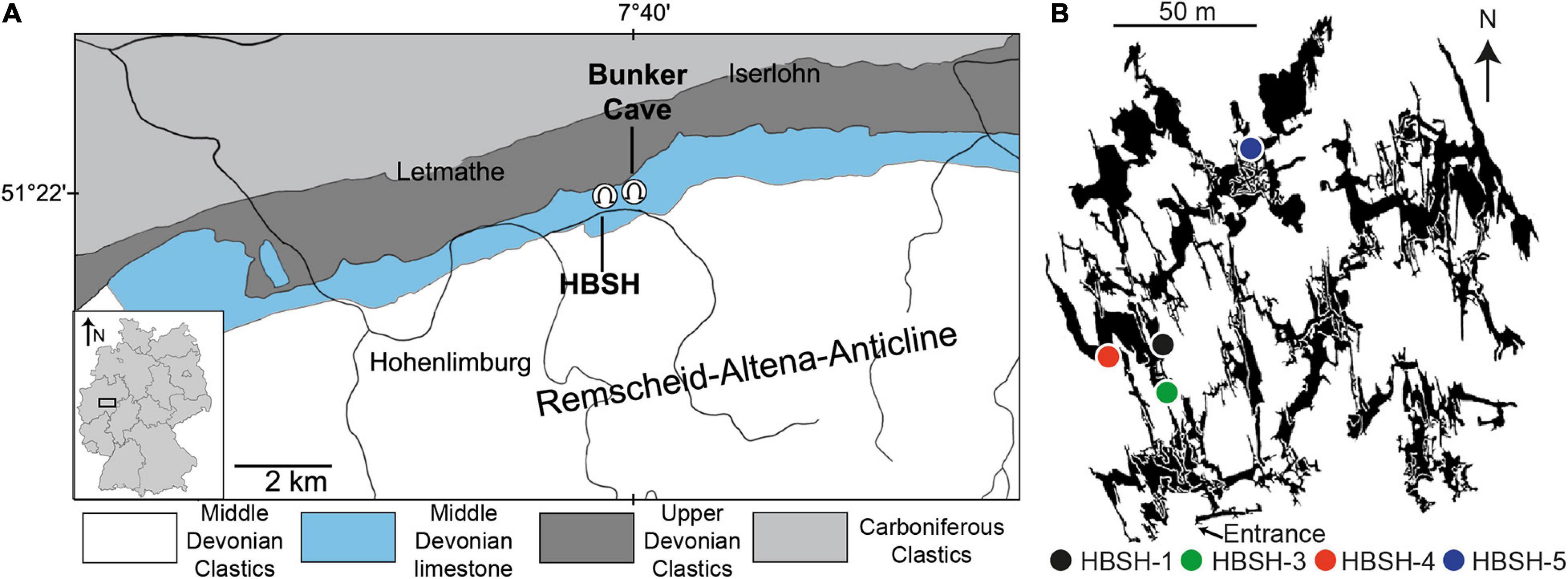
Figure 1. (A) Geological map of the cave area with the locations of Hüttenbläserschachthöhle (HBSH) and Bunker Cave. Modified after Riechelmann et al. (2011). (B) Cave map of HBSH with the location of the stalagmite sampling sites. Modified after Grebe (1994).

Hüttenbläserschachthöhle was discovered in 1993 and is one of the largest and speleothem-richest caves in Iserlohn-Letmathe (Hammerschmidt et al., 1995; Richter et al., 2015). The cave has a total length of 4.8 km with a vertical extent of 46 m (Grebe, 1994) and consists of three levels. On each level, a main corridor exists, which probably represents the former phreatic karst water collector. The cave levels can be correlated to river terraces in the Rhenish Slate Mountains (Niggemann et al., 2003). The area above HBSH and the nearby Bunker Cave is covered by similar vegetation consisting of C3-plants such as ash, beech trees and shrubs. The mean annual precipitation is 972 ± 173 mm (1 SD, 1978–2020) and the mean annual temperature in the area is 8.9 ± 0.7°C (1 SD; 1994–2020, DWD weather station Lüdenscheid, approximately 15 km south of HBSH). The δ¹⁸O values of precipitation range from −5‰ in summer to −13‰ in winter and averages −8.0 ‰ between 2006 and 2013 (Riechelmann et al., 2017).

Speleothem Samples

The four stalagmites covering the Holocene (HSBH-1, HBSH-3, HBSH-4, and HBSH-5, Figure 2) were collected from deep parts of HBSH. HBSH-1 is a ca. 55 cm-long stalagmite with clearly visible macroscopic banding. X-ray diffraction revealed that most of the sample consist of aragonite, with very few and short calcite sections (Jochum et al., 2012; Yang et al., 2015; Lin et al., 2017). This study focuses on an approximately 5 cm-long section from the top of the stalagmite. In contrast to HBSH-1, all other stalagmites of this study consist of calcite. HBSH-3 is approximately 22 cm long, banded and bright beige colored with some interspersed darker areas. HBSH-4 also shows banding throughout the whole stalagmite, which measures 30 cm in length, with a bright beige to gray colur. HBSH-5 has a total length of 33 cm, showing macroscopic banding and a generally darker color than the other HBSH stalagmites. While stalagmites HBSH-1, -3, and -4 grew in close proximity in the western part of HBSH, HBSH-5 was sampled in the norther part of HBSH (Figure 1B). This area is only sparsely decorated with speleothem deposits, potentially related to limited fractures in the overlying host rock (Hammerschmidt et al., 1995). The top section of HBSH-5 covering approximately 6 cm was investigated in this study.

FIGURE 2

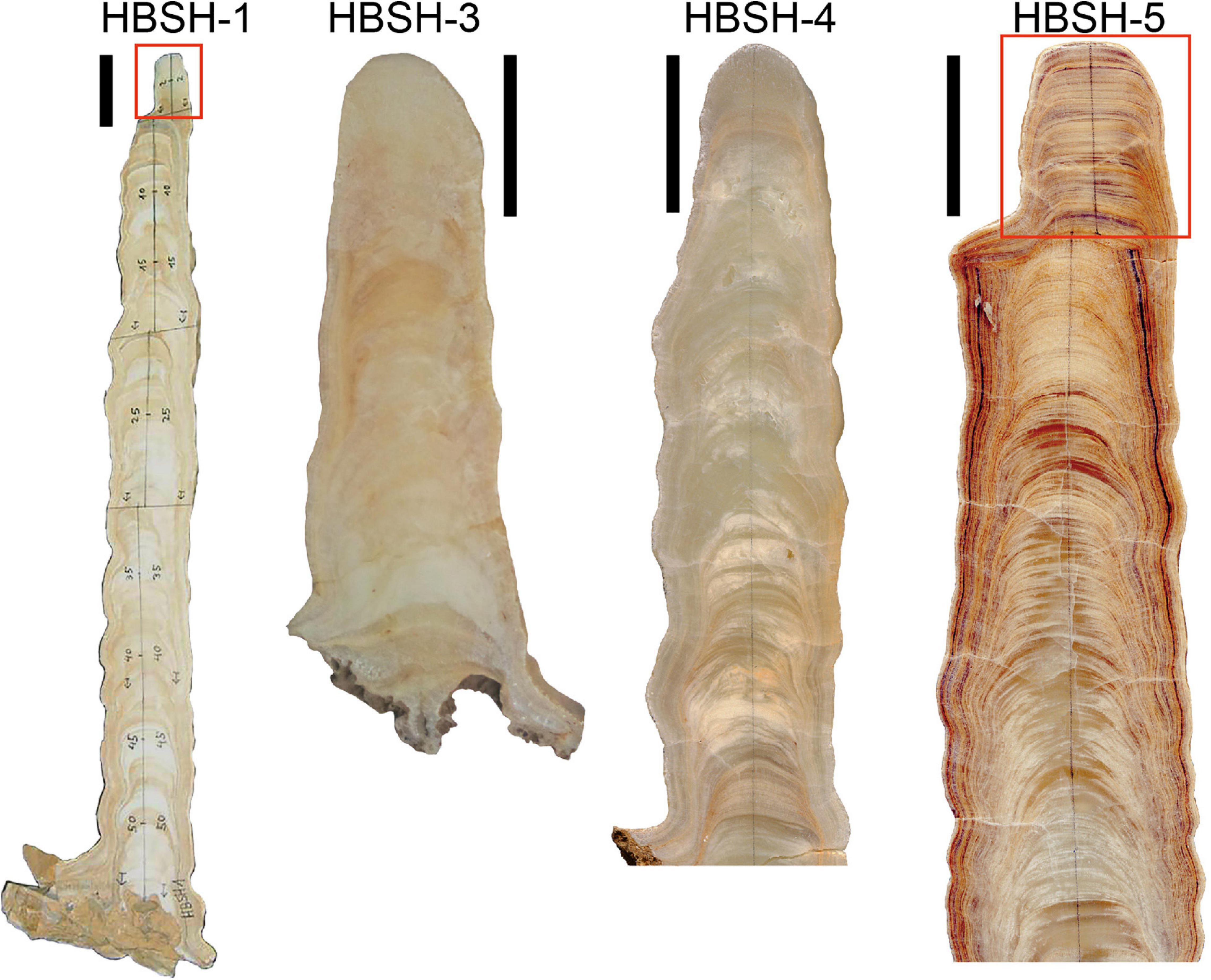
Figure 2. Pictures of the HBSH stalagmites. For HBSH-1 and HBSH-5, only the upper parts covering the Holocene (highlighted by the red box) were investigated. For HBSH-3 and HBSH-4, the major parts grew during the Holocene. All scale bars are 5 cm.

Analytical Methods

²³⁰Th/U-Dating

Stalagmite samples were dated using the ²³⁰Th/U dating method and analyzed by multi-collector inductively coupled plasma mass spectrometry (MC-ICP-MS) at the Max Planck Institute for Chemistry (MPIC), Mainz, the Institute for Geosciences, Mainz, and the Bristol Isotope Group (BIG), Bristol (HBSH-1). Samples were cut along the growth axes using a diamond wire saw. In total, 47 samples were analyzed at MPIC, seven samples at the Institute for Geosciences, Mainz, and five samples at BIG (Table 1). For sample HBSH-3, HBSH-4, and HBSH-5, sample amounts of approximately 300 mg were used, and chemical separation of U and Th prior to analysis was performed at the MPIC and the Institute for Geosciences following the methods described in Hoffmann (2008) and Yang et al. (2015). Chemical separation for HBSH-1 was performed at BIG as described by Hoffmann et al. (2007). At MPIC, a Nu Plasma MC-ICP-MS was used to analyze U and Th in separated sessions following the protocol described in Obert et al. (2016). Details of the calibration of the U-Th-spike are presented by Gibert et al. (2016). Introduction of the samples dissolved in 0.8 mol/L HNO₃ was performed using a CETAC Aridus II desolvating nebulizer system. A daily tuning protocol was used to achieve highest signal intensities and optimized peak shapes. At the Institute for Geosciences, a Neptune Plus MC-ICP-MS was coupled to a CETAC Aridus 3 desolvating nebulizer system, performing the same protocol as described for the Nu Plasma at MPIC. Measurements at BIG were performed using a Neptune MC-ICP-MS coupled to a CETAC Aridus desolvating system, following the methods described in Hoffmann et al. (2007). Age-depth models (Figure 3) were calculated using the algorithm StalAge (Scholz and Hoffmann, 2011).

TABLE 1

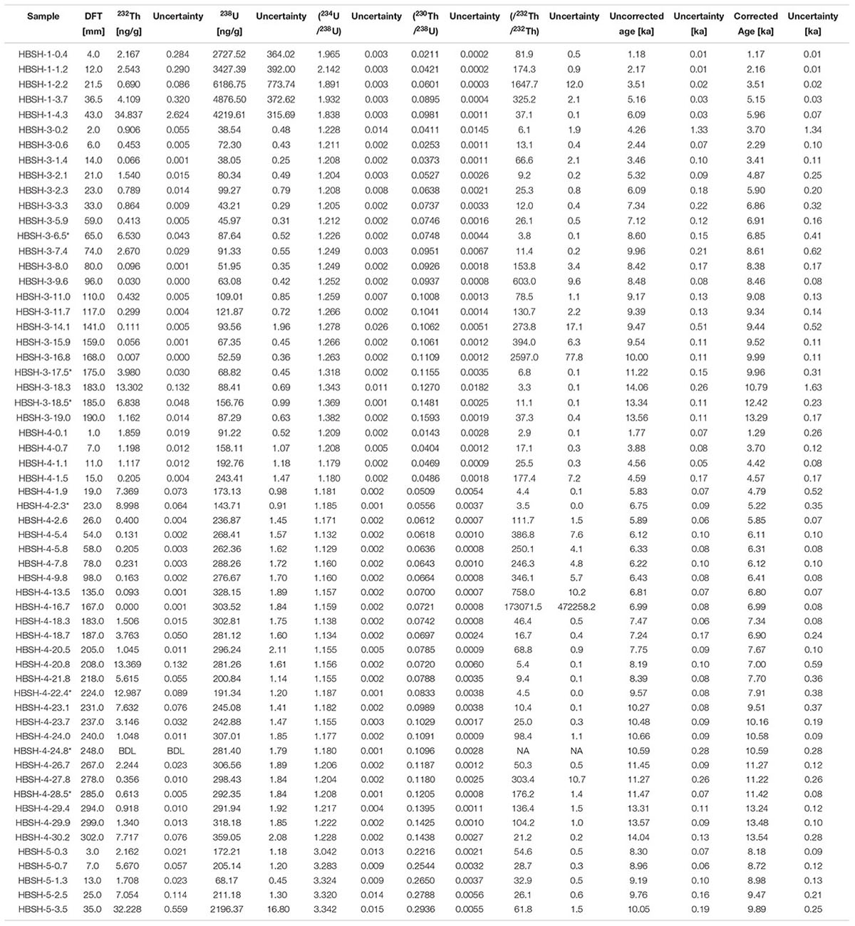
Table 1. Uranium and Th concentrations, activity ratios and ²³⁰Th/U-ages for the Holocene stalagmites from HBSH. All uncertainties are quoted as 2 SE. All activity ratios and ages were corrected for detrital contamination assuming a ²³²Th/²³⁸U mass ratio of 3.8 ± 1.9, calculated from the average Th and U concentrations of tonalities which are believed to be representative for the bulk continental crust (Wedepohl, 1995). ²³⁰Th, ²³⁴U, and ²³⁸U were assumed to be in secular equilibrium for the detritus. Activity ratios were calculated using the half-lives from Cheng et al. (2000). All measurements highlighted with an asterisk were measured at the Institute for Geosciences with a Neptune Plus MC-ICP-MS. Sample HBSH-1 was analyzed at the BIG. BDL = below detection limit; NA = not available due to ²³²Th concentration below detection limit. All ages are given relative to the year AD 2000.

FIGURE 3

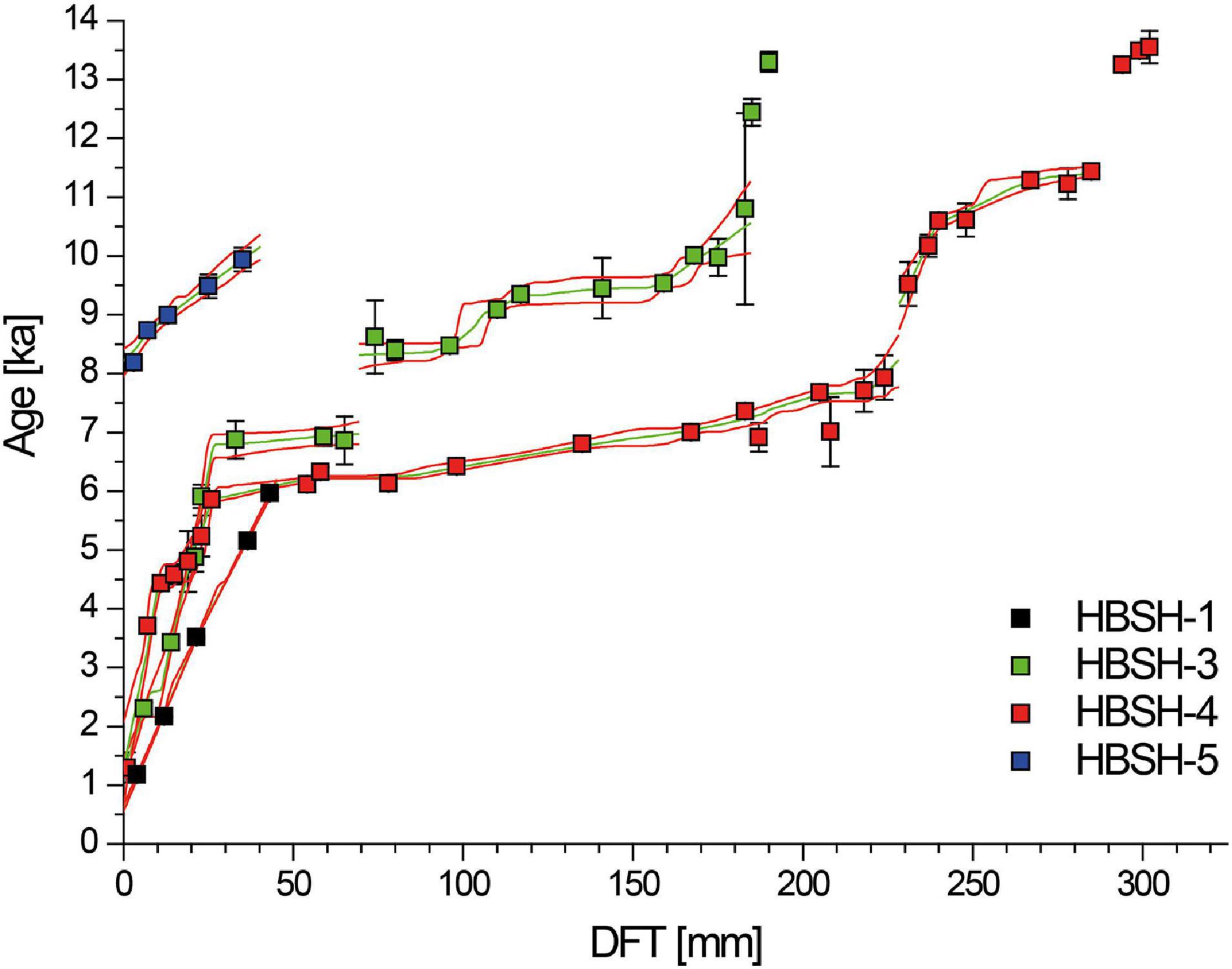
Figure 3. Age-depth relationships for stalagmites HBSH-1 (black), HBSH-3 (green), HBSH-4 (red), and HBSH-5 (blue). The colored squares represent the individual ²³⁰Th/U-ages with their respective 2 SE uncertainties. Note that some of the error bars are smaller than the symbols. Detailed uncertainties are given in Table 1. The green lines represent the age models calculated by StalAge (Scholz and Hoffmann, 2011) with the red lines representing the corresponding age uncertainties at the 95% confidence level for each sample. For the sections corresponding to the periods prior to the onset of the Holocene in stalagmites HBSH-3 and HBSH-4, no age model was calculated.

Stable Isotope Analysis

Stable carbon and oxygen isotope values (δ¹³C and δ¹⁸O) for HBSH-3, HBSH-4, and HBSH-5 were determined at the Institute for Geosciences, Johannes Gutenberg University Mainz. Samples were obtained with a semi-automated drilling device at a spatial resolution of 500 μm. In total, 1350 samples were analyzed using a Thermo Fisher Scientific MAT 253 continuous-flow isotope ratio mass spectrometer equipped with a Gasbench II. Stable carbon and oxygen isotope values for HBSH-1 were obtained at the Institute of Geology, University of Innsbruck, using a Merchantek video-controlled Micromill device (Dettman and Lohmann, 1995) at a spatial resolution of 150 μm, resulting in a total number of 301 samples. Analyses were performed using a Thermo Fisher Scientific Delta^plusXL isotope ratio mass spectrometer linked to a Gasbench II. Analytical precision and accuracy at the 1 σ-level was better than 0.08 ‰ for δ¹³C and δ¹⁸O. All values are reported relative to V-PDB.

Trace Element Analyses

Laser ablation inductively coupled plasma mass spectrometry (LA-ICP-MS) was used to determine trace element concentrations in HBSH-1, HBSH-3, and HBSH-5. A Thermo Fisher Scientific Element 2 SF-ICP-MS was coupled to a New Wave UP-213 laser ablation system at the MPIC. For all samples, the following laser parameters were applied: spot analyses with a spot size of 100 μm, a repetition rate of 10 Hz and an energy output of 60%, resulting in a fluence of ≈5 J/cm². Background signals were collected for 14 s prior to ablation and subtracted from the sample signal, followed by a wash-out time of 20 s. The following analytes were measured during the session: ²⁵Mg, ³¹P, ⁸⁸Sr, and ¹³⁷Ba. NIST SRM 612 was analyzed for calibration purposes at the beginning, between each set and at the end of the routine. ⁴³Calcium was used as internal reference to calculate trace element concentrations. Data evaluation was performed offline, following the calculations presented in Mischel et al. (2017b).

Data Processing and Statistics

All speleothems show a high variability in growth rate, both within individual stalagmites and between coeval stalagmites (Figure 4 and Supplementary Figure A4). Therefore, the stable isotope and trace element data shows high variability in temporal resolution. The aim of this study is to identify common long-term trends in the proxy records of the different samples, independent of the absolute δ¹³C and δ¹⁸O values, as well as trace element concentrations. To overcome potential biases due to differences in age resolution, centennial means for the stable isotope and trace element data were calculated. This is also a basic requirement for regression analysis (see sections “Within-cave correlation of speleothem records from HBSH and Bunker Cave” and “Inter-cave correlation of speleothem records from HBSH and Bunker Cave”), which was performed with the centennial stable isotope data using the statistical software R (R Core Team, 2020). The stalagmite samples differ in their mineralogy (i.e., aragonite and calcite) as well as growth rate and absolute δ¹³C and δ¹⁸O values. These differences can cause steps in the stacked isotope time series, which is particularly important for intervals of low replication, and if only a single stalagmite is available for a specific time interval. To avoid steps in the final dataset (Figures 4, 5), a composite stack for HBSH (Figure 5) was constructed using scaled stable isotope data of each speleothem. Scaling was performed using the “scale()” function of the statistical software R (R Core Team, 2020) and refers to subtraction of the mean and division by the standard deviation for each time series. Due to the scaling, differences in absolute δ¹³C and δ¹⁸O values can be neglected. After calculating the scaled stable isotope data for each stalagmite, a composite stack was constructed using the previously calculated centennial means of all HBSH stalagmites. The number of individual analyses, which were arithmetically averaged for each mean value (replication), are also provided. These calculations were not only performed for HBSH, but also for the stable isotope values from stalagmites from Bunker Cave covering the same time interval (Fohlmeister et al., 2012). Principal component analysis (PCA) was performed with the centennial means for stable isotope and trace elements and the “fviz_pca_biplot()” function of the statistical software R (R Core Team, 2020) and centennial means were calculated for stable isotopes and trace elements. To test the suitability of our dataset for PCAs and justify this approach, the Kaiser-Meyer-Olkin test for sampling adequacy (>0.5; Kaiser, 1970; Kaiser and Rice, 1974) and Bartlett’s test of sphericity (<0.05; Bartlett, 1937) were employed. Sample HBSH-5 did not pass the Kaiser-Meyer-Olkin test. Only principal components (PCs) with a standard deviation > 1.0 were considered and a cut-off value of 0.4 was chosen to describe the most important parameters of the PCA (Budaev, 2010). Detailed results including eigenvalues and factor loadings are presented in Supplementary Table A1. To evaluate the relationship between trace element and stable isotope data, a correlation analysis was performed using the statistical software R (R Core Team, 2020).

FIGURE 4

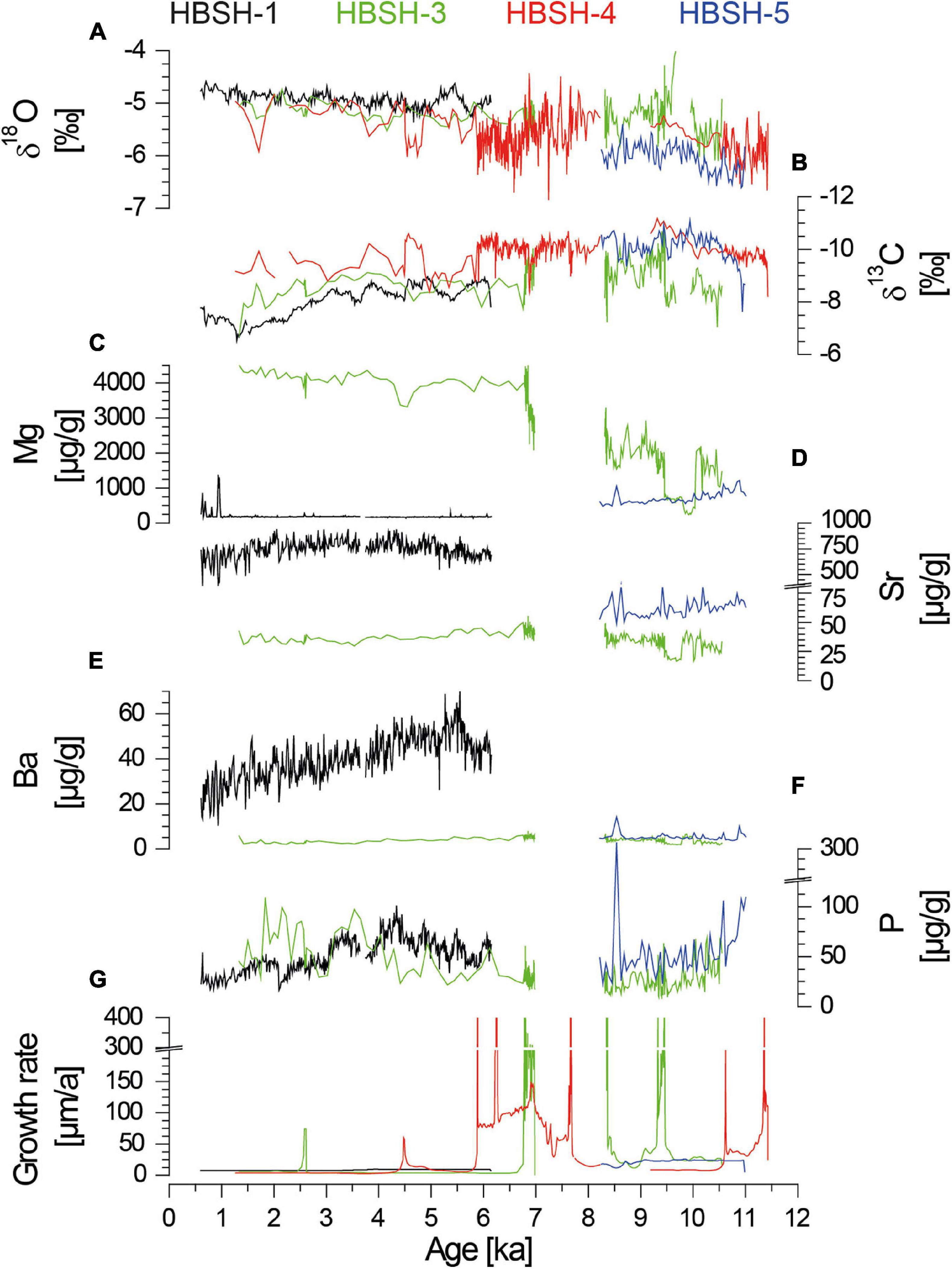
Figure 4. Proxy data for stalagmites HBSH-1 (black), HBSH-3 (green), HBSH-4 (red) and HBSH-5 (blue) based on the age-depth model. (A) δ¹⁸O and (B) δ¹³C values. (C) Mg, (D) Sr, (E) Ba, and (F) P concentrations. (G) Growth rate. Note the inverted axis for δ¹³C and the breaks in the y-axis for Sr, P, and growth rate.

FIGURE 5

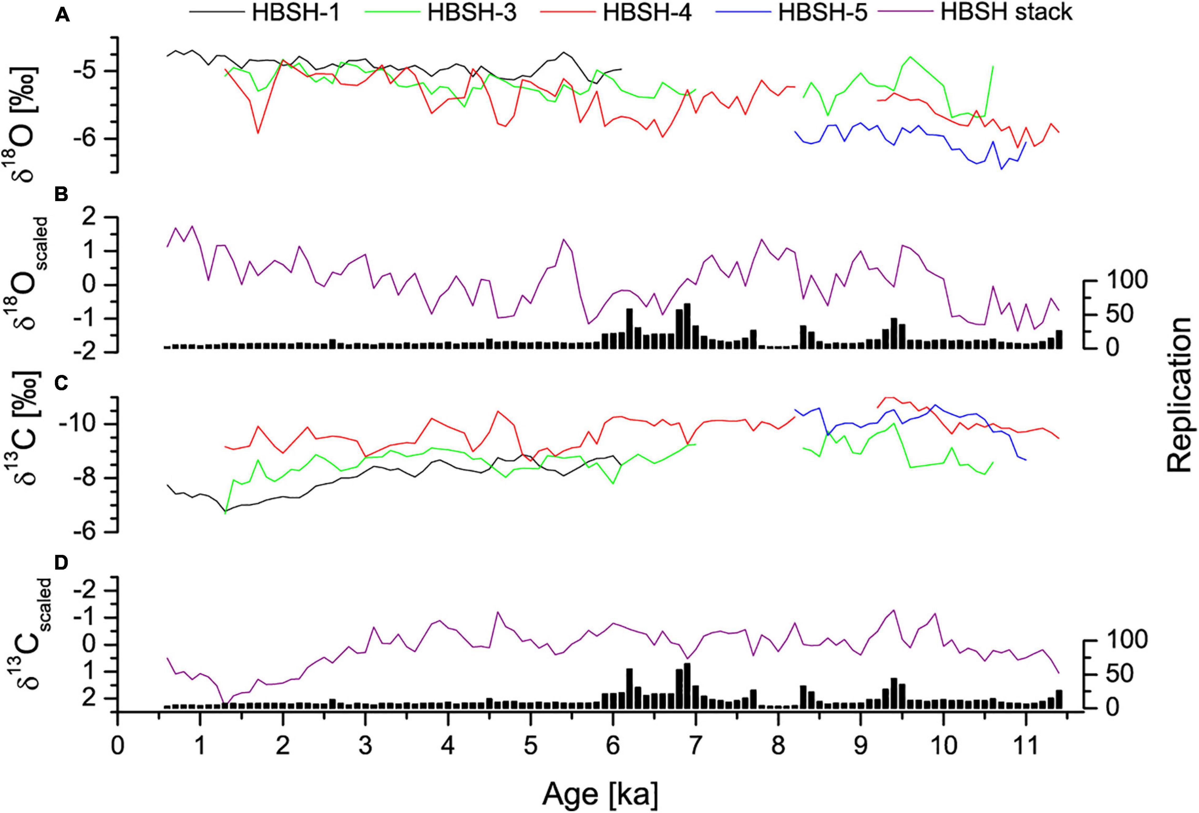
Figure 5. (A) δ¹⁸O and (C) δ¹³C values averaged by a centennial mean for stalagmites HBSH-1 (black), HBSH-3 (green), HBSH-4 (red), and HBSH-5 (blue). Scaled stable isotope time series for δ¹⁸O values (B) and δ¹³C values (D). For all records, the replication indicates the number of stable isotope measurements averaged for the centennial mean for the specific time interval. Note the inverted axis for δ¹³C.

Strontium Isotope Analyses

Strontium isotope ratios (⁸⁷Sr/⁸⁶Sr) were determined for speleothem samples HBSH-3 (n = 9), HBSH-4 (n = 9), and HBSH-5 (n = 3). The samples (2 – 7 mg) were processed at the Institute for Geosciences, using a laminar flow hood in a clean laboratory, following the methods described by Lugli et al. (2017) and Weber et al. (2018b) for dissolution and separation of Sr using Sr-spec resin. ⁸⁷Sr/⁸⁶Sr ratios were determined at the MPIC using a Nu Plasma MC-ICP-MS coupled to a CETAC Aridus II desolvating nebulizing system following the methods described by Weber et al. (2017). Ion beams were simultaneously collected using seven Faraday cups covering the m/z range of 82 – 88, representing the following isotopes: ⁸²Kr, ⁸³Kr, ⁸⁴Sr, ⁸⁵Rb, ⁸⁶Sr, ⁸⁷Sr, and ⁸⁸Sr. Strontium solutions were diluted to approximately 50 μg/mL and measured in a standard-bracketing sequence, correcting for a NIST SRM 987 ⁸⁷Sr/⁸⁶Sr ratio of 0.710248 (McArthur et al., 2001). Correction for instrumental mass bias was performed using an exponential law, using a ⁸⁸Sr/⁸⁶Sr ratio of 8.375209 (Steiger and Jäger, 1977).

Results

²³⁰Th/U-Dating

Results of the ²³⁰Th/U-dating are presented in Table 1. Resulting age-depth models of all speleothem samples are presented in Figure 3, and all following ages refer to the age models resulting from StalAge (Scholz and Hoffmann, 2011). The studied section of speleothem HBSH-1 shows slow continuous growth between 6.1 ± 0.6 ka and 0.60 ± 0.06 ka with a stable growth rate of 8 μm/a (calculated based on the age-depth model). Sample HBSH-3 shows a more complex growth history. Two measurements yielded ages of 13.3 ± 0.2 ka and 12.4 ± 0.2 ka corresponding to the Bølling-Allerød. These ages were not included in the age model. Growth during the Holocene started at 10.8 ± 1.6 ka and continued at least until 8.3 ± 0.2 ka with the fastest growth rate (>100 μm/a) between 9.5 and 9.0 ka. A growth stop between 8.3 ± 0.2 ka and 7.0 ± 0.2 ka is indicated by the age-depth model and is followed by a phase of slow growth (6 μm/a) until the final stop at 1.3 ± 0.2 ka. The growth history of speleothem HBSH-4 is similar to HBSH-3 with an initial growth phase during the Bølling-Allerød between 13.6 ± 0.3 ka and 13.2 ± 0.1 ka, followed by a growth stop until 11.4 ± 0.1 ka, representing a growth inception shortly after the onset of the Holocene at 11.7 ± 0.1 ka. The initial growth phase for HBSH-4 lasted until 9.2 ± 0.4 ka and shows a deceleration from >30 μm/a to <10 μm/a toward a hiatus. Growth resumed around 8.2 ± 0.4 ka, and fast continuous growth (60 – 100 μm/a) is observed until 5.8 ± 0.1 ka, where a distinct growth deceleration (<10 μm/a) occurred, lasting until at least 3.7 ± 0.1 ka. The youngest age obtained from HBSH-4 is 1.3 ± 0.3 ka, and a continuous growth of approximately 3 μm/a until then is assumed. Speleothem HBSH-5 shows continuous growth between 9.9 ± 0.3 ka and 8.2 ± 0.1 ka and a rather constant growth rate of ≈20 μm/a for most of the studied part of the specimen. Only the youngest part shows a decelerating growth rate down to ≈10 μm/a between 8.7 ± 0.1 ka and 8.2 ± 0.1 ka.

Trace Elements

Trace element records of HBSH-1, -3, and -5 of Mg, P, Sr and Ba are presented in Figure 4 and Supplementary Figures A1–A3.

Since HBSH-1 consists of aragonite (in contrast to the calcite speleothems HBSH-3 and HBSH-5), its trace element concentrations differ significantly from those of the other stalagmites (c.p., Wassenburg et al., 2016b). Magnesium in HBSH-1 is low (≈180 μg/g) for major parts of the sample except for some spikes, during the most recent 1000 years. For the whole growth phase, no general increasing or decreasing trend in Mg is visible. The Sr concentration is relatively high in comparison to the calcite speleothems, increasing from 500 to 800 μg/g towards more recent ages until 3.5 ± 0.1 ka. Afterward, this trend is reversed. The same pattern is visible in P, while Ba decreases on a longer time scale toward younger ages.

HBSH-3 has a much higher Mg concentration (1000 and 4500 μg/g). In general, Mg increases toward younger ages, especially in the second growth phase between 7.0 ± 0.2 ka and 1.3 ± 0.2 ka. Strontium and Ba show a similar trend with increasing concentrations until the growth stop and decreasing concentrations after growth resumed at 7.0 ± 0.2 ka. The opposite trend is true for P. A prominent feature is the decrease in concentration for Mg, Sr and Ba around 9.5 ± 0.2 ka.

HBSH-5 does not show large trace element variations besides an increase in Mg, Ba, and P around 8.5 ± 0.2 ka, which is contemporaneous with a decrease in Sr concentration. In general, all four observed trace element concentrations decrease toward the growth stop around 8.2 ± 0.1 ka.

Stable Isotopes

The δ¹³C values are presented in Figure 4B. Since the four speleothems show different growth rates, a centennial mean based on the age-depth model for each speleothem sample (Figure 5C) was calculated to focus on longer-term trends. Stalagmites HBSH-3 and HBSH-4 started to grow at the beginning of the Holocene, or shortly after, while growth of HBSH-5 re-initiated at that time. The three stalagmites start with similar δ¹³C values (between −8 and −9 ‰) and then rapidly tend toward more negative values until reaching their most negative values around 9.5 ka. HBSH-3 and HBSH-4 also reached their most negative δ¹³C values almost simultaneously around 9.4 ± 0.1 ka, when HBSH-5 also shows a negative peak in δ¹³C. Shortly afterward, HBSH-4 stopped growing, while HBSH-3 and HBSH-5 continued to grow until 8.3 ± 0.2 ka and 8.2 ± 0.1 ka, respectively, and show again less negative δ¹³C values. HBSH-4 started growing again around 8.2 ± 0.4 ka with δ¹³C values fluctuating between −10 and −9‰ with two negative peaks around 4.6 ± 0.2 ka and 3.8 (+0.6, −0.2) ka. HBSH-3 started to grow again at 7.0 ± 0.2 ka with a trend toward less negative δ¹³C values, which was further intensified after 3.0 ± 0.3 ka, reaching a peak δ¹³C value of −6.7‰ at 1.3 ± 0.2 ka, coherent with the final growth stop. The Holocene growth phase of the aragonitic speleothem HBSH-1 commenced at 6.1 ± 0.6 ka with an initial decrease in δ¹³C values, followed by a long-term trend toward more negative values, similar to HBSH-3. Negative δ¹³C peaks occur in HBSH-1 at 6.0 ± 0.1 ka, 4.6 ± 0.1 ka and 3.9 ± 0.1 ka, all coherent with peaks in δ¹³C values in HBSH-4. When HBSH-1 reached its most positive δ¹³C value of −6.5 ‰ at 1.3 ± 0.2 ka, HBSH-3 and HBSH-4 stopped growing, while HBSH-1 continued to grow with decreasing δ¹³C values until the final growth stop at 0.6 ± 0.1 ka.

Oxygen isotope results of all the HBSH speleothems show a general trend toward less negative δ¹⁸O values during the Holocene. As the δ¹³C values, the δ¹⁸O values (Figure 4A) show more variable values on annual to decadal time scales. To focus on the long-term trends, centennial means of the δ¹⁸O values (Figure 5A) were computed. In contrast to the δ¹³C values, the δ¹⁸O values show a more coherent trend in all speleothems. After an initial decrease shortly after growth inception in HBSH-3, HBSH-4 and HBSH-5, these three speleothems show a trend toward less negative δ¹⁸O values until their growth stops at 9.2 ± 0.4 ka (HBSH-4), 8.3 ± 0.2 ka (HBSH-3) and 8.2 ± 0.1 ka (HBSH-5). The least negative δ¹⁸O value of all speleothems is observed in HBSH-3 around 9.6 ± 0.1 ka (−4.6 ‰) and is in agreement with less negative values in HBSH-4 and HBSH-5. Subsequent to the growth stops in HBSH-3 and HBSH-4, both speleothem samples show less negative δ¹⁸O values, although HBSH-4 shows a decrease between 6.7 ± 0.3 ka and 5.8 ± 0.4 ka. Growth in the Holocene part of HBSH-1 started at 6.1 ± 0.6 ka and also tends to less negative δ¹⁸O values throughout the Holocene. The most prominent positive peak in δ¹⁸O values in HBSH-1 occurred around 5.4 ± 0.1 ka. HBSH-4 shows a coherent increase in δ¹⁸O values during that time. HBSH-1 does not show any further prominent δ¹⁸O peaks until its growth stopped around 0.6 ± 0.1 ka. However, HBSH-3 and HBSH-4 show a further trend toward less negative δ¹⁸O values around 1.7 ± 0.5 ka, which is not reflected in HBSH-1.

Strontium Isotopes

HBSH-5 shows the least radiogenic ⁸⁷Sr/⁸⁶Sr ratios of 0.70899 ± 0.00002 at 9.8 ± 0.2 ka and 0.70882 ± 0.00002 at 8.8 ± 0.1 ka, followed by a strongly decreasing trend toward modern time (Figure 6). HBSH-4 shows the same trend in the older growth section toward lower Sr isotope ratios. However, the ⁸⁷Sr/⁸⁶Sr ratios of HBSH-4 are overall higher with values between 0.70950 ± 0.00002 and 0.70977 ± 0.00002. The lowest value of 0.70950 ± 0.00002 is observed at 6.5 ± 0.1 ka, followed by an increase toward 0.70966 ± 0.00002 at 6.0 ± 0.1 ka. Toward the final growth stop of HBSH-4 at 1.3 ± 0.2 ka, the ⁸⁷Sr/⁸⁶Sr ratio becomes progressively higher. HBSH-3 shows the highest Sr isotope ratios, with all ⁸⁷Sr/⁸⁶Sr values above 0.70987 ± 0.00002. While the first growth phase shows identical ⁸⁷Sr/⁸⁶Sr within uncertainties (0.71009 ± 0.00002 and 0.71008 ± 0.00002), the second growth phase shows the lowest ⁸⁷Sr/⁸⁶Sr of 0.70987 ± 0.00002 at 7.0 ± 0.2 ka. Afterward, the values increase toward 0.71003 ± 0.00002 at 6.8 ± 0.2 ka and progressively become higher toward younger ages with a maximum ⁸⁷Sr/⁸⁶Sr ratio of 0.71016 ± 0.00002 at 2.2 ± 0.2 ka.

FIGURE 6

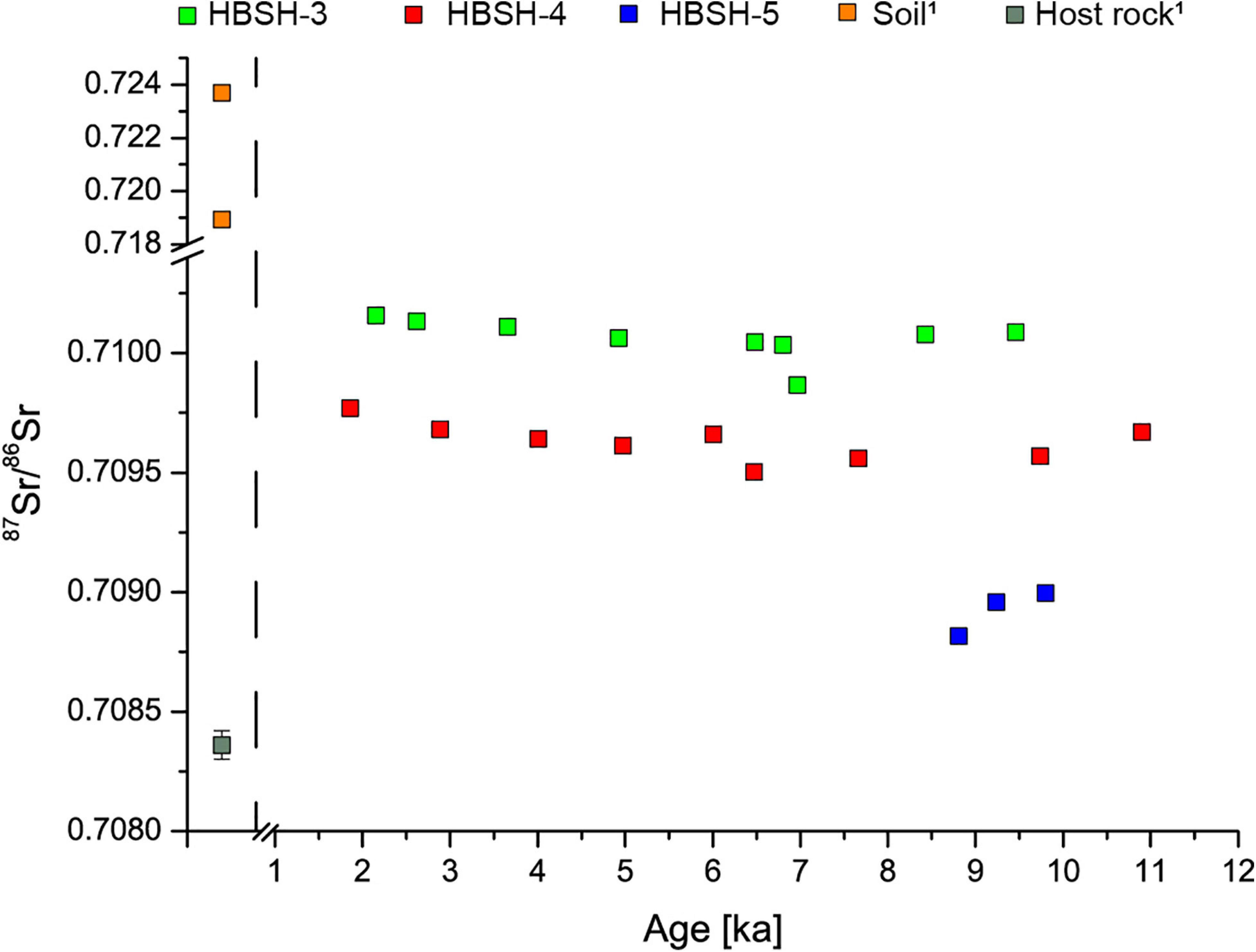
Figure 6. Strontium isotope results for HBSH-3 (green), HBSH-4 (red), and HBSH-5 (blue). ¹Sr isotope values from the host rock and overlying soil at the nearby Bunker Cave (Weber et al., 2018a). Note that analytical uncertainties are usually smaller than the plot symbols.

Discussion

Growth Phases

The four HBSH speleothem samples cover almost the entire Holocene, except the most recent 600 years. Earlier growth phases were identified between 13.6 ± 0.3 ka and 13.3 ± 0.1 ka for HBSH-4 and between 13.3 ± 0.2 ka and 12.4 ± 0.2 ka for HBSH-3 (Table 1). These initial growth phases correspond to the Bølling-Allerød interstadial (Köhler et al., 2011).

Based on the age-depth model of HBSH-4, growth during the Holocene commenced at 11.4 ± 0.1 ka. Growth of HBSH-5 re-initiated shortly afterward at 11.0 ± 0.4 ka. Based on the age model, a simultaneous growth start is possible, but this cannot be resolved. The onset of growth in HBSH-3 occurred around 10.6 ± 0.6 ka, which is shortly after HBSH-4 and HBSH-5. Therefore, it is presumed that the climate amelioration at the onset of the Holocene triggered speleothem growth in HBSH between about 11.4 and 10.6 ka. Between 10.6 and 9.2 ka, the three speleothems grew simultaneously until HBSH-4 stopped at 9.2 ± 0.4 ka. Interestingly, when growth of HBSH-3 and HBSH-5 had stopped (8.3 ± 0.2 ka), HBSH-4 started to grow again at 8.2 ± 0.4 ka with a growth rate rapidly increasing from <10 μm/a to up to >100 μm/a (Figure 4G and Supplementary Figure A4). HBSH-4 growth rate declined after 6.0 ± 0.1 ka to <10 μm/a. The growth rate of HBSH-3 declined around 6.5 ± 0.4 ka with values <10 μm/a in the same range as observed for HBSH-4 (Figure 4G and Supplementary Figure A4). Growth of HBSH-1 between 6.1 ± 0.6 ka and 0.6 ± 0.1 ka was continuous for the whole growth period, but the growth rate was very small (< 10 μm/a) and agrees with the rates observed in HBSH-3 and HBSH-4, although those are more variable (Figure 4G and Supplementary Figure A4). In general, the older growth phase during the first half of the Holocene was characterized by higher growth rates than the younger phase. The transition between these two phases in HBSH occurred between 7 and 6 ka and was marked by a reduction in growth rate. This is evident from all four speleothems from HBSH: the two speleothems covering this transition (HBSH-3 and HBSH-4) as well as the two stalagmites that only grew during one of these phases (HBSH-5 in the older phase and HBSH-1 in the younger phase).

Stable Isotopes

The δ¹⁸O values of all Holocene HBSH speleothems show the same increasing trend on the long time-scale (Figures 4A, 5A). At the onset of the Holocene, δ¹⁸O values are lowest in the three coeval specimens HBSH-3, HBSH-4, and HBSH-5, although their absolute values differ. A first peak in δ¹⁸O values is reached around 9.4 ka, with maximum values in HBSH-3 and HBSH-4. HBSH-5 reached a stable value of ca. −5.5 ‰ at that time and remained at that level until the final growth stop at 8.2 ± 0.1 ka. In HBSH-3, the δ¹⁸O values slightly decrease until the growth stop at 8.3 ± 0.2 ka. Simultaneously, HBSH-4 started to grow again with less negative values than prior to the growth stop and remained at that level (ca. −5 ‰) until 7.0 ± 0.1 ka. At that time, δ¹⁸O values decrease by around 1‰ and HBSH-3 started to grow again. From that on, the δ¹⁸O values increase progressively until growth finally stopped. When HBSH-1 started to grow at 6.1 ± 0.6 ka, the δ¹⁸O values also progressively increased until the least negative δ¹⁸O value of −4.7 ‰ at 0.6 ± 0.1 ka. After 5 ka, the three coeval speleothems show comparable δ¹⁸O values.

For speleothem δ¹⁸O values, the major influencing factors are the cave temperature and the δ¹⁸O value of precipitation above the cave. The δ¹⁸O value of modern precipitation in the cave region varies between −5 ‰ in summer and −13 ‰ in winter, resulting in an infiltration-weighted δ¹⁸O value of −8.1 ‰ (Riechelmann et al., 2017). In comparison to the nearby Bunker Cave, the δ¹⁸O values in the younger parts of the HBSH samples are less negative. Recent calcite precipitates from Bunker Cave show a relationship between δ¹⁸O values and drip rate. The calcite δ¹⁸O values for a fast-dripping site are −6.3 ± 0.3 ‰ and −5.6 ± 0.2 ‰ for a slow dripping site (Riechelmann et al., 2013). Hence, it is reasonable to assume that the high δ¹⁸O values of the HBSH stalagmites indicate very slow drip rates. However, considering that the δ¹⁸O values of the HBSH stalagmites are generally higher than those of the Bunker Cave stalagmites, they were probably also influenced by additional factors. In Bunker Cave, Holocene δ¹⁸O variability has been mainly attributed to changes in winter precipitation and temperature (Fohlmeister et al., 2012). In that study, less negative speleothem δ¹⁸O values were interpreted to reflect cold and dry winters and vice versa. In HBSH, this interpretation would indicate a trend toward colder and dryer winters during the course of the Holocene. Besides climatic factors, disequilibrium isotope fractionation can influence the δ¹⁸O values of speleothems (Lachniet, 2009; Mühlinghaus et al., 2009; Deininger et al., 2012; Hansen et al., 2019). Since a trend toward slower growth rates with time in the HBSH speleothems is observed, these disequilibrium effects may have altered the δ¹⁸O values due to increasing drip intervals (Hendy, 1971; Lachniet, 2009; Riechelmann et al., 2013; Dreybrodt et al., 2016; Hansen et al., 2019), causing δ¹⁸O values to increase. In addition, prior calcite precipitation (PCP) is another factor potentially influencing the stable isotope signals.

The HBSH speleothems show generally different δ¹³C values during the first and the second part of the Holocene, starting around 7 – 6 ka (Figures 4B, 5C). After growth inception, the δ¹³C values tend toward more negative values in HBSH-4 and HBSH-5, which is most likely related to the climate amelioration at the onset of the Holocene. Increased biological activity and vegetation development in the newly formed soil results in more negative δ¹³C values, due to the biological fractionation of carbon in the soil with increased biological activity (McDermott, 2004). This trend is less clear for HBSH-3. However, this might be related to a later onset of growth of this speleothem, where the overlying soil and vegetation was already established. The most negative peak in δ¹³C is reached around 9.4 ka in HBSH-3 and HBSH-4, with HBSH-5 showing a negative peak as well. This is coherent with a maximum in δ¹⁸O of these three speleothems (Figures 4, 5). In general, this older phase seems to be characterized by increased soil biological activity and root respiration, indicating relatively warm and humid climate conditions during the early Holocene at HBSH. Interestingly, HBSH-4 stopped growing shortly after reaching its most negative δ¹³C values, while HBSH-5 remains at that δ¹³C level and HBSH-3 shows a slight trend toward less negative values until these stalagmites stopped to grow at 8.3 ± 0.2 ka and 8.2 ± 0.1 ka, respectively. At the same time, HBSH-4 resumed growth with δ¹³C values around −10 ‰ and the highest growth rate of the entire stalagmite. The negative δ¹³C values and the high growth rate suggest favorable climate conditions at that time, consistent with the Holocene climate optimum (Mayewski et al., 2004). HBSH-3 started to grow again at 7.0 ± 0.2 ka with a high growth rate and δ¹³C values around -9.5 ‰. However, growth rate in HBSH-3 rapidly declined after re-inception of growth and the δ¹³C values increase toward −8 to −8.5 ‰. This pattern is also visible in HBSH-4 around 6 ka, where the δ¹³C values increase by more than 1 ‰ and growth rate declined to less than 10 μm/a. This coherent pattern indicates reduced water availability in the karst system, which can either be related to a climatic deterioration or hydrological changes in the epikarst and the vadose zoneresulting in reduced water availability in the cave. Due to the observed time lag of approximately 1,000 years between the two samples, this can potentially be caused by delayed changes in the water circulation routes in the overlying karst aquifer. Shortly before the transition toward less negative δ¹³C values and slower growth rates in HBSH-4, stalagmite HBSH-1 recommenced growing at 6.1 ± 0.6 ka. The initial δ¹³C values changed rapidly toward more negative values, before reaching a minimum at 6.0 ± 0.1 ka. Further on, δ¹³C values of HBSH-1 progressively increased. The same trend is visible in HBSH-3, while the low growth rate of HBSH-4 resulted in smoothed signals. However, some coherent patterns can be identified. At 5 ka, HBSH-1 and HBSH-4 show a simultaneous decrease in δ¹³C until 4.5 ka, where δ¹³C values increase in both stalagmites. A second δ¹³C minimum is observed in all three speleothems at 4 ka. However, the general trend of δ¹³C values is still toward higher values, reaching their maximum at 1.3 ± 0.2 ka, when HBSH-3 and HBSH-4 finally stopped growing. In contrast, HBSH-1 continued to grow with a constant growth rate and decreasing δ¹³C values (−7.8 ‰ at 0.6 ± 0.1 ka).

Changes in δ¹³C values of speleothems have often been related to environmental and climatic factors, such as vegetation cover and soil biological activity. However, due to changes in the stalagmite growth rates, (disequilibrium) isotope fractionation during speleothem deposition may introduce substantial biases. For instance, an increase in δ¹³C values may not only reflect decreasing availability of soil CO₂, but also a decrease in drip rate, i.e., a longer residence time of the drip water on the speleothem surface, enhancing disequilibrium isotope fractionation (Mühlinghaus et al., 2009; Scholz et al., 2009; Deininger et al., 2012; Riechelmann et al., 2013). Since growth rate remarkably dropped in all speleothems around 7 – 6 ka, it is likely that the average drip interval in HBSH increased. This is a potential cause for the progressive increase in δ¹³C values of HBSH-1, HBSH-3, and HBSH-4 during the second half of the Holocene, because their growth rates are below <10 μm/a during that time interval. In contrast, the first part of the Holocene was characterized by a faster growth rate and decreasing δ¹³C values in HBSH. During this time interval, isotope disequilibrium effects on the speleothem surface played a minor role and the decreasing trend likely reflects increasing vegetation density, soil cover and biological activity.

Trace Elements

Trace elements in HBSH-5 show a decreasing trend toward the growth stop (Figure 4 and Supplementary Figure A3). At 8.5 ± 0.2 ka, Mg, P, and Ba increases, while Sr decreases. This timing is coherent with the negative peaks in δ¹³C and δ¹⁸O. In general, the correlation between the four investigated trace elements is positive, with Ba and P showing the highest correlation of R = 0.70 (Supplementary Figure A5, p < 4 × 10^–4). In addition, there is a positive correlation of R = 0.49 between δ¹³C and Mg (p < 7 × 10^–3), indicating PCP. Since the decrease in δ¹³C values is attributed to soil formation and increasing biological activity, the decrease in Mg seems to be also related to these processes, i.e., enhanced soil bioproductivity and wet conditions causing lower Mg concentrations (Riechelmann et al., 2012; Wassenburg et al., 2016b; Weber et al., 2018a). Furthermore, the decrease in Mg is similar as during the initial Holocene phase in Bunker Cave (Fohlmeister et al., 2012). The authors attributed this pattern to the deposition of Mg-bearing loess during the previous glacial period and the progressive leaching of carbonate from the loess in the early Holocene. Due to the close proximity (<1 km) to Bunker Cave, the same should be true for HBSH and is an additional explanation for the Mg trend observed in HBSH-5. Since HBSH-5 only covers the early part of the Holocene, the transition observed in the growth rate and stable isotopes is not captured by this speleothem. However, HBSH-3 covers most parts of the Holocene besides the hiatus between 8.3 ± 0.2 ka and 7.0 ± 0.2 ka. Therefore, changes between the two different phases in HBSH-3 are expected. The first growth phase of HBSH-3 shows lower Mg concentrations than the second one. This transition is visible in the results of the PCA (Figure 7B), where Mg separates the early (11.5 – 8.1 ka) and late (7.0 – 1.1 ka) growth phases along PC2. In addition, δ¹³C values are lower in the first growth phase. For the δ¹³C values, the PCA especially separates the growth phases between 9.3 – 8.1 ka and 4.0 – 1.1 ka along PC1. Based on the assumption proposed for HBSH-5, the first phase is expected to have been wetter and more strongly influenced by soil formation and biological activity. Due to the increase of Mg over time, the Mg concentration is positively correlated with the δ¹⁸O values (R = 0.51, p < 7 × 10^–3, Supplementary Figure A6). Similar or even higher correlations exist between Mg and Sr (R = 0.51, p < 6 × 10^–6) and Ba and Sr (R = 0.78, p < 2 × 10^–14), indicating the same source for Ba and Sr, most likely the host rock. However, the correlation between Sr and Mg is mainly based on the first growth phase, where Ba, Sr, and Mg increase. This is clearly visible in the correlation matrix in Figure 8A, where only data from the first growth phase (10.6 ± 0.6 to 8.3 ± 0.2 ka) are shown. Strontium and Ba show a strongly positive correlation (R = 0.92, p < 1 × 10^–16), as well as Sr and Mg (R = 0.72, p < 1 × 10^–16) and Ba and Mg (R = 0.53, p < 1 × 10^–16). Magnesium, however, is slightly negatively correlated with δ¹³C (R = −0.19, p < 0.04) and δ¹⁸O (R = −0.24, p < 0.005). In the second growth phase (7.0 ± 0.2 ka to 1.3 ± 0.2 ka), Mg further increases, while Ba and Sr decrease. The correlation matrix for the younger part (Figure 8B) shows, that Mg is positively correlated with both stable isotopes during this time span (δ¹³C R = 0.41, p < 5 × 10^–6, δ¹⁸O R = 0.23, p < 0.02). Furthermore, Mg is slightly negatively correlated with Ba (R = −0.39, p < 3 × 10^–6), while Sr and Ba still show a strong positive correlation (R = 0.92, p < 1 × 10^–16). This indicates an additional process during the younger part of the Holocene, which overprints the host rock signal for the trace elements and disrupts the relationship between Sr, Ba, and Mg, e.g., growth mechanisms of the speleothems (e.g., Paquette and Reeder, 1995; Fairchild et al., 2000; Treble et al., 2005; Mattey et al., 2010). The increase in Mg concentration may not only be attributed to changes in pathways in the vadose zone, but also to changes in the residence time of the percolating water. PCP (Fairchild et al., 2000; Riechelmann et al., 2011) can influence the Mg concentration, with increasing PCP leading to an increase in Mg in the speleothem (Tooth and Fairchild, 2003). This could explain increasing Mg concentrations in the younger part and supports the assumption of a drier climate. In addition, differences in dissolution characteristics of calcite and dolomite (Fairchild and Treble, 2009) can cause differences in the Mg concentration. The host rock of HBSH is similar to the host rock above Bunker Cave, where dolomite is present (Grebe, 1993). During drier conditions, the contribution of dolomite to the drip water will increase and result in increased Mg concentrations in the speleothems.

FIGURE 7

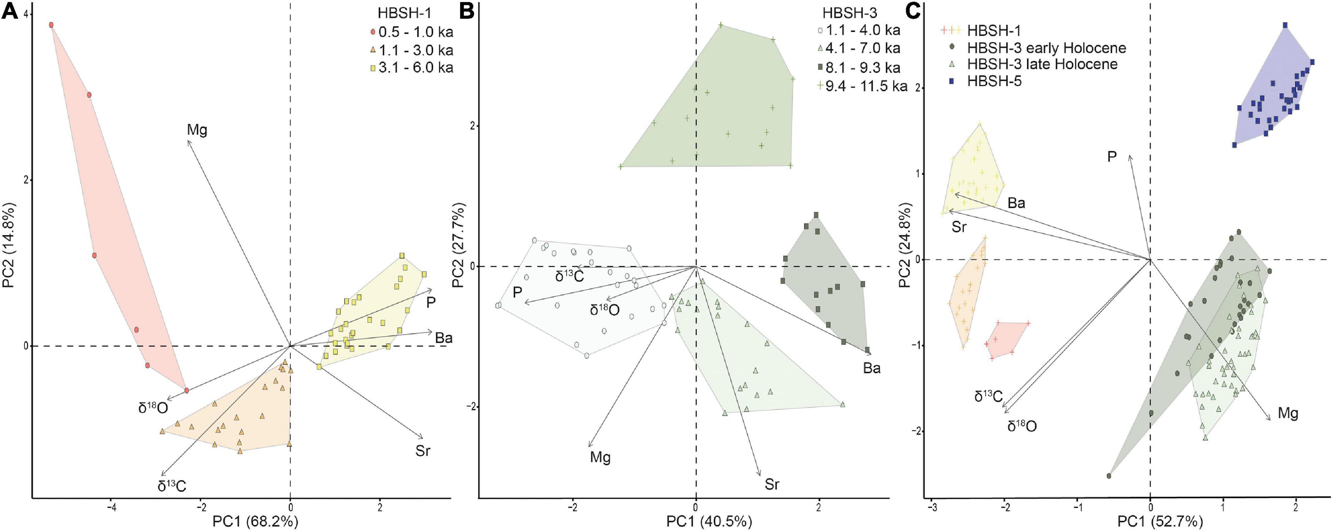
Figure 7. Principal components (PCs) for stalagmites (A) HBSH-1, (B) HBSH-3, and (C) HBSH-1, HBSH-3 and HBSH-5. Since HBSH-5 did not pass the Kaiser-Meyer-Olkin test, only individual PCs for HBSH-1 and HBSH-3 are shown. Data points which are clearly separated from each other are grouped together with the same color.

FIGURE 8

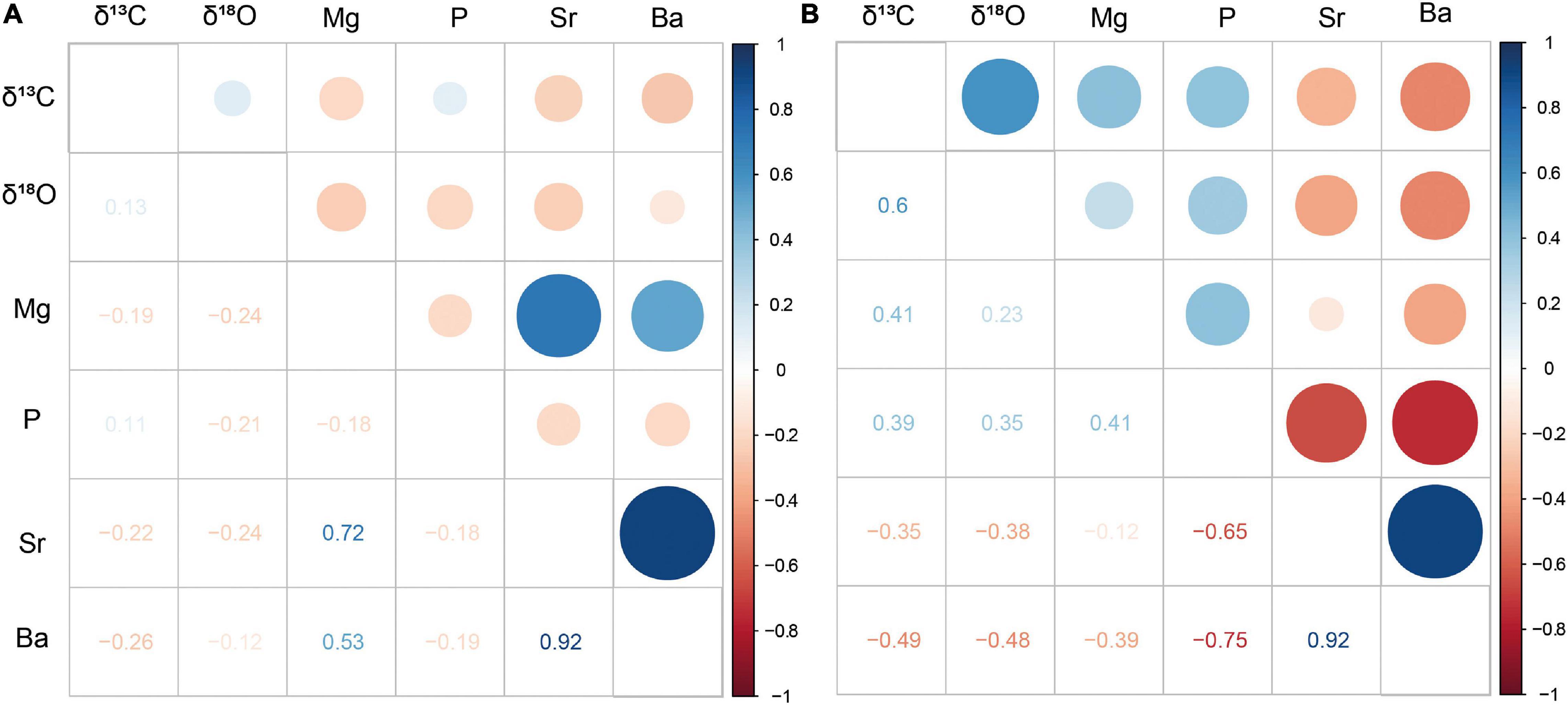
Figure 8. Correlation matrix of centennial means for stable carbon and oxygen isotopes and trace elements of stalagmite HBSH-3 during the early (A) and late (B) phase of the Holocene. The size of the circles increases with increasing positive/negative correlation.

HBSH-1 shows some obvious differences in the trace element concentrations in comparison to HBSH-3 and HBSH-5 since it consists of aragonite. The Mg concentration is much lower (approximately 200 μg/g) and does not change within the stalagmite apart from some peaks in the last 1 ka. In contrast, Sr values are elevated (500 – 800 μg/g) and show minima in the youngest part, while Mg shows the opposite trend. This is related to thin layers of calcite (Jochum et al., 2012). The PCA (Figure 7A) also confirms this observation, since Mg and Sr vectors show opposite directions. This is mainly attributed to the section < 1.0 ka, where also the trace element data (Figure 4) hint toward thin layers of calcite. In general, Ba, Sr, and P show a decreasing trend toward younger ages and are positively correlated (Supplementary Figure A7). As observed in the younger part of HBSH-3, Mg is negatively correlated with Ba (R = −0.58, p < 5 × 10^–6) and Sr (R = −0.62, p < 5 × 10^–7). This indicates that the younger part is influenced by an additional process as described for HBSH-3. By comparing the trace element distribution between HBSH-1 and HBSH-5, which represent only the younger and older part, respectively, the transition described for HBSH-3 is also visible. HBSH-5 shows a weak positive correlation between Mg and Ba and Sr. In contrast, the younger HBSH-1 stalagmite shows a negative correlation between Mg and Ba (R = −0.58, p < 5 × 10^–6) and Sr (R = −0.62, p < 5 × 10^–7).

Sr Isotopes

Strontium isotopes in speleothems have been successfully applied to assess water availability in the karst system and differences in the relative contributions of host rock and overlying soil due to changes in atmospheric deposition and weathering behavior of soils (e.g., Banner et al., 1994; Zhou et al., 2009; Belli et al., 2017; Weber et al., 2018a). Since HBSH is in close proximity to Bunker Cave and formed within the same limestone (Grebe, 1993, 1994), the host rock is expected to show the same Sr isotope signature. Therefore, the Sr isotope ratios for host rock and overlying soil reported in Weber et al. (2018a) for Bunker Cave with values of ⁸⁷Sr/⁸⁶Sr = 0.70836 ± 0.00006 for the host rock, 0.71893 ± 0.00001 for soil horizon C and 0.7237 ± 0.0003 for soil horizon A are used. All ⁸⁷Sr/⁸⁶Sr ratios of the speleothem samples lie between these end members (Figure 6), and changes in the Sr isotope composition are likely related to changes within this binary mixing system.

Similar to the changes observed for the trace elements, the Sr isotopes show a change in their trend between the early and the later growth phase. While the three studied speleothems show a trend toward less radiogenic Sr isotopes ratios in the first growth phase, shifts are observed for HBSH-3 and HBSH-4. In HBSH-3, the lowest ⁸⁷Sr/⁸⁶Sr is observed at 6.7 ± 0.3 ka, shortly after the onset of the second growth phase. This trend toward lower ⁸⁷Sr/⁸⁶Sr, i.e., the value of the host rock, can be related to a longer residence time of the percolating water in the host rock after the hiatus. Therefore, the influence of the host rock Sr isotope signature increasingly affected the ⁸⁷Sr/⁸⁶Sr ratio of the speleothem. At 6.8 ± 0.3 ka, ⁸⁷Sr/⁸⁶Sr strongly increases toward the growth stop. The same is true for HBSH-4, where a strong increase in ⁸⁷Sr/⁸⁶Sr between 6.5 and 6.0 ka is visible, coherent with a change in growth rate. Again, ⁸⁷Sr/⁸⁶Sr gets more radiogenic toward younger ages. The increasing ⁸⁷Sr/⁸⁶Sr ratios are consistent with the reduced growth rate, as well as the trend toward less negative δ¹³C and δ¹⁸O values and the increase in Mg concentration. Therefore, these factors are likely influenced by the same process, i.e., a decrease in water availability. However, this drying trend is not consistent with the Sr isotope evolution observed in Bunker Cave during the early MIS 3 (Weber et al., 2018a). In this study, two growth phases during early MIS 3 show different environmental conditions. While the early phase is believed to have been warm and humid with enhanced soil formation and a high weathering rate, the second phase was characterized by dry conditions resulting in increased δ¹³C values and Mg concentrations. Strontium isotopes, however, tend toward less radiogenic values.

There are several different processes potentially explaining these differences. Although both cave systems lie in close proximity, the processes in the vadose zone can be highly variably and complex. In addition, environmental conditions during MIS 3 were likely different than during the Holocene. Therefore, changes in the karst system do not necessarily affect two different caves in the same way. While for Bunker Cave increased rainfall is considered to cause an overflow system in the karst reducing the influence of the host rock on the Sr isotope signature and vice versa (Riechelmann et al., 2011; Weber et al., 2018a), this is not necessarily true for HBSH. The ⁸⁷Sr/⁸⁶Sr ratios of the younger speleothem generation in HBSH, which suggests apparently drier conditions, may have been influenced in different ways, for instance due to changes in the relative portion of host-rock and soil-derived Sr. Thus, although the drip sites in HBSH might have been influenced by less recharge, this may not be related to drier conditions in the catchment. In Bunker Cave, no drying trend during the Holocene was observed (Fohlmeister et al., 2012). Therefore, it is unlikely that changes in precipitation amount are responsible for the drying observed in HBSH. In contrast, changes in hydrological pathways might have caused this trend in the younger part. Consequently, the climatic conditions were still favorable and were potentially decoupled from the cave conditions.

Within-Cave Correlation of Speleothem Records From HBSH and Bunker Cave

To evaluate the significance of a single speleothem stable isotope record within HBSH, the centennial means are used to calculate correlations between the four samples, the PCA, as well as the two δ¹³C and δ¹⁸O time series (Figures 5, 7, 9, 10A). In general, the stable isotope records of the individual speleothems are highly positive correlated with the respective stack. This proves that the stack still captures the trends observed in the stalagmites. In addition, the δ¹⁸O values of all four stalagmites are positively correlated with each other, suggesting a common forcing. The same is true for the δ¹³C values. However, differences are observed when comparing the δ¹³C and δ¹⁸O values within HBSH. While the δ¹⁸O record of HBSH-5 is positively correlated with the δ¹³C records of the other speleothems, the δ¹³C record of HBSH-5 is negatively correlated with all δ¹⁸O records, as well as the δ¹⁸O HBSH stack. This observation further supports the transition within the Holocene, as described in the previous sections. HBSH-5 only grew during the early phase and shows the initial decrease in δ¹³C at the onset of the Holocene. Thus, this specimen does not record the transition. The δ¹³C and δ¹⁸O stacks are weakly positively correlated (R = 0.33, p < 5 × 10^–4). However, this correlation is mainly caused by the same trend in the youngest section, which is strongly expressed by the positive correlation between the δ¹³C stack and the δ¹⁸O record of HBSH-1 (R = 0.65, p < 8 × 10^–8) and the δ¹⁸O stack and the δ¹³C record of HBSH-1 (R = 0.69, p < 4 × 10^–9).

FIGURE 9

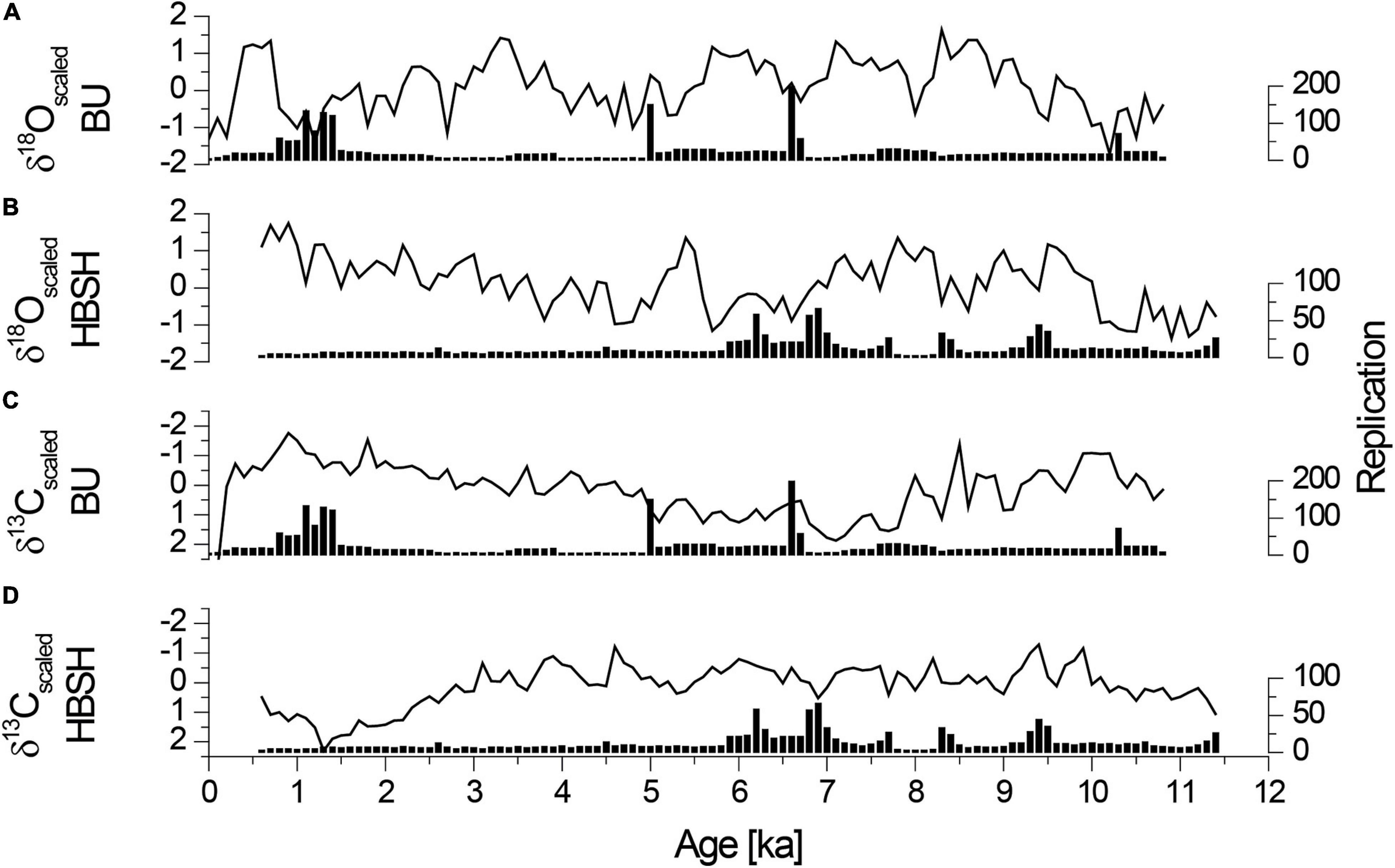
Figure 9. Scaled stable isotope stacks for (A) δ¹⁸O values from Bunker Cave, (B) δ¹⁸O values from HBSH, (C) δ¹³C values from Bunker Cave, and (D) δ¹³C values from HBSH. For all stacks, the replication indicates the number of stable isotope measurements averaged for the centennial mean for the specific time interval. Note that the axes for δ¹³C are inverted to match the plots shown in Figures 4, 5.

FIGURE 10

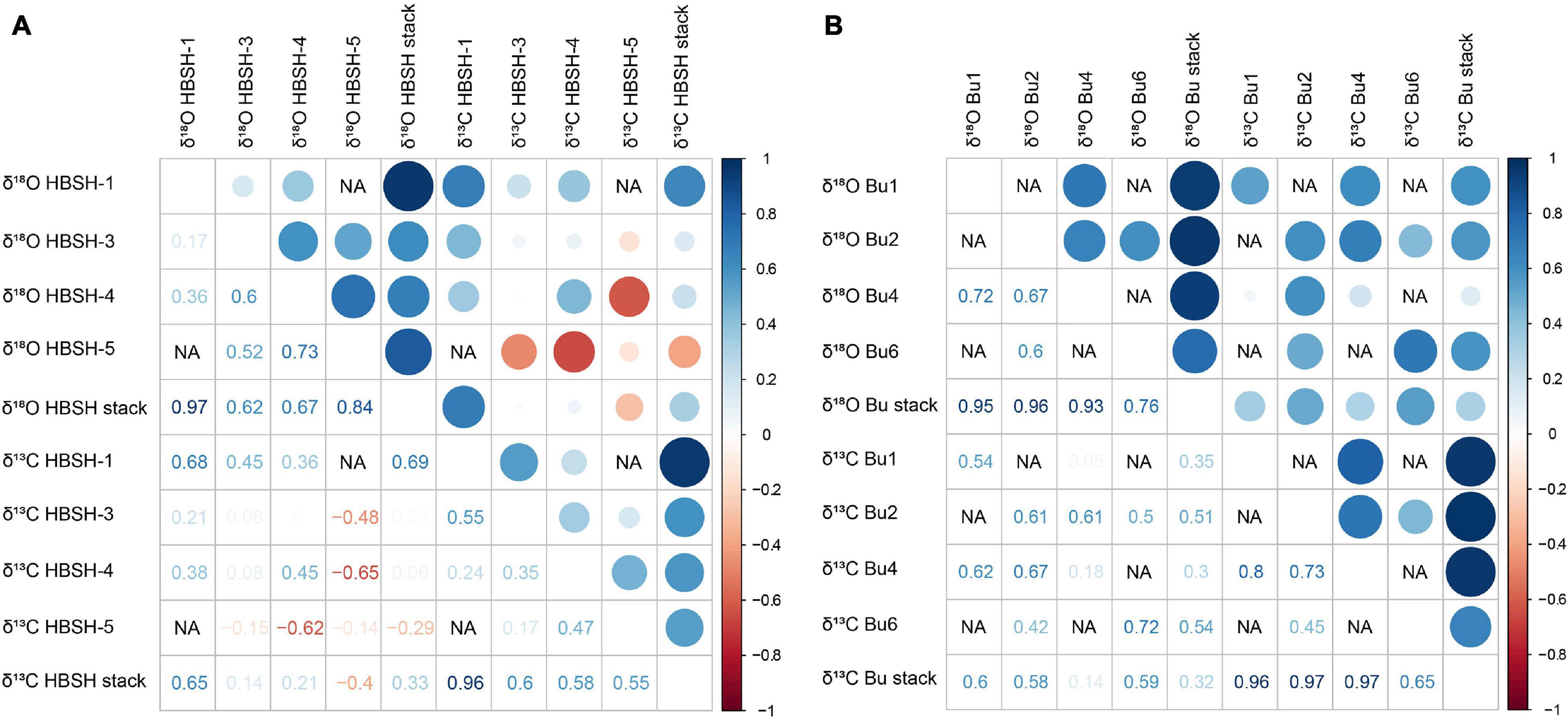
Figure 10. δ¹⁸O and δ¹³C correlation matrix for centennial means of (A) the four HBSH stalagmites, as well as the two HBSH stacks and (B) the four Holocene stalagmites (Fohlmeister et al., 2012) and two stacks from Bunker Cave (Bu). The size of the circles increases with increasing positive/negative correlation.

The PCA including HBSH-1, HBSH-3, and HBSH-5 (Figure 7C) shows a clear separation between the three stalagmites, without any overlap. In addition, a further separation within HBSH-1 and in HBSH-3 is visible. In principle, both stable isotope values separate HBSH-1 and HBSH-5 from each other and show a strong anti-correlation. While HBSH-5 groups together, HBSH-1 is separated in three different clusters (Figures 7A,C). HBSH-3 is the only stalagmite in the PCA which covers almost the whole Holocene and where differences between the early and late growth phase (Figure 8) are expected. The PCA confirms that Mg, Sr and Ba are the main separators for this sample and that δ¹³C and δ¹⁸O start to diverge during the late Holocene (Figure 7B). The overall separation between the three stalagmites shows that each is dependent of other processes, i.e., the difference between aragonite and calcite, as well as the time of formation.

In contrast to HBSH, the correlation matrix for Bunker Cave (Figure 10B) shows positive correlations between all stalagmites and isotope curves, covering the same time interval. This indicates that these two isotope systems were influenced by similar processes, as all individual samples show a positive correlation with the δ¹³C and δ¹⁸O stacks, for the same as well as for the other isotope.

Inter-Cave Correlation of Speleothem Records From HBSH and Bunker Cave

The two δ¹⁸O stacks for HBSH and Bunker Cave are not significantly correlated (Figures 9, 11A). This is largely related to differences in the correlations of individual speleothems. While Bu2 and Bu6 show positive but insignificant correlations with all HBSH stalagmites covering the same time span, Bu4 does not show any correlation with HBSH specimens. Bu1 even shows negative correlations with the HBSH δ¹⁸O records. This indicates, that the Bu speleothems do not show an overall common δ¹⁸O trend as described for HBSH. However, the Bunker Cave speleothems do not overlap as much as the HBSH speleothems in their growth history. Thus, the resulting Bunker Cave stack is largely influenced by stalagmite Bu4, which grew from 8 ka until recent times. Since Bu4 does not show any correlation with the HBSH speleothems, the lack of correlation between the HBSH and the Bunker Cave stacks is reasonable. These findings further support the strong transition in the HBSH records during the middle Holocene. The positive correlation of Bu2 and Bu6 during the early Holocene shows that during that time the records from both caves capture a common signal. However, since Bu4 and Bu1 started to grow around 8 and 6 ka, respectively, both stalagmites mainly cover periods when HBSH is expected to be already influenced by cave-specific processes.

FIGURE 11

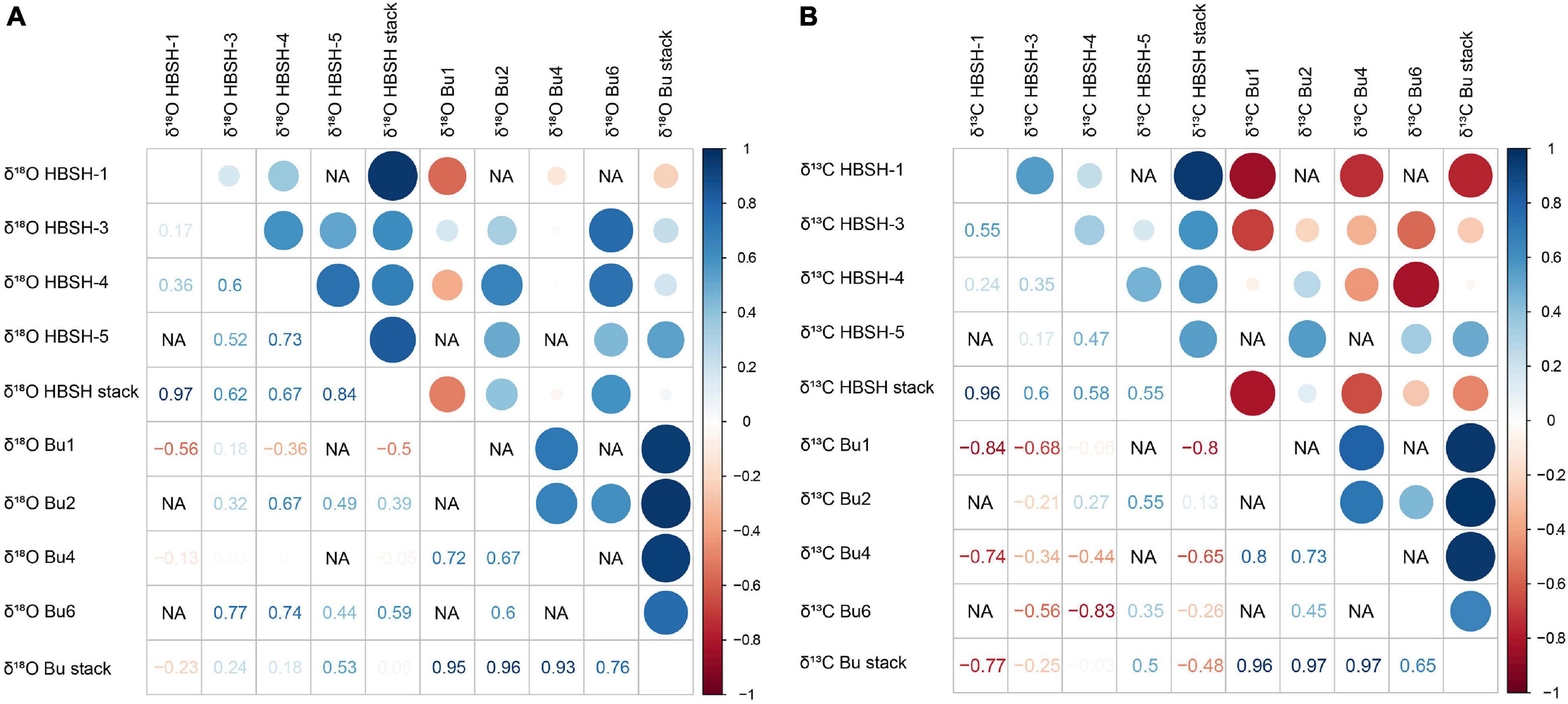
Figure 11. (A) Correlation matrix of centennial means for δ¹⁸O of the four Bu (Fohlmeister et al., 2012) and HBSH stalagmites, as well as the two HBSH and Bu stacks. (B) As for (A) for the δ¹³C values. The size of the circles increases with increasing positive/negative correlation.

For the δ¹³C records (Figure 11B), the comparison between the two cave systems yielded significantly negative correlations. This is especially true for HBSH-1 and the coeval stalagmites Bu1 (R = −0.56, p < 2 × 10^–7) and Bu4 (R = −0.74, p < 2 × 10^–10), which grew during the late Holocene. In addition, HBSH-3 shows negative correlations with all Bunker Cave stalagmites, although covering large parts of the Holocene. A different pattern in visible for HBSH-4, which indicates a weak positive correlation with Bu2, which grew during the early Holocene until approximately 8 ka. In contrast, the comparison with Bu4 yielded a negative correlation (R = −0.44, p < 3 × 10^–4). Interestingly, the δ¹³C values of HBSH-5 show a positive correlation with the coeval Bu2 (R = 0.55, p < 3 × 10^–3) stalagmite, which grew during the early Holocene. This indicates, that the early Holocene δ¹³C signal is consistently registered in both HBSH and Bunker Cave, while later on, the δ¹³C trends become dispersed and yield negative correlations. This observation is in agreement with the previously observed transition in the stable isotope, trace element and Sr isotope records.

The comparison of the stable isotope stacks from the two caves (Figure 9) underscores the results of the correlation analysis. For the δ¹⁸O values, the first part of the Holocene shows some common features between HBSH and Bunker Cave speleothems, such as a peak around 9.6 ka and a general trend toward less negative values. However, this pattern disappears or even reverses in the late Holocene, especially for the youngest 3 – 4 ka, where the trends are opposite. Similar patterns can be observed in the δ¹³C stack, with a trend toward more negative δ¹³C values in the first part until ca. 9.5 ka, recorded in both caves. This represents the onset of the Holocene with increased vegetation and soil formation. However, from 7 – 6 ka onward, a pronounced trend of divergence is observed. At 6.5 ka, the δ¹³C values in Bunker Cave become progressively more negative, while the δ¹³C values in HBSH tend toward less negative values after 6 ka, resulting in a strongly negative correlation.

Implications for Speleothem-Based Palaeoclimate Reconstructions

Our results show that the use of stable isotopes for palaeoclimate reconstructions using speleothems may be strongly biased by non-climatic/non-environmental factors. Although HBSH and Bunker Cave are less than 1 km apart, the stable isotope records of stalagmites from these caves lack a consistent pattern for large parts of the Holocene. The speleothems from HBSH show a trend toward less negative δ¹³C values during the last 6 ka. This could be interpreted as a general trend toward drier conditions, less vegetation cover and reduced soil biological activity, associated with a less humid climate. However, by comparing these results with the much more intensively studied Bunker Cave dataset (including both cave monitoring and palaeoclimate studies, e.g., Riechelmann et al., 2011, 2017; Fohlmeister et al., 2012; Weber et al., 2018a) and other well-established climate archives for the same time interval (e.g., Wanner et al., 2008; Fohlmeister et al., 2013; Sirocko et al., 2016), this interpretation is unlikely. Growth rate and the trace element composition of the speleothems suggest that the increase in the δ¹³C values, and probably also the δ¹⁸O values, mainly results from disequilibrium isotope fractionation on the speleothem surface due to increased drip intervals and/or PCP. Besides these general differences between the two cave systems, there are also differences between individual speleothem records from the same cave. While the aragonitic HBSH-1 stalagmite shows a strong positive correlation between the two isotopes, the calcitic HBSH-5 stalagmite yields a slightly negative correlation. Not all speleothems from the same cave grew simultaneously. Monitoring studies of cave systems have shown that not necessarily all drip sites within a cave yielded a geochemically consistent picture. For instance, Musgrove and Banner (2004) showed that the hydro-geochemistry (⁸⁷Sr/⁸⁶Sr, Sr/Ca, and Mg/Ca) of different drip sites in a cave in central Texas is temporally and spatially variable. Other studies showed that also the drip rate of drip sites within the same cave (Ciur-Izbuc Cave, Romania) can be significantly different and decoupled from rainfall (Moldovan et al., 2018). This is further supported by a study identified a chaotic discharge behavior in Cathedral Cave (Australia), which especially influences growth-rate dependent climate proxies (Mariethoz et al., 2012). This highlights the complex interplay between processes in the karst system and the growth dynamics of speleothems. Therefore, reconstructions based on single speleothems should be viewed with caution and replication, as well as a multi-proxy approach together with statistical approaches should be applied to disentangle potential site-specific cave effects from environmental signals.

Conclusion

By comparing stable isotope records from HBSH and the nearby Bunker Cave, both differences between the two caves and within the individual stalagmites from HBSH were identified. While the proxy records show similar trends in both caves for the early Holocene, a diverging pattern, especially in the δ¹³C values was observed during the late Holocene. By using a multi-proxy approach of stable isotopes, trace elements and Sr isotopes, it is possible to show that the younger part in HBSH was largely influenced by a drying of the karst system, causing an increase in δ¹³C and δ¹⁸O values due to disequilibrium fractionation and PCP. This shows that individual stalagmites may faithfully capture climatic and environmental signals, while stalagmites from other parts of the same cave may be strongly influenced by highly localized cave-internal processes. Replicating stalagmite records and applying several proxies is therefore essential to obtain robust palaeoclimate information.

Data Availability Statement

The original contributions presented in the study are included in the article and Supplementary Material, further inquiries can be directed to the corresponding author.

Author Contributions

MW, DS, and YH designed the study. MW, YH, DS, BS, and CS performed the stable isotope analysis and interpretation. MW, YH, DS, DH, and KJ was performed dating of the samples. YH, KJ, and DS performed Trace element analysis and data evaluation. MW performed Strontium isotope analysis and the regression analysis, and wrote the manuscript, DS, BS, CS, DR, and KJ improved the manuscript. All authors discussed the results and commented on the manuscript.

Funding

MW, KJ, and DS are grateful to the Max Planck Graduate Center and the German Research Foundation (DFG SCHO 1274/9-1 and SCHO 1274/11-1) for funding.

Conflict of Interest

The authors declare that the research was conducted in the absence of any commercial or financial relationships that could be construed as a potential conflict of interest.

Acknowledgments

We thank B. Schwager, B. Stoll, U. Weis, M. Wimmer, M. Maus, and M. Großkopf for assistance in the laboratory and K. Weber for discussion of the PCA. Detailed and constructive comments and suggestions of two reviewers and the editor are greatly acknowledged.

Supplementary Material

The Supplementary Material for this article can be found online at: https://www.frontiersin.org/articles/10.3389/feart.2021.642651/full#supplementary-material

References

Bajo, P., Hellstrom, J., Frisia, S., Drysdale, R., Black, J., Woodhead, J., et al. (2016). “Cryptic” diagenesis and its implications for speleothem geochronologies. Quat. Sci. Rev. 148, 17–28. doi: 10.1016/j.quascirev.2016.06.020

CrossRef Full Text | Google Scholar

Banner, J. L., Musgrove, M., and Capo, R. C. (1994). Tracing ground-water evolution in a limestone aquifer using Sr isotopes: effects of multiple sources of dissolved ions and mineral-solution reactions. Geology 22, 687–690. doi: 10.1130/0091-7613(1994)022<0687:TGWEIA>2.3.CO;2

CrossRef Full Text | Google Scholar

Banner, J. L., Musgrove, M. L., Asmerom, Y., Edwards, R. L., and Hoff, J. A. (1996). High-resolution temporal record of holocene ground-water chemistry: tracing links between climate and hydrology. Geology 24, 1049–1053. doi: 10.1130/0091-7613(1996)024<1049:HRTROH>2.3.CO;2

CrossRef Full Text | Google Scholar

Bartlett, M. S. (1937). Properties of sufficiency and statistical tests. Proc. R. Soc. Lond. Ser. A Math. Phys. Sci. 160, 268–282. doi: 10.1098/rspa.1937.0109

CrossRef Full Text | Google Scholar

Belli, R., Borsato, A., Frisia, S., Drysdale, R., Maas, R., and Greig, A. (2017). Investigating the hydrological significance of stalagmite geochemistry (Mg, Sr) using Sr isotope and particulate element records across the Late Glacial-to-Holocene transition. Geochim. Cosmochim. Acta 199, 247–263. doi: 10.1016/j.gca.2016.10.024

CrossRef Full Text | Google Scholar

Breitenbach, S. F. M., Rehfeld, K., Goswami, B., Baldini, J. U. L., Ridley, H. E., Kennett, D., et al. (2012). COnstructing proxy-record age models (COPRA). Clim. Past 8, 1765–1779. doi: 10.5194/cp-8-1765-2012

CrossRef Full Text | Google Scholar

Budaev, S. V. (2010). Using principal components and factor analysis in animal behaviour research: caveats and guidelines. Ethology 116, 472–480. doi: 10.1111/j.1439-0310.2010.01758.x

CrossRef Full Text | Google Scholar

Budsky, A., Scholz, D., Wassenburg, J. A., Mertz-Kraus, R., Spötl, C., Riechelmann, D. F. C., et al. (2019). Speleothem δ¹³C record suggests enhanced spring/summer drought in south-eastern Spain between 9.7 and 7.8 ka–A circum-Western Mediterranean anomaly? Holocene 29, 1113–1133. doi: 10.1177/0959683619838021

CrossRef Full Text | Google Scholar

Burchette, T. P. (1981). European devonian reefs: a review of current concepts and models. SEPM Special Publ. 30, 85–142. doi: 10.2110/pec.81.30.0085

PubMed Abstract | CrossRef Full Text | Google Scholar

Cheng, H., Edwards, R. L., Hoff, J., Gallup, C. D., Richards, D. A., and Asmerom, Y. (2000). The half-lives of uranium-234 and thorium-230. Chem. Geol. 169, 17–33. doi: 10.1016/S0009-2541(99)00157-6

CrossRef Full Text | Google Scholar

Cheng, H., Lawrence Edwards, R., Shen, C.-C., Polyak, V. J., Asmerom, Y., Woodhead, J., et al. (2013). Improvements in ²³⁰Th dating, ²³⁰Th and ²³⁴U half-life values, and U–Th isotopic measurements by multi-collector inductively coupled plasma mass spectrometry. Earth Planet. Sci. Lett. 371–372, 82–91. doi: 10.1016/j.epsl.2013.04.006

CrossRef Full Text | Google Scholar

Comas-Bru, L., Rehfeld, K., Roesch, C., Amirnezhad-Mozhdehi, S., Harrison, S. P., Atsawawaranunt, K., et al. (2020). SISALv2: a comprehensive speleothem isotope database with multiple age–depth models. Earth Syst. Sci. Data 12, 2579–2606. doi: 10.5194/essd-12-2579-2020

CrossRef Full Text | Google Scholar

Deininger, M., Fohlmeister, J., Scholz, D., and Mangini, A. (2012). Isotope disequilibrium effects: the influence of evaporation and ventilation effects on the carbon and oxygen isotope composition of speleothems – A model approach. Geochim. Cosmochim. Acta 96, 57–79. doi: 10.1016/j.gca.2012.08.013

CrossRef Full Text | Google Scholar

Dettman, D. L., and Lohmann, K. C. (1995). Microsampling carbonates for stable isotope and minor element analysis; physical separation of samples on a 20 micrometer scale. J. Sediment. Res. 65, 566–569. doi: 10.1306/D426813F-2B26-11D7-8648000102C1865D

CrossRef Full Text | Google Scholar

Dreybrodt, W., Hansen, M., and Scholz, D. (2016). Processes affecting the stable isotope composition of calcite during precipitation on the surface of stalagmites: laboratory experiments investigating the isotope exchange between DIC in the solution layer on top of a speleothem and the CO₂ of the cave atmosphere. Geochim. Cosmochim. Acta 174, 247–262. doi: 10.1016/j.gca.2015.11.012

CrossRef Full Text | Google Scholar

Fairchild, I. J., Borsato, A., Tooth, A. F., Frisia, S., Hawkesworth, C. J., Huang, Y., et al. (2000). Controls on trace element (Sr–Mg) compositions of carbonate cave waters: implications for speleothem climatic records. Chemi. Geol. 166, 255–269. doi: 10.1016/S0009-2541(99)00216-8

CrossRef Full Text | Google Scholar

Fairchild, I. J., Smith, C. L., Baker, A., Fuller, L., Spotl, C., Mattey, D., et al. (2006). Modification and preservation of environmental signals in speleothems. Earth Sci. Rev. 75, 105–153. doi: 10.1016/j.earscirev.2005.08.003

CrossRef Full Text | Google Scholar

Fairchild, I. J., and Treble, P. C. (2009). Trace elements in speleothems as recorders of environmental change. Quat. Sci. Rev. 28, 449–468. doi: 10.1016/j.quascirev.2008.11.007

CrossRef Full Text | Google Scholar

Fankhauser, A., Mcdermott, F., and Fleitmann, D. (2016). Episodic speleothem deposition tracks the terrestrial impact of millennial-scale last glacial climate variability in SW Ireland. Quat. Sci. Rev. 152, 104–117. doi: 10.1016/j.quascirev.2016.09.019

CrossRef Full Text | Google Scholar

Fohlmeister, J., Schröder-Ritzrau, A., Scholz, D., Spötl, C., Riechelmann, D. F. C., Mudelsee, M., et al. (2012). Bunker Cave stalagmites: an archive for central European Holocene climate variability. Clim. Past 8, 1751–1764. doi: 10.5194/cp-8-1751-2012

CrossRef Full Text | Google Scholar

Fohlmeister, J., Vollweiler, N., Spötl, C., and Mangini, A. (2013). COMNISPA II: update of a mid-European isotope climate record, 11 ka to present. Holocene 23, 749–754. doi: 10.1177/0959683612465446

CrossRef Full Text | Google Scholar

Genty, D., Blamart, D., Ouahdi, R., Gilmour, M., Baker, A., Jouzel, J., et al. (2003). Precise dating of dansgaard-oeschger climate oscillations in western Europe from stalagmite data. Nature 421, 833–837. doi: 10.1038/nature01391

PubMed Abstract | CrossRef Full Text | Google Scholar

Gibert, L., Scott, G. R., Scholz, D., Budsky, A., Ferràndez, C., Ribot, F., et al. (2016). Chronology for the Cueva Victoria fossil site (SE Spain): evidence for Early Pleistocene Afro-Iberian dispersals. J. Hum. Evol. 90, 183–197. doi: 10.1016/j.jhevol.2015.08.002

PubMed Abstract | CrossRef Full Text | Google Scholar

Grebe, W. (1993). Die bunkerhöhle in iserlohn-letmathe (Sauerland). Mitteilung des Verbands der deutschen Höhlen-und Karstforscher, München 39, 22–23.

Google Scholar

Grebe, W. (1994). Die Hüttenbläserschachthöhle—eine neu entdeckte Höhle in Iserlohn-Letmathe. Mitteilungen & Berichte Speläogruppe Letmathe 10, 49–65.

Google Scholar

Hammerschmidt, E., Niggemann, S., Grebe, W., Oelze, R., Brix, M. R., and Richter, D. K. (1995). Höhlen in Iserlohn.–Schriften zur Karst- und Höhlenkunde in Westfahlen Heft 1, Iserlohn, 154.

Google Scholar

Hansen, M., Scholz, D., Froeschmann, M.-L., Schöne, B. R., and Spötl, C. (2017). Carbon isotope exchange between gaseous CO₂ and thin solution films: artificial cave experiments and a complete diffusion-reaction model. Geochim. Cosmochim. Acta 211, 28–47. doi: 10.1016/j.gca.2017.05.005

CrossRef Full Text | Google Scholar

Hansen, M., Scholz, D., Schöne, B. R., and Spötl, C. (2019). Simulating speleothem growth in the laboratory: determination of the stable isotope fractionation (δ¹³C and δ¹⁸O) between H₂O. DIC and CaCO₃. Chem. Geol. 509, 22–44. doi: 10.1016/j.chemgeo.2018.12.012

CrossRef Full Text | Google Scholar

Hendy, C. H. (1971). The isotopic geochemistry of speleothems—I. The calculation of the effects of different modes of formation on the isotopic composition of speleothems and their applicability as palaeoclimatic indicators. Geochim. Cosmochim. Acta 35, 801–824. doi: 10.1016/0016-7037(71)90127-X

CrossRef Full Text | Google Scholar

Hoffmann, D. L. (2008). 230Th isotope measurements of femtogram quantities for U-series dating using multi ion counting (MIC) MC-ICPMS. Int. J. Mass Spectrom. 275, 75–79. doi: 10.1016/j.ijms.2008.05.033

CrossRef Full Text | Google Scholar

Hoffmann, D. L., Prytulak, J., Richards, D. A., Elliott, T., Coath, C. D., Smart, P. L., et al. (2007). Procedures for accurate U and Th isotope measurements by high precision MC-ICPMS. Int. J. Mass Spectrom. 264, 97–109. doi: 10.1016/j.ijms.2007.03.020

CrossRef Full Text | Google Scholar

Hori, M., Ishikawa, T., Nagaishi, K., Lin, K., Wang, B.-S., You, C.-F., et al. (2013). Prior calcite precipitation and source mixing process influence Sr/Ca, Ba/Ca and ⁸⁷Sr/⁸⁶Sr of a stalagmite developed in southwestern Japan during 18.0-4.5 ka. Chem. Geol. 347, 190–198. doi: 10.1016/j.chemgeo.2013.03.005

CrossRef Full Text | Google Scholar

Jochum, K. P., Scholz, D., Stoll, B., Weis, U., Wilson, S. A., Yang, Q. C., et al. (2012). Accurate trace element analysis of speleothems and biogenic calcium carbonates by LA-ICP-MS. Chem. Geol. 318, 31–44. doi: 10.1016/j.chemgeo.2012.05.009

CrossRef Full Text | Google Scholar

Kaiser, H. F. (1970). A second generation little jiffy. Psychometrika 35, 401–415. doi: 10.1007/BF02291817

CrossRef Full Text | Google Scholar

Kaiser, H. F., and Rice, J. (1974). Little jiffy, mark IV. Educ. Psychol. Meas. 34, 111–117. doi: 10.1177/001316447403400115

CrossRef Full Text | Google Scholar

Köhler, P., Knorr, G., Buiron, D., Lourantou, A., and Chappellaz, J. (2011). Abrupt rise in atmospheric CO2 at the onset of the Bølling/Allerød: in-situ ice core data versus true atmospheric signal. Clim. Past 7, 473–486. doi: 10.5194/cp-7-473-2011

CrossRef Full Text | Google Scholar

Krebs, W. (1974). Devonian carbonate complexes of Central Europe. Soc. Econ. Paleontol. Mineral. Special Publ. 18, 155–208. doi: 10.2110/pec.74.18.0155

PubMed Abstract | CrossRef Full Text | Google Scholar

Lachniet, M. S. (2009). Climatic and environmental controls on speleothem oxygen-isotope values. Quat. Sci. Rev. 28, 412–432. doi: 10.1016/j.quascirev.2008.10.021

CrossRef Full Text | Google Scholar

Lechleitner, F. A., Amirnezhad-Mozhdehi, S., Columbu, A., Comas-Bru, L., Labuhn, I., Pérez-Mejías, C., et al. (2018). The potential of speleothems from Western Europe as recorders of regional climate: a critical assessment of the SISAL database. Quaternary 1:30. doi: 10.3390/quat1030030

CrossRef Full Text | Google Scholar

Li, H.-C., Ku, T.-L., You, C.-F., Cheng, H., Edwards, R. L., Ma, Z.-B., et al. (2005). ⁸⁷Sr/⁸⁶Sr and Sr/Ca in speleothems for paleoclimate reconstruction in Central China between 70 and 280 kyr ago. Geochim. Cosmochim. Acta 69, 3933–3947. doi: 10.1016/j.gca.2005.01.009

CrossRef Full Text | Google Scholar

Lin, Y., Jochum, K. P., Scholz, D., Hoffmann, D. L., Stoll, B., Weis, U., et al. (2017). In-situ high spatial resolution LA-MC-ICPMS 230Th/U dating enables detection of small-scale age inversions in speleothems. Solid Earth Sci. 2, 1–9. doi: 10.1016/j.sesci.2016.12.003

CrossRef Full Text | Google Scholar

Luetscher, M., Boch, R., Sodemann, H., Spotl, C., Cheng, H., Edwards, R. L., et al. (2015). North Atlantic storm track changes during the Last Glacial Maximum recorded by Alpine speleothems. Nat. Commun. 6:6344. doi: 10.1038/ncomms7344

PubMed Abstract | CrossRef Full Text | Google Scholar

Lugli, F., Cipriani, A., Peretto, C., Mazzucchelli, M., and Brunelli, D. (2017). In situ high spatial resolution ⁸⁷Sr/⁸⁶Sr ratio determination of two Middle Pleistocene (c.a. 580 ka) Stephanorhinus hundsheimensis teeth by LA–MC–ICP–MS. Int. J. Mass Spectrom. 412, 38–48. doi: 10.1016/j.ijms.2016.12.012

CrossRef Full Text | Google Scholar

Mangini, A., Verdes, P., Spötl, C., Scholz, D., Vollweiler, N., and Kromer, B. (2007). Persistent influence of the North Atlantic hydrography on central European winter temperature during the last 9000 years. Geophys. Res. Lett. 34:L02704. doi: 10.1029/2006GL028600

CrossRef Full Text | Google Scholar

Mariethoz, G., Baker, A., Sivakumar, B., Hartland, A., and Graham, P. (2012). Chaos and irregularity in karst percolation. Geophys. Res. Lett. 39:L23305. doi: 10.1029/2012GL054270

CrossRef Full Text | Google Scholar

Mattey, D. P., Fairchild, I. J., Atkinson, T. C., Latin, J.-P., Ainsworth, M., and Durell, R. (2010). Seasonal microclimate control of calcite fabrics, stable isotopes and trace elements in modern speleothem from St Michaels Cave. Gibraltar. Geol. Soc. Lond. Special Publ. 336, 323–344. doi: 10.1144/SP336.17

CrossRef Full Text | Google Scholar

Mayewski, P. A., Rohling, E. E., Curt Stager, J., Karlén, W., Maasch, K. A., David Meeker, L., et al. (2004). Holocene climate variability. Quat. Res. 62, 243–255. doi: 10.1016/j.yqres.2004.07.001

CrossRef Full Text | Google Scholar

McArthur, J. M., Howarth, R. J., and Bailey, T. R. (2001). Strontium isotope stratigraphy: LOWESS Version 3: best fit to the marine Sr-Isotope Curve for 0–509 Ma and accompanying look-up table for deriving numerical age. J. Geol. 109, 155–170. doi: 10.1086/319243

CrossRef Full Text | Google Scholar

McDermott, F. (2004). Palaeo-climate reconstruction from stable isotope variations in speleothems: a review. Quat. Sci. Rev. 23, 901–918. doi: 10.1016/j.quascirev.2003.06.021

CrossRef Full Text | Google Scholar

McDermott, F., Frisia, S., Huang, Y., Longinelli, A., Spiro, B., Heaton, T. H. E., et al. (1999). Holocene climate variability in Europe: evidence from δ¹⁸O, textural and extension-rate variations in three speleothems. Quat. Sci. Rev. 18, 1021–1038. doi: 10.1016/S0277-3791(98)00107-3

CrossRef Full Text | Google Scholar

Mickler, P. J., Stern, L. A., and Banner, J. L. (2006). Large kinetic isotope effects in modern speleothems. Geol. Soc. Am. Bull. 118, 65–81. doi: 10.1130/B25698.1

CrossRef Full Text | Google Scholar

Mischel, S. A., Scholz, D., Spötl, C., Jochum, K. P., Schröder-Ritzrau, A., and Fiedler, S. (2017a). Holocene climate variability in Central Germany and a potential link to the polar North Atlantic: a replicated record from three coeval speleothems. Holocene 27, 509–525. doi: 10.1177/0959683616670246

CrossRef Full Text | Google Scholar

Mischel, S. A., Mertz-Kraus, R., Jochum Klaus, P., and Scholz, D. (2017b). TERMITE: an R script for fast reduction of laser ablation inductively coupled plasma mass spectrometry data and its application to trace element measurements. Rapid Commun. Mass Spectrom. 31, 1079–1087. doi: 10.1002/rcm.7895

PubMed Abstract | CrossRef Full Text | Google Scholar

Moldovan, O. T., Constantin, S., and Cheval, S. (2018). Drip heterogeneity and the impact of decreased flow rates on the vadose zone fauna in Ciur-Izbuc Cave. NW Romania. Ecohydrology 11:e2028. doi: 10.1002/eco.2028

CrossRef Full Text | Google Scholar

Moseley, G. E., Spötl, C., Svensson, A., Cheng, H., Brandstätter, S., and Edwards, R. L. (2014). Multi-speleothem record reveals tightly coupled climate between central Europe and Greenland during Marine Isotope Stage 3. Geology 42, 1043–1046. doi: 10.1130/G36063.1

CrossRef Full Text | Google Scholar

Mühlinghaus, C., Scholz, D., and Mangini, A. (2009). Modelling fractionation of stable isotopes in stalagmites. Geochim. Cosmochim. Acta 73, 7275–7289. doi: 10.1016/j.gca.2009.09.010

CrossRef Full Text | Google Scholar

Musgrove, M., and Banner, J. L. (2004). Controls on the spatial and temporal variability of vadose dripwater geochemistry: edwards aquifer, central Texas. Geochim. Cosmochim. Acta 68, 1007–1020. doi: 10.1016/j.gca.2003.08.014

CrossRef Full Text | Google Scholar

Niggemann, S., Mangini, A., Richter, D. K., and Wurth, G. (2003). A paleoclimate record of the last 17,600 years in stalagmites from the B7 cave. Sauerland, Germany. Quat. Sci. Rev. 22, 555–567. doi: 10.1016/S0277-3791(02)00143-9

CrossRef Full Text | Google Scholar

Obert, J. C., Scholz, D., Felis, T., Brocas, W. M., Jochum, K. P., and Andreae, M. O. (2016). ²³⁰Th/U dating of last interglacial brain corals from bonaire (southern Caribbean) using bulk and theca wall material. Geochim. Cosmochim. Acta 178, 20–40. doi: 10.1016/j.gca.2016.01.011

CrossRef Full Text | Google Scholar

Paeckelmann, W. (1922). Der mitteldevonische massenkalk des bergischen landes. Abhandlungen der Preußischen Geologischen Landesanstalt 91, 1–112. doi: 10.5962/bhl.title.134334

PubMed Abstract | CrossRef Full Text | Google Scholar

Paquette, J., and Reeder, R. J. (1995). Relationship between surface structure, growth mechanism, and trace element incorporation in calcite. Geochim. Cosmochim. Acta 59, 735–749. doi: 10.1016/0016-7037(95)00004-J

CrossRef Full Text | Google Scholar

R Core Team (2020). R: A Language and Environment for Statistical Computing. Vienna: R Core Team.

Google Scholar

Richter, D. K., Goll, K., Grebe, W., Niedermayr, A., Platte, A., and Scholz, D. (2015). Weichselzeitliche Kryocalcite als Hinweise für Eisseen in der Hüttenbläserschachthöhle (Iserlohn/NRW). Quat. Sci. J. 64, 67–81. doi: 10.3285/eg.64.2.02

CrossRef Full Text | Google Scholar

Riechelmann, D. F. C., Deininger, M., Scholz, D., Riechelmann, S., Schröder-Ritzrau, A., Spötl, C., et al. (2013). Disequilibrium carbon and oxygen isotope fractionation in recent cave calcite: comparison of cave precipitates and model data. Geochim. Cosmochim. Acta 103, 232–244. doi: 10.1016/j.gca.2012.11.002

CrossRef Full Text | Google Scholar

Riechelmann, D. F. C., Schröder-Ritzrau, A., Scholz, D., Fohlmeister, J., Spötl, C., Richter, D. K., et al. (2011). Monitoring bunker cave (NW Germany): a prerequisite to interpret geochemical proxy data of speleothems from this site. J. Hydrol. 409, 682–695. doi: 10.1016/j.jhydrol.2011.08.068

CrossRef Full Text | Google Scholar

Riechelmann, S., Buhl, D., Schröder-Ritzrau, A., Riechelmann, D. F. C., Richter, D. K., Vonhof, H. B., et al. (2012). The magnesium isotope record of cave carbonate archives. Clim. Past 8, 1849–1867. doi: 10.5194/cp-8-1849-2012

CrossRef Full Text | Google Scholar

Riechelmann, S., Schröder-Ritzrau, A., Spötl, C., Riechelmann, D. F. C., Richter, D. K., Mangini, A., et al. (2017). Sensitivity of Bunker Cave to climatic forcings highlighted through multi-annual monitoring of rain-, soil-, and dripwaters. Chem. Geol. 449, 194–205. doi: 10.1016/j.chemgeo.2016.12.015

CrossRef Full Text | Google Scholar

Scholz, D., and Hoffmann, D. (2008). ²³⁰Th/U-dating of fossil corals and speleothems. Quat. Sci. J. 57, 52–76. doi: 10.3285/eg.57.1-2.3

CrossRef Full Text | Google Scholar

Scholz, D., and Hoffmann, D. L. (2011). StalAge–An algorithm designed for construction of speleothem age models. Quat. Geochronol. 6, 369–382. doi: 10.1016/j.quageo.2011.02.002

CrossRef Full Text | Google Scholar

Scholz, D., Mühlinghaus, C., and Mangini, A. (2009). Modelling δ¹³C and δ¹⁸O in the solution layer on stalagmite surfaces. Geochim. Cosmochim. Acta 73, 2592–2602. doi: 10.1016/j.gca.2009.02.015

CrossRef Full Text | Google Scholar

Scholz, D., Tolzmann, J., Hoffmann, D. L., Jochum, K. P., Spötl, C., and Riechelmann, D. F. C. (2014). Diagenesis of speleothems and its effect on the accuracy of ²³⁰Th/U-ages. Chem. Geol. 387, 74–86. doi: 10.1016/j.chemgeo.2014.08.005

CrossRef Full Text | Google Scholar

Sinclair, D. J., Banner, J. L., Taylor, F. W., Partin, J., Jenson, J., Mylroie, J., et al. (2012). Magnesium and strontium systematics in tropical speleothems from the Western Pacific. Chem. Geol. 29, 1–17. doi: 10.1016/j.chemgeo.2011.10.008

CrossRef Full Text | Google Scholar

Sirocko, F., Knapp, H., Dreher, F., Förster, M. W., Albert, J., Brunck, H., et al. (2016). The ELSA-Vegetation-Stack: reconstruction of landscape evolution zones (LEZ) from laminated eifel maar sediments of the last 60,000 years. Glob. Planet. Change 142, 108–135. doi: 10.1016/j.gloplacha.2016.03.005

CrossRef Full Text | Google Scholar

Steiger, R. H., and Jäger, E. (1977). Subcommission on geochronology: convention on the use of decay constants in geo- and cosmochronology. Earth Planet. Sci. Lett. 36, 359–362. doi: 10.1016/0012-821X(77)90060-7

CrossRef Full Text | Google Scholar

Tooth, A. F., and Fairchild, I. J. (2003). Soil and karst aquifer hydrological controls on the geochemical evolution of speleothem-forming drip waters. Crag Cave, southwest Ireland. J. Hydrol. 273, 51–68. doi: 10.1016/S0022-1694(02)00349-9

CrossRef Full Text | Google Scholar

Treble, P., Shelley, J. M. G., and Chappell, J. (2003). Comparison of high resolution sub-annual records of trace elements in a modern (1911–1992) speleothem with instrumental climate data from southwest Australia. Earth Planet. Sci. Lett. 216, 141–153. doi: 10.1016/S0012-821X(03)00504-1

CrossRef Full Text | Google Scholar

Treble, P. C., Chappell, J., and Shelley, J. M. G. (2005). Complex speleothem growth processes revealed by trace element mapping and scanning electron microscopy of annual layers. Geochim. Cosmochim. Acta 69, 4855–4863. doi: 10.1016/j.gca.2005.06.008

CrossRef Full Text | Google Scholar

von Kamp, H., and Ribbert, K. H. (2005). Erläuterungen zu Blatt 4611 Hagen-Hohenlimburg Geologische Karte von Nordrhein-Westfalen 1: 25.000. Krefeld.

Google Scholar

Wanner, H., Beer, J., Bütikofer, J., Crowley, T. J., Cubasch, U., Flückiger, J., et al. (2008). Mid- to Late Holocene climate change: an overview. Quat. Sci. Rev. 27, 1791–1828. doi: 10.1016/j.quascirev.2008.06.013

CrossRef Full Text | Google Scholar

Warken, S. F., Fohlmeister, J., Schröder-Ritzrau, A., Constantin, S., Spötl, C., Gerdes, A., et al. (2018). Reconstruction of late Holocene autumn/winter precipitation variability in SW Romania from a high-resolution speleothem trace element record. Earth Planet. Sci. Lett. 499, 122–133. doi: 10.1016/j.epsl.2018.07.027

CrossRef Full Text | Google Scholar

Wassenburg, J. A., Dietrich, S., Fietzke, J., Fohlmeister, J., Jochum, K. P., Scholz, D., et al. (2016a). Reorganization of the North Atlantic Oscillation during early Holocene deglaciation. Nat. Geosci. 9, 602–605. doi: 10.1038/ngeo2767

CrossRef Full Text | Google Scholar

Wassenburg, J. A., Scholz, D., Jochum, K. P., Cheng, H., Oster, J., Immenhauser, A., et al. (2016b). Determination of aragonite trace element distribution coefficients from speleothem calcite-aragonite transitions. Geochim. Cosmochim. Acta 190, 347–367. doi: 10.1016/j.gca.2016.06.036

CrossRef Full Text | Google Scholar

Weber, M., Lugli, F., Jochum, K. P., Cipriani, A., and Scholz, D. (2018b). Calcium carbonate and phosphate reference materials for monitoring bulk and microanalytical determination of Sr Isotopes. Geostand. Geoanal. Res. 42, 77–89. doi: 10.1111/ggr.12191

CrossRef Full Text | Google Scholar

Weber, M., Scholz, D., Schröder-Ritzrau, A., Deininger, M., Spötl, C., Lugli, F., et al. (2018a). Evidence of warm and humid interstadials in central Europe during early MIS 3 revealed by a multi-proxy speleothem record. Quat. Sci. Rev. 200, 276–286. doi: 10.1016/j.quascirev.2018.09.045

CrossRef Full Text | Google Scholar

Weber, M., Wassenburg, J. A., Jochum, K. P., Breitenbach, S. F. M., Oster, J., and Scholz, D. (2017). Sr-isotope analysis of speleothems by LA-MC-ICP-MS: high temporal resolution and fast data acquisition. Chem. Geol. 468, 63–74. doi: 10.1016/j.chemgeo.2017.08.012

CrossRef Full Text | Google Scholar

Wedepohl, H. K. (1995). The composition of the continental crust. Geochim. Cosmochim. Acta 59, 1217–1232. doi: 10.1016/0016-7037(95)00038-2

CrossRef Full Text | Google Scholar

Yang, Q., Scholz, D., Jochum, K. P., Hoffmann, D. L., Stoll, B., Weis, U., et al. (2015). Lead isotope variability in speleothems—A promising new proxy for hydrological change? First results from a stalagmite from western Germany. Chem. Geol. 396, 143–151. doi: 10.1016/j.chemgeo.2014.12.028

CrossRef Full Text | Google Scholar

Zhou, H., Feng, Y.-X., Zhao, J.-X., Shen, C.-C., You, C.-F., and Lin, Y. (2009). Deglacial variations of Sr and ⁸⁷Sr/⁸⁶Sr ratio recorded by a stalagmite from Central China and their association with past climate and environment. Chem. Geol. 268, 233–247. doi: 10.1016/j.chemgeo.2009.09.003

CrossRef Full Text | Google Scholar