Modelling Settling-Driven Gravitational Instabilities at the Base of Volcanic Clouds Using the Lattice Boltzmann Method

Introduction

Explosive volcanic eruptions can inject large quantities of ash into the atmosphere, generating multiple hazards at various spatial and temporal scales (Blong, 2000; Bonadonna et al., 2021). Subsequent volcanic ash dispersal and sedimentation can strongly disrupt air traffic (Guffanti et al., 2008; Prata and Rose, 2015), affect inhabited areas (Spence et al., 2005; Jenkins et al., 2015), and impact ecosystems and public health (Gudmundsson, 2011; Wilson et al., 2011). A good understanding of ash dispersal is critical for effective forecasting and management of the response to these hazards. Modern volcanic ash transport and dispersal models have now reached high levels of sophistication (Jones et al., 2007; Bonadonna et al., 2012; Folch, 2012; Folch et al., 2020; Prata et al., 2021) but do not include all of the physical processes affecting ash transport, such as particle aggregation and settling-driven gravitational instabilities (e.g., Durant, 2015). Various studies have highlighted the need to take these processes into account by revealing discrepancies between field measurements and numerical models (Scollo et al., 2008), premature sedimentation of fine ash leading to bimodal grainsize distributions not only related to particle aggregation (Bonadonna et al., 2011; Manzella et al., 2015; Watt et al., 2015) and significant depletion of airborne fine ash close to the source (Gouhier et al., 2019).

Alongside particle aggregation, settling-driven gravitational instabilities contribute to the early deposition of fine ash with similar outcomes (e.g., grainsize bimodality, premature sedimentation of fine ash). These instabilities generate downward-moving ash columns (fingers) which grow from the base of the ash cloud (Figure 1) (Carazzo and Jellinek, 2012; Manzella et al., 2015; Scollo et al., 2017). This phenomenon has the potential to enhance the sedimentation rate of fine ash beyond the terminal fall velocity of individual particles, reducing the residence time of fine ash in the atmosphere. Thus, a rigorous understanding of these processes is important in order to build a comprehensive parametrisation that can be included in dispersal models (Scollo et al., 2010; Bonadonna et al., 2012; Folch, 2012; Durant, 2015).

FIGURE 1

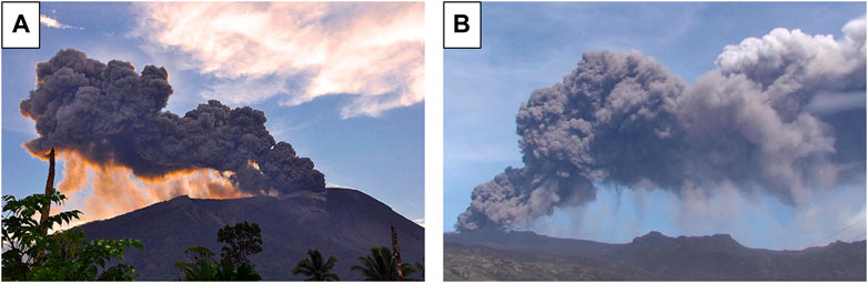
FIGURE 1. Gravitational instabilities observed at the base of a volcanic plume during (A) the 2011 Gamalama eruption (Indonesia) (Credit: AP) and (B) the 2010 eruption of Eyjafjallajökull (Iceland) (Manzella et al., 2015).

Settling-driven gravitational instabilities should be fully characterized as they also have the potential to impact other ash-related processes. First, the high particle concentration and the turbulence induced by fingers (i.e., the intrinsic turbulence within fingers as well as the shear generated during the downward motion) may enhance particle aggregation by increasing the collision rate of particles (Costa et al., 2010; Scollo et al., 2017). This process could happen regardless of plume height and atmospheric conditions contrary to ice-nucleation for example, which requires specific conditions (Maters et al., 2020). Second, as settling-driven gravitational instabilities trigger premature deposition of fine ash, this may affect the residence time of other elements in the plume. Indeed, fine ash is involved in some geochemical processes such as the adsorption of volatiles (e.g., sulphur or halogens) (Bagnato et al., 2013; Zhu et al., 2020). Considering that the sedimentation rate of volatiles depends on the sedimentation rate of fine ash, the possible premature deposition of volatiles can be explained by the presence of both settling-driven gravitational instabilities and particle aggregation. Finally, fine ash has been shown to play an important role in the volcanic cloud heating through radiative processes that may affect the dynamics (Niemeier et al., 2009; Stenchikov et al., 2021). Thus, in order to model the large-scale transport of volcanic clouds, there is a need to estimate accurately the amount of fine ash within the cloud, and, therefore, to constrain all size-selective sedimentation processes such as settling-driven gravitational instabilities.

Settling-driven gravitational instabilities occur at the interface between an upper, buoyant particle suspension, e.g., a volcanic ash cloud, and a lower, denser fluid, e.g., the underlying atmosphere (Hoyal et al., 1999; Burns and Meiburg, 2012; Manzella et al., 2015; Davarpanah Jazi and Wells, 2016). Whilst the initial density configuration is stable, particle settling across the density interface creates a narrow unstable region called the particle boundary layer (PBL) (Carazzo and Jellinek, 2012). Once this attains a critical thickness (Hoyal et al., 1999), a Rayleigh-Taylor-like instability (Chandrasekhar, 1961; Sharp, 1984) can form on the interface between the PBL and the lower layer, generating finger-like structures which propagate downwards. A further critical condition for instability is that the particle settling velocity $V_s$ must be smaller than the finger propagation velocity $V_f$ (Carazzo and Jellinek, 2012). Thus, the occurrence of the instability enhances the sedimentation rate (Manzella et al., 2015; Scollo et al., 2017). Alternatively, if $V_s$ is greater than the propagation velocity of fingers $V_f$, then particles settle individually before a PBL can form and no instability occurs.

Settling-driven gravitational instabilities have been widely studied in laboratory experiments that simulate various natural settings. Many experiments have considered an initial two-layer system, where the particle suspension is initially separated from the underlying denser layer by a removable horizontal barrier (Hoyal et al., 1999; Harada et al., 2013; Manzella et al., 2015; Davarpanah Jazi and Wells, 2016; Scollo et al., 2017; Fries et al., 2021) whilst other experiments have involved injection of the suspension into a density-stratified fluid at its neutral buoyancy level (Cardoso and Zarrebini, 2001; Carazzo and Jellinek, 2012). Similar instabilities can also be studied by allowing fine particles to sediment through the free surface between water and air (Carey, 1997; Manville and Wilson, 2004). Additionally, dimensional analysis has been used to predict that the downward propagation velocity of the generated fingers is given by (Hoyal et al., 1999; Carazzo and Jellinek, 2012)

$V_f={\left[g\left(\frac{{\rho }_{PBL}-{\rho }_f}{{\rho }_f}\right)\right]}^{\frac{2}{5}}{\left[\frac{\pi V_s{\delta }_{PBL}^2}{4}\right]}^{\frac{1}{5}},(1)$

where ${\rho }_{PBL}$ is the PBL bulk density, ${\rho }_f$ the underlying fluid density, $g=9.81$ m.s⁻² the gravitational acceleration and ${\delta }_{PBL}$ the PBL thickness, which by analogy with thermal convection (Turner, 1973) is taken to be (Hoyal et al., 1999)

${\delta }_{PBL}={\left(\frac{G{r}_c{\nu }^2}{g\prime }\right)}^{\frac{1}{3}},(2)$

where $g^{\prime }=g\left({\rho }_{PBL}-{\rho }_f\right)/{\rho }_f$, $\nu$ the kinematic viscosity and $G{r}_c$ a critical Grashof number which estimates the ratio of the buoyancy to viscous forces on the fluid (see Supplementary Table S1 for all acronyms and symbols used in this paper). The reduced gravity $g^{\prime }$ describes the change in the gravitational acceleration due to buoyancy forces. Continuing the analogy with thermal convection, it has been proposed that $G{r}_c={10}^3$ (Hoyal et al., 1999), although recent experimental observations suggests $G{r}_c\approx {10}^4$ may be more accurate (Fries et al., 2021). Therefore, for known particle and fluid properties, it is possible to predict whether collective settling will occur and fingers subsequently form using the condition $V_f>V_s$ (Hoyal et al., 1999). According to this relation, the limit between collective and individual settling occurs when $V_f=V_s$. However, the transition is likely to be smooth, with a transitionary regime where both fluid-like and particle-like settling occur at the same time, as suggested by Harada et al. (2013).

For the initial two-layer configuration, Hoyal et al. (1999) also developed a series of analytical mass-balance models predicting the average particle concentration in the lower layer depending on whether the upper and lower layers were convecting or not. In the case of a quiescent upper layer and a convective lower layer (convection initiated by finger propagation), the evolution of the mass of particles in the lower layer $M_2$ depends on the balance between the mass flux of particles arriving from the upper layer ${\dot{M}}_{in}$ and the mass flux of particle leaving by sedimentation ${\dot{M}}_{out}$

$\frac{d{M}_2}{dt}={\dot{M}}_{in}-{\dot{M}}_{out} ,(3)$

where $t$ is time. Assuming that $M_2\left(t\right)=A{h}_2{C}_2\left(t\right)$, where $C_2\left(t\right)$ is the average particle concentration in the lower layer, Hoyal et al. (1999) solved this equation using ${\dot{M}}_{in}=A{V}_s{C}_1\left(0\right)$, ${\dot{M}}_{out}=A{V}_s{C}_2\left(t\right)$ and the initial condition $C_2\left(0\right)=0$. Thus

$C_2\left(t\right)=C_1\left(0\right)\left[1-e^{-\frac{V_s}{h_2}t}\right],(4)$

where $C_1\left(0\right)$ is the initial particle concentration in the upper layer, $h_2$ the lower layer thickness and $A$ the horizontal cross section of the tank.

Further studies of settling-driven gravitational instabilities have taken theoretical approaches, such as using linear stability analyses to predict the growth rate and characteristic wavelengths of the instability at very early stages (Burns and Meiburg, 2012; Yu et al., 2013; Alsinan et al., 2017). Moreover, various numerical models simulating settling-driven gravitational instability have also been developed (Jacobs et al., 2013; Burns and Meiburg, 2014; Yamamoto et al., 2015; Chou and Shao, 2016; Keck et al., 2021). Most numerical approaches to this problem have used continuum-phase models, where the coupling between particles and fluid is strong enough to describe them as a single-phase (Burns and Meiburg, 2014; Yu et al., 2014; Chou and Shao, 2016). This Eulerian description is valid under the assumptions of sufficiently small particles and a large enough number of particles such that the drag and gravitational forces are in equilibrium. The condition on the particle size can be quantified through the Stokes number (Burgisser et al., 2005; Roche and Carazzo, 2019), one possible definition of which is

$St=\frac{{\rho }_p{D}_p^{2}U}{18\mu L},(5)$

where ${\rho }_p$ is the particle density, $D_p$ the particle diameter, $\mu$ the dynamic viscosity and $U$ and $L$ characteristic velocity and length scales of the flow. For $St<1$, the particles and fluid can be considered coupled and, providing there are enough particles, the continuum approach is valid.

The Eulerian description can be extended to multiple phases in order to simulate their interaction (e.g., gas-liquid interaction) using adaptive mesh refinements to resolve the phase interfaces (Jacobs et al., 2013). However, for large particle diameters and small particle volume fractions, collective behaviour no longer occurs and the continuum-phase method cannot be applied. In this case, there is a need to explicitly model particle motion, taking the drag force into consideration (Yamamoto et al., 2015; Chou and Shao, 2016).

This paper presents an innovative method to implement a continuum model by coupling the Lattice Boltzmann Method (LBM) with a low-diffusivity finite difference (FD) scheme. This model takes advantage of the LBM capabilities to simulate complex flows through uniform grids and thus, the ease of coupling with finite difference methods. This hybrid model has been validated by comparing the results with those from linear stability analysis and laboratory experiments (Fries et al., 2021). The validated model then allows us to gain new insights into the fundamental processes by exploring experimentally-inaccessible regions of the parameter space. We first describe the general framework and governing equations that describe settling-driven gravitational instabilities, then the configuration of the validatory experiments to which we apply the model. Next, we propose a numerical strategy involving a hybrid model in order to solve the system of equations. We then go on to present the linear stability analysis before finally describing and discussing the results of our simulations.

Materials and Methods

Problem Formulation

The model consists of a three-way coupling between fluid momentum, fluid density, and particle volume fraction, based on the assumption that the particle suspension can be represented by a continuum concentration field. Moreover, the particle drag force is in equilibrium with the gravitational force such that the forcing term in the fluid momentum equation is equivalent to a buoyant force term (Boussinesq approximation), which depends on the particle volume fraction $\varnothing \left(\overrightarrow{x},t\right)$ (Burns and Meiburg, 2014; Yu et al., 2014; Chou and Shao, 2016). $\varnothing \left(\overrightarrow{x},t\right)$ satisfies the advection-diffusion-settling equation

$\frac{\partial \varnothing }{\partial t}+\overrightarrow{\nabla }.\left[\varnothing \left({\overrightarrow{u}}_f-V_s\overrightarrow{e_z}\right)\right]=D_c{\nabla }^2\varnothing ,(6)$

where ${\overrightarrow{u}}_f(\overrightarrow{x}, t)$ is the fluid velocity, $D_c$ the particle diffusion coefficient, $\overrightarrow{e_z}$ the vertical unit vector and $\overrightarrow{x}=(x, y, z)$ the position coordinate. The particle settling velocity $V_s$ can be fixed or allowed to be a function of other parameters. Its formulation will be set later according to the assumptions of the flow configuration. The fluid is considered incompressible, meaning $\overrightarrow{\nabla }.{\overrightarrow{u}}_f=0$. Thus, Eq. 6 becomes

$\frac{\partial \varnothing }{\partial t}+\left({\overrightarrow{u}}_f-V_s\overrightarrow{e_z}\right).\overrightarrow{\nabla }\varnothing -\varnothing \overrightarrow{\nabla }.\left(V_s\overrightarrow{e_z}\right)=D_c{\nabla }^2\varnothing .(7)$

The particle settling velocity depends on the ambient fluid density $\rho$, which in turn depends on any transported density-altering properties, such as temperature or the concentration of a chemical species, e.g., the sugar in our validatory experiments (Fries et al., 2021). We incorporate the effect of a single density-altering property on the fluid density through a classical advection-diffusion equation

$\frac{\partial \rho \left({\rho }_0,S\right)}{\partial t}+{\overrightarrow{u}}_f.\overrightarrow{\nabla }\rho \left({\rho }_0,S\right)=D{\nabla }^2\rho \left({\rho }_0,S\right),(8)$

where ${\rho }_0$ is a reference density of the carrier fluid, $S$ the density-altering quantity (temperature or concentration), and $D$ the associated diffusion coefficient. Additionally, under the Boussinesq approximation, we assume that the density depends linearly on $S$. The fluid momentum is modelled with the incompressible Navier-Stokes momentum equation

$\frac{\partial {\overrightarrow{u}}_f}{\partial t}+\left({\overrightarrow{u}}_f.\overrightarrow{\nabla }\right){\overrightarrow{u}}_f=-\frac{1}{{\rho }_0}\overrightarrow{\nabla }p+\nu {\nabla }^2{\overrightarrow{u}}_f+\overrightarrow{F},(9)$

where $p$ is the pressure and $\overrightarrow{F}$ the buoyant body force term. We complete the system of equations by taking this force term to be a function of $\varnothing$ and $\rho$

$\overrightarrow{F}=\left[\left(\frac{{\rho }_p-{\rho }_0}{{\rho }_0}\right)\varnothing +\left(\frac{\rho }{{\rho }_0}-1\right)\left(1-\varnothing \right)\right]\overrightarrow{g}.(10)$

The system of equations presented so far assumes that all particles are of uniform size. In order to generalise to systems with polydisperse particle size distributions, we consider $N$ different particle concentration fields ${\varnothing }_i$, where each one is associated with a different size class and individually satisfies Eq. 7. Furthermore, the body force term becomes

$\overrightarrow{F}=\left[\left(\frac{{\rho }_p-{\rho }_0}{{\rho }_0}\right){\varnothing }_{tot}+\left(\frac{\rho }{{\rho }_0}-1\right)\left(1-{\varnothing }_{tot}\right)\right]\overrightarrow{g},(11)$

where

${\varnothing }_{tot}={\displaystyle \sum }_{i=1}^N{\varnothing }_i.(12)$

Flow Configuration and Experiment Description

Full details of the validatory laboratory experiments can be found in Fries et al. (2021) but we summarise the essential details here. The experiments are performed in a configuration identical to that of Manzella et al. (2015) and Scollo et al. (2017) (Figure 2) and consist of a water tank divided into two horizontal layers, initially separated by a removable barrier. The upper layer is an initially mixed particle suspension, which represents the ash cloud, and the lower layer is a dense sugar solution, analogue to the underlying atmosphere. The particles are spherical glass beads with a median diameter of $41.5\pm 0.5 \text{μm}$ (measured using laser diffraction with a Bettersizer S3 Plus) and a density ${\rho }_p$ of $2519.24\pm 0.09 \text{kg}/{\text{m}}^3$ (measured using helium pycnometry UltraPyc 1200e), and are sufficiently small to be well-coupled with the fluid, whilst the initial particle concentration $C_1\left(0\right)$ of the upper layer is varied from $1$ to $10$ g/l (see Table 1 for the conversion to particle volume fraction ${\varnothing }_0$). The lower layer density is kept constant at ${\rho }_f$ = 1008.4 kg/m³ (corresponding to a sugar concentration of $S_0=35$ g/l), always ensuring an initially stable density configuration.

FIGURE 2

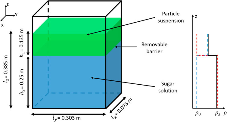
FIGURE 2. Experimental setup used by (Fries et al., 2021) and the initial density profiles associated with the contributions from particles (blue dashed) and sugar (red dotted), as well as the bulk density (black solid). The density of fresh water is given by ${\rho }_0$.

TABLE 1

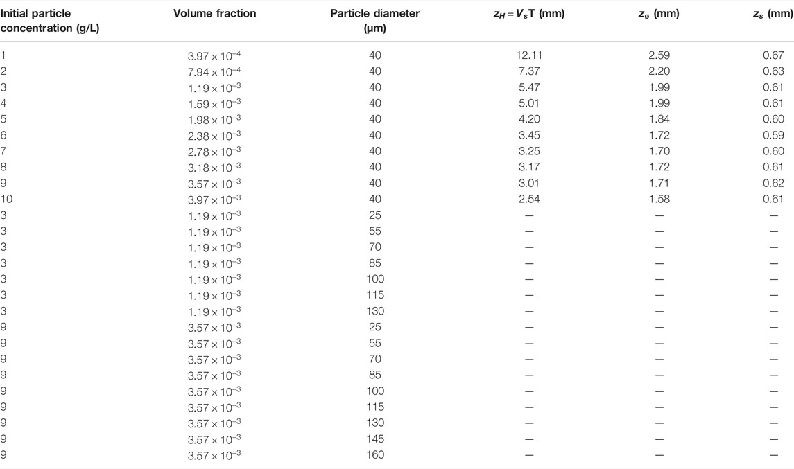
TABLE 1. List of simulations performed. All the simulations have been performed using an initial lower layer fluid density of 1008.4 kg/m³. $z_H$, $z_{\varnothing }$ and $z_s$ are parameters used in the linear stability analysis (LSA) in order to describe the different base states associated with the particle and sugar profiles in Eqs 39, 40. The LSA has been performed only for a constant particle size of 40 µm in order to study the effect of the particle volume fraction.

Before starting an experiment, the upper layer is manually and carefully stirred using a brush. Then the barrier separating the two layers is immediately removed, allowing particle settling through the interface. A PBL subsequently forms and finger formation is initiated. Experiments are illuminated from the side of the water tank with a planar laser and recorded with a high-contrast camera. We measure the vertical finger velocity by tracking the progression of the finger front with time. Additionally, Planar Laser Induced Fluorescence (PLIF) (Koochesfahani, 1984; Crimaldi, 2008) and particle imaging are used to quantify the spatial distribution of the fluid phase density and particle concentration.

Application to Flow Configuration

We apply the general system of equations presented in Problem Formulation section to the configuration of the validatory experiments. The particles are spherical and sufficiently small that their terminal settling velocity in water is given by the Stokes velocity (Stokes, 1851)

$V_s=\frac{D_p^{2}g\left[{\rho }_p-\rho \left(S\right)\right]}{18\mu },(13)$

where $S$ is the sugar concentration and $\rho = {\rho }_0(1+ \alpha S)$, with $\alpha$ the sugar solution expansion coefficient.

The diluted system ensures the Boussinesq assumption is valid as the ratio $\Delta \rho /{\rho }_0$ is much less than 1 (about $6\times {10}^{-3}$ for the highest initial particle volume fraction).

We simulate the solid walls of the tank around our domain with a no-slip boundary condition for the fluid velocity. Neumann boundary conditions are employed for $\varnothing$ and $\rho$ to avoid any flux of particles or sugar across the walls. Thus we impose

$\frac{\partial \varnothing }{\partial x}=0,(14)$

and

$\frac{\partial \rho }{\partial x}=0,(15)$

on the wall nodes. Furthermore, we define the following initial states for $\varnothing$ and $S$:

$\varnothing \left(\overrightarrow{x}, t=0\right)=\{\begin{array}{c}0 , z<H_0\\ {\varnothing }_0 , z>H_0\end{array} ,(16)$

and

$S\left(\overrightarrow{x}, t=0\right)=\{\begin{array}{c}{S}_0, z<H_0\\ 0, z>H_0\end{array},(17)$

where ${\varnothing }_0$ and $S_0$ are the initial particle volume fraction in the upper layer and initial sugar concentration in the lower layer, respectively, and $H_0=0.25$ m the initial height of the interface ($z=0$ corresponds to the base of the tank). We also add a small perturbation to the particle volume fraction field in order to initiate the instability. Finally, the system is initially stationary so ${\overrightarrow{u}}_f\left(\overrightarrow{x}, t=0\right)=0$.

Numerical Methods

The 3D numerical model is implemented using a hybrid strategy where a LBM solves the fluid motion and is coupled with finite difference schemes that solve the advection-diffusion equations for $\varnothing$ and $S$.

Fluid Motion

The LBM is an efficient alternative to conventional Computational Fluid Dynamics (CFD) methods that explicitly solve the Navier-Stokes equations at each node of a discretised domain (He and Luo, 1997; Succi et al., 2010). It is a well-established approach for simulating complex flows, including multiphase fluids (Leclaire et al., 2017) and thermal and buoyancy effects (Parmigiani et al., 2009; Noriega et al., 2013). The LBM originates from the kinetic theory of gases and provides a description of gas dynamics at the mesoscopic scale. This scale exists between the microscopic, which describes molecular dynamics, and the macroscopic, which gives a continuum description of the system with variables such as density and velocity. Thereby, the mesoscopic scale considers a probability distribution function of molecules described by the Lattice Boltzmann equation. This model reduces the process to two main steps: streaming (i.e., displacement of populations between consecutive calculation nodes), and collision (i.e., interaction of populations on a node). The Bhatnagar-Gross-Krook (BGK) model (Bhatnagar et al., 1954) provides a simple collision process based on a fundamental property given by kinetic theory which describes gas motion as a perturbation around the equilibrium state. Then, the LBM-BGK model solves the equation

$f_i\left(\overrightarrow{x}+{\overrightarrow{c}}_i\delta t, t+\delta t\right)-f_i\left(\overrightarrow{x}, t\right)=-\frac{\delta t}{\tau }\left(f_i\left(\overrightarrow{x}, t\right)-f_i^{eq}\right),(18)$

where the particle population $f_i$ is a discrete representation of the probability distribution function, $\delta t$ is the time step, $f_i^{eq}(\rho , {\overrightarrow{u}}_{\mathit{f}})$ the equilibrium distribution function, $\tau$ the relaxation time associated with the flow viscosity and ${\overrightarrow{c}}_i$ the local particle velocity. The LBM is applied to specific types of lattices that describe how the populations move through the calculation nodes (Kruger et al., 2017). These types of lattice are commonly summarized in the form $DrQm$ where $r$ denotes the dimension of the system and $m$ the number of directions in which populations can propagate. Figure 3 shows the scheme $D3Q19$ used for our 3D simulations and the associated set of local velocities.

FIGURE 3

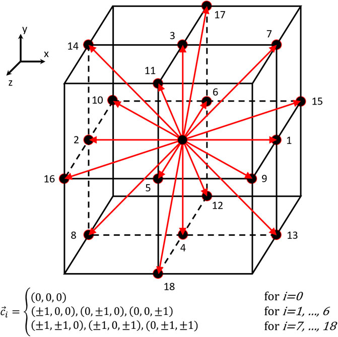
FIGURE 3. Depiction of the D3Q19 lattice. The red arrows show the different possible directions of propagation. The associated local velocities are summarised in the velocity set ${\overrightarrow{c}}_i$.

The macroscopic fluid state is described through the usual macroscopic variables such as density, velocity and kinematic viscosity. These variables are related to the moments of the populations $f_i$ through

$\rho ={\displaystyle \sum }_i{f}_i,(19)$

and

$\rho {\overrightarrow{u}}_f={\displaystyle \sum }_i{f}_i{\overrightarrow{c}}_i,(20)$

whilst the kinematic viscosity controls the relaxation to equilibrium through the relaxation time

$\tau =\frac{\nu }{c_s^2}+\frac{\delta t}{2}.(21)$

The variable $c_s$ is commonly called the speed of sound and is equal to $(1/\sqrt{3})\delta x/\delta t$ where $\delta x$ is the spatial step. However, the classical LBM-BGK model described above does not take into account any forcing term. One way to include forcing is to rewrite Eq. 18 as

$f_i\left(\overrightarrow{x}+{\overrightarrow{c}}_i\delta t, t+\delta t\right)-f_i\left(\overrightarrow{x}, t\right)=-\frac{1}{\tau }\left(f_i\left(\overrightarrow{x}, t\right)-f_i^{eq}\right)+F_i\delta t,(22)$

where $F_i$ is the forcing term, which can be expressed by a power series in the local particle velocities, and the equilibrium distribution is now given by $f_i^{eq}=f_i^{eq}(\rho , {\overrightarrow{u}}_{\mathit{f}}^{\mathit{*}})$, where $\rho {\overrightarrow{u}}_{\mathit{f}}^{\mathit{*}}={\sum }_i{f}_i{\overrightarrow{c}}_i+b\overrightarrow{F}\delta t$. The determination of the coefficient $b$, as well as the power series expansion of $F_i$ are described by Guo et al. (2002). Finally, no-slip boundary conditions in the LBM, to simulate walls for example, can be implemented using the classical bounce-back boundary condition (Kruger et al., 2017) where the populations arriving on a wall node during the streaming step are simply reflected back to their previous nodes.

Transport of Particles and Other Density-Altering Quantities

The particles and other density-altering quantities are described by continuum fields that follow an advection-diffusion law coupled with the fluid motion as simulated with the LBM. The numerical solution of the advection equation is particularly challenging for methods which, like ours, are Eulerian (i.e., mesh-based). Indeed, such methods exhibit numerical diffusion which may strongly reduce model accuracy and, in some cases, even exceed the amplitude of the actual, physical diffusion term. The lack of physical diffusion in our problem and the presence of sharp interfaces restrict our ability to solve the advection equations with the LBM. In fact, the advection-diffusion equation can be solved by the LBM with a BGK approach in analogous fashion to the fluid motion by modifying the equilibrium distribution and the relaxation time to depend on the diffusion coefficient $D$ rather than $\nu$

$\tau =\frac{D}{c_s^2}+\frac{\delta t}{2}.(23)$

However, a stability condition for a LBM-BGK algorithm is $\tau /\delta t>1/2$. Thus, since the problem is convection dominated, the low diffusion coefficient ($D \ll 1$) drives the model towards the stability limit, introducing strong numerical errors near sharp concentration gradients (Hosseini et al., 2017). For this reason, we solve the advection term using two finite-difference schemes which are selected depending on the required accuracy: the classical first-order upwind finite difference and the third-order Weighted Essentially Non Oscillatory (WENO) finite difference scheme (Liu et al., 1994; Jiang and Shu, 1996).

Coupling the LBM with an upwind finite difference scheme allows us to avoid the stability problem. First-order FD schemes however, still suffer from the problem of numerical diffusion due to the truncation error associated with terminating the Taylor expansion after the first spatial derivative. The induced numerical error $NE$ for the convective term in the advection-diffusion equation is given by

$NE\sim u\frac{\delta x}{2}\frac{{\partial }^2\varnothing }{\partial x^2},(24)$

where $u$ is the transport velocity. $NE$ acts like an additional diffusion term because of the presence of the second-order derivative. (A quantitative estimate of the numerical diffusion for both 1st order and WENO procedure is available in section 1.3 of the Supplementary Figure S2). The numerical diffusion associated with the solution of $S$ is negligible due to the low fluid velocity and consequently the use of the first order FD scheme does not significantly affect the accuracy. However, in the solution of $\varnothing$, which includes an additional velocity contribution due to the settling, the truncation error associated with the first-order scheme becomes non-negligible. Whilst decreasing $\delta x$ would reduce numerical diffusion, we would require an unpractically small value in order to get a sufficiently accurate solution. Additionally, simply increasing the order of the scheme introduces dispersion (spurious oscillations) near regions of high gradient, according to the Godunov theorem (Godunov, 1954, 1959). Therefore, we choose here to implement the low diffusive WENO procedure for the solution of $\varnothing$, thus achieving a stable and high-resolution scheme without dispersion.

Further information on how we discretise the convective term in the advection-diffusion equation using the first order upwind and the third order WENO finite difference schemes is detailed in Section 1 of the Supplementary Figure S1.

Numerical Implementation

Our model is implemented using Palabos (Parallel Lattice Boltzmann Solver), a Computational Fluid Dynamics (CFD) solver based on the Lattice Boltzmann Method and developed by the Scientific Parallel Computing group of the Computer Science Department, University of Geneva (Latt et al., 2020). Palabos is designed to perform calculations on massively parallel computers, thus allowing very small spatial resolutions for accurate simulation of the finger dynamics.

Linear Stability Analysis

In order to validate our model, we compare the early-time simulated behaviour against predictions from linear stability analysis (LSA). LSA is applied to the onset of the physical instability at the interface between layers of different particle concentration. It involves defining a field equation-satisfying base state for each of the unknown fields in a problem and then applying an infinitesimally small perturbation to each of these fields. The equations are then expanded to linear order in the perturbation, with higher order terms assumed to be negligible. By assigning the perturbation to have the form of a complex waveform, the system of equations reduces to an eigenvalue problem, which can be solved to determine which wavelengths will grow or decay (Chandrasekhar, 1961). In this section, we assume that the system is invariant under translation in the $x-y$ plane, thus reducing the analysis to a 2D problem. We strongly follow the procedure described by (Burns and Meiburg, 2012) in order to solve our problem.

Nondimensionalisation

We nondimensionalise our system of equations by defining

$l^c={\left(\frac{{\nu }^2}{g}\right)}^{1/3},(25)$

$t^c={\left(\frac{\nu }{g^2}\right)}^{1/3},(26)$

and

$p^c={\rho }_0{\left(\nu g\right)}^{2/3},(27)$

where $l^c$, $t^c$ and $p^c$ are characteristic quantities. We also define the dimensionless parameters

$S^{\ast }=\alpha S_0,(28)$

${\varnothing }^{\ast }={\varnothing }_0,(29)$

$Fr=\frac{1}{t^c} \sqrt{\frac{l^c}{g}},(30)$

and

$S{c}_i=\frac{\nu }{D_i},(31)$

noting that $Fr$ is a Froude number and $S{c}_i$ are Schmidt numbers. Furthermore, the stream function $\psi$ is defined such that ${\overrightarrow{u}}_f=\left(\partial \psi /\partial z, -\partial \psi /\partial x\right)$ and the vorticity as $\overrightarrow{\omega }=\overrightarrow{\nabla }\times {\overrightarrow{u}}_f$. Then, applying the characteristic quantities to the vorticity formulation and Eqs 7–9, we obtain the dimensionless system (for the rest of the analysis, all the symbols used represent dimensionless quantities):

$\omega =-{\nabla }^2\psi .(32)$

$\frac{\partial \omega }{\partial t}+\left({\overrightarrow{u}}_f.\overrightarrow{\nabla }\right)\omega ={\nabla }^2\omega +\frac{\partial \varnothing }{\partial y}\frac{{\varnothing }^{\ast }}{F{r}^2}\left[S{S}^{\ast }-\left(\frac{{\rho }_p-{\rho }_0}{{\rho }_0}\right)\right]-\frac{\partial S}{\partial y}\frac{S^{\ast }}{F{r}^2}\left(1-\varnothing {\varnothing }^{\ast }\right),(33)$

$\frac{\partial S}{\partial t}+{\overrightarrow{u}}_f.\overrightarrow{\nabla }S=\frac{1}{S{c}_s}{\nabla }^{2}S,(34)$

and

$\frac{\partial \varnothing }{\partial t}+\left({\overrightarrow{u}}_f-V_s\overrightarrow{e_z}\right).\overrightarrow{\nabla }\varnothing =\frac{1}{S{c}_c}{\nabla }^2\varnothing .(35)$

Note that here we have neglected the term $-\varnothing \overrightarrow{\nabla }.\left(V_s\overrightarrow{e_z}\right)$ in Eq. 7 assuming the fluid density variation across the interface is sufficiently small that it does not affect the particle settling velocity.

Variable Expansion and Eigenvalue Problem

We linearise the system of equations by expanding each variable in terms of a base state and a perturbation

$\phi \left(y,z,t\right)=\overline{\phi }\left(z\right)+{\phi }^{\prime }\left(y, z, t\right),(36)$

where $\phi \left(y,z,t\right)=\{\psi ,\omega ,\varnothing ,S\}$, $\overline{\phi }\left(z\right)=\{\overline{\psi },\overline{\omega }, \overline{\varnothing },\overline{S}\}$ the associated base state and ${\phi }^{\prime }\left(y, z, t\right)=\{{\psi }^{\prime },{\omega }^{\prime },{\varnothing }^{\prime }, S\prime \}$ the perturbation. We choose the following base states

$\overline{\psi }=0,(37)$

$\overline{\omega }=0,(38)$

$\overline{\varnothing }\left(z, t\right)=\frac{1}{2}\left(1+\text{erf}\left(\frac{z}{z_{\varnothing }\left(T\right)}\right)\right),(39)$

and

$\overline{S}\left(z, t\right)=\frac{1}{2}\left(1-\text{erf}\left(\frac{z-V_{s}t}{z_S\left(T\right)}\right)\right),(40)$

where $z_{\varnothing }\left(T\right)$ and $z_S\left(T\right)$ are coefficients fitted in order to have similar base states to the profiles observed in the simulations prior to the onset of the instability which starts growing at the time $T$. We choose these base states to represent the initial conditions of the validatory experiments; Eqs 37, 38 ensure an initially-zero velocity field whilst the error functions in Eqs 39, 40 ensure sigmoidal distributions for $\overline{S}$ and $\overline{\varnothing }$.

Solutions for the perturbation are assumed to have the form of normal modes

${\phi }^{\prime }\left(y, z, t\right)=\widehat{\phi }\left(z\right)exp\left(iky+\sigma t\right),(41)$

where $\widehat{\phi }\left(z\right)$ is the perturbation amplitude, $k$ the wavenumber and $\sigma$ the instability growth rate. The linearised system of equations is then formulated in matrix form so that the problem is reduced to the eigenvalue problem $K\overrightarrow{x}=\sigma W\overrightarrow{x}$ where

$\overrightarrow{x}=\left(\begin{array}{c}\widehat{\psi }\left(z\right)\\ \widehat{\omega }\left(z\right)\\ \widehat{S}\left(z\right)\\ \widehat{\varnothing }\left(z\right)\end{array}\right),(42)$

and, in a reference frame moving downward at $V_s$, the matrices $K$ and $W$ are given by

$K=\left(\begin{array}{cccc}M& I& 0& 0\\ 0& M-V_s{D}_z& -ik\frac{S^{\ast }}{F{r}^2}\left(1-\overline{\varnothing }{\varnothing }^{\ast }\right)I& ik\frac{{\varnothing }^{\ast }}{F{r}^2}\left[\overline{S}{S}^{\ast }-\left(\frac{{\rho }_p-{\rho }_0}{{\rho }_0}\right)\right]I\\ ik\frac{d\overline{S}}{dz}I& 0& \frac{1}{S{c}_s}M-V_s{D}_z& 0\\ ik\frac{d\overline{\varnothing }}{dz}I& 0& 0& \frac{1}{S{c}_c}M\end{array}\right),(43)$

and

$W=\left(\begin{array}{cccc}0& 0& 0& 0\\ 0& I& 0& 0\\ 0& 0& I& 0\\ 0& 0& 0& I\end{array}\right),(44)$

where $D_z=\partial /\partial z$, $M=-k^2+D_z^2$ and $I$ is the identity operator.

The eigenvalues $\sigma$ determine the stability of the system:

• If all the eigenvalues have negative real parts, the system remains stable

• If at least one eigenvalue has a positive real part, the system is unstable.

In order to solve the eigenvalue problem, the spatial derivatives are discretised using the linear rational collocation method with a grid transformation allowing a fine resolution around narrow interfacial regions (Baltensperger and Berrut, 2001; Berrut and Mittelmann, 2004).

The key result of the LSA is the dispersion relation between $\sigma$ and $k$. Figure 4 presents the growth rate as a function of the wavenumber, for different initial particle volume fractions. The parameters for the different base states used to produce these curves are summarised in Table 1. We use this result in Comparison of Model Results With Predictions From Linear Stability Analysis Section in order to compare the predictions of the LSA with the results of our numerical model. Additionally, a comparison with the 2D Fourier analysis of the interface is given in Supplementary Figures S3–S5.

FIGURE 4

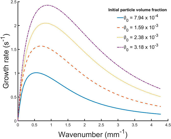
FIGURE 4. Dispersion relation obtained from LSA for several initial particle volume fractions.

Results

We validate our numerical model by comparing the results with predictions from LSA and experimental observations. The LSA predicts the growth rates of different perturbation wavenumbers during the very early stage of the instability, which can be compared with the spectrum of wavenumbers present in the particle concentration interface in the numerical model. Additionally, the experiments of Fries et al. (2021) employ imaging techniques to measure quantities, such as the particle concentration field and finger velocity, at times beyond the linear regime. Finally, our results are compared with some results of previous analyses on settling-driven gravitational instabilities (Hoyal et al., 1999; Carazzo and Jellinek, 2012).

Comparison of Model Results With Predictions From Linear Stability Analysis

In order to compare our 3D simulations with the 2D linear stability analysis, we consider just the central plane of the simulation domain, i.e., a slice in the $(y, z)$ plane located at $x=l_x/2$ ($l_x$ being the tank depth) (Figure 2). We define the front of the particle field to be the lowest position where $\varnothing = {\varnothing }_0/2$ and also define $H\left(y\right)$ to be the separation between $z=0$ and this front. Our study has shown that the front position is only weakly affected when using other possible thresholds, i.e., ${\varnothing }_0/10$ or ${\varnothing }_0/5$ (relative change ∼3%). Figure 5A shows an example of a space-time diagram showing the evolution of $H\left(y\right)$ through time. Furthermore, by calculating the Fourier transform $\tilde{H}\left(k, t\right)$ of $H\left(y\right)$ at different times, we can identify different dominant wavenumbers and their associated amplitudes as shown in the space diagram of the power spectral density (PSD) ${\text{Γ}}_H(k,t)=\left(1/\left(k_S{L}_S\right)\right){\left|\tilde{H}\left(k,t\right)\right|}^2$ (Figure 5B), where $k_S$ is the sampling wavenumber and $L_S$ the number of samples. We extract the dominant mode and its associated growth rate from ${\Gamma }_H(k, t)$ and compare the results with the predicted growth rates from LSA. We apply this analysis during a period when the amplitude $\left|\tilde{H}\left(k,t\right)\right|$ of any given mode does not exceed 40% of its wavelength, thus ensuring we are still in the linear regime (Lewis, 1950).

FIGURE 5

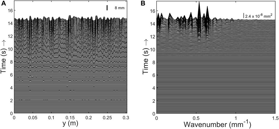
FIGURE 5. (A) Space-time diagram of the particle front height $H(y, t)$. (B) Evolution of the power spectral density of the particle interface over time. Initial particle volume fraction: ${\varnothing }_0=3.97\times {10}^{-4}$

During the linear regime, we can assume that the growth of the spectral amplitude can be described as (Völtz et al., 2001)

$\left|\tilde{H}\left(k,t\right)\right|=\left|\widetilde{H_i}\left(k\right)\right|\text{exp}\left({\sigma }_{sim}\left(k\right)t\right),(45)$

with $\left|\widetilde{H_i}\left(k\right)\right|$ the initial amplitude and ${\sigma }_{sim}\left(k\right)$ the instability growth rate as determined from the simulations. Thus, the PSD can be expressed as

${\mathrm{\Gamma }}_H\left(k, t\right)={\mathrm{\Gamma }}_{Hi}\exp \left(2{\sigma }_{sim}\left(k\right)t\right),(46)$

where ${\Gamma }_{H i}$ is the initial spectral density. At each time step, we extract the PSD and the wavenumber $k_{sim}$ associated with the dominant mode as shown in Figure 6. However, we observe that the dominant mode remains at the same wavenumber during instability growth except for three cases (${\varnothing }_0=$ $1.59\times {10}^{-3}$, $2.38\times {10}^{-3}$ and $3.97\times {10}^{-3}$) where we observed that the dominant mode changed its position in the spectral space. For these simulations only, we have a set of several wavenumbers $k_{sim,i},$ ($i=\mathrm{1,2,3}$) associated with the dominant mode. With the computed PSD of the dominant mode as a function of time ${\text{Γ}}_H\left(k_{sim}, t\right)$, we apply our exponential fitting (Eq. 46) to determine the growth rate ${\sigma }_{sim,i}$ (Figure 6B). For the simulations which resulted in several values of $k_{sim,i}$ for the dominant mode, we measured the growth rates of each mode ${\sigma }_{sim,i}$ and found identical values, up to a precision of 5%. Additionally, for each simulation, we find the time $T$ when the instability starts growing easily identified as the time at which the modal wavenumber becomes non-zero (e.g., in Figure 6A this is at approximately 6 s). At this time, we extract the associated vertical profiles of particle and sugar concentration which are used to find the coefficients $z_{\varnothing }\left(T\right)$ and $z_S\left(T\right)$ (Eqs 39, 40) and thus determine the base states of $\overline{\varnothing }\left(z, T\right)$ and $\overline{S}\left(z, T\right)$ (Figure 7). We then perform the LSA for each ${\varnothing }_0$, using the appropriate base states, and obtain a dispersion relation $\sigma =f\left(k\right)$. Using this relation, we predict the different growth rates $\sigma ={\sigma }_{LSA,i}$ associated with $k=k_{sim,i}$ and we compare with ${\sigma }_{sim}\left(k_{sim,i}\right)$ as measured in our simulations. Figure 8 shows the comparison between ${\sigma }_{sim}$ (black dots) and ${\sigma }_{LSA,i}$ (red triangles), as predicted from the LSA, for the dominant wave mode. The error bars associated with the simulation data show the uncertainty on the fitted results of ${\sigma }_{sim}$ (given by the 95% confidence interval). For the cases including a moving dominant mode, we plotted the growth rates associated with the different measured wavenumbers. We see that the dependence of the largest value of ${\sigma }_{LSA,i}$ on the initial particle concentration is in good agreement with the simulated growth rate.

FIGURE 6

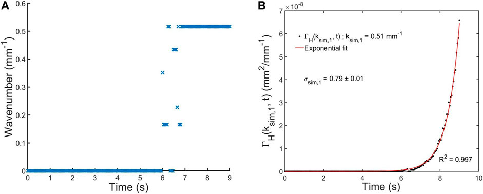
FIGURE 6. (A) Example of dominant wavenumbers extracted from the maximum of the PSD. Initial particle volume fraction ${\varnothing }_0=7.94\times {10}^{-4}$. (B) Exponential fitting to the temporal evolution of the PSD for the first maximum in (A), k_sim,1 = 0.517 mm⁻¹.

FIGURE 7

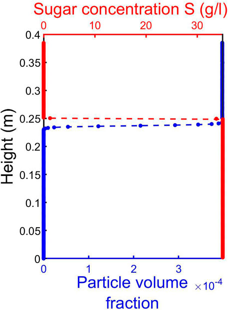
FIGURE 7. Example of LSA base states extracted from the simulations for ${\varnothing }_0=$ $3.97\times {10}^{-4}$. Dots: profiles extracted from the simulations at T = 9.55s (start of the instability growth). Dotted lines: Fit with Eqs 39, 40. i.e., base states used for the LSA. Blue: particle volume fraction. Red: Sugar concentration.

FIGURE 8

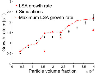
FIGURE 8. Comparison of the instability growth rate measured in the simulations (black circles) and that predicted by the linear stability analysis (red triangles).

Comparison With Experimental Investigations

Figures 9A,B show a qualitative comparison between snapshots taken from experiments (Fries et al., 2021) and simulations (slice in the numerical domain). First, we note that our model is able to qualitatively reproduce the shape and size of fingers, especially their fronts where we observe the formation of lobes and eddies due to the Kelvin-Helmholtz instability (Chou and Shao, 2016). Second, we provide a quantitative validation of the non-linear regime by comparing our model with experiments, through measurements of the PBL thickness and the vertical finger velocity as functions of the particle volume fraction and size.

FIGURE 9

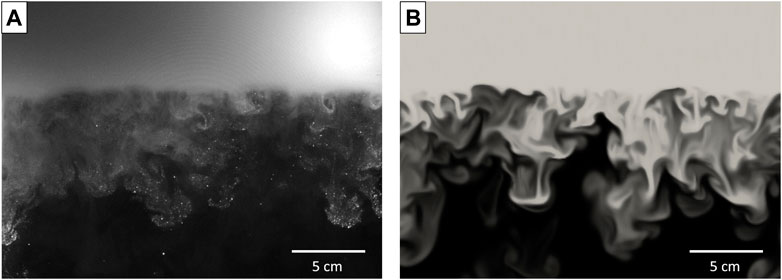
FIGURE 9. Settling-driven gravitational instabilities observed 19.5 s after the barrier removal (A) in the laboratory (Fries et al., 2021) and (B) in numerical simulations. Particle size: 40 µm and initial volume fraction: ${\varnothing }_0=2.78\times {10}^{-3}$.

Characterisation of the PBL and Effect of the Initial Particle Volume Fraction on the Finger Velocity

The bulk density profile ${\rho }_{\text{blk}}$, derived from the contributions of the particle concentration and sugar profiles, is given everywhere by the relation

${\mathit{\rho }}_{\mathit{blk}}=\varnothing {\mathit{\rho }}_{\mathit{p}}+\left(1-\varnothing \right){\mathit{\rho }}_{\mathit{f}}.(47)$

Figure 10 shows the profiles of $\varnothing$, ${\rho }_f$ and ${\rho }_{\text{blk}}$ in the numerical simulations as well as in the experiments 8 s after the barrier removal for the same initial conditions (${\varnothing }_0=3.18\times {10}^{-3}$ ). Despite some differences associated with limitations in achieving idealised initial conditions in the experiments, as well as the experimental data collection method, it can be seen that, in both the model and the experiments, there is an increase of the bulk density below the initial interface, owing to the particle front moving downwards. This zone of excess density corresponds to the unstable PBL from which instabilities occur, generating fingers. To calculate the finger velocity using the same method as in experiments, we extract slices from the 3D numerical domain and manually track the fronts of several fingers (6–15 fingers) from when they become fully developed until just before they become too diluted (the duration of this phase is $\sim 5 s$). For each simulation with different volume fraction, we then average the velocity of all tracked fingers and the uncertainty is the standard deviation associated with each set of fingers used for the measurements. Figure 11A shows the average finger velocity $V_f$ as a function of ${\varnothing }_0$, for both experiments (Fries et al., 2021) and simulations. Our simulation results are in good agreement with the experimental measurements and highlight that the increase of $V_f$ with ${\varnothing }_0$ is non-linear.

FIGURE 10

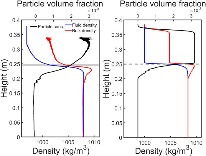
FIGURE 10. Density profile after 8 s for experiments (left) (Fries et al., 2021) and simulations (right) with ${\varnothing }_0=$ $3.18\times {10}^{-3}$ and a particle size of 40 µm. For clarity, the uncertainty on the experimental fluid density are not displayed on the figure and correspond to 0.8 kg m⁻³.

FIGURE 11

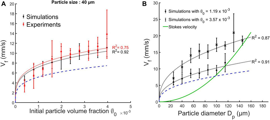
FIGURE 11. (A) Average finger speed (V_f) as a function of the initial volume fraction (${\varnothing }_0$) for a particle diameter of 40 μm. Red and black dotted lines show the best fits to the experiments (Fries et al., 2021) and simulations, respectively, using Eq. 1 with $G{r}_c$ as the fit parameter. For the simulations, we find $G{r}_c=1.2\pm 0.4\times {10}^4$ whilst for the experiments $G{r}_c=1.9\pm 0.7\times {10}^4$. (B) Average finger speed (V_f) as a function of the initial particle diameter (D_p), for two different particle volume fractions. The green line is the Stokes velocity for individual particles. The black dotted lines show the best fits to the simulations using Eq. 1 with $G{r}_c$ as the fit parameter. For ${\varnothing }_0=1.19\times {10}^{-3}$, the best fit gives $G{r}_c=7.6\times {10}^3$ and no fingers are observed to form for particle sizes higher than 115 µm. For ${\varnothing }_0=3.57\times {10}^{-3}$, the best fit gives $G{r}_c=2.7\times {10}^4$ and no fingers are observed to form for particle sizes higher than 145 µm. In the two plots, the blue dashed line shows Eq. 1 using $G{r}_c={10}^3$ from the analogy with thermal convection (Hoyal et al., 1999).

By analogy with thermal convection, it has previously been assumed that $G{r}_c={10}^3$ (Hoyal et al., 1999), but this is only an order of magnitude estimate and its application to settling-driven gravitational instabilities remains uncertain (Fries et al., 2021). Figure 11A shows good agreement between the simulations and Eq. 1 for a fitted $G{r}_c$ of $1.2\pm 0.4\times {10}^4$ ($R^2=0.92$), which is an order of magnitude higher than the value previously assumed (Hoyal et al., 1999; Carazzo and Jellinek, 2012). This agrees reasonably with the experiments, where the best fit is obtained for $G{r}_c=1.9\pm 0.7\times {10}^4$ ($R^2=0.75$), but the experimental results show more scatter. However, neither of these fits have completely satisfactory values of $R^2$. We therefore further investigate the applicability of Eq. 1 by examining the dependence of $V_f$ on ${\varnothing }_0$, assuming a more general power law of the form $V_f\propto {\varnothing }_0^q$. According to Eq. 1, $q=4/15\cong 0.27$. However, from the experiments, we obtain $q=0.50\pm 0.16$ (with $R^2=0.95$) while for our simulations $q=0.37\pm 0.08$ (with $R^2=0.98$). Here $G{r}_c$, $q$ and their associated uncertainties have been calculated accounting for the uncertainty on $V_f$ with the SciPy (Python-based ecosystem) procedure scipy. optimize.curve_fit.

Effect of Particle Size on the Finger Vertical Velocity

Since gravitational instabilities cause particles to sediment faster than their settling velocity, it is of interest to explore the transition from collective to individual settling, since this has implications for which grain sizes may prematurely sediment from a volcanic cloud (Scollo et al., 2017). Figure 11B shows the effect of particle size on the finger velocity as measured from the model, for two different initial volume fractions, in the experiments configuration (i.e., in the tank filled with water). We clearly observe two regimes:

• For particle sizes less than or equal to 115 µm (for ${\varnothing }_0=1.19\times {10}^{-3}$) and 145 µm (for ${\varnothing }_0=3.57\times {10}^{-3}$), we observe fingers, with the finger velocity increasing with particle size.

• For greater particle sizes, no fingers are observed to form.

From our simulations, we constrain the transition between the two regimes to occur at a critical particle diameter around 115 and 145 µm respectively for ${\varnothing }_0=1.19\times {10}^{-3}$ and ${\varnothing }_0=3.57\times {10}^{-3}$. We also note that this size range corresponds to the particle size at which the Stokes velocity exceeds the predicted finger velocity. This result agrees with the experimental observations of Scollo et al. (2017), who observed that no fingers form for particles with diameter larger than ∼125 µm with an initial particle volume fraction of ${\varnothing }_0=1.19\times {10}^{-3}$. We also compare the dependence of $V_f$ on the particle diameter with that predicted by Eq. 1 and find a best fit for $G{r}_c=7.6\pm 3.6\times {10}^3$ (with $R^2=0.91$) and $G{r}_c=2.7\pm 0.8\times {10}^4$ (with $R^2=0.87$) respectively for the two initial volume fractions (Figure 11B). We observe again that the values for the fitted $G{r}_c$ are greater than the one proposed by Hoyal et al. (1999) by analogy with thermal convection, whilst they also substantially differ from one another. We therefore also fit the results to a power law $V_f\propto D{p}^{\eta }$ finding $\eta =0.38\pm 0.13$ ($R^2=0.94$) and $\eta =0.42\pm 0.10$ ($R^2=0.88$) respectively to the two volume fractions which is in very good agreement with the analytical formulation (Eq. 1) that suggests $\eta =0.4$.

Particle Mass Flux, Particle Concentration in the Lower Layer and Accumulation Rate

Given the excellent agreement between the proposed model and both LSA analysis and analogue experiments described above, we take advantage of having 3D data from the numerical simulations in order to extract other parameters which are difficult to obtain otherwise (Fries et al., 2021). Three interesting parameters are the particle mass flux across a plane, the particle concentration in the lower layer and the amount of particles accumulated at the bottom of the tank, which can be related to the accumulation rate. The latter is especially interesting as, when the model is applied to volcanic clouds, it could eventually be compared with field data (Bonadonna et al., 2011).

We calculate the mass flux across a horizontal plane (actually a thin box of thickness $\delta x$) as shown in Figure 12A with

$J=\frac{\Delta m}{A\Delta t},(48)$

where $\Delta m$ is the mass crossing the yellow plane of area $A$ in time $\Delta t$, and is given by the mass difference in the volume below the plane between $t$ and $t-\Delta t$. The mass below at each time is calculated by summing the mass of particles in each cell $i$ of volume $\Delta V$, which is individually given by $m_i=\Delta V{\varnothing }_i{\rho }_p$. Figure 12B shows the temporal evolution of the particle mass flux settling through the yellow plane (located at 0.15 m below the barrier), for several initial particle volume fractions. The vertical black dashed line indicates the theoretical time $T_i$ when particles would be expected to reach the plane if they were settling individually at their Stokes velocity. For the different simulations, we clearly observe that the moments when the flux starts initially increasing (i.e., the arrival of the fastest finger) are much earlier than $T_i$ and this shows the extent to which the collective settling enhances the premature sedimentation. After the initial increase, the fluxes exhibit strong oscillations around a high plateau. These oscillations are associated with the intermittent nature of PBL detachment and the strong convection generated by fingers in the lower layer. Indeed, we observe that as soon as fingers reach the bottom of the tank, convection cells appear re-entraining some particles upward. The results show the net downward flux of particles and when particles are entrained upward, this consequently decreases the flux value. Interestingly, the different peaks show that we have some oscillatory convection and not steady convection. Finally, the particle mass flux reaches a plateau after some time which shows the end of convection and a transition to individual settling. Throughout, the average mass flux, as well as the amplitude of the oscillations increases with the initial volume fraction.

FIGURE 12

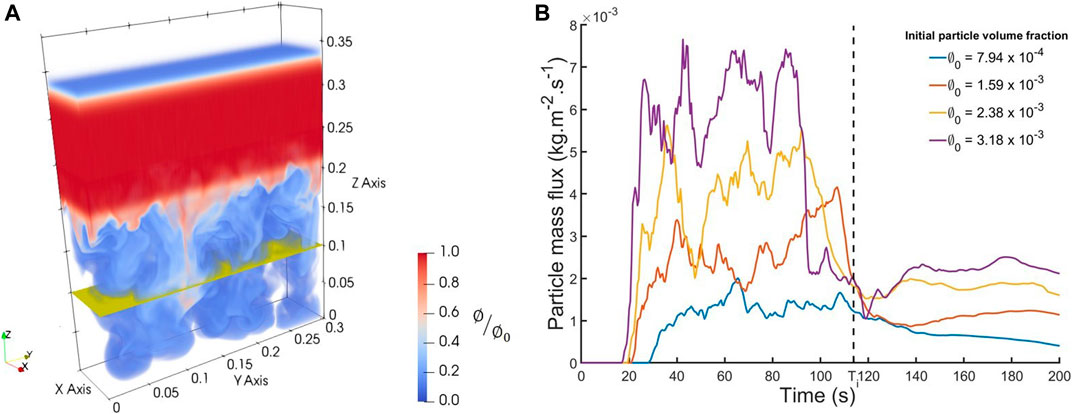
FIGURE 12. (A) Horizontal planar surface (yellow slice) located 0.15 m below the barrier, across which the particle mass flux is computed in the simulation domain. (B) Temporal evolution for the particle mass flux crossing the plane. Black dashed line: theoretical time for the particles to reach the plane at their individual Stokes velocity.

Another way to highlight the enhancement of the sedimentation rate by collective settling is to study the spatial distribution of particles beneath the interface. Assuming a quiescent upper layer and a convective lower layer, akin to our simulations, Hoyal et al. (1999) derived Eq. 4 for the evolution of the particle concentration in the lower layer. The derivation of this formulation assumes that ${\dot{M}}_{out}\ne 0$ since $t=0$ but in fact, ${\dot{M}}_{out}=0$ for $t<t_a$ where $t_a$ is the time when the first particles reach the bottom of the tank. Also, Eq. 4 only remains valid for $t<t_{lim}$, where $t_{lim}=h_1/V_s$, $h_1$ being the height of the upper layer. After this time, there are no longer any particles remaining in the upper layer and ${\dot{M}}_{in}=0$. We therefore propose an extension for the solution of the problem (see section 2.1 in Supplementary Material) which becomes

$C_2\left(t\right)=\frac{V_s}{h_2}{C}_1\left(0\right)t, \text{for} t<t_a,(49)$

$C_2\left(t\right)=C_1\left(0\right)\left[1+\left(\frac{V_s}{h_2}{t}_a-1\right)e^{-\frac{V_s}{h_2}\left(t-t_a\right)}\right], \text{for} t_a\le t<t_{lim},(50)$

$C_2\left(t\right)=C_1\left(0\right)\left[1+\left(\frac{V_{\mathit{s}}}{h_2}{t}_{\mathit{a}}-1\right)e^{-\frac{{\mathit{V}}_{\mathit{s}}}{{\mathit{h}}_2}\left({\mathit{t}}_{\mathit{lim}}-{\mathit{t}}_{\mathit{a}}\right)}\right]\left(1+\frac{h_1}{h_2}-\frac{V_{\mathit{s}}}{h_2}t\right),\text{for}t\ge t_{\lim },(51)$

where $h_2$ is the thickness of the lower layer. Equation 51 assumes that the convection stops at $t_{lim}$, which suggests a quiescent settling in the lower layer after that time with a constant flux ${\dot{M}}_{out}=A{V}_s{C}_2\left(t_{lim}\right)$.

An interesting result coming out of the previous analytical study is the mass of particles accumulating at the bottom of the tank and the associated accumulation rate. We can derive an analytical prediction for the mass of particles $m_b$ accumulated at the bottom of the tank for the different regimes highlighted above. Thus, by integration of the flux (see Section 2.2 in Supplementary Material) we have

$m_b=0, \text{for} t<t_a,(52)$

$m_b=m_0\frac{V_s}{h_1}\left[t+\left(\frac{h_2}{V_s}-t_a\right)e^{-\frac{V_s}{h_2}\left(t-t_a\right)}-\frac{h_2}{V_s}\right], \text{for} t_a\le t<t_{lim},(53)$

$m_b=m_0\frac{V_s}{h_1}\left\{t_{lim}-\frac{h_2}{V_s}\left[1+\left(\frac{V_s}{h_2}{t}_a-1\right)e^{-\frac{V_s}{h_2}\left(t_{lim}-t_a\right)}\right]\left(1+\frac{h_1}{h_2}-\frac{V_s}{h_2}t\right)\right\}, \text{for} t\ge t_{lim},(54)$

where $m_0$ is the initial mass of particles injected in the upper layer. Finally, at the time $t_{lim}+h_2/V_s$, all the particles have settled through the lower layer, thus $m_b=m_0$. Figure 13A shows the simulated particle accumulation at the bottom of the tank through time, for different particle sizes as well as the analytical prediction (Eqs 52–54). We compare as well with the analytical formulation of the mass which assumes that the lower is still turbulently convective even after the time $t_{lim}$ (Eq. S43 in Supplementary Material, dashed lines in Figure 13A). In order to compare between this prediction and the model results, $t_a$ is fitted in order to have the best agreement between the numerical data and Eqs 52–54. The results show clearly that the quiescent model of the lower layer for $t\ge t_{lim}$ agrees very well with the simulations and suggest that the entirely convective model underestimates the accumulation rate. Additionally, the fitted parameter $t_a$ is coherent with the time for the first fingers to reach the bottom of the tank in the simulations. Figure 13B shows the instantaneous accumulation rate computed from the numerical data for several initial volume fractions, as estimated by

$\frac{1}{A}\frac{d{m}_b}{dt},(55)$

FIGURE 13

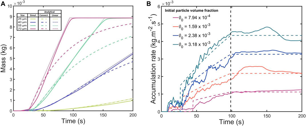
FIGURE 13. (A) Temporal evolution of the mass of particles accumulating at the bottom of the tank for several particle sizes. The dashed and dotted lines represent the extended analytical model of (Hoyal et al., 1999). Particle volume fraction ${\varnothing }_0=1.19\times {10}^{-3}$. (B) Accumulation rate calculated at the bottom of the tank for several particle volume fractions and a particle size of 40 µm. The coloured dashed lines are the rate derived from the analytical model. The black dashed line is the theoretical time at which all particles have settled across the interface.

We observe, for each initial particle volume fraction, an initial increase of the accumulation rate with time which reflects the enhancement of the sedimentation process due to convection. Interestingly, the accumulation rate then reaches a plateau at around $t=t_{lim}$, indicating that the system switches to a steady settling regime once all particles have left the upper layer. We compare also with the analytical relations which again have very good agreement with our simulations.

Finally, using the determined $t_a$, we can also calculate the concentration $C_2\left(t\right)$, as calculated with the analytical expressions in Eqs 49–51. Figure 14 shows a comparison with the average $C_2\left(t\right)$ as measured in simulations for a particle size of $40\text{μm}$ and three different initial upper layer concentrations, finding very good agreement.

FIGURE 14

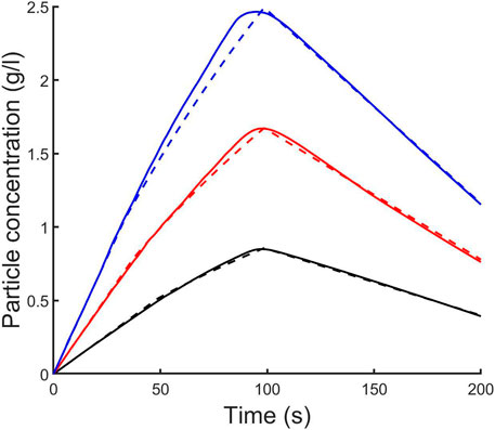
FIGURE 14. Evolution of the average particle volume fraction in the lower layer for particle of size 40 µm. Black: $C_0$ = 2 g/L (${\varnothing }_0=$ $7.94\times {10}^{-4}$), Red: $C_0$ = 4 g/L ($1.59\times {10}^{-3}$) and Blue: $C_0$ = 6 g/L ($2.38\times {10}^{-3}$). Solid lines: numerical model. Dashed lines: modified (Hoyal et al., 1999) model (Eqs 49–51).

Discussion

Model Caveats

Our numerical model has been validated by comparing various outputs with results from linear stability analysis, lab experiments (Fries et al., 2021) and theoretical predictions from previous studies (Hoyal et al., 1999; Carazzo and Jellinek, 2012). Even though these comparisons are good (Figures 9–14), the results provided by the model inherits the caveats of the experiments. Indeed, the static and confined configuration, as well as the fact that we performed the simulations in water, mean that we cannot fully extend the results to the volcanic case yet. Thus, further investigations are necessary to better simulate the volcanic environment (e.g., in air, with wind, etc.). Additionally, it is necessary to consider the limits of validity of the different assumptions. In our study, particles are small enough that they have no inertia and thus the fluid-particle interaction force is governed by the buoyant force term in the fluid momentum equation. However, as soon as the particle size increases, we need to consider some other dynamics. Indeed, a rigid particle moving in a fluid produces locally a disturbance flow which generates other contributions to the fluid-particle force terms. The assumption that particles settle at their Stokes velocity will then no longer be valid as the created local flow affects $V_S$ (Maxey and Riley, 1983; Cartwright et al., 2010; Patočka et al., 2020).

Whilst the condition on the particle coupling is given by the Stokes number ($St<1$), there is also a condition on the particle volume fraction to take in account. Harada et al. (2013) and Yamamoto et al. (2015) derived a dimensionless number in order to characterise the transition between fluid-like and particle-like settling. Although this number is only valid for narrow channel configurations, which are considerably different from ours, it highlights the fact that the particle size, volume fraction and characteristic length scale of the flow are critical parameters to define the validity of the continuum assumption. Thus, the transition from fluid-like to particle-like behaviour is achieved by decreasing the volume fraction and characteristic length scale and increasing the particle size. Near this transition, the use of a single-phase model, such as that presented here, should be treated with caution and this reveals the need for a comparison with future models which explicitly account for the drag contribution of individual particles. In multiphase models this contribution has been commonly represented through a force term involving the ratio between the phases differential velocities and the relaxation time (drag timescale) (Laibe and Price, 2014; Chou and Shao, 2016).

Another related caveat concerns the numerical diffusion underlying the use of an Eulerian approach to describe the transport of particles. Compared to classical first order finite difference methods, the use of the third order WENO procedure has drastically reduced the numerical diffusion. It is also possible to further reduce the induced numerical diffusion by increasing the order of the WENO scheme (i.e. increase also the computational cost). However, for problems purely related to advection, where the presence of any diffusion is critical, another strategy, such as two-phase models (using a Lagrangian approach where individual particles are explicitly modelled), has to be considered.

Vertical Finger Velocity

We have compared the simulated vertical velocity of fingers with experimental observations (Fries et al., 2021) and a theoretical prediction (Eq. 1) from (Hoyal et al., 1999; Carazzo and Jellinek, 2012) (Figure 11). This expression depends on a critical Grashof number, which by analogy with thermal convection (Turner, 1973) has previously been assumed to be 10³ (Hoyal et al., 1999). This value effectively corresponds to a dimensionless critical PBL thickness at which point the PBL can detach and form fingers. However, both the model results and experimental observations summarised in Figure 11 suggest that $G{r}_c>{10}^3$ for our configuration. Furthermore, as seen in Figure 11B, the curve for $V_f$ using $G{r}_c={10}^3$ (blue dotted line) crosses the Stokes velocity curve around $95 \text{μm}$ for instance with an initial particle volume fraction of ${\varnothing }_0=1.19\times {10}^{-3}$, suggesting this value should be the upper particle size limit for finger formation. However, in agreement with experiments (Scollo et al., 2017; Fries et al., 2021), we observe a larger threshold for the finger formation to be in the size range $[115-125] \text{μm}$, for ${\varnothing }_0=1.19\times {10}^{-3}$, and in the range $[145-160] \text{μm}$ for ${\varnothing }_0=3.57\times {10}^{-3}$, in this particular configuration. We also showed that Eq. 1 poorly predicts the observed dependence of the finger velocity on the initial particle volume fraction. Indeed, our studies suggests an alternative power law that better describes the dependence of $V_f$ on ${\varnothing }_0$. Equation 1 has been derived by a scaling theory that involves ${\delta }_{PBL}$ as characteristic length of the problem (Hoyal et al., 1999; Carazzo and Jellinek, 2012) and the discrepancies highlighted in this paper (Figure 11) may suggest that ${\delta }_{PBL}$ actually has a slightly different dependence on the initial particle volume fraction. Moreover, the use of the Grashof number as an appropriate scaling for the PBL thickness remains uncertain. On the one hand, our results suggest that if instability does occur once a critical Grashof number is reached, the critical value taken from the thermal convection analogy is not valid. On the other hand, the Grashof number may simply not be the correct dimensionless form of the PBL thickness, and different flow configurations will produce different critical values. The fact that both the experiments and simulations agree very well shows that the “true” value for $G{r}_c$, if it exists, is an order of magnitude higher than in the thermal case. However, Figure 11B shows that we find a ratio of $\sim 3.5$ between the two fitted $G{r}_c$ which is interestingly close to the ratio of three between the two associated particle volume fractions. Whilst the variability of $G{r}_c$ might come from the measurement itself (fitting of the numerical and experimental data), this behaviour is coherent considering the definition of $G{r}_c$ (ratio between buoyancy and viscous forces) and the fact that the buoyancy force is a function of the particle volume fraction. Obviously, this is only the case so long as the particle concentration does not affect the bulk viscosity, which is the case in our study. Therefore, we highlight here that the order of magnitude found for $G{r}_c$ is valid for the flow configuration presented in this study and also that there is a dependence on the initial particle volume fraction. Further analyses with different flow configurations (i.e., different buoyancy and viscous conditions) are required to constrain the variability of $G{r}_c$ and confirm that it may not be a rigorous scaling for the PBL thickness. A study involving settling-driven gravitational instabilities in air and in the presence of shear is currently performed and will certainly provide some insights on the dependence of $G{r}_c$ on the flow configuration.

The predicted dependence of the finger velocity on the particle diameter by Eq. 1 shows a very good agreement with our simulated results, as confirmed by a power-law fitting between $V_f$ and $D_p$. Thus, whilst we have demonstrated the need for a better scaling of ${\delta }_{PBL}$, Eq. 1 can still provide a good estimate for the particle size threshold to form fingers. Consequently, if the size threshold to form fingers is given when Eq. 1 equals the Stokes velocity (Eq. 13) we can derive a formulation for the threshold

$D_p^{\ast }={\left[\frac{{\left(18\mu \right)}^2\varnothing {\delta }_{PBL}}{g\left({\rho }_p-{\rho }_f\right){\rho }_f}\sqrt{\left(\frac{\pi }{4}\right)}\right]}^{\frac{1}{4}}.(56)$

The main caveats for this formulation are that it strongly depends on having a correct scaling for ${\delta }_{PBL}$ and obviously this estimation is valid under the assumption that particles settle at their Stokes velocity, which is reasonable for our study but might be uncertain in nature where the ambient fluid is air and for non-spherical particles.

Particle Concentration in the Lower Layer and Mass Accumulation Rate

We have proposed a modified analytical formulation for the particle concentration in the lower layer $C_2\left(t\right)$ and consequently for the mass of particles accumulated at the bottom of the tank $m_b\left(t\right)$. Despite some numerical artefacts that can be seen on Figure 13B where the computed accumulation rate seems to be non-zero before $t_a$, there is very good agreement between the simulations and the analytical model. The artefacts themselves are due to fluctuating numerical errors that do not affect the final results.

The analytical predictions for $C_2\left(t\right)$ and $m_b\left(t\right)$ are step-wise functions depending on $t_a$, the time it takes for the first particles to reach the bottom. For $t<t_a$, the analytical model predicts that $C_2\left(t\right)$ increases linearly with time since the formulation assumes that, during this period, particles are settling individually. In fact, our numerical results show that convective settling does occur for $t<t_a$ but, since this time period is short, the linear law seems to be a satisfactory approximation for the early-time average lower layer particle concentration. However, in order to compare our simulated results with the analytical prediction, we fitted the parameter $t_a$ in this study. Although we are able to obtain excellent agreement between model and theory, it would be better to develop a fully independent formulation. To achieve this, it is necessary to also provide an analytical estimation for $t_a$. One possible approach would be to assume the decomposition $t_a=t_a^{\prime }+t_a^{″}$ where $t_a^{\prime }$ is the time during which the PBL initially grows beneath the interface at the individual particle settling velocity, i.e., $t_a^{\prime }={\delta }_{PBL}/V_s$, and $t_a^{″}$ is the time between the PBL detachment and the first arrival of particles at the base of the domain. If, during this stage, we assume that the particles are advected at the finger velocity then $t_a^{″}=\left(h_2-{\delta }_{PBL}\right)/V_f$). We therefore see that $t_a$ strongly depends on ${\delta }_{PBL}$, which highlights once again the need for a correct scaling of the PBL thickness, as discussed in the previous section.

Another interesting result concerns the accumulation rate of particles at the base of the domain in the presence of fingers. Figure 13B shows the accumulation rate increases with time for $t_a<t<t_{lim}$, in agreement with the analytical prediction (i.e., combination of Eqs 53, 55 which provides an exponential increase of $m_b$). Conversely, if the particles had settled individually, the accumulation rate would be temporally constant. However, there is no denying that the effect as a function of position is also interesting in order to characterise especially the consequences of the oscillatory convection on the sedimentation rate. We computed an animated map (Supplementary Material) showing the spatial distribution of the sedimentation rate at the tank floor through time, for an initial particle volume fraction of $1.98\times {10}^{-3}$. As expected, the convection in the lower layer initiated by fingers generates a spatially inhomogeneous sedimentation rate which strongly evolves in time. Furthermore, we also observe that the temporal evolution stops a time around the theoretical time when we expect all particle have left the upper layer (i.e., end of convection). Generally, all these aspects show that temporally resolved measurements of the accumulation rate of particles from volcanic clouds may record temporal signatures of sedimentation via settling-driven gravitational instabilities. Whilst there is already a spatial deposit signature of settling-driven gravitational instabilities (i.e. bimodal grainsize distribution) (Bonadonna et al., 2011; Manzella et al., 2015), this is not unique and can be generated by other mechanisms such as particle aggregation (Brown et al., 2012). Accumulation rate data from the field may therefore provide a powerful tool for distinguishing the efficiency of convective sedimentation beneath volcanic clouds.

Conclusion

We have presented an innovative hybrid Lattice Boltzmann-Finite Difference 3D model in order to simulate settling-driven gravitational instabilities at the base of volcanic ash clouds. Such instabilities occur when particles settle through a density interface at the base of a suspension, leading to the formation of an unstable particle boundary layer (Hoyal et al., 1999; Carazzo and Jellinek, 2012; Manzella et al., 2015), and also occur in other natural settings, such as river plumes (Davarpanah Jazi and Wells, 2016). Our numerical model makes use of a low-diffusive WENO procedure to solve the advection-diffusion-settling equation for the particle volume fraction. The use of such a routine allows us to minimise errors associated with numerical diffusion and has the advantage of being applied to simple uniform meshes, which makes the coupling with the LBM easier. This innovative use of the WENO scheme, therefore, represents an effective tool for the solving of advection-dominated problems. Our implementation of the third order WENO finite difference scheme will be integrated in a future release of the open-source Palabos code. Our model has been successfully validated by comparing the results with 1) predictions from linear stability analysis where we show that the model is able to simulate settling-driven gravitational instabilities from the initial disturbance through the linearly-unstable regime, 2) analogue experiments (Fries et al., 2021) and 3) theoretical models (Hoyal et al., 1999; Carazzo and Jellinek, 2012) in order to reproduce the non-linear regime which describes the downward propagation of fingers. We also confirmed the premature sedimentation process through collective settling compared to individual settling.

Our model provides new insights into:

• The value of the critical Grashof number. From measurements of the vertical finger speed, we have found $G{r}_c\sim {10}^4$ in our configuration. This value differs from the one suggested by analogy with thermal convection ($G{r}_c\sim {10}^3$) (Hoyal et al., 1999). Our results suggest that either the critical Grashof number for settling-driven gravitational instabilities is greater than in the thermal convection case or that the Grashof number may not be the correct dimensionless form of the PBL thickness. In any case, this highlights the need for further investigation of the scaling of the PBL thickness ${\delta }_{PBL}$.

• The presence of a particle size threshold for the finger formation. Using our results, we have proposed an analytical formulation for this threshold depending on the density of particles, the viscosity of the medium and also the bulk density difference between the two fluid layers.

• The signature of settling-driven gravitational instabilities (i.e., accumulation rate). We show that the accumulation rate of particles at the tank base initially increases with time before reaching a plateau. This contrasts with the constant accumulation rate associated with individual particle settling. This suggests that accumulation rate data could be used during tephra fallout to distinguish between sedimentation through settling-driven gravitational instabilities and individual-particle sedimentation.

We have also demonstrated how our numerical model can be used to expand the initial conditions and configuration settings that can be explored through experimental investigations. The results presented so far in an aqueous media permitted model validation but have also opened fundamental questions that will be addressed in future works involving configurations more similar to the natural system. Indeed, thanks to the strengths of the LBM, the model can easily be applied to more complex systems and provides a robust tool for the transition from the laboratory studies to volcanic systems, as well as other environmental flows.

Data Availability Statement

The raw data supporting the conclusions of this article will be made available by the authors, without undue reservation.

Author Contributions

JL integrated the WENO procedure in the Palabos framework, conducted the simulations and data analysis under the supervision of PJ, JLä, CB, and BC. JL drafted the manuscript. JLä and BC were involved in the development of the Palabos code. All authors have contributed to data interpretation as well as the editing and finalising of the paper.

Funding

The study has been funded by the Swiss National Science Foundation #200021_169463.

Conflict of Interest

The authors declare that the research was conducted in the absence of any commercial or financial relationships that could be construed as a potential conflict of interest.

Publisher’s Note

All claims expressed in this article are solely those of the authors and do not necessarily represent those of their affiliated organizations, or those of the publisher, the editors and the reviewers. Any product that may be evaluated in this article, or claim that may be made by its manufacturer, is not guaranteed or endorsed by the publisher.

Acknowledgments

All the simulations presented in this paper have been performed using the High Performance Computing (HPC) facilities Baobab and Yggdrasil of the University of Geneva. We would like to thank Amanda B. Clarke and Jeremy C. Phillips for constructive discussions. The authors are grateful to SS, TM, BA and the Editor for their constructive reviews. A preprint of this work has been submitted on the arXiv server in the Fluid Dynamics category on the June 14, 2021: arXiv:2106.07694 (Lemus et al., 2021).

Supplementary Material

The Supplementary Material for this article can be found online at: https://www.frontiersin.org/articles/10.3389/feart.2021.713175/full#supplementary-material.

References

Alsinan, A., Meiburg, E., and Garaud, P. (2017). A Settling-Driven Instability in Two-Component, Stably Stratified Fluids. J. Fluid Mech. 816, 243–267. doi:10.1017/jfm.2017.94

CrossRef Full Text | Google Scholar

Bagnato, E., Aiuppa, A., Bertagnini, A., Bonadonna, C., Cioni, R., Pistolesi, M., et al. (2013). Scavenging of sulphur, Halogens and Trace Metals by Volcanic Ash: The 2010 Eyjafjallajökull Eruption. Geochimica et Cosmochimica Acta 103, 138–160. doi:10.1016/j.gca.2012.10.048

CrossRef Full Text | Google Scholar

Baltensperger, R., and Berrut, J.-P. (2001). The Linear Rational Collocation Method. J. Comput. Appl. Math. 134, 243–258. doi:10.1016/s0377-0427(00)00552-5

CrossRef Full Text | Google Scholar

Berrut, J.-P., and Mittelmann, H. D. (2004). Adaptive point Shifts in Rational Approximation with Optimized Denominator. J. Comput. Appl. Math. 164-165, 81–92. doi:10.1016/S0377-0427(03)00485-0

CrossRef Full Text | Google Scholar

Bhatnagar, P. L., Gross, E. P., and Krook, M. (1954). A Model for Collision Processes in Gases. Phys. Rev. 94, 515–525. doi:10.1103/physrev.94.511

CrossRef Full Text | Google Scholar

Blong, R. (2000). “Volcanic Hazards and Risk Management,” in Encyclopedia of Volcanoes (Cambridge: Academic Press), 1215–1227.

Google Scholar

Bonadonna, C., Biass, S., Menoni, S., and Gregg, C. E. (2021). Assessment of Risk Associated with Tephra-Related Hazards. Forecasting and Planning for Volcanic Hazards, Risks, and Disasters 2, 329–378. doi:10.1016/b978-0-12-818082-2.00008-1

CrossRef Full Text | Google Scholar

Bonadonna, C., Folch, A., Loughlin, S., and Puempel, H. (2012). Future Developments in Modelling and Monitoring of Volcanic Ash Clouds: Outcomes from the First IAVCEI-WMO Workshop on Ash Dispersal Forecast and Civil Aviation. Bull. Volcanol. 74, 1–10. doi:10.1007/s00445-011-0508-6

CrossRef Full Text | Google Scholar

Bonadonna, C., Genco, R., Gouhier, M., Pistolesi, M., Cioni, R., Alfano, F., et al. (2011). Tephra Sedimentation during the 2010 Eyjafjallajökull Eruption (Iceland) from deposit, Radar, and Satellite Observations. J. Geophys. Res. 116. doi:10.1029/2011JB008462

CrossRef Full Text | Google Scholar

Brown, R. J., Bonadonna, C., and Durant, A. J. (2012). A Review of Volcanic Ash Aggregation. Phys. Chem. Earth 45–46, 67–78. doi:10.1016/j.pce.2011.11.001

PubMed Abstract | CrossRef Full Text | Google Scholar

Burgisser, A., Bergantz, G. W., and Breidenthal, R. E. R. (2005). Addressing Complexity in Laboratory Experiments: The Scaling of Dilute Multiphase Flows in Magmatic Systems. J. Volcanology Geothermal Res. 141, 245–265. doi:10.1016/j.jvolgeores.2004.11.001

CrossRef Full Text | Google Scholar

Burns, P., and Meiburg, E. (2012). Sediment-laden Fresh Water above Salt Water: Linear Stability Analysis. J. Fluid Mech. 691, 279–314. doi:10.1017/jfm.2011.474

CrossRef Full Text | Google Scholar

Burns, P., and Meiburg, E. (2014). Sediment-laden Fresh Water above Salt Water: Nonlinear Simulations. J. Fluid Mech. 762, 156–195. doi:10.1017/jfm.2014.645

CrossRef Full Text | Google Scholar

Carazzo, G., and Jellinek, A. M. (2012). A New View of the Dynamics, Stability and Longevity of Volcanic Clouds. Earth Planet. Sci. Lett. 325-326, 39–51. doi:10.1016/j.epsl.2012.01.025

CrossRef Full Text | Google Scholar

Cardoso, S. S. S., and Zarrebini, M. (2001). Convection Driven by Particle Settling Surrounding a Turbulent Plume. Chem. Eng. Sci. 56, 3365–3375. doi:10.1016/S0009-2509(01)00028-8

CrossRef Full Text | Google Scholar

Carey, S. (1997). Influence of Convective Sedimentation on the Formation of Widespread Tephra Fall Layers in the Deep Sea. Geol 25, 839–842. doi:10.1130/0091-7613(1997)025<0839:iocsot>2.3.co;2

CrossRef Full Text | Google Scholar

Cartwright, J. H. E., Feudel, U., Károlyi, G., De Moura, A., Piro, O., and Tél, T. (2010). Dynamics of Finite-Size Particles in Chaotic Fluid Flows. Nonlinear Dynamics and Chaos: Advances and Perspectives 51(1), 87. doi:10.1007/978-3-642-04629-2_4

CrossRef Full Text | Google Scholar

Chandrasekhar, S. (1961). Hydrodynamic and Hydromagnetic Stability. Oxford: Oxford University Press.

Google Scholar

Chou, Y.-J., and Shao, Y.-C. (2016). Numerical Study of Particle-Induced Rayleigh-Taylor Instability: Effects of Particle Settling and Entrainment. Phys. Fluids 28, 043302. doi:10.1063/1.4945652

CrossRef Full Text | Google Scholar

Costa, A., Folch, A., and Macedonio, G. (2010). A Model for Wet Aggregation of Ash Particles in Volcanic Plumes and Clouds: 1. Theoretical Formulation. J. Geophys. Res. 115, 1–14. doi:10.1029/2009JB007175

CrossRef Full Text | Google Scholar

Crimaldi, J. P. (2008). Planar Laser Induced Fluorescence in Aqueous Flows. Exp. Fluids 44, 851–863. doi:10.1007/s00348-008-0496-2

CrossRef Full Text | Google Scholar

Davarpanah Jazi, S., and Wells, M. G. (2016). Enhanced Sedimentation beneath Particle-Laden Flows in Lakes and the Ocean Due to Double-Diffusive Convection. Geophys. Res. Lett. 43, 10,883–10,890. doi:10.1002/2016GL069547

CrossRef Full Text | Google Scholar

Durant, A. J. (2015). RESEARCH FOCUS: Toward a Realistic Formulation of fine-ash Lifetime in Volcanic Clouds. Geology 43, 271–272. doi:10.1130/focus032015.1

CrossRef Full Text | Google Scholar

Folch, A. (2012). A Review of Tephra Transport and Dispersal Models: Evolution, Current Status, and Future Perspectives. J. Volcanology Geothermal Res. 235-236, 96–115. doi:10.1016/j.jvolgeores.2012.05.020

CrossRef Full Text | Google Scholar

Folch, A., Mingari, L., Gutierrez, N., Hanzich, M., Macedonio, G., and Costa, A. (2020). FALL3D-8.0: A Computational Model for Atmospheric Transport and Deposition of Particles, Aerosols and Radionuclides - Part 1: Model Physics and Numerics. Geosci. Model. Dev. 13, 1431–1458. doi:10.5194/gmd-13-1431-2020

CrossRef Full Text | Google Scholar

Fries, A., Lemus, J., Jarvis, P. A., Clarke, A. B., Phillips, J. C., Manzella, I., et al. (2021). The Influence of Particle Concentration on the Formation of Settling-Driven Gravitational Instabilities at the Base of Volcanic Clouds. Front. Earth Sci. 9. doi:10.3389/feart.2021.640090

CrossRef Full Text | Google Scholar

Godunov (1959). A Difference Scheme for Numerical Solution of Discontinuous Solution of Hydrodynamic Equations. Math. Sb. 47, 271–306.

Google Scholar

Godunov (1954). Different Methods for Shock Waves. Moscow, Russia: Moscow State Univ.

Google Scholar

Gouhier, M., Eychenne, J., Azzaoui, N., Guillin, A., Deslandes, M., Poret, M., et al. (2019). Low Efficiency of Large Volcanic Eruptions in Transporting Very fine Ash into the Atmosphere. Sci. Rep. 9, 1–12. doi:10.1038/s41598-019-42489-z

PubMed Abstract | CrossRef Full Text | Google Scholar

Gudmundsson, G. (2011). Respiratory Health Effects of Volcanic Ash with Special Reference to Iceland. A Review. Clin. Respir. J. 5, 2–9. doi:10.1111/j.1752-699X.2010.00231.x

PubMed Abstract | CrossRef Full Text | Google Scholar

Guffanti, M., Mayberry, G. C., Casadevall, T. J., and Wunderman, R. (2008). Volcanic Hazards to Airports. Nat. Hazards 51, 287–302. doi:10.1007/s11069-008-9254-2

CrossRef Full Text | Google Scholar

Guo, Z., Zheng, C., and Shi, B. (2002). Discrete Lattice Effects on the Forcing Term in the Lattice Boltzmann Method. Phys. Rev. E 65, 1–6. doi:10.1103/PhysRevE.65.046308

PubMed Abstract | CrossRef Full Text | Google Scholar

Harada, S., Kondo, M., Watanabe, K., Shiotani, T., and Sato, K. (2013). Collective Settling of fine Particles in a Narrow Channel with Arbitrary Cross-Section. Chem. Eng. Sci. 93, 307–312. doi:10.1016/j.ces.2013.01.054

CrossRef Full Text | Google Scholar

He, X., and Luo, L.-S. (1997). Theory of the Lattice Boltzmann Method: From the Boltzmann Equation to the Lattice Boltzmann Equation. Phys. Rev. E 56, 6811–6817. doi:10.1103/PhysRevE.56.6811

CrossRef Full Text | Google Scholar

Hosseini, S. A., Darabiha, N., Thévenin, D., and Eshghinejadfard, A. (2017). Stability Limits of the Single Relaxation-Time Advection-Diffusion Lattice Boltzmann Scheme. Int. J. Mod. Phys. C 28, 1750141. doi:10.1142/S0129183117501418

CrossRef Full Text | Google Scholar

Hoyal, D. C. J. D., Bursik, M. I., and Atkinson, J. F. (1999). Settling-driven Convection: A Mechanism of Sedimentation from Stratified Fluids. J. Geophys. Res. 104, 7953–7966. doi:10.1029/1998jc900065

CrossRef Full Text | Google Scholar

Jacobs, C. T., Collins, G. S., Piggott, M. D., Kramer, S. C., and Wilson, C. R. G. (2013). Multiphase Flow Modelling of Volcanic Ash Particle Settling in Water Using Adaptive Unstructured Meshes. Geophys. J. Int. 192, 647–665. doi:10.1093/gji/ggs059

CrossRef Full Text | Google Scholar

Jenkins, S. F., Wilson, T. M., Magill, C., Miller, V., Stewart, C., Blong, R., et al. (2015). Volcanic Ash Fall hazard and Risk. Global Volcanic Hazards and Risk, 173–222. doi:10.1017/CBO9781316276273.005

CrossRef Full Text | Google Scholar

Jiang, G.-S., and Shu, C.-W. (1996). Efficient Implementation of Weighted ENO Schemes. J. Comput. Phys. 126, 202–228. doi:10.1006/jcph.1996.0130

CrossRef Full Text | Google Scholar

Jones, A., Thomson, D., Hort, M., and Devenish, B. (2007). The U.K. Met Office's Next-Generation Atmospheric Dispersion Model, NAME III. Air Pollut. Model. Its Appl. XVII 1, 580–589. doi:10.1007/978-0-387-68854-1_62

CrossRef Full Text | Google Scholar

Keck, J.-B., Cottet, G.-H., Meiburg, E., Mortazavi, I., and Picard, C. (2021). Double-diffusive Sedimentation at High Schmidt Numbers: Semi-lagrangian Simulations. Phys. Rev. Fluids 6, 1–10. doi:10.1103/PhysRevFluids.6.L022301

CrossRef Full Text | Google Scholar

Koochesfahani, M. M. (1984). Experiments on Turbulent Mixing and Chemical Reactions in a Liquid Mixing Layer. Journal of Fluid Mechanics. doi:10.7907/Y7BR-C556

CrossRef Full Text | Google Scholar

Kruger, T., Kusumaatmaja, H., Kuzmin, A., Shardt, O., Goncalo, S., and Viggen, E. M. (2017). The Lattice Boltzmann Method. Principles and Practice 1. doi:10.1191/0265532206lt326oa

CrossRef Full Text | Google Scholar

Laibe, G., and Price, D. J. (2014). Dusty Gas with One Fluid. Mon. Not. R. Astron. Soc. 440, 2136–2146. doi:10.1093/mnras/stu355

CrossRef Full Text | Google Scholar

Latt, J., Malaspinas, O., Kontaxakis, D., Parmigiani, A., Lagrava, D., Brogi, F., et al. (2021). Palabos: Parallel Lattice Boltzmann Solver. Comput. Math. Appl. 81, 334–350. doi:10.1016/j.camwa.2020.03.022

CrossRef Full Text | Google Scholar

Leclaire, S., Parmigiani, A., Malaspinas, O., Chopard, B., and Latt, J. (2017). Generalized Three-Dimensional Lattice Boltzmann Color-Gradient Method for Immiscible Two-phase Pore-Scale Imbibition and Drainage in Porous media. Phys. Rev. E 95, 33306. doi:10.1103/PhysRevE.95.033306

PubMed Abstract | CrossRef Full Text | Google Scholar

Lemus, J., Fries, A., Jarvis, P. A., Bonadonna, C., Chopard, B., and Latt, J. (2021). Modelling Settling-Driven Gravitational Instabilities at the Base of Volcanic Clouds Using the Lattice Boltzmann Method. Available at: https://arxiv.org/abs/2106.07694.

CrossRef Full Text | Google Scholar

Lewis, D. J. (1950). The Instability of Liquid Surfaces when Accelerated in a Direction Perpendicular to Their Planes. II. Proc. R. Soc. Lond. A. 202, 81–96. doi:10.1098/rspa.1950.0086

CrossRef Full Text | Google Scholar

Liu, X.-D., Osher, S., and Chan, T. (1994). Weighted Essentially Non-oscillatory Schemes. J. Comput. Phys. 115(1), 1–32. doi:10.1006/jcph.1994.1187

CrossRef Full Text | Google Scholar

Manville, V., and Wilson, C. J. N. (2004). Vertical Density Currents: A Review of Their Potential Role in the Deposition and Interpretation of Deep-Sea Ash Layers. J. Geol. Soc. 161, 947–958. doi:10.1144/0016-764903-067

CrossRef Full Text | Google Scholar

Manzella, I., Bonadonna, C., Phillips, J. C., and Monnard, H. (2015). The Role of Gravitational Instabilities in Deposition of Volcanic Ash. Geology 43, 211–214. doi:10.1130/G36252.1

CrossRef Full Text | Google Scholar

Maters, E. C., Cimarelli, C., Casas, A. S., Dingwell, D. B., and Murray, B. J. (2020). Volcanic Ash Ice-Nucleating Activity Can Be Enhanced or Depressed by Ash-Gas Interaction in the Eruption Plume. Earth Planet. Sci. Lett. 551, 116587. doi:10.1016/j.epsl.2020.116587

CrossRef Full Text | Google Scholar

Maxey, M. R., and Riley, J. J. (1983). Equation of Motion for a Small Rigid Sphere in a Nonuniform Flow. Phys. Fluids 26, 883–889. doi:10.1063/1.864230

CrossRef Full Text | Google Scholar

Niemeier, U., Timmreck, C., Graf, H.-F., Kinne, S., Rast, S., Self, S., et al. (2009). Initial Fate of fine Ash and Sulfur from Large Volcanic Eruptions. Atmos. Chem. Phys. 9, 9043–9057. doi:10.5194/acp-9-9043-2009

CrossRef Full Text | Google Scholar

Noriega, H., Reggio, M., and Vasseur, P. (2013). Natural Convection of Nanofluids in a Square Cavity Heated from below. Comput. Therm. Sci. Int. J. 5. doi:10.1615/computthermalscien.2013006652

CrossRef Full Text | Google Scholar

Parmigiani, A., Huber, C., Chopard, B., Latt, J., and Bachmann, O. (2009). Application of the Multi Distribution Function Lattice Boltzmann Approach to thermal Flows. Eur. Phys. J. Spec. Top. 171, 37–43. doi:10.1140/epjst/e2009-01009-7

CrossRef Full Text | Google Scholar

Patočka, V., Calzavarini, E., and Tosi, N. (2020). Settling of Inertial Particles in Turbulent Rayleigh-Bénard Convection. Phys. Rev. Fluids 5, 1–36. doi:10.1103/PhysRevFluids.5.114304

CrossRef Full Text | Google Scholar

Prata, A. T., Mingari, L., Folch, A., Macedonio, G., and Costa, A. (2021). FALL3D-8.0: A Computational Model for Atmospheric Transport and Deposition of Particles, Aerosols and Radionuclides - Part 2: Model Validation. Geosci. Model. Dev. 14, 409–436. doi:10.5194/gmd-14-409-2021

CrossRef Full Text | Google Scholar

Prata, F., and Rose, B. (2015). Volcanic Ash Hazards to Aviation, ed. H. B. T.-T. E. of V. (Second E. Sigurdsson (Amsterdam: Academic Press), 911–934. doi:10.1016/B978-0-12-385938-9.00052-3

CrossRef Full Text | Google Scholar

Roche, O., and Carazzo, G. (2019). The Contribution of Experimental Volcanology to the Study of the Physics of Eruptive Processes, and Related Scaling Issues: A Review. J. Volcanology Geothermal Res. 384, 103–150. doi:10.1016/j.jvolgeores.2019.07.011

CrossRef Full Text | Google Scholar

Scollo, S., Bonadonna, C., and Manzella, I. (2017). Settling-driven Gravitational Instabilities Associated with Volcanic Clouds: New Insights from Experimental Investigations. Bull. Volcanol. 79, 1–14. doi:10.1007/s00445-017-1124-x

CrossRef Full Text | Google Scholar

Scollo, S., Folch, A., Coltelli, M., and Realmuto, V. J. (2010). Three-dimensional Volcanic Aerosol Dispersal: A Comparison between Multiangle Imaging Spectroradiometer (MISR) Data and Numerical Simulations. J. Geophys. Res. 115, 1–14. doi:10.1029/2009JD013162

CrossRef Full Text | Google Scholar

Scollo, S., Tarantola, S., Bonadonna, C., Coltelli, M., and Saltelli, A. (2008). Sensitivity Analysis and Uncertainty Estimation for Tephra Dispersal Models. J. Geophys. Res. Solid Earth 113, 1–17. doi:10.1029/2006jb004864

CrossRef Full Text | Google Scholar

Sharp, D. H. (1984). An Overview of Rayleigh-Taylor Instability. Physica D: Nonlinear Phenomena 12, 3–18. doi:10.1016/0167-2789(84)90510-4

CrossRef Full Text | Google Scholar

Spence, R. J. S., Kelman, I., Baxter, P. J., Zuccaro, G., and Petrazzuoli, S. (2005). Residential Building and Occupant Vulnerability to Tephra Fall. Nat. Hazards Earth Syst. Sci. 5, 477–494. doi:10.5194/nhess-5-477-2005

CrossRef Full Text | Google Scholar

Stenchikov, G., Ukhov, A., Osipov, S., Ahmadov, R., Grell, G., Cady‐Pereira, K., et al. (2021). How Does a Pinatubo‐Size Volcanic Cloud Reach the Middle Stratosphere. Geophys. Res. Atmos. 126. doi:10.1029/2020JD033829

CrossRef Full Text | Google Scholar

Stokes, G. G. (1851). On the Theories of the Internal Friction of Fluids in Motion, and of the Equilibrium and Motion of Elastic Solids. Math. Phys. Pap. 19, 75–129. doi:10.1017/CBO9780511702242.005

CrossRef Full Text | Google Scholar

Succi, S., Sbragaglia, M., and Ubertini, S. (2010). Lattice Boltzmann Method. Scholarpedia 5, 9507. doi:10.4249/scholarpedia.9507

CrossRef Full Text | Google Scholar

Turner, J. S. (1973, Buoyancy Effects in Fluids. Cambridge: Cambridge University Press. doi:10.1017/CBO9780511608827

CrossRef Full Text | Google Scholar

Völtz, C., Pesch, W., and Rehberg, I. (2001). Rayleigh-Taylor Instability in a Sedimenting Suspension. Phys. Rev. E 65, 011404. doi:10.1103/PhysRevE.65.011404

CrossRef Full Text | Google Scholar

Watt, S. F. L., Gilbert, J. S., Folch, A., Phillips, J. C., and Cai, X. M. (2015). An Example of Enhanced Tephra Deposition Driven by Topographically Induced Atmospheric Turbulence. Bull. Volcanol. 77, 35. doi:10.1007/s00445-015-0927-x

CrossRef Full Text | Google Scholar

Wilson, T. M., Cole, J. W., Stewart, C., Cronin, S. J., and Johnston, D. M. (2011). Ash Storms: Impacts of Wind-Remobilised Volcanic Ash on Rural Communities and Agriculture Following the 1991 Hudson Eruption, Southern Patagonia, Chile. Bull. Volcanol. 73, 223–239. doi:10.1007/s00445-010-0396-1

CrossRef Full Text | Google Scholar

Yamamoto, Y., Hisataka, F., and Harada, S. (2015). Numerical Simulation of Concentration Interface in Stratified Suspension: Continuum-Particle Transition. Int. J. Multiphase Flow 73, 71–79. doi:10.1016/j.ijmultiphaseflow.2015.03.007

CrossRef Full Text | Google Scholar

Yu, X., Hsu, T.-J., and Balachandar, S. (2014). Convective Instability in Sedimentation: 3-D Numerical Study. J. Geophys. Res. Ocean., 3868–3882. doi:10.1002/2014jc010123

CrossRef Full Text | Google Scholar

Yu, X., Hsu, T.-J., and Balachandar, S. (2013). Convective Instability in Sedimentation: Linear Stability Analysis. J. Geophys. Res. Oceans 118, 256–272. doi:10.1029/2012JC008255

CrossRef Full Text | Google Scholar

Zhu, Y., Toon, O. B., Jensen, E. J., Bardeen, C. G., Mills, M. J., Tolbert, M. A., et al. (2020). Persisting Volcanic Ash Particles Impact Stratospheric SO2 Lifetime and Aerosol Optical Properties. Nat. Commun. 11, 1–11. doi:10.1038/s41467-020-18352-5

PubMed Abstract | CrossRef Full Text | Google Scholar