A simulation study on the climatic responses to short-lived climate pollutants changes from the pre-industrial era to the present

1 Introduction

Carbon dioxide (CO₂) is the most important anthropogenic driver of global warming. Besides CO₂, Short-lived climate pollutants (SLCPs) have strong contributions to the warming, as well. SLCPs is a set of warming climate forcers, which are gases and particles that can affect the climate by modifying the global energy budget and influence human health. SLCPs includes methane (CH₄, a well-mixed greenhouse gas with warming effect second to CO₂), tropospheric ozone (O₃), and black carbon (BC). They have lifetimes in the atmosphere of a few days to a decade, shorter than the timescale for stabilizing the climate (Borgar et al., 2016). As important climate-forcing factors, SLCPs contribute to 40%–45% of total global warming (UNEP&WMO, 2011). Xie et al. (2016a), Xie et al. (2016b) found the increased CH₄ and tropospheric O₃ concentrations since pre-industrial times have resulted in a global annual mean surface air temperature (SAT) increase of 0.31 and 0.36°C, respectively. Removing all anthropogenic BC emissions would cause a global cooling of 0.05°C according to Stohl et al. (2015).

The short lifetimes of SLCPs cause spatially and temporally inhomogeneous distribution and concentrations tend to be highest nearer to source regions. Therefore, the resulting forcing patterns are also inhomogeneous, and the regional and global climatic responses is much more complex than to CO₂ (Shindell et al., 2009; Shindell and Faluvegi, 2009). For the majority of emissions of SLCPs are in the Northern Hemisphere (NH), so their forcing is prominent in the NH (Shindell, 2014). Borgar et al. (2017) found that SLCPs could significantly affect the potential for temperature change in the Arctic and mid latitudes of the Northern Hemisphere (NH). Meanwhile, the Arctic Monitoring and Assessment Programme (2015) assessed the effects of regional SLCPs emissions on the Arctic, indicating that non-CH₄ SLCPs emissions from East and South Asia had the greatest warming effect in the Arctic. Xie et al. (2016a), Xie et al. (2016b) found both CH₄ and tropospheric O₃ lead to more obvious warming in Northern Hemisphere. BC emissions in Europe and East Asia led to Arctic temperature response 390% and 240% larger than the global temperature response, respectively (Borgar et al., 2017). The warming in eastern China due to BC and tropospheric O₃ was 0.62°C and 0.43°C, respectively, much higher than their effects on globally averaged SAT (Chang et al., 2009).

IPCC AR6 indicates that rapid, effective and sustained reductions in emissions of SLCPs are essential to the goal of limiting near-term warming (IPCC, 2021; Sun et al., 2022). Lots of evidences suggest that reducing SLCPs would play a key role to prevent global warming from exceeding 1.5°C or 2°C above pre-industrial levels (Shindell and Smith, 2019; Harmsen et al., 2020). Zhang et al. (2018) evaluated the ERFs caused by changes in SLCPs concentrations from 2010 to 2050 under RCP8.5, RCP4.5, and RCP2.6, which were 0.1, −0.3, and −0.5 W m⁻², respectively. They also indicated that there would be a 0.57 K reduction in global warming by 2050 under strong SLCPs mitigation. Xu and Ramanathan (2017) obtained a consistent conclusion with Zhang et al. (2018), and suggested that reducing SLCPs would bring more benefits than abating CO₂ only (Xu and Ramanathan, 2017; Dreyfus et al., 2022). Specifically, quickly reducing the emissions of CH₄ and BC could avoid 0.3°C and 0.2°C of warming by 2050, respectively. Shindell et al. (2012) and Ramanathan and Xu (2010) reached similar conclusions. If the concentrations of all SLCPs were reduced using current technologies, the rise of sea surface level could be reduced by approximately 25% by 2050 (Hu et al., 2013) and 22%–42% by 2100 (Ramanathan and Xu, 2010).

Most of the existing scientific studies and public policies about SLCPs have focused mainly on single species of SLCPs or the possible influences on climate due to SLCPs changes in the future. In this study, we focus on how SLCPs have already affected our past global and regional climates and to what extent they did by comparing with the contribution from CO₂. In order to measure and compare the effects of different factors on global and regional SAT, we firstly need to evaluate quantitatively the driver of climatic change, effective radiative forcing (ERF), defined as the change of the net radiant flux at the TOA or the tropopause, after allowing for atmospheric temperatures, water vapour, clouds and land albedo to adjust, but with global surface temperature unchanged (Myhre et al., 2013; Smith et al., 2018). Xie et al. (2016a), Xie et al. (2016b) estimated the ERFs of CH₄ from 1750 to 2011 and tropospheric O₃ from 1850 to 2013 both to be 0.46 W m⁻² by using a global climate model combined with satellite observations. IPCC AR6 evaluated ERFs (from 1750 to 2019) of CH₄ and O₃ to be 0.54 ± 0.11 and 0.47 ± 0.23 W m⁻², respectively. However, quantitative assessment on ERF of overall SLCPs is very limited.

This study, the ERF of overall SLCPs is estimated by using an online aerosol–climate model (BCC_AGCM2.0_CUACE/Aero); then evaluate the global and reginal climate responses to SLCPs concentration changes from the year of 1850 to 2010 and estimate quantitatively what warming is resulted from the SLCPs compared with CO₂ in the past. The model, data sets, and methods used in this work are described in Section 2. The ERF and climate response due to changes in SLCPs concentrations and comparisons with those of CO₂ are presented in Section 3; Our conclusion are summarized in Section 4.

2 Data, model, and scheme description

2.1 Model

In this study, we used an online aerosol–climate model, BCC_AGCM2.0_CUACE/Aero, developed by Zhang et al. (2012b), Zhang et al. (2014) and Wang et al. (2014). The model incorporates the atmospheric general circulation model BCC_AGCM2.0, developed by the Beijing Climate Center of the China Meteorological Administration (BCC/CMA) and an aerosol model CUACE/Aero, developed by the Chinese Academy of Meteorological Sciences (CAMS). BCC_AGCM2.0 employs a horizontal T42 spectral resolution (about 2.8° × 2.8°) and a hybrid vertical coordinate with 26 levels, the top of which is located at about 2.9 hPa. The CUACE/Aero aerosol model (Gong et al., 2002, Gong et al., 2003) considers five types of aerosols (sulfate, black carbon, organic carbon, dust, and sea salt) and multiple aerosol physical and chemical processes (including anthropogenic aerosol emissions, gaseous chemistry, transport, coagulation, and removal), more detailed introduction of CUACE/Aero can be found in Zhang et al. (2016). BCC_AGCM2.0_CUACE/Aero reproduces fairly well the present-day climate at regional and global scales, especially for temperature and wind (Wu et al., 2008; Wu et al., 2010). The radiation scheme BCC_RAD (Zhang et al., 2014; Zhang, 2016) and the McICA cloud vertical overlap scheme (Jing and Zhang, 2012, Jing and Zhang, 2013; Zhang et al., 2014) are used in BCC_AGCM2.0. These improvements have reduced the error in the simulated longwave and shortwave radiative fluxes at the TOA and the surface compared to the original version. The model also includes physical representations of the aerosol direct, semi-direct, and indirect effects for liquid-phase clouds (Wang et al., 2014). BCC_AGCM2.0_CUACE/Aero reproduces fairly well the present-day climate at regional and global scales, especially for temperature and wind (Wu et al., 2008; Wu et al., 2010). This model simulates the atmospheric burden and geographical distribution of aerosols reasonably well (Zhang et al., 2012a; Wang et al., 2014), and is widely used in studies of aerosol and GHG RF estimations and their impacts on climate (Zhang et al., 2012a, Zhang et al., 2016, Zhang et al., 2018; Wang et al., 2013a, Wang et al., 2013b, Wang et al., 2015, Wang et al., 2016; Zhao et al., 2014; Xie et al., 2016a, Xie et al., 2016b). It was a member of AeroCom phase II comparisons of aerosol direct RF (Myhre et al., 2012) and organic aerosol modeling comparisons (Tsigaridis et al., 2014).

2.2 Data

The CO₂ and SLCPs data, including BC emissions and CO₂, tropospheric O₃, and CH₄ concentrations, were obtained from the representative concentration pathways (RCPs) in AR5. There are four concentration emission paths, RCP2.6, RCP4.5, RCP6.0, and RCP8.5, named for their projected RF values (unit: W m⁻²) in 2100. In this study, the emissions and concentrations of CO₂ and SLCPs in 1850 were obtained from historical projection and inventory data in the RCP Database (Mieville et al., 2010) and the current (2010) data were taken from RCP4.5 (Wise et al., 2009). Changes in the concentration of CO₂ and SLCPs from the year of 1850 to 2010 are shown in Section 3.1.

2.3 Experimental design

To calculate the ERFs caused by changes in the SLCPs and CO₂ concentrations from the year of 1850 to 2010, we performed three sets of experiments, consisting of two perturbing experiments (S_ERF2010 and C_ERF2010, the simulations with the changes from 1850 to 2010 in SLCPs and CO₂ concentration, respectively) and a control experiment (ERF₁₈₅₀, the simulation keep SLCPs and CO₂ concentration at 1850). The experimental configurations are given in Table 1. In this study, the method of “fixed-SST” was selected to estimate ERF (IPCC, 2021), which means that sea surface temperature and sea ice were kept constant during the above three sets of experiments. We ran 15 years in each simulation, of which the last 10 years of data were averaged to estimate the ERFs, as follows:

$\mathrm{E}\mathrm{R}\mathrm{F}\left(\mathrm{S}\mathrm{L}\mathrm{C}\mathrm{P}\mathrm{s}\right)=\mathrm{\Delta }{\mathrm{F}}_{\mathrm{S}\mathrm{E}\mathrm{R}\mathrm{F}2010}-\mathrm{\Delta }{\mathrm{F}}_{\mathrm{E}\mathrm{R}\mathrm{F}1850}$

$\mathrm{E}\mathrm{R}\mathrm{F}\left(\mathrm{C}{\mathrm{O}}_2\right)=\mathrm{\Delta }{\mathrm{F}}_{\mathrm{C}\mathrm{E}\mathrm{R}\mathrm{F}2010}-\mathrm{\Delta }{\mathrm{F}}_{\mathrm{E}\mathrm{R}\mathrm{F}1850}$

where ∆F was the net radiation flux (the difference between incoming and outgoing radiative flux, both shortwave and longwave) at the top of the model (for there is little difference in net radiation flux between the top of the model and the TOA). The ∆F_SERF2010, ∆F_CERF2010, and ∆F_ERF1850 are the net radiation flux of S_ERF2010, C_ERF2010, and ERF₁₈₅₀, respectively.

TABLE 1

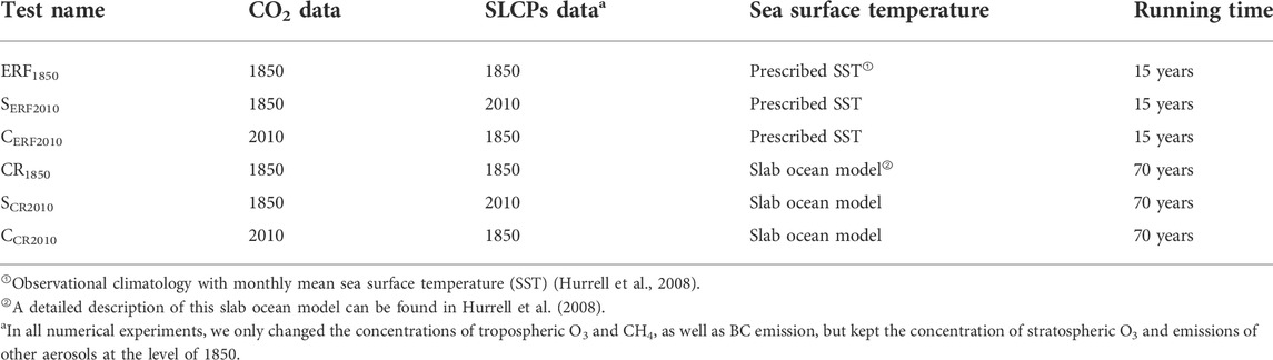
TABLE 1. Experimental design.

Another three sets of numerical experiments (S_{CR 2010}, C_{CR 2010}, and CR ₁₈₅₀) were performed to simulate climate responses to changes in SLCPs and CO₂ concentrations, using the model coupled with a slab ocean model (Hurrell et al., 2008). We evaluated the SLCPs- and CO₂-induced climate responses (CR), as follows:

$\mathrm{C}\mathrm{R}\left(\mathrm{S}\mathrm{L}\mathrm{C}\mathrm{P}\mathrm{s}\right)={\mathrm{S}}_{\mathrm{C}\mathrm{R}2010}-{\mathrm{C}\mathrm{R}}_{1850}$

${\mathrm{C}\mathrm{R}(\mathrm{C}\mathrm{O}}_2{)=\mathrm{C}}_{\mathrm{C}\mathrm{R}2010}{-\mathrm{C}\mathrm{R}}_{1850}$

To allow the global mean SAT to reach a quasi-equilibrium state, the coupled model requires an adjustment of 30 years (Kristjánsson et al., 2005); therefore, we ran 70 years in the three simulation tests, and results for the last 40 years were used for the analysis.

The t-test was used on the ERF and climate responses to estimate their statistical significance in this study. The t-test is the test for a difference between two sample means, as follows:

$t=\frac{\overline{X_1}-\overline{X_2}}{\sqrt{\frac{\left(n_1-1\right)S_1^2+\left(n_2-1\right)S_2^2}{n_1+n_2-2}}\left(\frac{1}{n_1}+\frac{1}{n_2}\right)}$

Where X and S is the average and variance of the sample, and n is sample size. The confidence coefficient of 95% was chosen in this study, which means that ERF (climate responses) will pass the significance test when its absolute t-value is greater than 2.262 (2.045).

3 Results

3.1 Changes in the concentration of CO₂ and SLCPs from the year of 1850 to 2010

Since the Industrial Revolution, the emissions of CO₂ and SLCPs and their concentration in the atmosphere have increased remarkably due to the development of human activities. Based on the input data of CO₂, CH₄, and ozone concentrations used in this study (mentioned in Section 2.2), by 2010, the global annual average CO₂ and CH₄ concentration has increased by 118 ppm and 942 ppb, relative to 1850. As shown in Figures 1B,D, tropospheric ozone column concentrations generally increase by more than 12 DU in middle and high latitudes in the Northern Hemisphere, with two increasing centers in Bohai and Mediterranean regions, which is consistent with the results of An et al. (2022). According to our simulations (as shown in Figures 1A,C), the annual mean column concentrations of BC increased more than 0.4 mg m⁻² in Eastern China, Northern India, and Central Africa, of which up to 1.6 mg m⁻² in Eastern China.

FIGURE 1

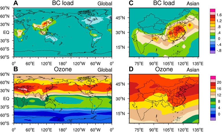
FIGURE 1. Annual mean differences of BC loading (top, unit: mg m⁻²) between S_ERF2010 and ERF₁₈₅₀, and tropospheric ozone changes from the year of 1850 to 2014 (bottom, unit: DU).

3.2 ERF of SLCPs in 2010, relative to 1850

Figure 2 shows the distributions of ERF of SLCPs in 2010, relative to 1850. SLCPs concentrations have increased significantly since the pre-industrial era, which produced notably positive ERFs over most parts of the globe, especially in the Ural Mountains region, the southern Indian Ocean, East Asia, the central Pacific, and most parts of the Atlantic. The ERFs were greater than 1.5 W m⁻² over above-mentioned areas, and the largest positive ERFs occurred over central and eastern China (CEC), with the value more than 4.0 W m⁻². According to the definition of ERF (see Section 2.3), the spatial distribution of ERF depends on many factors, such as changes in SLCPs concentrations and adjustment of clouds and other factors. The notably positive ERFs over continents were mainly from shortwave ERFs (similar to ERF, but for the change of the net shortwave radiant flux). For instance, over the Ural Mountains region and CEC, shortwave ERFs were more than 2.0 W m⁻², and longwave ERFs (similar to ERF, but for the change of the net longwave radiant flux) were approximately 0 W m⁻² (Figures 2B,C). The decrease in low cloud cover (LCC: above 680 hPa) of about 1.2%–2.0% resulted in less solar radiation being scattered, and induced strong positive ERFs over the Ural Mountains region and CEC (Figures 3B,E).

FIGURE 2

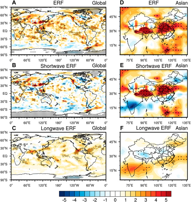
FIGURE 2. Annual mean ERF (top), shortwave ERF (middle), and longwave ERF (bottom), which are obtained by the difference between S_ERF2010 and ERF₁₈₅₀, unit: W m⁻². The areas with “⋅” passed the 95% significance test.

FIGURE 3

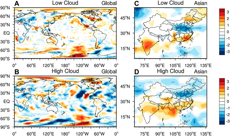
FIGURE 3. Annual mean differences of low cloud (top) and high cloud (bottom) between S_ERF2010 and ERF₁₈₅₀, unit: %.

The BC loadings in the CEC has increased by about 1.4 mg m⁻² (see Figure 1C) since the pre-industrial era, which has also led to positive shortwave ERF there. The BC loading has also increased in India, but the shortwave ERF was about −3.5 W m⁻² there (Figure 2E), which was mainly attributed to the increased LCC (about 1.8%) scattering more solar radiation. The positive ERFs over the ocean were caused by both shortwave and longwave ERFs. The increased SLCPs concentrations led to the longwave ERFs being about 1.0 W m⁻² over most parts of the ocean (Figure 2C), and the shortwave ERFs over the middle of the Indian Ocean, North of the Equatorial Pacific, and the North Atlantic Ocean being 0.5–1.0 W m⁻². Notably, over the East and West of the Gulf of Mexico, and the sea area of southern Japan, longwave ERFs were over 2.0 W m⁻² due to increased high cloud cover (HCC: below 440 hPa) (Figure 3B) by absorbing thermal radiation.

Due to the short atmospheric lifetimes of SLCPs, the spatial pattern of SLCPs ERF is more inhomogeneous than CO₂ ERF. There are more human activities in NH than in Southern Hemisphere (SH), leading to greater SLCPs emissions; therefore, the ERF of NH was 1.24 [0.97–1.51] W m⁻² larger than that of SH [about 0.75 (0.47–1.04) W m⁻²]. Meanwhile, the CO₂ ERF during 1850–2010 in the NH and SH were both 1.50 [1.35–1.65] W m⁻². The global annual mean ERFs were 0.99 [0.79–1.20] and 1.50 [1.35–1.65] W m⁻² due to the changes in SLCPs and CO₂ concentrations since pre-industrial era, respectively. Therefore, the SLCPs ERF was equivalent to 66%, 83%, and 50% of the CO₂ ERF in global, NH, and SH terms, respectively. Previous studies had indicated that ERF is virtually identical to RF for CO₂ and CH₄ (Hansen et al., 2005). By comparison (shown in Table 2), the ERF of this study was consistent with these results.

TABLE 2

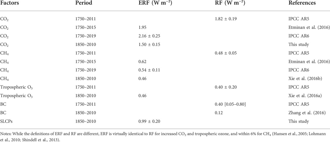
TABLE 2. Comparison of ERFs in this work and the simulated ERFs/RFs from other studies due to changes in variety of greenhouse gases and BC since the pre-industrial era (Units: W m⁻²).

3.3 Temperature response to changes in SLCP concentrations

The increases in SLCPs concentrations since the pre-industrial era have produced positive ERF and warming effect in most parts of the globe. As shown in Figure 5, SAT increased by over 1.0 K (past 95% significance test) in North America, most of Europe, the Arctic region, northwestern China, and the ribbon area near 60°S. The changes in SAT are consistent with that of surface net radiation flux (SNRF), which composed of shortwave (the surface net solar flux, abbreviated to FSNS) and longwave (the surface net longwave flux, abbreviated to FSNS) components. As shown in Figures 4A,D, the SNRF increased by more than 2.5 W m⁻² in the above-mentioned regions. The SNRF is substantially affected by changes in SLCPs concentrations, clouds, and surface albedo. In northeastern China, increases in CH₄ and O₃ concentrations leaded to FLNS increase by about 2.0 W m⁻² (Figure 4F), while FSNS decrease by 2.0 W m⁻² (Figure 4E), and eventually caused a weak increase in SAT (Figure 5B) there. These might be due to the 1.2% increase of LCC (Figure 6D) reflecting more solar radiation, which blocked a part of the shortwave radiation reaching the surface, and weakened the warming effect of SLCPs in northeastern China. Sea ice cover near the Antarctic decreased by about 10% (figure not shown), causing a decrease in surface albedo, which decreased the reflection of solar radiation around Antarctic and led to FSNS increases of about 3.5 W m⁻². This series of processes ultimately resulted in the SAT increasing by approximately 1.5 K in the Antarctic. The FLNS increased across most of the globe, particularly in middle and lower latitudes (Figure 4C). This was due to significant increases in CH₄ and O₃ concentrations (Xie et al., 2016a, Xie et al., 2016b). Changes in cloud cover, especially middle and high clouds, also can influence the FLNS. In northern Africa, the decrease in HCC of more than 2.5% (Figure 6C) produced a decrease of FLNS by 0.5 W m⁻² due to more outgoing longwave radiation, and ultimately offset part of the warming effect caused by SLCPs there. In western America, reduced middle cloud cover (Figure 6B) resulted in a 1.5 W m⁻² decrease in the FLNS, whereas simultaneously the reduced LCC increased the FSNS by about 3.5 W m⁻² by reflecting less downward solar radiation. The opposite changes of FLNS and FSNS eventually resulted in notable increases in SNRF and SAT in western America.

FIGURE 4

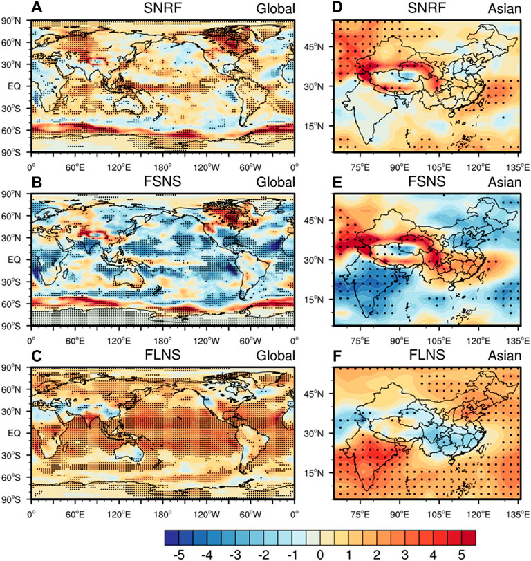
FIGURE 4. Annual mean differences of SNRF (top), FSNS (middle), and shortwave FLNS (bottom) between S_CR2010 and CR₁₈₅₀, unit: W m⁻². The areas with “⋅” passed the 95% significance test.

FIGURE 5

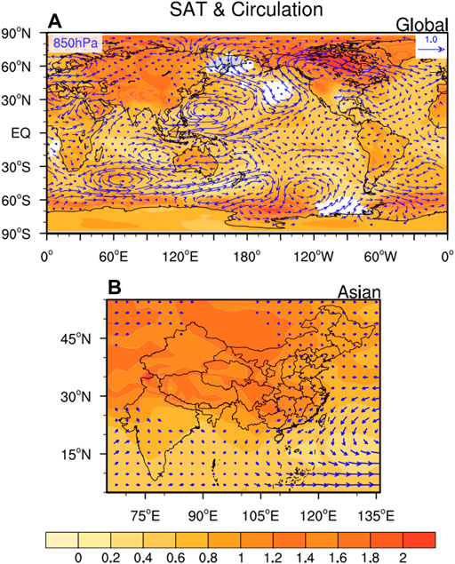
FIGURE 5. Annual mean differences of surface air temperature (contour, unit: K) and 850 hPa circulation (vector) between S_CR2010 and CR₁₈₅₀. The areas without color did not pass the 95% significance test.

FIGURE 6

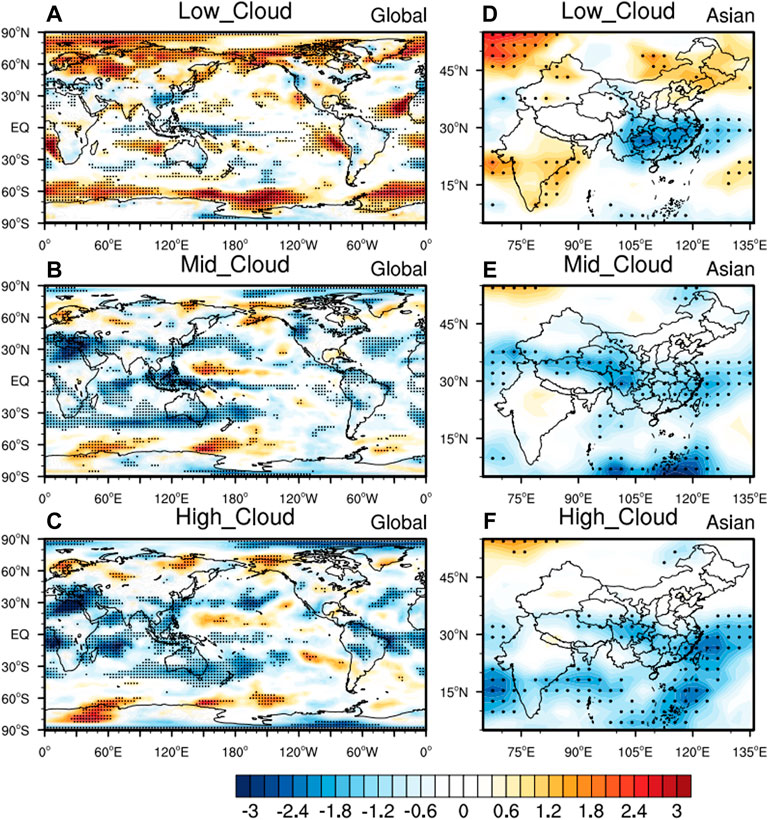
FIGURE 6. Annual mean differences of low (top), middle (middle), and high (bottom) cloud covers between S_CR2010 and CR ₁₈₅₀, unit: %. The areas with “⋅” passed the 95% significance test.

The concentrations of SLCPs have increased significantly in both southern China and the Indian Peninsula since the pre-industrial era (Xu et al., 2021), but the warming in China was much greater (Figure 5B). This was mainly due to the contrasting patterns of cloud changes in these two regions, as discussed in Section 3.3. The 1.5% decrease in LCC (Figure 6D) led to 1.5 W m⁻² increase in the FSNS in southern China (Figure 4E). Conversely, in the Indian Peninsula, the LCC increased about 1%, and resulted in a decrease in the FSNS of 3.5 W m⁻². Although the changes in the FLNS were the opposite of those in the FSNS in these two regions, thus, the increase in the SNRF in southern China were greater than it in the Indian Peninsula, which ultimately increase SAT in southern China and the Indian Peninsula by 0.9 and 0.3 K, respectively.

From the year of 1850 to 2010, changes in CO₂ concentrations caused significant increases in the SAT in high latitudes of the NH, northwestern China, and the ribbon area near 60°S (Supplementary Figure S1). The CO₂-induced average warmings in global, NH, and SH were 1.62 [1.48–1.76], 1.67 [1.50–1.83], and 1.58 [1.43–1.73] K, respectively. The distribution of SAT changes induced by CO₂ was similar to that caused by SLCPs. The changes in SLCPs led to global, NH, and SH average temperature increases of 0.70 [0.60–0.80], 0.78 [0.62–0.94], and 0.62 [0.45–0.74] K, respectively, which were equivalent to 43% of the CO₂-induced warmings. In China, SLCPs concentrations (especially BC) increased remarkably, this resulted in the SLCPs-induced warming in this region equivalent to 55% of the CO₂-induced.

3.4 Cloud cover response to changes in SLCP concentrations

Changes in SLCPs concentrations from 1850 to 2010 had little effect on global average cloud cover, but a large effect on regional cloud cover. As shown in Figure 6A, the increasing centers of LCC were mainly located over high latitudes of the NH, the ocean around Antarctica, and near the equator (especially over the east Pacific and Atlantic). Over central Africa, the Indian Peninsula, and most of the United States, where the surface relative humidity (SRH) increased by about 1.5% (Figure 8C), LCC increased by 1.0%, which indicates LCC have a good correlation between relative humidity (Chris, 1994). However, circulation is also an influential factor in cloud. In mid-India, where the change in SRH was weak, for example, the 2% increase in LCC was mainly due to enhanced cyclonic vorticity. Conversely, enhanced anticyclonic vorticity in the southern Pacific led to a 1.0% decrease in LCC. In high latitudes of the SH, LCC increased by more than 2%, which was largely due to the increases in relative humidity and enhanced updrafts between 900 and 700 hPa over 60°S (Figures 7A,B). SLCPs concentrations have increased significantly in both the Indian Peninsula and southern China since the pre-industrial era; however, there were opposite changes in the LCC over these two regions. LCC increased by about 1.0% over the Indian Peninsula but decreased by about 1.8% over southern China (Figure 6D), mainly due to the 1.5% and −1.4% changes in SRH in these two areas, respectively (Figure 8F). The geographical distributions of changes in middle cloud cover and HCC were similar (Figures 6B,C). HCC clearly decreased over northern Africa, the Indian Ocean, the northern and southern Pacific, and the equatorial Atlantic, especially over northern Africa and the Indian Ocean with decreases of about 2.2%–3.0%. This was caused by a reduction in the relative humidity of about 1.3% between 400 and 200 hPa over the subtropics (Figure 7B). Over the high latitudes in both the NH and SH (near 60°S and 60°N), HCC increased by about 1.5% due to increases in relative humidity below 300 hPa.

FIGURE 7

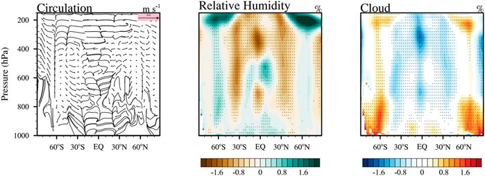
FIGURE 7. Annual mean differences in zonally averaged circulation (left column), relative humidity (middle column), and cloud fraction (right column) between S_CR2010 and CR₁₈₅₀. The areas with “⋅” passed the 95% significance test.

FIGURE 8

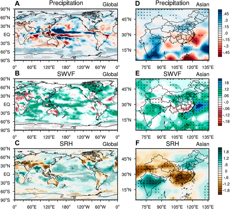
FIGURE 8. Annual mean differences of precipitation (top, unit: mm d⁻¹), SWVF (middle, unit: kg m⁻²d⁻¹), and SRH (bottom, unit:%) between S_CR2010 and CR₁₈₅₀. The areas with “⋅” passed the 95% significance test.

3.5 Precipitation response to changes in SLCP concentrations

Figure 8 shows the changes in precipitation (left column), surface water vapor flux (SWVF) (middle column), and SRH (right column) caused by the increased SLCPs concentrations. Changes in SLCPs concentrations produced significant increases in the SWVF (around 0.10 kg m⁻² day⁻¹) over most marine areas, especially the equatorial Pacific, Central Indian Basin, and East China Sea (Figure 8B). The most significant increase (over 0.18 kg m⁻² day⁻¹) occurred over the East China Sea. Decreases in the SWVF were mainly apparent over most continents and were caused by the reductions in the SNRF. In northern Africa, southern Europe, Australia, and most parts of South America, the SNRF decreased by about 1.0 W m⁻², leading to a reduction of about 0.10 kg m⁻² day⁻¹ in the SWVF. The changes in the SWVF had a great influence on the changes in SRH. In the most parts of the Pacific and northern Atlantic, SRH increased by 0.6% due to the increases in the SWVF. Conversely, with reductions in the SWVF, SRH decreased by 0.8% in northern Africa, Australia, and most parts of South America. Changes in circulation also affected the local SRH. For example, in eastern Canada, the SWVF increased by 0.10 kg m⁻² day⁻¹, but the SRH decreased due to enhanced flows from inland. It is worth noting that the opposite changes in SRH occurred in the Indian Peninsula and southern China. As shown in Figure 8F, in the Indian Peninsula, the increased SWVF with the enhanced cross-equatorial flows caused a 1.5% increase in SRH. However, in southern China, the enhanced flow, from land to ocean, blocked water vapor transport in the South Asian Monsoon, with a SWVF reduction of 0.06 kg m⁻² day⁻¹; thus, SRH ultimately decreased by 1.8% there. As shown in Figure 8A, precipitation mainly increased (about 0.10 mm d⁻¹) in mid-high latitudes and decreased (about −0.20 mm d⁻¹) in subtropical regions. In tropical areas, precipitation increased significantly in the NH and decreased in the SH. The largest changes in precipitation occurred in the north and south of the Pacific equatorial region, with the maximum increase (decrease) of 0.50 mm d⁻¹ (−0.45 mm d⁻¹). According to a simulation by Broccoli et al. (2006), the interhemispheric asymmetry in SAT changes led to the movement of the Intertropical Convergence Zone (ITCZ) toward the relatively warmer hemisphere. In our simulation, the change in the annual mean SAT was +0.9 K in the NH and +0.6 K in the SH, and there was a northward shift of the ITCZ, which was the opposite of the trends induced by anthropogenic aerosols (e.g., Zhang et al., 2016; Zhou et al., 2018). Since the pre-industrial era, changes in SLCPs concentrations have caused global mean precipitation to increase by 0.03 mm d⁻¹ (approximately 0.6%). Therefore, our simulation results indicate that the global mean precipitation has increased by about 1.0% per K surface temperature in response to SLCPs forcing, which is lower than the result (1.5–2% K⁻¹) obtained by Salzmann (2016).

4 Conclusion

We simulated the ERF and climate responses to changes in SLCPs concentrations from 1850 to the present (represented by the model year of 2010) using an aerosol–climate coupled model of BCC_AGCM2.0_CUACE/Aero. The global annual mean ERF due to changes in SLCPs concentrations since the pre-industrial era was 0.99 W m⁻². The largest positive ERF was more than 4.0 W m⁻², and occurred over central and eastern China, mainly due to adjustments in low cloud cover and BC loading. The greater level of human activity in NH led to more SLCPs emissions than in SH, and correspondingly the SLCPs ERF in NH is larger than that in SH. We found that the SLCPs ERF was equivalent to 66%, 83%, and 50% of the CO₂ ERF in global, NH, and SH terms, respectively. Increased SLCPs concentrations led to warming effects over most parts of the globe, with obvious warming in the mid-high latitudes of NH and the ocean around Antarctica, where increases reached 1.0 K. Precipitation increased by about 0.10 mm d⁻¹ in mid-high latitudes and was reduced by about 0.20 mm d⁻¹ in subtropical regions. As a result of the interhemispheric asymmetry in SAT changes caused by SLCP, ITCZ moved toward NH. Changes in SLCPs concentrations caused increases in the global annual mean SAT and precipitation of 0.70 K and 0.02 mm d⁻¹, respectively. In our simulation, the global mean precipitation increased by about 1.0% per K surface warming in response to the forcing by SLCPs. From the year of 1850 to 2010, the increase in SAT caused by SLCPs was equivalent to 43% of the warming effect of CO₂ over the globe and 55% over China. Increased SLCPs concentrations had little effect on global average cloud cover, but had obvious effects on regional cloud cover. Low cloud cover increased by about 2.5% over high latitudes in the NH and the ribbon area near 60°S, whereas high cloud cover increased more than 2.0% over northern Africa and the Indian Ocean.

SLCPs concentrations have increased significantly in both the Indian Peninsula and southern China since the pre-industrial era; however, the respective relative humidity at the surface of the two regions changed by 1.5% and −1.8%, and low cloud cover by 1.0% and −1.8%, with the opposite signs. The enhanced cross-equatorial flows and a weakened South Asian Monsoon maybe important driving factors for these opposite changes over these two regions. Combining the direct effect of SLCPs and the consequent cloud response, the final SAT increases were 0.3 K in the Indian Peninsula and 0.9 K in southern China.

Our results suggest that SLCPs-induced warming should not be underestimated, which was equivalent to half of the global warming effect of CO₂, even much larger in the regions with more coal consuming (e.g., China). SLCPs can influence regional SAT by affecting radiation budget; while the circulation response to SLCPs change in driving the changes of regional SAT is also important.

Data availability statement

The datasets presented in this study can be found in online repositories. The names of the repository/repositories and accession number(s) can be found below: All simulation results, we analysed in this article, can be found by https://data.mendeley.com/datasets/k6j57m9g46/draft?a=3305cd05-7d4e-46f8-8c30-330d8211b5e6.

Author contributions

BX made the whole calculations and analyses of this work, wrote the first draft. HZ gave the idea of this work and substantially revised the manuscript. All authors read and approved the final manuscript.

Funding

This work was financially supported by the National Key R&D Program of China (2017YFA0603502) , the National Natural Science Foundation of China (42275039 & 41905081) and S&T Development Fund of CAMS (2021KJ004 and 2021KJ019).

Acknowledgments

The authors would like to give thanks to Dr. Shuyun, Zhao for her helps in improving the whole text.

Conflict of interest

The authors declare that the research was conducted in the absence of any commercial or financial relationships that could be construed as a potential conflict of interest.

Publisher’s note

All claims expressed in this article are solely those of the authors and do not necessarily represent those of their affiliated organizations, or those of the publisher, the editors and the reviewers. Any product that may be evaluated in this article, or claim that may be made by its manufacturer, is not guaranteed or endorsed by the publisher.

Supplementary material

The Supplementary Material for this article can be found online at: https://www.frontiersin.org/articles/10.3389/feart.2022.1008164/full#supplementary-material

References

An, Q., Zhang, H., Zhao, S., Wang, T., Liu, Q., Wang, Z., et al. (2022). Updated simulation of tropospheric ozone and its radiative forcing over globe and china based on a newly developed chemistry–climate model. J. Meteorological Res. 36, 22.

Google Scholar

Borgar, A., Berntsen, T. K., Fuglestvedt, J. S., Shine, K. P., and Bellouin, N. (2016). Regional emission metrics for short-lived climate forcers from multiple models. Atmos. Chem. Phys. 16, 7451–7468. doi:10.5194/acp-16-7451-2016

CrossRef Full Text | Google Scholar

Borgar, A., Berntsen, T. K., Fuglestvedt, J. S., Shine, K. P., and Collins, W. J. (2017). Regional temperature change potentials for short-lived climate forcers based on radiative forcing from multiple models. Atmos. Chem. Phys. 17, 10795–10809. doi:10.5194/acp-17-10795-2017

CrossRef Full Text | Google Scholar

Broccoli, A. J., Dahl, K. A., and Stouffer, R. J. (2006). Response of the ITCZ to northern Hemisphere cooling. Geophys. Res. Lett. 33, L01702. doi:10.1029/2005GL024546

CrossRef Full Text | Google Scholar

Chang, W., Liao, H., and Wang, H. (2009). Climate responses to direct radiative forcing of anthropogenic aerosols, tropospheric ozone, and longlived greenhouse gases in eastern China over 1951–2000. Adv. Atmos. Sci. 26 (4), 748–762. doi:10.1007/s00376-009-9032-4

CrossRef Full Text | Google Scholar

Chris, J. W. (1994). Cloud cover and its relationship to relative humid during a springtime midlatitude cyclone. Mon. Weather Rev. 122, 1021

Google Scholar

Dreyfus, G., Xu, Y., Shindell, D., Zaelke, D., and Ramanathan, V. (2022). Mitigating climate disruption in time: A self-consistent approach for avoiding both near-term and long-term global warming. Proc. Natl. Acad. Sci. U. S. A. 119, e2123536119. doi:10.1073/pnas.2123536119

PubMed Abstract | CrossRef Full Text | Google Scholar

Etminan, M., Myhre, G., Highwood, E. J., and Shine, K. P. (2016). Radiative forcing of carbon dioxide, methane, and nitrous oxide: A significant revision of the methane radiative forcing. Geophys. Res. Lett. 43, 12614–12623. doi:10.1002/2016GL071930

CrossRef Full Text | Google Scholar

Gong, S., Barrie, L. A., Blanchet, J. P., von Salzen, K., Lohmann, U., Lesins, G., et al. (2003). Canadian aerosol module: A size-segregated simulation of atmospheric aerosol processes for climate and air quality models 1. Module development. J. Geophys. Res. 108, D14007. doi:10.1029/2005jd005776

CrossRef Full Text | Google Scholar

Gong, S., Barrie, L. A., and Lazare, M. (2002). Canadian aerosol module (CAM): A size-segregated simulation of atmospheric aerosol processes for climate and air quality models 2. Global seasalt aerosol and its budgets. J. Geophys. Res. 107, D244779. doi:10.1029/2001JD002004

CrossRef Full Text | Google Scholar

Hansen, J., Sato, M., Ruedy, R., and Nazarenko, L. (2005). Efficacy of climate forcings. J. Geophys. Res. Atmos. 110, D18104[

CrossRef Full Text | Google Scholar

Harmsen, M., Fricko, O., Hilaire, J., van Vuuren, P., Drouet, L., Durand-Lasserve, O., et al. (2020). Taking some heat off the NDCs? The limited potential of additional short-lived climate forcers’ mitigation. Clim. Change 163, 1443–1461. doi:10.1007/s10584-019-02436-3

CrossRef Full Text | Google Scholar

Hu, A., Xu, Y., Tebaldi, C., Washington, W. M., and Ramanathan, V. (2013). Mitigation of short-lived climate pollutants slows sea-level rise. Nat. Clim. Chang. 3 (8), 730–734. doi:10.1038/nclimate1869

CrossRef Full Text | Google Scholar

Hurrell, J. W., Hack, J. J., Shea, D., Caron, J. M., and Rosinski, J. (2008). A new sea surface temperature and sea ice boundary data set for the community Atmosphere Model. J. Clim. 21, 5145–5153. doi:10.1175/2008JCLI2292.1

CrossRef Full Text | Google Scholar

IPCC (2021). “Chapter 7: The earth's energy budget, climate feedbacks, and climate sensitivity: Supplementary material,” in Climate change 2021: The physical science basis. Contribution of working group I to the sixth assessment report of the intergovernmental panel on climate change (Cambridge and New York: Cambridge University Press).

Google Scholar

Jing, X., and Zhang, H. (2013). Application and evaluation of McICA scheme in BCC_AGCM2.0.1. Int. Radiat. Symposium Radiat. Process. Am. Inst. Phys. 1531, 756

CrossRef Full Text | Google Scholar

Jing, X., and Zhang, H. (2012). Application and evaluation of MclCA cloud-radiation frame work in the AGCM of the national climate center. Chin. J. Atmos. Sci. 36 (5), 945

Google Scholar

Kristjánsson, J. E., Iversen, T., Kirkevåg, A., Seland, Ø., and Debernard, J. (2005). Response of the climate system to aerosol direct and indirect forcing: Role of cloud feedbacks. J. Geophys. Res. 110, D24206. doi:10.1029/2005JD006299

CrossRef Full Text | Google Scholar

Lohmann, U., Rotstayn, L., Storelvmo, T., Jones, A., Menon, S., Quaas, J., et al. (2010). Total aerosol effect: radiative forcing or radiative flux perturbation?. Atmospheric Chem. Phys. 10 (7), 3235–3246.

CrossRef Full Text | Google Scholar

Mieville, A., Granier, C., Liousse, C., Guillaume, B., Mouillot, F., Lamarque, J. F., et al. (2010). Emissions of gases and particles from biomass burning during the 20th century using satellite data and an historical reconstruction. Atmos. Environ. 44 (11), 1469–1477. doi:10.1016/j.atmosenv.2010.01.011

CrossRef Full Text | Google Scholar

Myhre, G., Samset, B. H., Schulz, M., Balkanski, Y., and Zhou, C. (2012). Radiative forcing of the direct aerosol effect from aerocom phase ii simulations. Atmospheric Chem. Phys. 12 (8).

Google Scholar

Myhre, G., Shindell, D., Bréon, F. M., Collins, W., Fuglestvedt, J., Huang, J., et al. (2013). Anthropogenic and natural radiative forcing. Climate change 2013: The physical science basis. Contribution of working group I to the fifth assessment report of the intergovernmental panel on climate change. Cambridge, United Kingdom and New York, NY: Cambridge University Press.

Google Scholar

Ramanathan, V., and Xu, Y. (2010). The Copenhagen accord for limiting global warming: Criteria, constraints, and available avenues. Proc. Natl. Acad. Sci. U. S. A. 107 (18), 8055–8062. doi:10.1073/pnas.1002293107

PubMed Abstract | CrossRef Full Text | Google Scholar

Salzmann, M. (2016). Global warming without global mean precipitation increases? Sci. Adv. 2 (6), e1501572. doi:10.1126/sciadv.1501572

PubMed Abstract | CrossRef Full Text | Google Scholar

Shindell, D. T., and Faluvegi, G. (2009). Climate response to regional radiative forcing during the twentieth century. Nat. Geosci. 2, 294–300. doi:10.1038/ngeo473

CrossRef Full Text | Google Scholar

Shindell, D. T., Faluvegi, G., Koch, D. M., Schmidt, G. A., Unger, N., and Bauer, S. E. (2009). Improved attribution of climate forcing to emissions. Science 326, 716–718. doi:10.1126/science.1174760

PubMed Abstract | CrossRef Full Text | Google Scholar

Shindell, D. T. (2014). Inhomogeneous forcing and transient climate sensitivity. Nat. Clim. Chang. 4, 274–277. doi:10.1038/nclimate2136

CrossRef Full Text | Google Scholar

Shindell, D. T., Kuylenstierna, J. C., Vignati, E., Van, D. R., Amann, M., Klimont, Z., et al. (2012). Simultaneously mitigating near-term climate change and improving human health and food security. Science 335 (6065), 183–189. doi:10.1126/science.1210026

PubMed Abstract | CrossRef Full Text | Google Scholar

Shindell, D. T., Pechony, O., Voulgarakis, A., Faluvegi, G., Nazarenko, L., Lamarque, J. F., et al. (2013). Interactive ozone and methane chemistry in GISS-E2 historical and future climate simulations. Atmos. Chem. Phys. 13, 2653–2689. doi:10.5194/acp-13-2653-2013

CrossRef Full Text | Google Scholar

Shindell, D. T., and Smith, J. (2019). Climate and air-quality benefits of a realistic phase-out of fossil fuels. Nature 573, 408–411. doi:10.1038/s41586-019-1554-z

PubMed Abstract | CrossRef Full Text | Google Scholar

Smith, C. J., Kramer, R. J., Myhre, G., Forster, P. M., Soden, B. J., Andrews, T., et al. (2018). Understanding rapid adjustments to diverse forcing agents. Geophys. Res. Lett. 45 (21), 12023–12031. doi:10.1029/2018GL079826

PubMed Abstract | CrossRef Full Text | Google Scholar

Stohl, A., Aamaas, B., Amann, M., Baker, L. H., Bellouin, N., Berntsen, T. K., et al. (2015). Evaluating the climate and air quality impacts of short-lived pollutants. Atmos. Chem. Phys. 15, 10529–10566. doi:10.5194/acp-15-105292015

CrossRef Full Text | Google Scholar

Sun, X., Wang, P., Ferris, T., Lin, H., Dreyfus, G., Gu, B., et al. (2022). Fast action on short-lived climate pollutants and nature-based solutions to help countries meet carbon neutrality goals. Adv. Clim. Change Res. 13, 564–577. doi:10.1016/j.accre.2022.06.003

CrossRef Full Text | Google Scholar

Tsigaridis, K., Daskalakis, N., Kanakidou, M., and co-authors, (2014). The AeroCom evaluation and intercomparison of organic aerosol in global models. Atmos. Chem. Phys. 14, 10845

Google Scholar

UNEP & WMO (2011). Integrated assessment of black carbon and tropospheric ozone. Nairobi: United Nations Environment Programme.

Google Scholar

Wang, Z., Zhang, H., Jing, X., and Wei, X. (2013a). Effect of non-spherical dust aerosol on its direct radiative forcing. Atmos. Res. 120, 112–126. doi:10.1016/j.atmosres.2012.08.006

CrossRef Full Text | Google Scholar

Wang, Z., Zhang, H., Li, J., Jing, X., and Lu, P. (2013b). Radiative forcing and climate response due to the presence of black carbon in cloud droplets. J. Geophys. Res. Atmos. 118, 3662–3675. doi:10.1002/jgrd.50312

CrossRef Full Text | Google Scholar

Wang, Z., Zhang, H., and Lu, P. (2014). Improvement of cloud microphysics in the aerosol-climate model BCC_AGCM2.0.1_CUACE/Aero, evaluation against observations, and updated aerosol indirect effect. J. Geophys. Res. Atmos. 119, 8400–8417. doi:10.1002/2014JD021886

CrossRef Full Text | Google Scholar

Wang, Z., Zhang, H., and Zhang, X. (2016). Projected response of East Asian summer monsoon system to future reductions in emissions of anthropogenic aerosols and their precursors. Clim. Dyn. 47 (5), 1455–1468. doi:10.1007/s00382-015-2912-7

CrossRef Full Text | Google Scholar

Wang, Z., Zhang, H., and Zhang, X. (2015). Simultaneous reductions in emissions of black carbon and co-emitted species will weaken the aerosol net cooling effect. Atmos. Chem. Phys. 15 (7), 3671–3685. doi:10.5194/acp-15-3671-2015

CrossRef Full Text | Google Scholar

Wise, M. A., Calvin, K. V., Thomson, A. M., Clarke, L. E., Bond-Lamberty, B., Sands, R. D., et al. (2009). Implications of limiting CO₂ concentrations for land use and energy. Science 324, 1183–1186. doi:10.1126/science.1168475

PubMed Abstract | CrossRef Full Text | Google Scholar

Wu, T., Yu, R., and Zhang, F. (2008). A modified dynamic framework for the atmospheric spectral model and its application. J. Atmos. Sci. 65 (7), 2235–2253. doi:10.1175/2007jas2514.1

CrossRef Full Text | Google Scholar

Wu, T., Yu, R., Zhang, F., Wang, Z., Dong, M., Wang, L., et al. (2010). The beijing climate center atmospheric general circulation model: Description and its performance for the present-day climate. Clim. Dyn. 34 (1), 123–147. doi:10.1007/s00382-008-0487-2

CrossRef Full Text | Google Scholar

Xie, B., Zhang, H., Wang, Z., Zhao, S., and Fu, Q. (2016a). A modeling study of effective radiative forcing and climate response due to tropospheric ozone. Adv. Atmos. Sci. 33, 819–828. doi:10.1007/s00376-016-5193-0

CrossRef Full Text | Google Scholar

Xie, B., Zhang, H., Yang, D., and Wang, Z. (2016b). A modeling study of effective radiative forcing and climate response due to increased methane concentration. Adv. Clim. Change Res. 7, 241–246. doi:10.1016/j.accre.2016.12.001

CrossRef Full Text | Google Scholar

Xu, H., Ren, Y., Zhang, W., Meng, W., Yun, X., Yu, X., et al. (2021). Updated global black carbon emissions from 1960 to 2017: Improvements, trends, and drivers. Environ. Sci. Technol. 55, 7869–7879. doi:10.1021/acs.est.1c03117

PubMed Abstract | CrossRef Full Text | Google Scholar

Xu, Y., and Ramanathan, V. (2017). Well below 2°C: Mitigation strategies for avoiding dangerous to catastrophic climate changes. Proc. Natl. Acad. Sci. U. S. A. 114, 10315–10323. doi:10.1073/pnas.1618481114

PubMed Abstract | CrossRef Full Text | Google Scholar

Zhang, H. (2016). BCC_RAD radiative transfer model. China: China Meteorological Press.

Google Scholar

Zhang, H., Jing, X., and Li, J. (2014). Application and evaluation of a new radiation code under McICA scheme in BCC_AGCM2.0.1. Geosci. Model Dev. 7 (3), 737–754. doi:10.5194/gmd-7-737-2014

CrossRef Full Text | Google Scholar

Zhang, H., Shen, Z., Wei, X., Zhang, M., and Li, Z. (2012a). Comparison of optical properties of nitrate and sulfate aerosol and the direct radiative forcing due to nitrate in China. Atmos. Res. 113 (37), 113–125. doi:10.1016/j.atmosres.2012.04.020

CrossRef Full Text | Google Scholar

Zhang, H., Wang, Z., Wang, Z., Liu, Q., Gong, S., Zhang, X., et al. (2012b). Simulation of direct radiative forcing of aerosols and their effects on East Asian climate using an interactive AGCM-aerosol coupled system. Clim. Dyn. 38 (7–8), 1675–1693. doi:10.1007/s00382-011-1131-0

CrossRef Full Text | Google Scholar

Zhang, H., Xie, B., and Wang, Z. (2018). Effective radiative forcing and climate response to short-lived climate pollutants under different scenarios. Earth's. Future 4, 857–866. doi:10.1029/2018EF000832

CrossRef Full Text | Google Scholar

Zhang, H., Zhao, S., Wang, Z., Zhang, X., and Song, L. (2016). The updated effective radiative forcing of major anthropogenic aerosols and their effects on global climate at present and in the future. Int. J. Climatol. 36 (12), 4029–4044. doi:10.1002/joc.4613

CrossRef Full Text | Google Scholar

Zhao, S., Zhi, X., Zhang, H., Wang, Z., and Wang, Z. (2014). Primary assessment of the simulated climatic state using a coupled aerosol-climate model BCC_AGCM2.0.1_CAM. Clim. Environ. Res. 19 (3), 265

Google Scholar

Zhou, C., Zhang, H., Zhao, S., and Li, J. (2018). On effective radiative forcing of partial internally and externally mixed aerosols and their effects on global climate. J. Geophys. Res. Atmos. 123 (1), 401–423. doi:10.1002/2017jd027603

CrossRef Full Text | Google Scholar