Urban Atmospheric Boundary-Layer Structure in Complex Topography: An Empirical 3D Case Study for Stuttgart, Germany

1 Introduction

Understanding atmospheric flows and the development of the atmospheric boundary layer is important for the assessment of air quality in mountainous urbanized landscapes. In mountainous terrain, superimposed thermally and dynamically induced effects can lead to a level of organization of the flow by alignment to topographic features (Whiteman, 2000). Local orographic (mountain) wind systems can work both in an upslope and downslope direction and, in weak-wind conditions, can either enhance or block the ventilation of polluted air from a valley (Serafin et al., 2018). Orographic wind systems can become locally dominant and reoccurring on a diurnal time scale (Klaus et al., 2003; Zardi and Whiteman, 2013). Urban areas typically are heterogenous landscapes, often unstructured, adding another level of complexity to the interactions with the atmosphere that are not fully understood (Barlow et al., 2014; Bou-Zeid et al., 2020).

Increased awareness of the impact of air quality on human health have pressured policy makers into regulating emissions in urbanized areas. This has led to restrictions for combustion engine vehicles in some of Europe’s major metropolitan areas. In Stuttgart, Germany, a low-emissions zone (“Umweltzone”) was initiated in 2008 to help reduce particulate matter in the atmosphere (Umweltbundesamt, 2009). Further regulation followed in 2013 and 2017 and involved limitations for certain types of combustion engine vehicles in order to achieve a reduction in fine particles and nitrous oxide concentrations at street level as prescribed by law (Stadtklimatologie, 2018b). Such measures are controversial, as they are costly to enforce and have immediate economic and social implications for citizens and businesses depending on mobility in the metropolitan area. The Stuttgart public is informed about the air quality through an alarm system (“Feinstaubalarm”), which currently depends on a network of air quality monitoring systems and weather forecast (Stadtklimatologie, 2018a). The use of observations and models in such decision-making demands detailed knowledge about the emissions, but also the mechanisms of atmospheric transport and uncertainties in observations and forecast models (Kuhlbusch et al., 2014).

In Stuttgart, synoptic flow may be modulated by regional orographic influences, including the Swabian Alps (southeast), the Black Forest region (southwest) and the Jura and Alps (south) further away, but the predominant synoptic wind direction above Stuttgart is west (Weissmann et al., 2005). More locally, the Stuttgart City Centre is situated at approximately 250 m above sea level (a.s.l.) and is surrounded by a plateau at approximately 500 m a.s.l., or 250 m elevation above the valley floor (Figure 1). An opening to the northeast of the valley allows runoff towards the Neckar river. Given the topographic situation, locally, we may expect cold-air drainage into and out of the Stuttgart City Centre basin in connection to the Neckar river and its contributory streams (Figure 1; Neckar is the river immediately north of Stuttgart and flows into the Rhine; see Supplementary Section S1 for a wider regional reference). A topography-driven drainage flow has been a key concept used for urban planning in Stuttgart for the past decades and is supported by model simulations and surface observations (Hamm, 1969; Baumüller et al., 1996; Fenn, 2005; Reuter and Kapp, 2012; Schlegel and Kossmann, 2017). Even though much is known about the flow in Stuttgart at street canyon level and synoptically, details about the lower boundary layer are scarce (Kossmann et al., 1997; Vogt et al., 1999; Bogner, 2019; Adler et al., 2020; Kiseleva et al., 2021; Wittkamp et al., 2021).

FIGURE 1

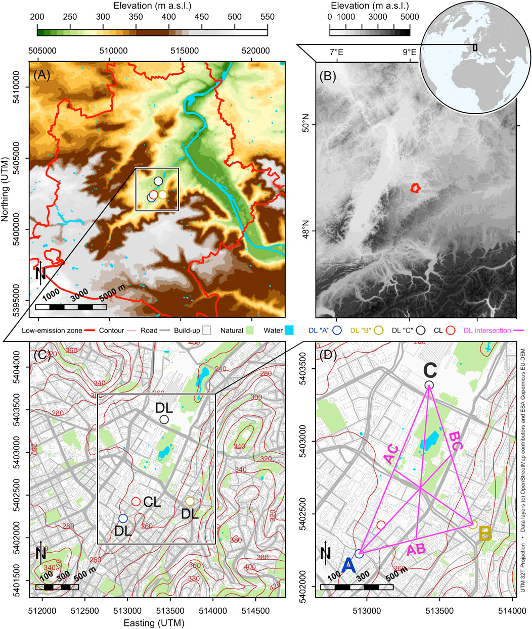
FIGURE 1. Situation of Stuttgart, Germany, showing (A) the local topography, (B) the complex regional topography, and (C,D) the locations of Doppler lidar (DL) and ceilometer (CL) systems in the City Centre. Except for (B), the coordinates are shown in UTM projection.

The investigation of the urban atmospheric boundary-layer structure and its temporal evolution requires frequent observations with sufficient spatial coverage. A dense spatial network of observations can help reveal patterns in the structure of the atmospheric boundary layer and the interactions between the surface and the atmosphere. However, the deployment of tall tower structures and airborne sensors is restricted in the airspace above dense urban areas. Therefore, we must rely on other observational methods, including ground-based remote sensing. Doppler lidar (DL) and laser ceilometer (CL) use established optical methods for range-resolved remote sensing of wind field and atmospheric structure, respectively, from the ground up (Weitkamp, 2005). Wind speed information is determined by observing the Doppler shift of laser light scattered back by aerosols in the line of sight of the DL optics. With sufficient resolution in the temporal and spatial domain, DL systems complement traditional radio-sounding and tower-based wind profile observations (Chanin et al., 1989; Post and Cupp, 1990; Grund et al., 2001; Pearson et al., 2009; Wulfmeyer et al., 2015, 2018). Additional detail can be derived at the intercept of multiple DL beams, including the direct observation of wind vectors using two or more DL units (Mann et al., 2008; Choukulkar et al., 2012; Lane et al., 2013; Fuertes et al., 2014; Banta et al., 2015; Stawiarski et al., 2015; Pauscher et al., 2016; Choukulkar et al., 2017; Vasiljević et al., 2017). Cloud base height can be interpreted from gradients in the backscatter-intensity profile recorded by CL, from which the depth of the mixed ABL can be determined (mixing layer height, MLH; Emeis et al., 2004; Münkel, 2007). Current commercially available DL and CL instruments are sufficiently portable and rugged to be deployed on roof tops. Furthermore, ground-based optical sensors benefit from the use of tall buildings or topography, in order to achieve a sufficiently unobstructed view in densely build-up areas.

The aim of this study was to determine the temporal evolution of the vertical structure of the ABL in the City Centre of Stuttgart during weak-wind conditions, contrasting weak-wind episodes in winter and summer. Of particular interest were:

• The vertical structure of the ABL above the roof level, including layers below the MLH with a relevant role in pollutant transport;

• Identification of valley-scale circulations in relationship to topography, seasonality and synoptic flow;

• Wind field modulation related to heterogeneity in land-use and urban canopy roughness (build-up vs. open parks)

2 Materials and Methods

We combined the observations of DL and CL for the investigation of wind field and structure of the ABL above roof level. The three aims of this study required different modes of operation of the remote sensing systems. Each DL system can be operated independently to observe vertical profiles of wind direction, wind speed and vertical wind speed variance. This approach is robust and is well-suited for long-term observation. However, the DL systems can also be deployed to form a dynamic mesoscale network. Observations can be combined after alignment of the DL beams in two or three spatial dimensions and time. The advantage of such a concerted multi-DL operation is that the computation of wind vectors can be simplified. The wind vectors are determined directly, are more local and can be observed at any location within the unobstructed range of the DL systems. Moreover, this mode of operation allows for observations of the wind field much closer to the roof level. However the concerted modes depend on the successful operation of a network of systems, which may fail if any of the individual systems is not functioning optimally.

The observations were part of a complex empirical campaign that involved other research groups and interests. The overarching campaign focus in 2017 involved experimental observation of representative periods of a few days for which weak-wind and limited cloud cover conditions were forecast by the local branch of the national weather service (DWD Stuttgart observatory “Schnarrenberg”; approximately 6 km north of Stuttgart City Centre). Those conditions were expected to severely impact air quality. A concerted DL approach was given priority during two intense observation periods (February 2017, July 2017), in order to acquire comparable results in both seasons and to accommodate shared interests with other research teams participating in the experimental campaign. The campaign and DL modes are detailed below.

2.1 Field Experiment

The experiment took place as part of a Federal Ministry of Education and Research (BMBF) initiative on Urban Climate Under Change [UC]², in which three-dimensional observations of atmospheric processes in cities (Module B, 3DO) were collected to support the development of a new national numeric fluid-dynamics model (Module A, MOSAIK) and decision-making models (Module C) for assessment of air quality and climate aspects in urban planning (Maronga et al., 2019; Scherer et al., 2019a; Scherer et al., 2019b).

Three “3D” scanning Doppler lidar units (model StreamLine XR, Halo Photonics Ltd., Worcester, United Kingdom) were deployed in a triangular configuration in the inner city of Stuttgart between 08 February 2017 and 08 August 2017 (Figure 1). DL observe Doppler shifts in the backscatter of (pulsed) laser beams, from which wind velocity is estimated using a Gaussian-filter aggregation into range gated intervals along the line of sight (Pearson et al., 2009). The laser beam of each DL can be programmatically directed in an approximately half-hemispheric domain, hence “3D” for its three-dimensional scanning optical remote-sensing application. For the conditions at the study site we expected the DL units to be most effective below 2 km range. Therefore, the separation between the DL units was limited to be on the order of 1 km, at rooftop locations with a maximum field of view and an unobstructed sight between the DL units (Figures 1D, 2). The azimuth angles of the DL beams were coordinated and recorded in relation to the instrument attitude. The instrument attitude, i.e., the azimuth offset to north, was determined by targeting objects within range at coordinates known from geo-referenced aerial views. In addition, each DL was equipped with a global positioning system (GPS) receiver and mobile phone network internet access for timekeeping and remote system management, respectively. For most of the observation period the DL units were configured to output computations for 18 m range gates and 1 s time integration of 15 kHz laser pulses.

FIGURE 2

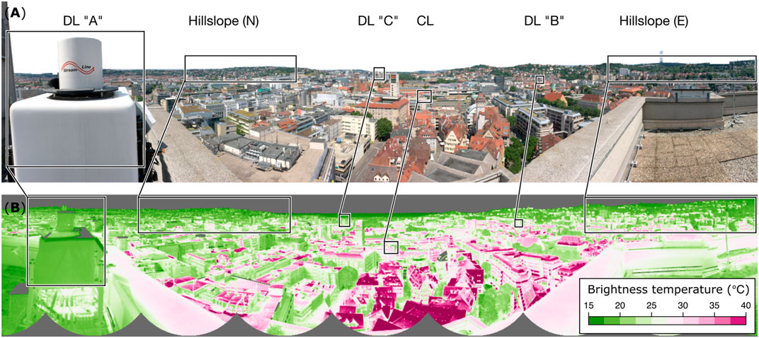
FIGURE 2. View from the roof-top location of Doppler lidar (DL) unit “A” towards DL “B” and DL “C,” the ceilometer (CL) and hillslopes in approximately Northern and Eastern direction, shown as (A) a digital camera still image and (B) a composite of thermal infrared images.

A laser ceilometer instrument (CL; model CL51, Vaisala, Helsinki, Finland) was deployed on a rooftop nearby and observed vertical profiles of backscatter intensity at 1 min time integration (Figure 1). Data were transferred from the DLs and CL periodically for off-site processing. Mosaic images of surface brightness temperature were composed from thermal infrared camera images (model PI-450, Optris GmbH, Berlin, Germany) and used here to evaluate spatial variability in surface thermal properties. Computations were performed using Python (Jones et al., 2001, SciPy scientific computing tools), Matlab and R (R Development Core Team, 2018).

2.2 Doppler Lidar Scan Routines and Schedules

Three DL systems were deployed on rooftops and are referred to here as DL “A,” “B,” and “C” (Figures 1D, 2, 3). The DL units were operated as a network with independent and concerted modes of operation (Table 1). The scan direction was set by waypoints, a combination of azimuth (α) and elevation angle (β), and the radial speed of the DL optics between waypoints.

FIGURE 3

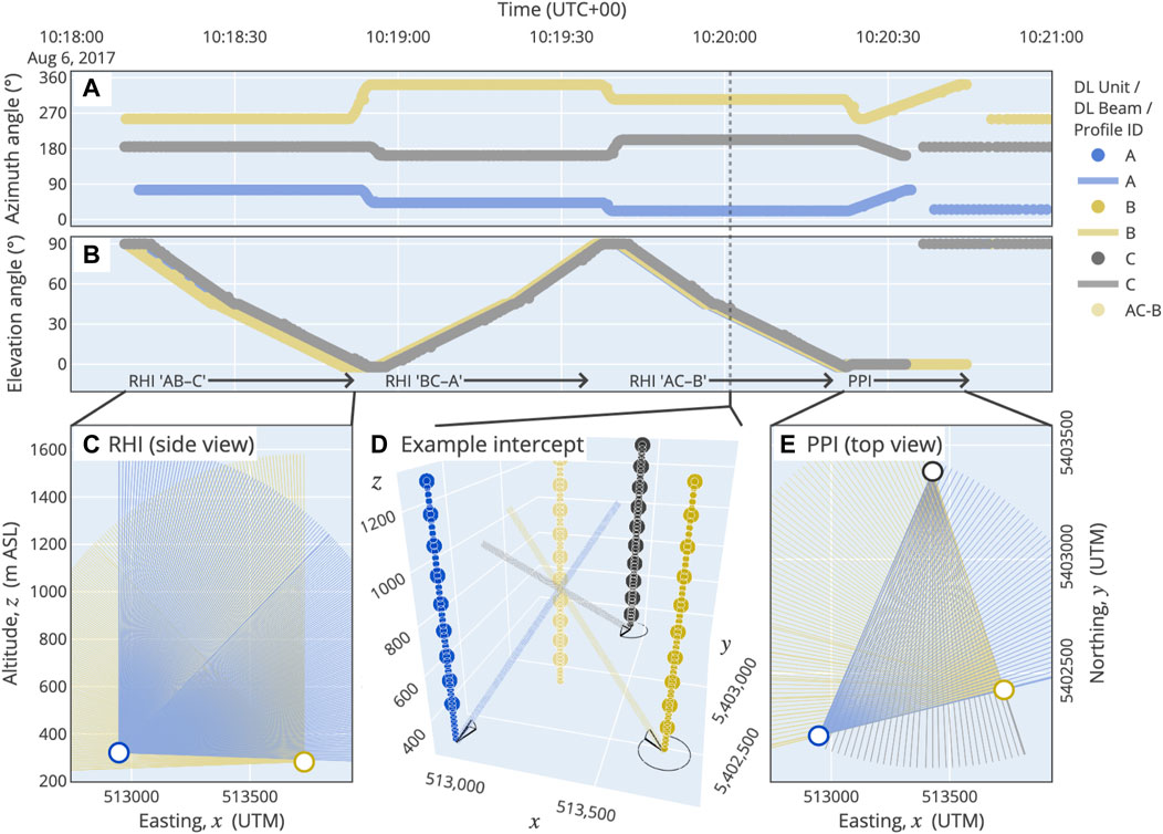
FIGURE 3. For an example Doppler lidar (DL) scan routine are shown the polar angles in (A) azimuth and (B) elevation, which includes (C) a range-height indicator (RHI) co-axial plane scan, (D) three-dimensional vertical profile intercepts and (E) a plan-position indicator (PPI) co-axial plane scan between DL units “A,” “B” and “C.” See text for details.

TABLE 1

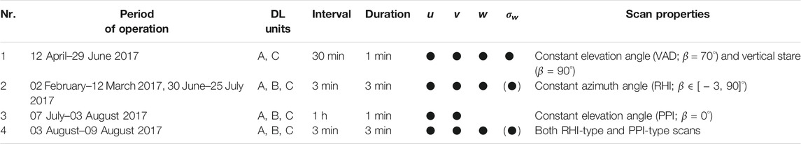
TABLE 1. Concerted Doppler lidar (DL) scan routines during the 2017 experimental campaign in Stuttgart City Centre.

The independent scan mode is the most common use of DL systems to determine vertical wind profiles above the location of the DL system. Between 14 March 2017 and 29 June 2017, DL unit “A” and “C” were configured to observe vertical wind profiles twice in the hour by applying a sine fit to so-called velocity-azimuth display retrievals (VAD; at 00′ and 30′ in the hour; α ∈ [0, 360)°; β = 70°; Table 1, Scan routine 1; see, e.g., Browning and Wexler, 1968; Weitkamp, 2005) and measured vertical wind speed otherwise. During this period, DL unit “B” was removed for unscheduled repair.

Scan routine 2 was the main concerted mode of operation of the DL network. Each DL system recorded a sequence of three elevation plane scans, with two scans in an azimuthal direction towards each-other and one scan in the azimuthal direction of the halfway point between the first pair of DL systems (Figure 3C; Table 1). The scan trajectories were pre-configured using waypoints starting at an elevation angle below the horizon (β = − 5^°) to the zenith position (β = 90°; idle mode) in three sections with a constant azimuth angle and an increasing angular velocity for elevation; a so-called range-height indicator scan (RHI; see Figures 3A,B, the periods with changing elevation angle with time; Figure 3C). Two DL systems were directed towards each-other to form a co-axial elevation plane (Figure 3C). A third DL system was directed to scan an elevation plane above a location halfway in-between the first two DL systems. These three scans overlap in a virtual vertical profile (Figure 3D). Hence, at the intersection of three DL beams in these scans, three components of the local wind vector were determined. The concerted scan is repeated to capture the virtual vertical profiles at half the distance between the remaining sections between the DL systems (Figure 1D; scan sections indicated by “AC,” “AB,” and “BC”).

Scan routine 3 involves a concerted horizontal plane scan at roof level and was scheduled once in the hour during the early summer period. These are so-called co-axial plan position indicator scans (PPI; β = 0°; Figure 3E; Table 1).

Scan routines 2 and 3 were combined into a single sequence in scan routine 4. Slight modifications were made to improve the timing of the observations, increase the number of useful observations in each scan section and add a horizontal plane scan within the same 180 s interval as scan routine 2 (Figure 3). The combination reduced the time penalty caused by measurement initialization, i.e., the DL mirror movement towards the first and from the last scan waypoint. This in turn allowed more detailed observation of the co-axial elevation planes. The azimuthal plane scan was made at the end of the sequence in scan routine 4 (PPI; β = 0°; Figure 3E, between approximately 145 and 180 s) of the unobstructed azimuthal sector of view between the three DL units (Figures 1D, 2, 3E).

As describe above, scan routines 2 and 4 involved a sequence of three simultaneous elevation plane scans within 180 s, in-between different DL pairs (RHI-type scans between units “A” and “C,” “A” and “B” and “B” and “C”; Figures 1D, 3; Table 1). By combining all DL observations within the 180 s interval we could compute an additional four vertical wind profiles at the emerging intercepts, i.e., above each DL system and in the center of the DL network (Figure 1D). At these additional intersections, the timing between three DL beams may be off by up to 120 s. Hence we must assume stationarity within the 180 s intervals to allow this method. As this is unlikely for small-scale perturbations in convective conditions, we consider only larger scale ($>100$ m) patterns for such results.

Please note that these additional four vertical profiles are only included in spatial presentations of the wind field (i.e., top-viewed maps of the wind field). Please also note, that in the presentation of vertical profiles against time we combine results in a composite sequence for the three main locations (Figure 1D; those vertical profiles midway between the DL systems, i.e., midway along sections “AC,” “AB,” and “BC”). These wind profiles are shown in sequence, the results are not averaged spatially.

In addition to the vertical wind profiles at the intersection of three DL beams, we computed covariant wind vectors u_α, v_α and w_α at the intersections of two DL beams. This was done for locations where two elevation plane scans aligned along the same azimuthal axis (Figure 1D, sections “AC,” “AB,” and “BC”).

2.3 Data Processing

2.3.1 Doppler Lidar Wind Vector Computation

The representation of results in a Cartesian coordinate system (x, y, z) required conversions to and from polar coordinates (azimuth, elevation, origin, distance) relative to the recorded DL attitude. First, the scan routine waypoints were computed prior to the measurements for each of the three DL systems, to allow a concerted observation along vertical profiles (Figures 1D, 3D). Second, post-measurement computations were required to derive wind vectors from the radial velocity observations at the intercepts of the DL beams. Both two- and three-dimensional wind vector components were computed for volumes in range of the DL systems, represented by a regular array of partly overlapping spheres (Stawiarski et al., 2013; Fuertes et al., 2014). Here, such an array with spatial resolution d is represented by spheres with a $[d\cdot \sqrt{3}]$ diameter. Grid arrays of 20 and 100 m were computed up to a vertical depth of 3,000 m.

The wind vector velocity components at the DL beam intercepts were derived as, Eq. 1,

$\left[\begin{array}{c}\hfill u\hfill \\ \hfill v\hfill \\ \hfill w\hfill \end{array}\right]={\left[\begin{array}{ccc}\hfill \cos ({\beta }_{\text{A}})\cdot \sin ({\alpha }_{\text{A}})\hfill & \hfill \cos ({\beta }_{\text{A}})\cdot \cos ({\alpha }_{\text{A}})\hfill & \hfill \sin ({\beta }_{\text{A}})\hfill \\ \hfill \cos ({\beta }_{\text{B}})\cdot \sin ({\alpha }_{\text{B}})\hfill & \hfill \cos ({\beta }_{\text{B}})\cdot \cos ({\alpha }_{\text{B}})\hfill & \hfill \sin ({\beta }_{\text{B}})\hfill \\ \hfill \cos ({\beta }_{\text{C}})\cdot \sin ({\alpha }_{\text{C}})\hfill & \hfill \cos ({\beta }_{\text{C}})\cdot \cos ({\alpha }_{\text{C}})\hfill & \hfill \sin ({\beta }_{\text{C}})\hfill \end{array}\right]}^{-1}•\left[\begin{array}{c}\hfill v_{\text{rA}}\hfill \\ \hfill v_{\text{rB}}\hfill \\ \hfill v_{\text{rC}}\hfill \end{array}\right](1)$

in which u, v and w are vector components along the three Cartesian dimensions x, y and z, respectively. The radial velocity, v_r, denotes the wind speed along a DL beam in unit m s⁻¹. The elevation angle β ∈ [−10, 90]° and azimuth angle α ∈ [0, 360]° are defined such that zenith (the vertical point overhead) is where β = 90°, and azimuth is observed clockwise with α = 0° pointing north and α = 270° pointing west. The subscripts A, B, and C denote the three DL units (Figure 1). DL observations with a signal-to-noise ratio (SNR) of less than −15 dB were excluded. If the centers of more than one range gate along a beam were aligned with the same grid cell volume, the radial velocity was averaged before computing vector components. Wind direction (φ) and wind speed (U_H) were computed for each grid cell and time interval as $[270°-\mathrm{a}\mathrm{r}\mathrm{c}\mathrm{t}\mathrm{a}\mathrm{n}\mathrm{2}$ $(\bar{u},\bar{v})\cdot 180\cdot {\pi }^{-1}]$ and $[\sqrt{{\bar{u}}^2+{\bar{v}}^2}]$, respectively. The outcomes of Eq. 1 can become sensitive to variability in v_r when the DL beams are closely aligned in one or more polar axis. Therefore, observations with an angular difference of less than 30° were excluded.

2.3.2 Ceilometer Cloud Base and Mixing Layer Height Computations

The cloud base height (CBH) up to 9,000 m above ground level was determined from the CL backscatter records and computed by the instrument software. The mixing layer height (MLH) was determined from CL observations using a development version of the BL-View software application (Vaisala GmbH, Helsinki, Finland). The MLH computations are based on the detection of gradients in CL backscatter signal (Emeis et al., 2004; Münkel, 2007). The computations use radio sounding data from the nearest weather station for reference and validation (DWD station Schnarrenberg is located approximately 6 km north of the Stuttgart City centre). From the CBH time series we computed the number of cloudy periods, as a proxy for cloud cover and development. For the computation we define day time as the period between 06:00 UTC to 18:00 UTC for the whole year instead of using a weighing function to compensate for day length differences between winter and summer.

2.4 Validation and Model Comparison

The backscatter signals from DL and CL were compared for validation purposes (See Supplementary Section S1.1). For validation of the wind profile results, high-resolution radio sounding data from the DWD Schnarrenberg station were used (See Supplementry Section S1.2).

A comparison was made between the empirical outcomes and a recently completed model simulation that matches the area in this study (see, e.g., Bahlouli et al., 2020; Zum Berge et al., 2021) and follows the approach by Talbot et al. (2012). A summary of the model configuration has been included in the supplementary material (see Supplementary Section S1.3). Here, the comparison serves as an exploratory exercise to assess the differences between the presented high-resolution empirical approach and typical, state-of-the-art model outcomes.

3 Results

3.1 Vertical Structure of the Atmospheric Boundary Layer

3.1.1 Cloud Base and Mixing Layer Height

From the CL data we can derive information about the depth and upper boundary of the ABL. First, the cloud base height in winter (January to February 2017 and November to December 2017) revealed frequent presence of low clouds (fog) that persisted throughout the day (Figure 4B; see also Supplementary Figure S5). Second, the lowest detected cloud layer in late spring through summer and early fall (May to September 2017) showed a consistent increase in height from morning hours to late afternoon (Figure 4B). The CBH typically increased upward of 1,000 m depth around noon, on some summer days between 2,000 and 3,000 m depth in the afternoon. Third, cloud cover was less continuous in summer months and showed intermittency during day time (Figures 4B,C). The intermittent presence of clouds often coincided with the occurrence of hydrometeorological events (see also Supplementary Section 1.2, precipitation identified by enhanced CL backscatter). The short-lived cloud cover and precipitation can be interpreted as convective cells advecting through the observed area. Fourth, CBH and MLH increases correlated to seasonal differences in day length. The daytime changes were typically detectable from approximately one to 2 hours after sunrise (Figures 4A,B; see also Supplementary Figure S5). Fifth, the MLH showed similar patterns as the CBH, when comparing summer and winter months. Although the MLH and the lowest detected CBH showed good agreement, additional layers were occasionally identified below the lowest cloud base height (Figures 4A, 5; Supplementary Figure S5). Sixth, the MLH could not be determined as a continuous time series as is made clear from the many gaps, particularly during the day (Figure 5).

FIGURE 4

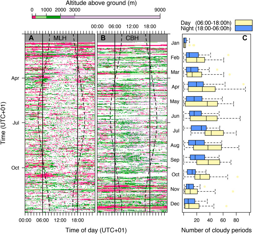
FIGURE 4. The (A) mixing layer height (MLH), (B) the cloud base height (CBH) and (C) a the number of cloudy periods during the day and night per month are shown for Stuttgart City Centre. Day time was defined as the period between 06:00 UTC to 18:00 UTC and sunset and sunrise times are shown in the left panels as dashed lines.

FIGURE 5

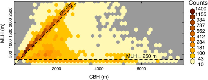
FIGURE 5. Correlation between cloud base height (CBH) and mixing layer height (MLH) above Stuttgart City Center during 2017. Dashed lines highlight the identity and MLH of 250 m. See text for details.

When structure of the ABL is concerned in relationship with air quality, the development of layers below the CBH is of particular interest. The CL backscatter signal is correlated with the density and particle composition of aerosols. It is important to note that the lowest identified level of MLH and the CBH did not always coincide (Figures 4, 5; Supplementary Section S1.1). A frequently reoccurring MLH depth was identified at approximately 500 and 250 m depth, also when the lowest cloud base was substantially higher. Furthermore, occurrences with a MLH (or CBH) at the lower reoccurring depth were not equally distributed throughout the year, and occur predominantly at night and in winter months (Figure 4).

A comparison of the time of occurrence of clouds with vertical motion is not included in this study. We experienced that this requires a more thorough investigation into the separation of cloud and precipitation events (See Supplementary Section 1.2).

3.1.2 Vertical Wind Profiles

Seasonal and diurnal patterns in the wind profile were derived from the Doppler lidar results and confirmed by nearby radio sounding data.

The wind direction above 750 m above sea level (a.s.l.), or approximately 500 m ABL depth, was dominantly west between March 2017 and June 2017 (Figure 6; see also Supplementary Section S1.1). The prominence of the western wind sector between 750 and 1,150 m a.s.l. altitude was evident for much of the day. Below 750 m a.s.l. (500 m depth) the wind profile statistics derived from both DL and RS showed more variable wind direction as well as differences between day and night (Figure 6; Supplementary Figure S2). Below that altitude range wind direction was revealed to shift to southwest at night and to northeast during the day, particularly after noon (Figure 6A).

FIGURE 6

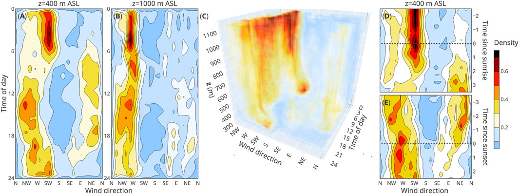
FIGURE 6. Frequency of occurrence of wind direction against time of day and altitude above sea level (z; m ASL) for the period 14 March 2017 to 29 June 2017. (A,B) show cross-sections at 400 and 1,000 m, whereas panels (D,E) show cross-sections at 400 m with time as hours since sunrise and sunset, respectively. See text for details.

Wind direction changes occurred around sunrise and sundown. At this latitude, the sunrise and sundown times transition several hours over the course of the season (see, e.g., Figure 4B), hence it is meaningful to take sunrise and sundown as reference for analysis over a longer periods. The alignment of the wind vector data with sunrise and sunset set as time reference revealed a pronounced wind direction shift during the diurnal morning and evening transitions (Figures 6D,E).

At 400 m a.s.l (150 m depth), nighttime wind direction was dominantly southwest until 1.5 h after sunrise, thereafter the wind direction shifted to a northeast to northwest sector (Figure 6D). At sundown, a west to northwest wind direction sector was prominent, transitioning to a northwest to southwest sector approximately 1.5 h after sundown (Figure 6E). A southwestern wind sector was least likely in the hours before sunrise and during the day, but does occur during the transition after sundown (Figure 6E). Please note that these wind direction patterns included all synoptic conditions, and are not limited to the weak wind case. The vertical extent of the layer with a deviation in wind direction near roof level is approximately 500 m a.s.l. (250 m depth), which is consistent with the CL results for mixing layers described above (Figure 4C).

If we take a close look at the topography immediately surrounding Stuttgart City Center, we can infer that channeling of the roof-level flow into a southwest to northeast axis could be expected (Figure 1A). However, the exact wind profile properties cannot be inferred from a map. We continue with a closer look at spatially distributed wind profiles during typical weak-wind episodes in winter and summer.

3.2 Valley-Scale Circulations

3.2.1 Spatially Distributed Vertical Wind Profile Observations

The concerted Doppler lidar mode produced time series observation for three (and up to seven) spatially distributed vertical wind profiles. The results reveal detailed patterns above roof level for selected weak-wind days in winter and summer. Please note that we first discuss the temporal patterns in the wind profiles (Figures 7A,B, 8A,B).

FIGURE 7

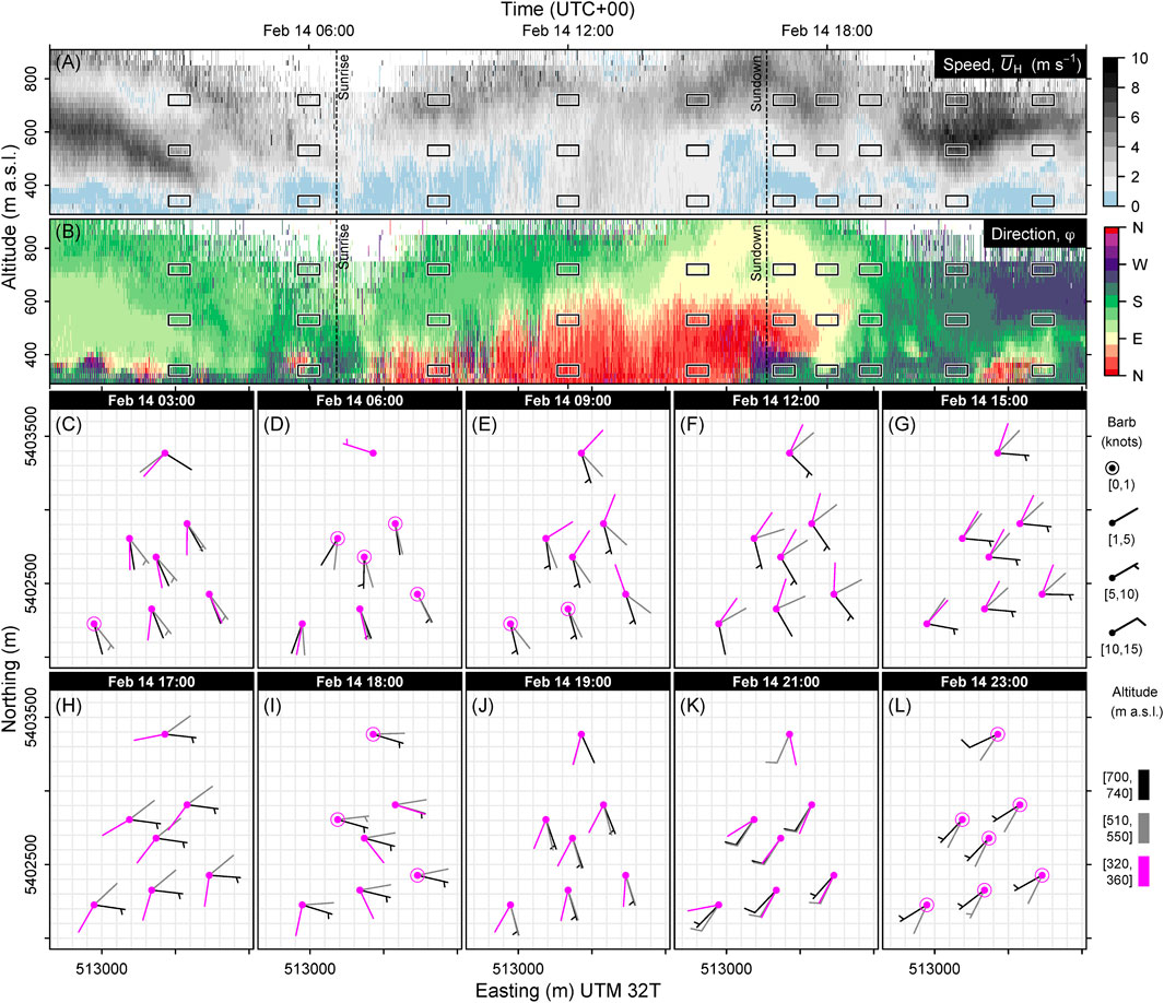
FIGURE 7. For a selected weak-wind day in winter (14 February 2017), a composite of the vertical profiles in Stuttgart City Centre of (A) the wind direction and (B) the wind speed are shown together with (C–L) the mean wind field for selected locations, altitudes and periods in an area corresponding to Figure 1D. The altitudes and periods are annotated in panels (A,B) by black rectangles.

FIGURE 8

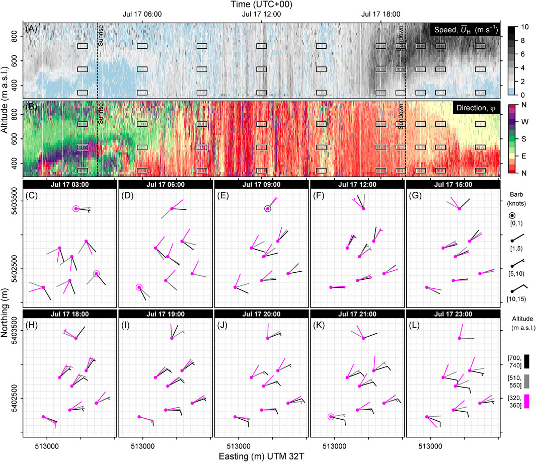
FIGURE 8. For a selected weak-wind day in summer (17 July 2017), a composite of the vertical profiles in Stuttgart City Centre of (A) the wind direction and (B) the wind speed are shown together with (C–L) the mean wind field for selected locations, altitudes and periods in an area corresponding to Figure 1D. The altitudes and periods are annotated in panels (A,B) by black rectangles.

For the winter case, consistent modes of flow modulation were revealed (Figures 7A,B), which we separate in a daytime and nighttime phase. Below approximately 600 m a.s.l. (350 m depth), a level that is similar in height to the surrounding topography, the wind speed is low and wind direction intermittent. Starting after sunrise, a weak-wind layer up to 600 m a.s.l. (350 m depth) developed immediately above roof level with a north to northeast wind direction, below a layer aloft with a dominant south to east wind direction and a higher magnitude wind speed. The situation changes at sundown (16:30 UTC), after which a weak south to southwest flow undercuts the north to northeast flow that developed during the day (Figures 7A,B). We can interpret the latter as shallow drainage flow from the surrounding hills, decoupled from the regional flow. Above approximately 400 m a.s.l. (150 m depth), the wind speed increases after sundown and reaches a maximum between 450 and 600 m a.s.l. (200 and 350 m depth).

In the summer case, longer days and higher solar influx lead to a more eventful daytime evolution of the ABL, also during day of predominantly weak-wind conditions (Figures 8A,B). First, an abrupt transition was found near roof level in the early morning. Similar to the selected winter day, a pattern developed in the early hours after sunrise with inflow into the City Centre from a north to northeast direction (Figure 8B). Second, the wind speed and wind direction profile develop much more intermittently during the representative summer day.

Weak wind days are often part of episodes of stable synoptic conditions. Hence, we can compare the results for the selected days with other days during those weak wind episodes. We compare the days of winter for the period between 13 and 16 February 2017. A repeating pattern of the diurnal evolution of the wind profile could be recognized on these calm winter days (Figure 9). The ABL reached up to approximately 750 m a.s.l (or 500 m depth) during the day and showed super-positioning of layers with significant differences in wind speed and wind direction as described for 14 February 2017 above (Figures 7, 9). The weak-wind winter episode ends when a storm front arrived on the evening of 16 February 2017 as highlighted by cloud cover and precipitation (Figure 9E). However, a similar diurnal pattern developed again after passing of the storm on the 18 February 2017 (not shown). On each weak wind day during this episode, a weak flow from a north to northeast direction developed at roof level from around sunrise. This layer generally increases in depth until the afternoon, and appears to develop independently of the wind direction in the layers aloft (Figure 9). Around sundown the situation changed abruptly, when flow from the southwest initially undercuts (e.g., 14 February 2017) or replaces (e.g., 15 February 2017) the layer that developed during the day (Figure 9). After sundown, the wind field near roof level showed a dominant flow from southwest to southeast direction, with intermittent excursions to other directions throughout the night (Figure 7B), including periodical alignment with the flow aloft (e.g., Figures 3, 7 03:00 and 21:00). Nevertheless, the layer that established near roof-level during the night, as recognized by a low wind speed and directional shear, did not appear to exceed 500 m a.s.l. (250 m depth). Above this shallow nocturnal layer, between roughly 500 and 700 m a.s.l. (250 and 500 m depth), the wind speed increased to a maximum, periodically exceeding 5 m s⁻¹, then decreased further aloft (Figure 9).

FIGURE 9

FIGURE 9. Vertical profiles of (A) wind direction (φ), (B) horizontal wind speed $({\bar{U}}_{\text{H}})$, (C) vertical wind speed $(\bar{w})$, (D) Doppler lidar backscatter (DLB) signal and (E) the ceilometer backscatter (CLB) signal are shown for Stuttgart City Centre during the period 13 February 2017 to 16 February 2017. The ceilometer-derived cloud base height and mixing layer height are shown in (E) as white triangles and magenta diamonds, respectively.

Representative summer episodes of weak-wind conditions confirmed similar patterns as found for the selected summer day discussed above. First, the ABL in summer developed significantly deeper under convective forcing, as shown by both DL and CL data (see Supplementary Figures S10, S11). Second, The vertical profile on weak-wind summer days showed a north to northeast wind direction near roof level after sunrise, also similar to winter, and also shifting to a north to northwest wind direction sector later in the morning (see Supplementary Figure S10; e.g., 04 July 2017, 05 July 2017 and 06 July 2017; 17 July 2017 and 18 July 2017). Last, after sunrise, the variability in wind direction, wind speed and magnitude of the vertical wind speed increased rapidly. This is in line with the CL findings that indicated a rapidly rising CBH and MLH.

3.2.2 Horizontal Wind Field

In the following section we focus on the spatial patterns within the observed volume between the Doppler lidar units, again by investigating the relationship between the flow near roof level and further aloft. Based on the results discussed above we distinguish three altitude levels that represent a level near the roof, a level near the top of a (assumed) topography-channeled layer and a level further aloft that is assumed to represent synoptic flow, at 340, 530 and 720 m a.s.l., respectively.

The seven vertical profiles observed by the concerted modes should be expected to show a high level of correlation by their proximity within a 1 km radius. It allows us to compare both vertical and horizontal alignment of the wind profiles within the observed domain.

Separating the individual vertical profiles showed spatial deviations in the wind field, both horizontally and vertically (Figures 7, 8; Supplementary Figures S6–S9, particularly panels C to L therein). Generally, patterns of convergence/divergence were revealed when comparing the wind vectors at similar altitudes, as well as patterns of directional shear between altitude ranges. However, presenting the wind profile data spatially revealed those patterns more clearly. On all weak-wind winter days, substantial directional shear ($>60$°) within the vertical profile is again confirmed, particularly below 500 m a.s.l. (below 250 m depth; Figures 7E–G). Interestingly, for a period with flow from north we see indication of divergence, which was most evident near roof level in the south of the observed domain (Figures 7E–G), whereas for a period of west to southwest flow at the same profile locations convergence can be found (Figures 7H–K). This again confirms a process of channeling of the flow by the surrounding topography, locally modulating the wind field in the lowest 150 m in the City Centre.

For the summer period we compared the wind field patterns on three selected days, each with a different dominant day-time synoptic wind direction above 720 m a.s.l., representing northwest, northeast and east-southeast synoptic wind directions on 04 to 05 July 2017, 17 July 2017 and 18 July 2017, respectively. On all 3 days, wind magnitude increased throughout the vertical profile after the morning transition and wind direction aligned below 720 m a.s.l (500 m depth) between 9:00 and 12:00 (Figures 8F–H; see also Supplementary Figures S6–S8). During summer, evidence of directional shear in the vertical profiles is evident after sunset, coinciding with low wind speed at the lowest altitude levels. A particular pattern of wind direction changes between the seven profiles was indicative of a rotation (converging or deflected flow; Figures 8J–L). For instance, on 17 July 2018, the general daytime flow direction is north to northeast, however, the lowest profile height profile the location furthest north showed a consistent north to northwest direction (Figure 8). We interpret this as a clockwise rotating motion near roof-level within the topographic boundaries of Stuttgart City Centre.

The spatial correlation and alignment in wind direction was tightly related to wind speed and time of day. For example, on 18 July 2017 the wind speed up to 1,000 m a.s.l. (750 m depth) increases until after sundown with a direction from east-southeast (Supplementary Figure S8). Thereafter, the vertical and horizontal alignment appeared to collapsed between 20:00 and 21:00, as wind speed dropped below 5 m s⁻¹ near 530 m a.s.l, or 280 m depth.

A model simulation for the representative winter day (14 February 2017) confirmed the predominantly south synoptic wind direction in the area, including a shift to a southwest direction at the end of the day (Figure 10). The model results also showed that topography in such weak wind scenarios induced a channeling effect on the flow in the lower 500 m of the ABL (Figure 10).

FIGURE 10

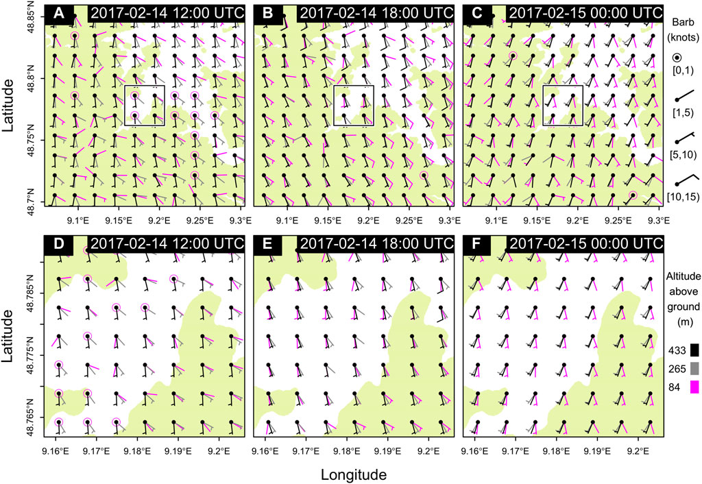
FIGURE 10. The spatial mean modelled velocity fields at three model altitude levels and at 12:00, 18:00 on 14 February 2017 and 00:00 on 15 February 2017 are show for the Stuttgart area (top) and Stuttgart City Centre (bottom), corresponding to the areas shown in Figures 1A,C, respectively. Topography with an elevation exceeding 300 m a.s.l. is highlighted in the background in light green.

3.3 Impact of Surface Heterogeneity

We evaluate below to which extent the observed concerted Doppler lidar wind profiles, horizontal and vertical, can be correlated to differences in surface characteristics.

Please recall that a horizontal wind component (covariant, azimuthal) and vertical wind statistics were determined from elevation plane scans between pairs of DL systems (scans with constant azimuth and variable elevation angle; Figure 1D, along sections “AB,” “BC” and “AC”; Table 1). For evening-transition of the selected weak-wind winter case, a multitude of apparent internal boundary layers can be found in-between the locations of the vertical profiles (Supplementary Figure S15). The horizontal wind speed profiles were consistent with spatial distance, but varied with altitude. Please note that wind magnitude along an elevation plane only equals the horizontal wind speed if the wind direction is aligned with the plane. The co-variant wind speed showed a maximum in the elevation plane between DL system “A” and “B” (along section AB), at approximately 800 m a.s.l. (550 m depth) at 17:00 on 14 February 2017 (Supplementary Figure S15A; Figure 7H). During this period there was no significant lateral difference or variability in vertical wind, despite the significant directional shear in the vertical profile between height levels (Supplementary Figures S15E–G). Furthermore, the apparent nocturnal alignment of the vertical profiles between the DL systems showed no indication that the heterogeneous surface properties, in the area itself or upstream, had an impact on the vertical motion. This confirmed the (directly) observed vertical wind speed profiles for the same period.

The daytime situation on the selected winter day again showed a different dynamics. The results showed spatial and temporal differences in vertical motion within the observed area (Figure 11). Short periods of updraft are assumed to be correlated to weak thermals. Such periods of updraft were most prominent in the southeast of our observation domain (DL unit “A”) and least significant in the north (DL unit “C”) (Figure 11). Vertical motion in excess of 1 m s⁻¹ was recorded above DL unit “C” in the lowest part of the vertical profile (Figure 11F). This was also confirmed at the same locations by the co-variant elevation plane results (Figure 5; Supplementary Figure S15).

FIGURE 11

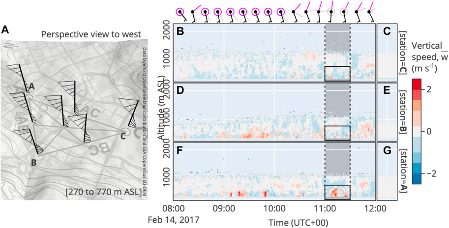
FIGURE 11. Shown for locations in Stuttgart City Centre are (A) the mean wind profiles for the highlighted period and altitude range in the right panels in a perspective view with a topography background, and (B,D,F) the vertical wind speed against time and altitude above DL station locations “A”, “B” and “C”, and (C,E,G) the mean vertical wind speed against altitude for the period between 08:00 and 12:00 UTC on 14 February 2017. Wind barbs shown on top represent the 15-min mean direction at 340 m, 530 and 720 m a.s.l., in magenta, grey and black, respectively.

In summer, thermally driven vertical motion developed during the day that was shown to be persistent above the three DL stations for minutes at the time. This was independent of the predominant wind direction (see Supplementary Figures S12–S14). Phases of updraft and, subsequently, downdraft, were present at the three DL station locations, but we could not derive a clear link from the timing and magnitude of such cells. None of the DL locations showed a bias in the mean vertical motion that would help identify the proximity of a spatially persistent thermal hot-spot.

We analyzed relationship between horizontal and vertical wind field on 06 August 2017, which was similar in wind conditions to 17 July 2017 (see Supplementary Figures S7, S9). Please recall that the horizontal wind field was determined at approximately roof-level from co-planar azimuthal scans operated in late summer (Figures 3, 12; Table 1; Supplementary Figure S9). The development of a 10 min long period of updraft near the location of DL unit “A” coincided with lower wind speed and convergent wind direction towards a nearby local horizontal wind speed minimum (Figures 12A,B). Please note that the horizontal wind speed also decreased towards location “B”, but this can also be explained by a gradient in measurement height above the roof-level (Figure 1), as DL unit “A” and “C” were deployed on tall-tower roof tops, approximately 20 m above the regular roof height on which DL unit “B” was deployed.

FIGURE 12

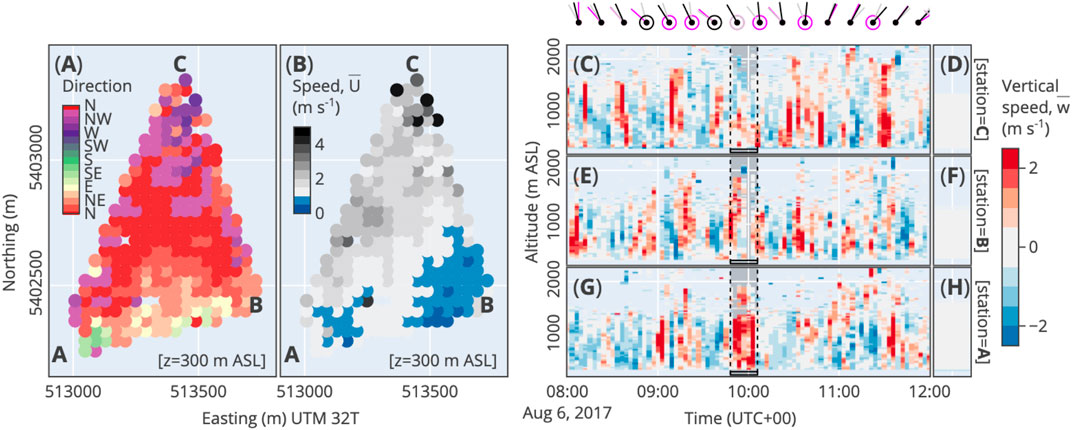
FIGURE 12. Shown for locations in Stuttgart City Centre are a top view of the (A) mean wind direction and (B) mean wind speed for the highlighted periods in the right panels, and (C,E,G) the vertical wind speed against time and altitude above DL station locations “A”, “B” and “C”, and (D)(F)(H) the mean vertical wind speed between 08:00 and 12:00 UTC on 06 August 2017. Wind barbs shown on top represent the 15-min mean direction at 340 m, 530 and 720 m a.s.l., in magenta, grey and black, respectively.

4 Discussion

4.1 Vertical Structure of the Atmospheric Boundary Layer

Conceptually, drainage flow is expected to occur from the surrounding hills (Hamm, 1969). The local topography provides boundaries from which we can formulate likely flow regimes. Conceptually, we can expect channelling effects along the major axes of the surrounding topography. The City Center is built in a debouching (widening) section of the Nesenbach valley. The Nesenbach eroded an inlet to the southwest of the City Centre and flows into the larger Neckar river to the northwest (Figures 1, 13). The surrounding ridges and plateau extent between 150 and 250 m above the City Centre valley bottom.

FIGURE 13

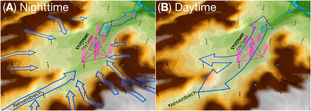
FIGURE 13. Conceptual diagram of competing flow regimes during weak wind conditions in Stuttgart City Centre for (A) night-time drainage flow and (B) topographically channelled flow during daytime. The perspective is viewed from the south. Black lines and points highlight the altitude up to 500 m a.s.l. in 100 m intervals, and vertical wind profiles are included for illustration purposes as magenta windbarbs. The topography and color gradient from Figure 1A are shown as background.

We interpret the nocturnal case as drainage flow competing with synoptic flow. The upper boundary of the drainage flow is forced by the surrounding topographic ridge and plateau (Figure 13A). The major drainage direction at our study site is presented by the Nesenbach valley, roughly forming a southwest to northwest axis, with minor channel inlets from the nearby steeper slopes (Figure 13A). This includes the Fischbach located southwest of our observation domain (Figures 1, 13). The presence of a (mostly) noctural wind speed maximum that decreased in altitude and intensity during the night is typical for decaying low-level jets (LLJs) observed in the region (Damian et al., 2014).

Dominant during the daytime was channeling of the flow along a similar major axis. This axis is likely to be prescribed by the southwest to northwest orientation of the plateau ridge to the east of the valley and the opening to the northwest of the Stuttgart City Center (Figure 13B).

The relatively short duration of cloud cover in summer and variability in (vertical) wind speed confirms the presence of convective cells advecting through the observation area.

4.2 Valley-Scale Circulations

Situations were observed with a net downward motion over a period of minutes, which can be explained by the proximity of steep topographic gradients (e.g., Supplementary Figure S14E, flow down a steep slope) or widening of the valley (e.g., Supplementary Figure S13E; flow down a contributory stream valley).

The recording of multiple profiles would in principle allow the investigation of the motion and structure of advecting thermal cells within the domain, particularly when the wind field is recorded in up- and downstream locations. However, the updraft periods during the selected weak-wind summer days were on the order of 3–10 min. A meaningful analysis of their development would require a higher temporal and spatial resolution than provided by the concerted DL method used here. Evidence of a link between spatially distributed vertical profiles could be established using the high resolution information about the horizontal wind field at roof level.

4.3 Impact of Surface Heterogeneity

The City Centre area includes different land-use elements, itself again in contrast to the forested hills surrounding the valley (Figure 2). For instance, there is an open area with a pond in the north half of the DL observed domain and a city park with grass fields and tall trees northwest of the railway station where DL unit “C” was deployed (Figure 1D). A stream re-surfaces in this park and flows north after being channeled below-ground in the City Centre. The industrial surface properties of the railway tracks in the north and the build-up area of the City Centre, in contrast to the vegetation and open water of adjacent parks and slopes, may have an assumed impact on atmospheric transport due to their differences in surface energy fluxes and roughness. The impact of such an unstructured heterogeneity on atmospheric processes was difficult to observe, or to predict, but it can play a dominant role in atmospheric transport processes (Bou-Zeid et al., 2020). In addition, recent studies in the same area showed that there are significant spatial differences in air quality, which could be related to local differences in emission strength as well as atmospheric transport (Samad et al., 2020; Samad and Vogt, 2020). However, using the described methods this could not be demonstrated by the observations.

We could determine the presence of thermal plumes, but could not link those to particular landscape features. Thermal plumes would result in convergence near the roof surface in combination with updraft motion (see, e.g., Omidvar et al., 2020). An indication of the effects of thermal plumes on both the horizontal and vertical profile could be found on 06 August 2017, which was similar in wind conditions to 17 July 2017 (see Supplementary Figures S7, S9). As our examples showed, the thermals were difficult to trace in space and time. However, we also lack an automated approach to determine their evolution and to connect patterns found in the different wind field results across space and time.

4.4 Limitations of the Methods

Each DL scan routine involves trade-offs. The concerted DL scanning routines applied in this study provided limited information about turbulence statistics (Scan routines 2, 3 and 4), whereas routines for independently operated DL systems (Scan routine 1) provided reliable turbulence statistics, but lacks spatial detail and are hindered by poor signal quality in the first (lowest) range gates. As the latter corresponded to a distance of $<63$ m from the instrument, or an altitude of approximately 320 m a.s.l., this coincided with layers of interest identified by the CL adn concerted DL results. In contrast, the concerted DL scanning approaches are more useful for discovery of high-resolution spatial patterns and allow observations of wind vector components down to the roof level.

At the upper boundary of the ABL, the concerted DL method did not consistently show valid wind profile results up to the lowest CBH or MLH as identified from CL observations. Hence, the interpretation of the ABL wind field and motion near the CBH, particularly in summer, was made difficult by the limited effective range of the DL at roughly 1,150 m a.s.l., or approximately 1,400 m from the DL system furthest away from the DL beam intercept (Figure 1; Supplementary Figure S10). The inclusion of poor quality DL data (SNR of −17 to −15 dB) and the integration of more data points (upto a interval of 100 m) could not help extent the observed vertical profile range (Figure 9; Supplementary Figure S10). Increased range gate width settings, adjusted focus range, longer laser pulse integration times and a reduction of the distance between the DL units may have improved the observable profile height to the MLH during the summer periods. A reanalysis of the high-resolution DL retrieval data with a different set of weight functions would be an option, but those high-resolution retrieval data could not be stored during this experimental campaign.

The mean vertical wind speed profiles showed some deviations that could, for example, be explained by misalignment of the DL observations. A possibility that cannot be ignored in such complex topography is that the vertical profiles (recorded at zenith angle) were not observed fully perpendicular to the streamline flow and therefore correlate to wind direction shifts. If a larger spatial domain would be investigated with a co-planar DL approach further way from the surface, this effect could perhaps be minimized (Adler et al., 2020).

Both the summer and winter ABL structure would be better explained with additional information on air temperature and moisture content. There was a vertical temperature profiling system installed in the City Centre during the campaign, but data at sufficient resolution would not be available. Moreover, the German legal framework for the use of unmanned aerial vehicles changed during the campaign, leading us to not deploy an available airborne monitoring platform.

In the model simulation, zones of directional shearing developed within the City Centre valley profile, albeit less pronounced as in the observations and not as strict along a southwest to northeast axis (Figures 10D–F). We should emphasize here that the more tight vertical coupling within the City Centre valley can stem from a smoothing effect by low-resolution topography input data (150 m; derived from a 30 m grid spacing elevation model), in combination with the terrain-following approach of the WRF model. We should also caution again, that the model simulation results only serve an exploratory purpose in this study and limitations are known. The model configuration may provide usable simulation results for areas at higher elevation and strong wind, e.g., for wind energy forecasting on the plateau, but the spatial resolution may appear excessively coarse when the same model is applied to more sheltered areas during weak-wind cases (see Supplementary Section S1.3 for model details). As an outlook this shows that progress is needed, for instance by using such DL-derived profiles in the validation of simulations in complex terrain. Using DL as additional boundary condition to drive such a model set-up currently comes at prohibitive numerical cost.

5 Conclusion

The combination of CL and DL retrieval methods helped identify seasonal to hourly patterns in the dynamics between the complex topography and the ABL in the Stuttgart City Centre valley.

• Topographic modulation of the ABL in Stuttgart, particularly the wind field, could be confirmed;

• Modes of valley-scale circulation and ventilation could be identified in relationship to the local topography, the seasonality and the synoptic flow;

• Clear evidence of the impact of (sub)mesoscale heterogeneity in land-use and roughness on the structure of the ABL could not be found, but methodological limitations may have played a role.

Although the retrieval range was more limited than expected, particularly in summer, the deployment of concerted DL systems in line of sight and close proximity proved useful for discovery research in such a complex urban landscape. The a duplicity of stand-alone DL retrievals proved mostly redundant. The concerted retrieval methods used in this study were not convincingly sensitive enough for the quantification of sub-mesoscale interactions, such as thermal plumes.

The winter case study exemplified the potential use of covariant elevation plane data to complement vertical wind profiles, but with limitations. First, the usefulness of the information about covariant wind components was mostly limited to periods of full alignment of the mean flow with the azimuthal axis of elevation plane. Second, the computed vertical wind speed information proved useful to reveal, or confirm, larger and more persistent spatial patterns in the dynamics with the surface. Third, the relatively long time interval of the observations negatively impacted the relevance of the co-variant results. Consequently, the more reliable vertical motion observation is the direct retrieval of vertical wind speed at zenith angle, limited to the locations of the three DL units.

Our results confirm earlier observations and assumptions about competing flow regimes during weak wind episodes in Stuttgart. The urban atmospheric boundary layer showed re-occurring patterns during the winter episode that included the development of a layer below a depth of 250 m, roughly coinciding with the ridge height of the adjacent topography, and developing mostly independently of the flow aloft during weak wind conditions. This included a shallow nocturnal layer of weak flow along a southwest to northeast axis (Nesenbach valley); the development of weak north to northeast flow into the City Center during daytime; and the evolution of nocturnal low-level jets aloft. In daytime during summer, the wind field near roof-top level showed tight alignment with the flow aloft. An apparent valley-scale circulation (horizontal rotation) could develop in the afternoon. Validation of the exact extent of the rotation would require continuous observations in a larger area and volume. Continuous, high-resolution wind field observations revealed a dominant diurnal pattern of flow in an out of Stuttgart’s City Centre that was tightly coupled to sunrise and sundown.

All these findings should be of importance for air quality forecasting, model development and urban planning.

Data Availability Statement

The datasets presented in this study can be found in online repositories, including https://doi.org/10.5281/zenodo.4045802.

Author Contributions

MZ and SE designed the experiment. MZ collected and analysed the data. MZ, CH, MK, DL, CM, AP, and RR provided interpretation of the data. MZ drafted the article. MK and DL provided critical revision of the article.

Funding

This work was funded by the German Ministry of Education and Research (BMBF) through the Urban Climate under Change (UC)² program (contracts 01LP1602G and 01LP1602). The Doppler lidar analysis methods were developed with support of the German Research Foundation (DFG; grant ZE 1006/2-1).

Conflict of Interest

Author CM was employed by the company Vaisala GmbH.

The remaining authors declare that the research was conducted in the absence of any commercial or financial relationships that could be construed as a potential conflict of interest.

Publisher’s Note

All claims expressed in this article are solely those of the authors and do not necessarily represent those of their affiliated organizations, or those of the publisher, the editors and the reviewers. Any product that may be evaluated in this article, or claim that may be made by its manufacturer, is not guaranteed or endorsed by the publisher.

Acknowledgments

We thank Jasmin Hofgartner (City of Stuttgart Environmental Protection Agency), Ulrich Vogt, Abdul Samad (both University of Stuttgart), Norbert Kalthoff, Andreas Wieser (both KIT), Uwe Schickedanz, Thomas Schuster, Sabine Krüger, Sarah Jäger, Clemens Steiner and Klaus Riedl (German Meteorological Service, DWD/RWB Stuttgart) for advice and support during the field campaign. We thank Carsten Jahn (KIT) for assistance in the field. We thank Volker Meyer (Wexford Immobilliengesellschaft GmbH), Michael Exner (Deutsche Bahn AG), Erhard Haak and Lutz Wegner (both Landeshauptstadt Stuttgart) for key efforts in support of the experimental campaign. The authors thank all partners, institutions and persons, involved in the [UC]² research programme for their contribution. The authors thank the editor Gert-Jan Steeneveld and two reviewers for their peer review.

Supplementary Material

The Supplementary Material for this article can be found online at: https://www.frontiersin.org/articles/10.3389/feart.2022.840112/full#supplementary-material

References

Adler, B., Kalthoff, N., and Kiseleva, O. (2020). Detection of Structures in the Horizontal Wind Field over Complex Terrain Using Coplanar Doppler Lidar Scans. Meteorol. Z. 29, 467–481. doi:10.1127/metz/2020/1031

CrossRef Full Text | Google Scholar

Banta, R. M., Pichugina, Y. L., Brewer, W. A., Lundquist, J. K., Kelley, N. D., Sandberg, S. P., et al. (2015). 3D Volumetric Analysis of Wind Turbine Wake Properties in the Atmosphere Using High-Resolution Doppler Lidar. J. Atmos. Oceanic Technology 32, 904–914. doi:10.1175/JTECH-D-14-00078.1

CrossRef Full Text | Google Scholar

Barlow, J. F., Halios, C. H., Lane, S. E., and Wood, C. R. (2014). Observations of Urban Boundary Layer Structure during a strong Urban Heat Island Event. Environ. Fluid Mech. 15, 373–398. doi:10.1007/s10652-014-9335-6

CrossRef Full Text | Google Scholar

Baumüller, J., Hoffmann, U., and Reuter, U. (1996). Stadtklima Stuttgart 21. Landeshauptstadt Stuttgart, Stuttgart, Germany: Amt für Umweltschutz, Abt. Stadtklimatologie. Tech. rep.

Google Scholar

Bogner, S. (2019). Computersimulation mit KLAM_21 zur Ausbildung und Durchlüftungswirkung von nächtlichen Kaltluftströmungen in Stuttgart. Hochschule des Bundes für öffentliche Verwaltung. Master’s thesis.

Google Scholar

Bou-Zeid, E., Anderson, W., Katul, G. G., and Mahrt, L. (2020). The Persistent Challenge of Surface Heterogeneity in Boundary-Layer Meteorology: A Review. Boundary-layer Meteorol. 177, 227–245. doi:10.1007/s10546-020-00551-8

CrossRef Full Text | Google Scholar

Browning, K. A., and Wexler, R. (1968). The Determination of Kinematic Properties of a Wind Field Using Doppler Radar. J. Appl. Meteorol. 7, 105–113. doi:10.1175/1520-0450(1968)007<0105:tdokpo>2.0.co;2

CrossRef Full Text | Google Scholar

Chanin, M. L., Garnier, A., Hauchecorne, A., and Porteneuve, J. (1989). A Doppler Lidar for Measuring Winds in the Middle Atmosphere. Geophys. Res. Lett. 16, 1273–1276. doi:10.1029/GL016i011p01273

CrossRef Full Text | Google Scholar

Choukulkar, A., Brewer, W. A., Sandberg, S. P., Weickmann, A., Bonin, T. A., Hardesty, R. M., et al. (2017). Evaluation of Single and Multiple Doppler Lidar Techniques to Measure Complex Flow during the XPIA Field Campaign. Atmos. Meas. Tech. 10, 247–264. doi:10.5194/amt-10-247-2017

CrossRef Full Text | Google Scholar

Choukulkar, A., Calhoun, R., Billings, B., and Doyle, J. (2012). Investigation of a Complex Nocturnal Flow in Owens Valley, California Using Coherent Doppler Lidar. Boundary-layer Meteorol. 144, 359–378. doi:10.1007/s10546-012-9729-2

CrossRef Full Text | Google Scholar

Damian, T., Wieser, A., Träumner, K., Corsmeier, U., and Kottmeier, C. (2014). Nocturnal Low-Level Jet Evolution in a Broad Valley Observed by Dual Doppler Lidar. Meteorol. Z. 23, 305–313. doi:10.1127/0941-2948/2014/0543

CrossRef Full Text | Google Scholar

Deutscher, W. (2020). DWD Climate Data Center (CDC): Observations. Germany.

Google Scholar

El Bahlouli, A., Leukauf, D., Platis, A., zum Berge, K., Bange, J., and Knaus, H. (2020). Validating CFD Predictions of Flow over an Escarpment Using Ground-Based and Airborne Measurement Devices. Energies 13, 4688. doi:10.3390/en13184688

CrossRef Full Text | Google Scholar

Emeis, S., Münkel, C., Vogt, S., Müller, W. J., and Schäfer, K. (2004). Atmospheric Boundary-Layer Structure from Simultaneous SODAR, RASS, and Ceilometer Measurements. Atmos. Environ. 38, 273–286. doi:10.1016/j.atmosenv.2003.09.054

CrossRef Full Text | Google Scholar

Fenn, C. (2005). Die Bedeutung der Hanglagen für das Stadtklima in Stuttgart unter besonderer Berücksichtigung der Hangbebauung. Ph.D. thesis, Weihenstephan, Germany: Fachhochschule Weihenstephan.

Google Scholar

Fuertes, F. C., Iungo, G. V., and Porté-Agel, F. (2014). 3D Turbulence Measurements Using Three Synchronous Wind Lidars: Validation against Sonic Anemometry. J. Atmos. Oceanic Technology 31, 1549–1556. doi:10.1175/JTECH-D-13-00206.1

CrossRef Full Text | Google Scholar

Grund, C. J., Banta, R. M., George, J. L., Howell, J. N., Post, M. J., Richter, R. A., et al. (2001). High-Resolution Doppler Lidar for Boundary Layer and Cloud Research. J. Atmos. Oceanic Technol. 18, 376–393. doi:10.1175/1520-0426(2001)018<0376:hrdlfb>2.0.co;2

CrossRef Full Text | Google Scholar

Hamm, J. M. (1969). Untersuchungen zum Stadtklima von Stuttgart. Eberhard-Karls-Universität Tübingen. Tübingen: Geographisches Institut. Ph.D. thesis.

Google Scholar

Jones, E., Oliphant, T., and Peterson, P. (2001). SciPy: Open Source Scientific Tools for Python.

Google Scholar

Kiseleva, O., Kalthoff, N., Adler, B., Kossmann, M., Wieser, A., and Rinke, R. (2021). Nocturnal Atmospheric Conditions and Their Impact on Air Pollutant Concentrations in the City of stuttgart. Meteorol. Appl. 28. doi:10.1002/met.2037

CrossRef Full Text | Google Scholar

Klaus, D., Mertes, S., and Siegmund, A. (2003). Coherences between Upper Air Flow and Channelling Mechanism in the Baar Basin. Meteorol. Z. 12, 217–227. doi:10.1127/0941-2948/2003/0012-0217

CrossRef Full Text | Google Scholar

Kossmann, M., Vögtlin, R., Binder, H.-J., Fiedler, F., Corsmeier, U., and Kalthoff, N. (1997). Vermischungsvorgänge in der unteren Troposphäre über orographisch strukturiertem Gelände. Ein Beitrag zum EUROTRAC-Teilprojekt TRACT. Eggenstein-Leopoldshafen, Germany: Forschungszentrum Karlsruhe FZKA 5897. Tech. rep. doi:10.5445/IR/196397

CrossRef Full Text | Google Scholar

Kuhlbusch, T. A. J., Quincey, P., Fuller, G. W., Kelly, F., Mudway, I., Viana, M., et al. (2014). New Directions: The Future of European Urban Air Quality Monitoring. Atmos. Environ. 87, 258–260. doi:10.1016/j.atmosenv.2014.01.012

CrossRef Full Text | Google Scholar

Lane, S. E., Barlow, J. F., and Wood, C. R. (2013). An Assessment of a Three-Beam Doppler Lidar Wind Profiling Method for Use in Urban Areas. J. Wind Eng. Ind. Aerodynamics 119, 53–59. doi:10.1016/j.jweia.2013.05.010

CrossRef Full Text | Google Scholar

Mann, J., Cariou, J.-P., Courtney, M. S., Parmentier, R., Mikkelsen, T., Wagner, R., et al. (2008). Comparison of 3D Turbulence Measurements Using Three Staring Wind Lidars and a Sonic Anemometer. IOP Conf. Ser. Earth Environ. Sci. 1, 012012. doi:10.1088/1755-1315/1/1/012012

CrossRef Full Text | Google Scholar

Maronga, B., Gross, G., Raasch, S., Banzhaf, S., Forkel, R., Heldens, W., et al. (2019). Development of a New Urban Climate Model Based on the Model PALM - Project Overview, Planned Work, and First Achievements. Meteorol. Z. 28, 105–119. doi:10.1127/metz/2019/0909

CrossRef Full Text | Google Scholar

Münkel, C. (2007). Mixing Height Determination with Lidar Ceilometers Results from Helsinki Testbed. Meteorol. Z. 16, 451–459. doi:10.1127/0941-2948/2007/0221

CrossRef Full Text | Google Scholar

Omidvar, H., Bou-Zeid, E., Li, Q., Mellado, J.-P., and Klein, P. (2020). Plume or Bubble? Mixed-Convection Flow Regimes and City-Scale Circulations. J. Fluid Mech. 897, A5. doi:10.1017/jfm.2020.360

CrossRef Full Text | Google Scholar

Pauscher, L., Vasiljevic, N., Callies, D., Lea, G., Mann, J., Klaas, T., et al. (2016). An Inter-comparison Study of Multi- and DBS Lidar Measurements in Complex Terrain. Remote Sensing 8, 782. doi:10.3390/rs8090782

CrossRef Full Text | Google Scholar

Pearson, G., Davies, F., and Collier, C. (2009). An Analysis of the Performance of the UFAM Pulsed Doppler Lidar for Observing the Boundary Layer. J. Atmos. Oceanic Technology 26, 240–250. doi:10.1175/2008jtecha1128.1

CrossRef Full Text | Google Scholar

Post, M. J., and Cupp, R. E. (1990). Optimizing a Pulsed Doppler Lidar. Appl. Opt. 29, 4145. doi:10.1364/AO.29.004145

PubMed Abstract | CrossRef Full Text | Google Scholar

R Development Core Team, (2018). R: A Language and Environment for Statistical Computing. Vienna, Austria: R Foundation for Statistical Computing.

Google Scholar

Reuter, U., and Kapp, R. (2012). Städtebauliche Klimafibel: Hinweise für die Bauleitplanung. Tech. rep., Ministerium für Wirtschaft, Arbeit und Wohnungsbau Baden-Württemberg (Ministry of Economy, Work and Housing of Baden-Württemberg).

Google Scholar

Samad, A., and Vogt, U. (2020). Investigation of Urban Air Quality by Performing mobile Measurements Using a Bicycle (MOBAIR). Urban Clim. 33, 100650. doi:10.1016/j.uclim.2020.100650

CrossRef Full Text | Google Scholar

Samad, A., Vogt, U., Panta, A., and Uprety, D. (2020). Vertical Distribution of Particulate Matter, Black Carbon and Ultra-fine Particles in Stuttgart, Germany. Atmos. Pollut. Res. 11, 1441–1450. doi:10.1016/j.apr.2020.05.017

CrossRef Full Text | Google Scholar

Scherer, D., Ament, F., Emeis, S., Fehrenbach, U., Leitl, B., Scherber, K., et al. (2019a). Three-dimensional Observation of Atmospheric Processes in Cities. Meteorol. Z. 28, 121–138. doi:10.1127/metz/2019/0911

CrossRef Full Text | Google Scholar

Scherer, D., Antretter, F., Bender, S., Cortekar, J., Emeis, S., Fehrenbach, U., et al. (2019b). Urban Climate under Change [UC]2 - A National Research Programme for Developing a Building-Resolving Atmospheric Model for Entire City Regions. Meteorol. Z. 28, 95–104. doi:10.1127/metz/2019/0913

CrossRef Full Text | Google Scholar

Schlegel, I., and Kossmann, M. (2017). Stadtklimatische Untersuchungen der sommerlichen Wärmebelastung in Stuttgart als Grundlage zur Anpassung an den Klimawandel: Ergebnisbericht der Kooperation zwischen der Landeshauptstadt Stuttgart und dem Deutschen Wetterdienst. Freiburg, Germany: Deutscher Wetterdienst DWD. Tech. rep.

Google Scholar

Serafin, S., Adler, B., Cuxart, J., De Wekker, S., Gohm, A., Grisogono, B., et al. (2018). Exchange Processes in the Atmospheric Boundary Layer over Mountainous Terrain. Atmosphere 9, 102. doi:10.3390/atmos9030102

CrossRef Full Text | Google Scholar

Stadtklimatologie, (2018a). Feinstaubalarm. Stuttgart, Germany: Landeshauptstadt Stuttgart, Amt für Umweltschutz. Tech. rep.

Google Scholar

Stadtklimatologie, (2018b). Luftreinhalteplan Landeshauptstadt Stuttgart, Stuttgart, Germany: Amt für Umweltschutz, Abt. Stadtklimatologie. Tech. rep.

Google Scholar

Stawiarski, C., Träumner, K., Knigge, C., and Calhoun, R. (2013). Scopes and Challenges of Dual-Doppler Lidar Wind Measurements-An Error Analysis. J. Atmos. Oceanic Technology 30, 2044–2062. doi:10.1175/jtech-d-12-00244.1

CrossRef Full Text | Google Scholar

Stawiarski, C., Träumner, K., Kottmeier, C., Knigge, C., and Raasch, S. (2015). Assessment of Surface-Layer Coherent Structure Detection in Dual-Doppler Lidar Data Based on Virtual Measurements. Boundary-layer Meteorol. 156, 371–393. doi:10.1007/s10546-015-0039-3

CrossRef Full Text | Google Scholar

Talbot, C., Bou-Zeid, E., and Smith, J. (2012). Nested Mesoscale Large-Eddy Simulations with WRF: Performance in Real Test Cases. J. Hydrometeorology 13, 1421–1441. doi:10.1175/jhm-d-11-048.1

CrossRef Full Text | Google Scholar

Umweltbundesamt, (2009). Feinstaubbelastung in Deutschland. Dessau-Roβlau, Germany: Umweltbundesamt. Tech. rep.

Google Scholar

Vasiljević, N., Palma, J. L., Angelou, J. M., Carlos Matos, J., Menke, R., Lea, G., et al. (2017). Perdigão 2015: Methodology for Atmospheric Multi-Doppler Lidar Experiments. Atmos. Meas. Tech. 10, 3463–3483. doi:10.5194/amt-10-3463-2017

CrossRef Full Text | Google Scholar

Vogt, U., Baumbach, G., Hansen, S., and A, R. (1999). Messung der Kaltluftströme und Luftverunreinigungs-Vertikalprofile im Plangebiet ,Stuttgart 21”. Tech. rep., Landeshauptstadt Stuttgart, Amt für Umweltschutz, Abt. Stadtklimatologie.

Google Scholar

Weissmann, M., Braun, F. J., Gantner, L., Mayr, G. J., Rahm, S., and Reitebuch, O. (2005). The Alpine Mountain-Plain Circulation: Airborne Doppler Lidar Measurements and Numerical Simulations. Monthly Weather Rev. 133, 3095–3109. doi:10.1175/MWR3012.1

CrossRef Full Text | Google Scholar

Weitkamp, C. (2005). Lidar: Range-Resolved Optical Remote Sensing of the Atmosphere. New York: Springer. OCLC: 890459591.

Google Scholar

Whiteman, C. D. (2000). Mountain Meteorology: Fundamentals and Applications. New York: Oxford Univ. Press.

Google Scholar

Wittkamp, N., Adler, B., Kalthoff, N., and Kiseleva, O. (2021). Mesoscale Wind Patterns over the Complex Urban Terrain Around stuttgart Investigated with Dual-Doppler Lidar Profiles. Meteorol. Z. 30, 185–200. doi:10.1127/metz/2020/1029

CrossRef Full Text | Google Scholar

Wulfmeyer, V., Hardesty, R. M., Turner, D. D., Behrendt, A., Cadeddu, M. P., Di Girolamo, P., et al. (2015). A Review of the Remote Sensing of Lower Tropospheric Thermodynamic Profiles and its Indispensable Role for the Understanding and the Simulation of Water and Energy Cycles. Rev. Geophys. 53, 819–895. doi:10.1002/2014RG000476

CrossRef Full Text | Google Scholar

Wulfmeyer, V., Turner, D. D., Baker, B., Banta, R., Behrendt, A., Bonin, T., et al. (2018). A New Research Approach for Observing and Characterizing Land-Atmosphere Feedback. Bull. Am. Meteorol. Soc. 99, 1639–1667. doi:10.1175/BAMS-D-17-0009.1

CrossRef Full Text | Google Scholar

Zardi, D., and Whiteman, C. D. (2013). “Diurnal Mountain Wind Systems,” in Mountain Weather Research and Forecasting. Editors F. K. Chow, S. F. De Wekker, and B. J. Snyder (Dordrecht: Springer Netherlands), 35–119. doi:10.1007/978-94-007-4098-3_2

CrossRef Full Text | Google Scholar

Zeeman, M. (2018). Wind Field and Cloud Layer Data for Stuttgart. Germany. doi:10.5281/zenodo.4045802

CrossRef Full Text | Google Scholar

zum Berge, K., Schoen, M., Mauz, M., Platis, A., van Kesteren, B., Leukauf, D., et al. (2021). A Two-Day Case Study: Comparison of Turbulence Data from an Unmanned Aircraft System with a Model Chain for Complex Terrain. Boundary-layer Meteorol. 180, 53–78. doi:10.1007/s10546-021-00608-2

CrossRef Full Text | Google Scholar