 Saimy Davis
 Likhitha Pentakota
 Nikita Saptarishy1
 Pradeep. P. Mujumdar
- 1Interdisciplinary Centre for Water Research, Indian Institute of Science, Bangalore, India
- 2Department of Civil Engineering, Indian Institute of Science, Bangalore, India
Numerical weather prediction (NWP) models such as the Weather Research and Forecasting (WRF) model are increasingly used over the Indian region to forecast extreme rainfall events. However, studies which explore the application of high-resolution rainfall simulations obtained from the WRF model in urban hydrology are limited. In this paper, the utility of a model coupling framework to predict urban floods is explored through the case study of Bangalore city in India. This framework is used to simulate multiple extreme events that occurred over the city for the monsoons of years 2020 and 2021. To address the uncertainty from the WRF model, a 12-member convection permitting ensemble is used. Model configurations using Kain Fritsch and WSM6 parameterization schemes could simulate the spatial and temporal pattern of the selected event. The city is easily flooded with rainfall events above a threshold of 60 mm/day and to capture the response of the urban catchment, the Personal Computer Storm Water Management Model (PCSWMM) is used in this study. Flood forecasts are created using the outputs from the WRF ensemble and the Global Forecasting System (GFS). The high temporal and spatial resolution of the rainfall forecasts (<4 km at 15-min intervals), has proved critical in reproducing the urban flood event. The flood forecasts created using the WRF ensemble indicate that flooding and water levels are comparable to the observed whereas the GFS underestimates these to a large extent. Thus, the coupled WRF–PCSWMM modelling framework is found effective in forecasting flood events over an Indian city.
Introduction
The sixth assessment report of the Intergovernmental Panel on Climate Change (IPCC) observes that human-induced warming is increasing at 0.2°C per decade which will lead to an inevitable increase of 1.5°C in the global temperature (Allen et al., 2018). This would imply a substantial increase in the occurrence/intensity of extreme events which is evident from the rising numbers of extreme events in cities. (Shastri et al., 2015; Paul et al., 2016; Paul et al., 2018; Roxy et al., 2017). Floods in the rapidly urbanising India have devastating effects on the property due to the unplanned growth of its cities. The problem of urban flooding is critical because of the fast responses of these catchments to extreme rainfall and shorter times of concentration, (Awol et al., 2021). High intensity rainfall events and inadequate storm water infrastructure, results in a huge amount of flood runoff in cities in a short period of time (Mondal and Mujumdar, 2015; Rupa and Mujumdar, 2019). Implementation of traditional structural flood mitigation measures such as detention ponds, levees, pump-sump systems, and culverts is difficult to execute in densely populated urban areas. With the inevitable increase in urban floods in the near future, the World Meteorological Organization (WMO) encourages a shift to non-structural measures such as real time flood forecasting and early warning systems to minimize flood impact (World Meteorological Organization, 2011). The Hydromet Alliance group launched at the United Nations Framework Convention on Climate Change (UNFCCC) Conference of the Parties in 2019 (COP 25) focuses on the development of reliable weather, climate, and hydrological (hydromet) services which will help in the installation of early warning systems (Houmann, 2016) worldwide.
Numerical weather prediction (NWP) models represent the atmosphere as a dynamic fluid and solve for its behaviour through the use of mechanics and thermodynamics and play an important role in early warning systems. Regional Climate Models (RCMs) (which are also NWP models) are used to resolve region specific weather patterns using real time weather data available at a coarse resolution from global NWP models. A dynamic downscaling approach is used to generate forecasts that can provide reliable information at a scale that resolves local interactions between topography and synoptic phenomena, which then can be applied in hydrologic models (Thayyen et al., 2013; Patel et al., 2019).
The Weather Research and Forecasting (WRF) model, a commonly used RCM, has been used in several studies over the Indian region to simulate extreme rainfall events (Sahoo et al., 2014; Chawla and Mujumdar, 2015; Chevuturi et al., 2015; Chawla et al., 2018; Mohandas et al., 2020; Kadaverugu et al., 2021; Kirthiga et al., 2021). Rainfall being a result of many atmospheric processes over different scales, is the most difficult process to be captured by the WRF model. Uncertainty in initial and boundary conditions, physics schemes, and sensitivity of the model concerning configuration of the domain size and grid spacing are the main contributing factors to the model performance (Arnold et al., 2012; Liu et al., 2012; Sun et al., 2014). Although many studies have shown that the best combination of physics schemes can be determined for a region, it is difficult to identify the characteristics of future rainfall events as the current rise in global temperature has led to unprecedented changes (Tian et al., 2017). In order to consider the uncertainties associated with the selection of physics schemes, it is a commonly accepted practice to generate an ensemble with multiple model runs (Ji et al., 2012). An ensemble generated using a combination of WRF model setups with a grid resolution less than 4 km is referred to as a convection permitting ensemble. This resolution limits the errors from the physics scheme that parameterizes the convective process and improves interactions between different processes of the WRF model (Clark et al., 2016).
With increasing computational power, there is an increase in the resolution of products from NWP models. Outputs from the Global Forecasting System (GFS, an operational weather forecast model), are currently available at a high resolution of 25 km as compared to the earlier resolutions of 100 and 50 km. Few studies in the Indian region have explored the utility of such NWP products for hydrological modelling of river basins. Singh et al. (2021) compared different NWP products at a common grid of 0.5° to evaluate the hydrological parameters in five major river basins in India. Goswami et al. (2018) used a NWP product at 17 km resolution over the Narmada basin during the southwest monsoon period and found that the rainfall estimates had location specific biases. Studies outside India have demonstrated the success of flood models coupled with weather forecast models like WRF in forecasting floods in urban catchments (Sikder et al., 2019). Real time prediction of the urban flood was demonstrated for Milano, Italy, by Ravazzani et al. (2016) where the WRF model was coupled with a spatially distributed rainfall-runoff model. A study on Can Tho city in Vietnam indicates the effects of urbanization on the local precipitation using the WRF model coupled with a land use model (Huong and Pathirana, 2011). Over the Indian region similar studies have been conducted over river basins.
Dhote et al. (2018) used WRF model output for forecasting a heavy rainfall event 3 days prior to its occurrence over the North-Western Himalayas. Asghar et al. (2019) compared the applications of WRF forecast against the GCM products and concluded that the WRF model outputs perform better over the transboundary Chenab River. Coupling of high-resolution hydrologic models with WRF model outputs reduce uncertainties associated with the localization of rainfall driven flood responses in catchments with complex terrain and short response time (Yucel et al., 2015). Flood forecasting systems have been developed for the coastal cities of Mumbai and Chennai by coupling WRF forecasts with the integrated MIKE 11, MIKE 21, and MIKE FLOOD model (Ghosh et al., 2019; Ghosh et al., 2022). There are no such studies conducted for inland catchments with complex topography with hydrology governed by lakes which acts as storage structures. An experiment is designed to examine the additional value in improving flood forecasts by using the WRF model as compared to using the coarser resolution NWP products (like GFS) over Bangalore city in India. A loosely coupled modelling framework is used for the experiment with rainfall forecasts from the WRF ensemble being fed into the PCSWMM hydrological model to create flood forecasts.
Bangalore city has faced an increase in severe flood events over the last decade due to an increase in rainfall intensities, an increase in developed areas, and the associated changes in the land surface properties (Mujumdar et al., 2021). Research groups in the CSIR-4PI [Council of Scientific and Industrial Research (CSIR) Fourth Paradigm Institute] have worked on the generation of high resolution rainfall forecasts from the WRF model over Bangalore city and at a ward scale over Karnataka (Rakesh et al., 2015; Rakesh et al., 2021; Mohapatra et al., 2017; Sahoo et al., 2020b; Bhimala et al., 2021). An ensemble of WRF Forecasts is developed for the Bangalore city in this paper and is used in the hydrologic model to create flood forecasts at storm water drains. Forecasts generated 6 h prior to the event are fed into a detailed hydrological model, the Personal Computer Storm Water Management Model (PCSWMM), built using high resolution datasets. The specific objectives of the study are: evaluation of rainfall forecasts from a convection permitting WRF ensemble and assessment of flood forecasts from the hydrological model using the WRF ensemble output. The outputs from the WRF model are evaluated against the output from the GFS, which is used for forcing the WRF model. In this paper, we evaluate the skill of a WRF ensemble (developed using multiple physics parameterization schemes) to capture the spatial and temporal distribution of the heavy rainfall event and the consequent urban flooding. The best performing ensemble members are identified using error indices and a subset of the initial ensemble is fed into the detailed PCSWMM model developed over Bangalore city. The calibrated and validated flood model is then used to obtain flood forecasts for inputs from the WRF ensemble and the GFS output.
Data and Methods
Study Area
Bangalore city is geographically located between 12.75°N-13.17°N and longitude 77.42°E–77.75°E, covering 709 km2. The administrative boundary of the Bruhat Bengaluru Mahanagara Palike (BBMP), a city level governing body is selected for demarcating the study area. Figure 1A shows the location of the study area within the atmospheric model. The city is located at the southern part of the Deccan plateau and the elevation ranges from 896 to 673 m (MSL) towards the south west Bangalore. The natural topography divides the city into three outwardly draining watersheds—Hebbal (HB) valley, Koramangala-Chellaghatta (KC) valley, and Vrishabhavathi (VV) valley. The undulating terrain facilitates creation of a large number of lakes across the city (188 lakes approx.), which are interconnected through natural drains. Figures 1B,C show the high-resolution datasets used in the flood model development. The region receives rainfall from both south-west (from June to September) and north-east (from October to December) monsoon. The extreme precipitation events over Bangalore city have high spatial variability. The spatial distribution of the rainfall observed for the extreme event considered for the study is shown in Figure 1D. The extreme rainfall threshold over Bangalore city is identified as 60 mm/day (Mohapatra et al., 2017). It was observed that about 55% of rain gauge stations recorded rainfall more than 60 mm and the heavy rainfall was mainly localized to Vrishabhavathi valley region. The maximum values from critical water level sensors are expressed in terms of drain depth as shown in Figure 1D.
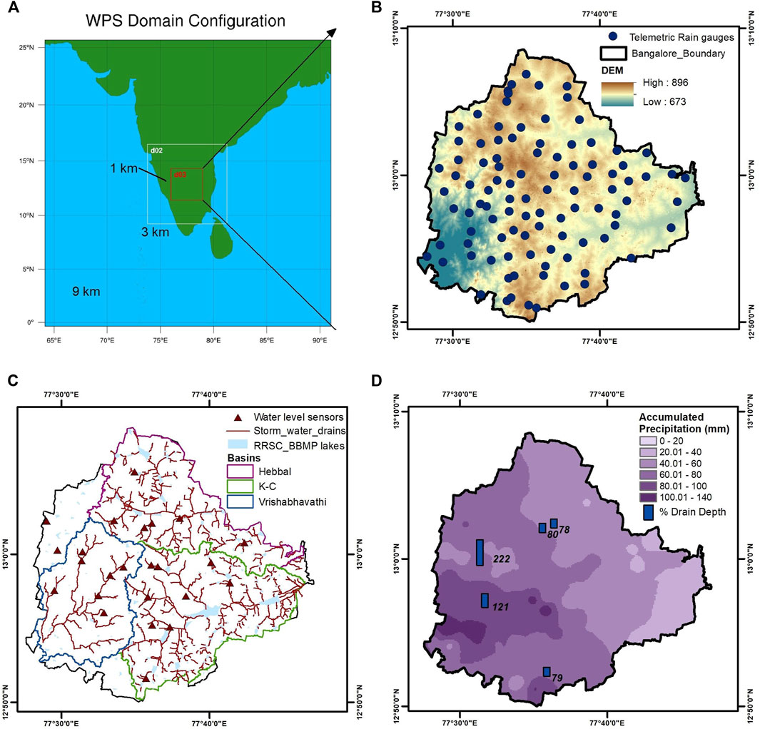
FIGURE 1. Study area and data used for development, calibration and validation of WRF and PCSWMM models. (A–D), WRF model domain configuration used for simulating extreme rainfall events over Bangalore city (A), Location of automatic rain gauges overlain over the digital elevation model (DEM) (B), Location of water level sensors with storm water drainage network, valley boundaries and lakes used for the development of the hydrological model (C) and Spatial map of observed rainfall for 20–21 October 2020 heavy rainfall event along with observed water levels represented as the percentage of flow depth with respect to drain depth (D).
Description of the Atmospheric Model
The atmospheric model used in the study is the WRF model which is used widely over the Indian region for creating short range rainfall forecasts. The WRF model version 3.6 (Skamarock et al., 2008) creates high resolution weather forecasts for a specific region. The dynamic core of the model solves the compressible non-hydrostatic Euler equations and the physical processes, which cannot be resolved to the model grid are represented empirically using parameterization schemes. The initial and boundary conditions required for the WRF model are generated from the Global Forecast System (GFS) which is a global weather forecast model maintained by the National Centre for Environmental Prediction (NCEP, 2015). The three hourly forecasts of climate variables at a horizontal resolution of 0.25° × 0.25° are given as an input to the model.
Description of the Hydrological Model
An urban flood model is useful in the assessment, study, and forecasting of flood conditions for reliable flood mitigation measures (Qi et al., 2021). In this study, the flood model used is the PCSWMM model (based on the United States Environmental Protection Agency’s SWMM5 model), which is a dynamic rainfall runoff model designed to simulate single and long-term events specifically for urban areas (Rossman, 2005; CHI, 2020). PCSWMM provides tools for 1D and 2D analysis of rainfall runoff process and also has the ability to model storm water source technologies (low impact development) to manage water quality and quantity. It facilitates modelling with the implementation of graphical user interface and GIS (Geographic Information System) enabled tools which make visualization and processing easier. PCSWMM can represent natural systems in urban regions as it can incorporate lakes and tanks using the storage unit feature. The model accounts for the hydrological processes that produce runoff from the urban catchments which include time-varying rainfall, evaporation, infiltration and helps in modelling the generation and transportation of runoff through a system of pipes, channels, and storage structures. The flowchart of the PCSWMM model methodology is shown in Supplementary Figure S1. The choice of hydrological modelling platform depends on the hydrological characteristics of the study areas and the data available. Bangalore is an inland catchment with a complex terrain with around 244 lakes acting as storage structures within the city and flooding is monitored via the water level in the storm water drains which were constructed based on the natural drainage within the city. The PCSWMM model is most suitable for modelling urban catchments with fast responses and connections between lakes and storm water drains. Hence, the PCSWMM modelling platform has been used for the study.
Coupling of Atmospheric and Hydrologic Model
WRF and PCSWMM models are one-way coupled with the rainfall forecasts from the high-resolution grid of the atmospheric model being forced into the hydrologic model to generate flood forecasts at predefined locations within the city. The forcing conditions which are generated at 18 UTC prior to the day of the event are selected for the model run. The coupled model cycle (as shown in Figure 2) is completed before 06 UTC of the event date.
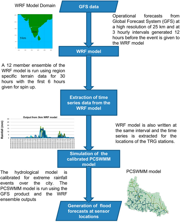
FIGURE 2. Flowchart representing the methodology of coupling of the atmospheric and hydrologic model. Operational GFS data is used to run the WRF model to generate high resolution rainfall forecasts. The data corresponding to the locations of the observed network is extracted and given as an input to the PCSWMM flood model to forecast water levels at critical sensor locations.
On test runs using different initial conditions, it is observed that the forecast boundary condition generated closest to the event gives a significantly improved result. After running the model, the rainfall variable is extracted from the WRF model grid at a high spatial and temporal resolution. A script using NCAR Command Language (NCL) and NetCDF Operators (NCO) commands are used to convert the coordinates and to extract time series files corresponding to grids nearest to the locations of the stations with the observed Automatic Rain Gauge (ARG) network (National Centers for Environmental Prediction, 2019; Zender, 2008; Zender, 2014). The time series of the rainfall forecast is provided as an input to the rain gauge locations using a Matlab code (Matlab, 2010). The spatial distribution of rainfall from these rain gauges within the sub-catchments are specified in the PCSWMM model using the Thiessen polygon (Akhter and Hewa, 2016) weighted method. After simulation, the flood model forecasts water levels at sensor locations distributed in the storm water drain network. Figure 2 shows the broad framework of model coupling.
Experiment Design Using the WRF Model
The WRF model comprises of three nested domains, with the outermost domain of 9 km resolution covering the Indian region with the adjacent oceans, the intermediate domain covering the southern part of India at a resolution of 3 km, and the innermost domain centered over the city of Bangalore with a resolution of 1 km as shown in Figure 1A. The WRF model takes 12 h to complete 30 h of simulation. Therefore, the forecast conditions generated by the Global Forecast Model (GFS) at 18 UTC the previous day is selected for the event. The model configuration used here has 38 vertical levels and the model top is kept at a constant pressure surface of 50 hPa. The details of the WRF model configuration are shown in Table 1.
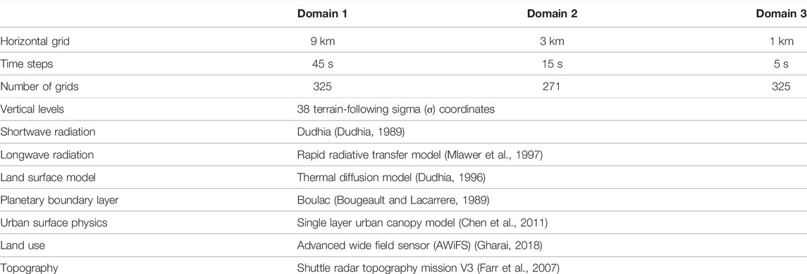
TABLE 1. WRF model configuration and physics scheme.
The land use land cover dataset in the United States Geological Survey (USGS) set of static data comprising of albedo, green fraction, land use land cover is replaced with a recent version of the dataset from the Indian Space Research Organization (ISRO) (2018-2019). The LULC data generated by the National Remote Sensing Centre (NRSC), ISRO, was derived from the Indian satellite IRS-P6, Advanced Wide Field Sensor (AWiFS) and is compatible with WRF pre-processing system. Many studies have demonstrated the improvement in the model outcomes, using this dataset over the Indian region (Kar et al., 2014; Sahoo et al., 2020a; Gupta et al., 2021), and also over the Bangalore region (Sahoo et al., 2020b). Navale and Singh (2020), Golzio et al. (2021) have demonstrated the significant impact of variation in topography on the fine scale pattern of rainfall generated by the WRF model over complex topography. The default topography dataset is the Global Multi-resolution Terrain Elevation Data (GMTED) (Danielson and Gesch, 2011) which has a resolution of 900 m (30 s).
This is replaced with the latest version of the Shuttle Radar Topography Mission (SRTM) dataset made available by the National Aeronautics and Space Administration (NASA). The NASA SRTM version 3 is a recently released version of the high resolution 30 m SRTM data which was void-filled using the GMTED 2010 data and the Advanced Spaceborne Thermal Emission and Reflection Radiometer (ASTER) Global Digital Elevation Model Version 3.
An ensemble of forecast scenarios is generated using a combination of convective and microphysics parameterization schemes that were used in the past studies over Bangalore city (Mohapatra et al., 2017; Bhimala et al., 2021; Rakesh et al., 2021; Sarkar and Himesh, 2021). The city having a complex terrain, may benefit from the high-resolution simulations as demonstrated by earlier studies. The simulations are carried out for each ensemble member, for 30 h and the model outcomes are recorded at a 15-min interval. The first 6 h are treated as spin-up and the 24 h corresponding to the rainfall event are used for analysis.
Studies have shown that certain processes that contribute to convection can only be captured when the resolution of the numerical model is below 2 km (Iriza et al., 2016). To understand this in detail, the rainfall forecasts obtained from both the domains—3 and 1 km are used in the study. It is also observed in the experimental test runs that different physics parameterization scheme combinations simulated the heavy rainfall event at both resolutions. The most commonly used convective parameterization schemes are the Kain Fritsch and the Betts Miller Janjic (BMJ) scheme. Kain Fritsch is a scheme that uses the Convective Available Potential Energy (CAPE) removal method to detect the onset of convection (Kain and Fritsch, 1993; Kain, 2004). BMJ scheme is an adjustment type scheme that generates deep and shallow convection (Janjić, 1994). The Grell Freitas scheme is a recently added convective scheme to the WRF model and has shown good performance over the Cauvery catchment region in Karnataka (Sarkar and Himesh, 2021). The three convective parameterization schemes chosen are based on the previous work done over Bangalore city by CSIR-4PI (Mohapatra et al., 2017; Bhimala et al., 2021; Rakesh et al., 2021; Sarkar and Himesh, 2021).
The microphysics (MP) scheme is responsible for heat and moisture flux within the atmosphere and gives the surface resolved rainfall. The WRF Single-Moment 6-class scheme (WSM6) is a scheme with ice, snow, and graupel processes suitable for high-resolution simulations. The WRF Double-Moment 6-class scheme (WDM6), has been developed by adding a double-moment treatment for the warm-rain process into the WSM6 scheme. Mohapatra et al. (2017) compared simulations of the WRF model for localised and non-localised urban extreme rainfall events over Bangalore city. The study concludes that the WRF model has a tendency to underestimate the magnitude of non-localized or uniformly distributed heavy rainfall events. This has been attributed to the incorrect treatment of cloud droplet size by the WSM6 scheme and the study suggests using the WDM6 scheme, as it has a better representation of physical processes.
Combinations using two microphysics schemes, three convective parameterization schemes, and two different resolutions result in a 12-member ensemble. The details of the ensemble are given in Table 2. In order to quantify the additional value provided by the rainfall forecasts from the WRF ensemble, the rainfall variable from the GFS is extracted. The time series for the locations of the ARG network is extracted from the corresponding grids of the GFS. The hydrological model is forced using the rainfall values from both the GFS and the WRF ensemble.
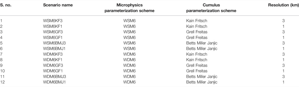
TABLE 2. List of physics combinations for the 12-member WRF ensemble.
Calibration and Validation of the PCSWMM Model
The development of the flood model for Bangalore city is completed using high density storm water drainage network, lakes data, and ARG network as shown in Figures 1B,C. The digital elevation model of 10 m resolution (as shown in Figure 1B) is procured from the National Remote Sensing Centre (NRSC), India. The details of the administrative boundaries and lakes used in the model are provided by Bruhat Bengaluru Mahanagara Palike (BBMP) and Regional Remote Sensing Centre (RRSC) (Hebbar et al., 2018) as shown in Figure 1C. The percentage imperviousness of sub-catchments is calculated using the Land Use Land Cover (LULC) map for the year 2020 provided by the Bengaluru Development Authority (BDA). The details of the input data to the PCSWMM model are given in Supplementary Table S1. The datasets for the model setup., viz., nodes, drains, storage tanks, ARG locations, and sub-catchments are processed, connected and imported from ArcGIS (version 10.3) to PCSWMM. The runoff is computed at the sub-catchment level after accounting for various losses and the flow from the sub-catchment outlets is routed kinematically through storm water drainage channels. More details on urban flood model development for Bangalore city are given in Mujumdar et al. (2021).
The three valleys are independent of each other with different outlet points and in their response to rainfall events. Hence the valleys are calibrated and validated separately for different rainfall events. The observed water level data at some sensors because of blockage to the flow, shows fluctuations and rise in water depth irrespective of rainfall. The water level sensors are selected for calibration and validation based on the availability of the observed water level data with no unaccounted flow and continuity of the data in the time period. The PCSWMM model developed over Bangalore city is calibrated using a recent heavy rainfall event that occurred on 8, 9 September 2020 (Supplementary Figure S2A).
The model output is verified against water level data at a high temporal resolution of 15 min. The parameters considered for the calibration of the model include sub-catchment properties which are width, Manning’s roughness coefficient, and percentage imperviousness, properties of the storm water network, viz., the slope and roughness coefficient of the conduits. The model is further validated for a heavy rainfall event on 5, 6 November, 2020 (Supplementary Figure S2B). Calibration and validation of the model is demonstrated here for a sensor located in the Hebbal valley, a catchment towards the northern side of Bangalore city. The performance indices for the calibration and validation of the model are as shown in Supplementary Table S2. The model is seen to perform well and is used to generate flood water levels for the rainfall forecasts from the WRF model ensemble and the GFS.
Event Description
Bangalore city receives rainfall from both south-west (from June to September) and north-east (from October to December) monsoon. The model coupling framework discussed (Figure 2), is used to simulate extreme events over the region for the monsoons of years 2020 and 2021(Supplementary Figures S3–S6). An extreme rainfall event that occurred on 20 and 21 October 2020, is selected for a detailed demonstration of this framework. The spatial pattern of this particular event had spatial characteristics similar to the mean return levels of annual maximum precipitation with a 10-years return period (Supplementary Figure S7).
The southwest monsoon in the year 2020 was prolonged due to unseasonal weather systems that occurred in the Arabian sea and the Bay of Bengal (IMD, 2020). The onset of the north east monsoon season was delayed by 3 weeks. The heavy rainfall event marked the end of the southwest monsoon of 2020 over Bangalore city. This event occurred between the depression over the Arabian Sea (17–19 October 2020) and the depression over Bay of Bengal (22–24 October 2020).
The city received heavy rainfall throughout on 20 and 21 October 2020 and a daily rainfall maximum of 124.5 mm was observed at Kengeri station in Raja Rajeshwari Nagar located in the Vrishabhavathi valley (Supplementary Figure S8). In the event of a flood, water levels at the sensors that exceed 75% of the drain depth are assumed to be critical as per the alert system followed by the urban flood model during flooding (Mujumdar et al., 2021). The five sensors which were identified as critical at the time of the observed event is then selected and studied here. The maximum water level from these sensors is expressed in terms of the percentage of drain depth which shows the level of water relative to the drain depth at each location. The details of the water level sensors such as location, depth of drain, and observed water level data for the 20–21 October 2020 event at critical sensors (>75% drain depth) are given in Supplementary Table S3 (Supplementary Figure S9).
Performance Indices for Rainfall Forecasts
The skill of the WRF model presented here is evaluated by comparing the simulated and observed rainfall at a high resolution of 15 min. The performance indices are used to analyze spatial and temporal errors across the observational network. To calculate categorical indices, the variable values are considered in a non-probabilistic manner. Categorical statistics are computed from the elements in the contingency table (Wilks, 2006) as shown in Table 3. Hits refer specifically to those grids which show rainfall. For a sample threshold value of 40–60 mm, the values are calculated accordingly. If the observed grid is showing a value between 40 and 60 mm and the corresponding model grid is showing a value in the same range, it is a Hit.

TABLE 3. Contingency table for the calculation of categorical indices.
If the model grid is showing a value lesser than 40 mm it is a Miss. If the model grid is showing a value greater than 60 mm it is a false alarm. If the value in the observed grid doesn’t fall within this range and the same is calculated for the model grid, then it is a correct negative.
The Critical Success Index (CSI), also known as the Threat Score, describes the overall skill of the simulation relative to the observation. The CSI value ranges from 0 to 1, where 0 indicates no skill and 1 indicates perfect skill. It measures the fraction of observed and forecast events that were correctly predicted. It does not distinguish the source of the forecast error. It is described as shown in Eq. 1.
Some additional indices that are calculated using the contingency table are accuracy, bias score (BS), probability of detection (POD) and Hiedke Skill Score (HSS) the details of which are provided in the supplementary document (Supplementary Table S4).
The categorical indices are obtained based on the spatial distribution patterns from the observed rainfall. Continuous and categorical indices are calculated in comparison with the observed data and the ensemble members performing better are identified. The rainfall time series for each station is provided as an input to the PCSWMM model and the model is run with the best performing subset of the WRF ensemble. The 3-h time series from the GFS were also given as an input to the PCSWMM model. The water levels at various locations are compared and analyzed for performance evaluation against the observed data.
Results and Discusssion
The performance of the WRF ensemble is assessed for the selected event using categorical indices. The best performing members are then selected as a subset and used in hydrological modelling. The additional value from the high resolution WRF model output (3 and 1 km at 15 min intervals) as compared to the GFS data (25 km at three hourly intervals) is quantified in this section.
Verification of Spatial Distribution
gridded data is plotted using the ArcGIS software after accumulating rainfall, 08:30 a.m. to 21 October 08:30 a.m. 2020 (ESRI, 2020). It can be observed that the microphysics scheme plays a significant role in the amount of rainfall simulated from Figure 3. Scenarios using the WSM6 scheme (Figures 3A–F) have forecasted a higher quantity of rainfall as compared to those with WDM6 (Figures 3G–L). The single-moment microphysics scheme predicts the total mass concentration of hydrometeors (liquid or solid water particles that may be suspended or fall through the atmosphere) whereas double moment schemes include the prediction of total number concentration (number of particles per volume). Cloud Condensation Nuclei (CCN) and number concentration are the two additional variables predicted in the double moment scheme. This scheme is selected because it has a better physical representation of the processes. However, some studies have shown that in certain regions the simulation of CCN has resulted in an overall decrease in the rainfall quantity (Li et al., 2008). Also, the performance of the double moment scheme is dependent on the accuracy of a large number of microphysics processes than the single moment scheme (Lim and Hong, 2010).
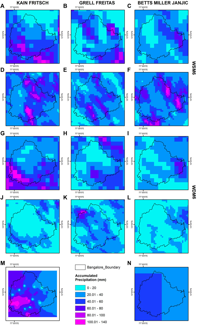
FIGURE 3. Spatial distribution of 24 h accumulated rainfall (mm) from WRF ensemble, Global Forecast System (GFS) data and observed rainfall. (A–N), Spatial distribution of 24 h accumulated rainfall (mm) from WRF ensemble simulations WSM6KF3 (A), WSM6GF3 (B), WSM6BMJ3 (C), WSM6KF1 (D), WSM6GF1 (E), WSM6BMJ1 (F), WDM6KF3 (G), WDM6GF3 (H), WDM6BMJ3 (I), WDM6KF1 (J), WDM6GF1 (K), WDM6BMJ1 (L), the Global Forecast System (GFS) data (N), and observed (M), over the Bangalore city for the period 0300 UTC 20 October to 0300 UTC 21 October 2020. The heavy rainfall quantities (>60 mm/day) is well represented by the WRF ensemble and it can be seen from (A–L) that the extreme rainfall pattern is reflected in the WRF ensemble output as compared to the GFS. The three columns correspond to the three convective parameterization schemes selected for the study—Kain Fritsch, Grell Freitas, and Betts Miller Janjic. The first two rows show the results from WSM6 microphysics schemes and the next two rows present the results from WDM6.
The convective parameterization (CP) scheme details the sub-grid processes associated with convective clouds and operates only on individual columns where the scheme is triggered and provides the convective component of rainfall. Among the convective schemes selected for the study, Kain Fritsch gives better spatial representation in comparison to the observed rainfall (Figures 3A,D,G,K). The location of the event is well simulated by the Kain Fritsch scheme across domains and microphysics schemes.
The comparison of results for 1 and 3 km shows no significant pattern to determine the better performance among the two domains. The 1 km domain performs better for the WSM6 microphysics scheme whereas, the 3 km domain performs better for the WDM6 scheme. A similar observation was made in a comparison study by the Korean Meteorological Agency which observes that both WSM6 and WDM6 underestimate convective events in spite of WDM6 predicting realistic rain drop size and relative humidity due to a dependence on grid resolution (Min et al., 2015). However, for a combination of certain physics schemes - WSM6KF (Figures 3A,D) and WDM6GF (Figures 3H,K), both the domains offer a fair representation of the spatial pattern. More events need to be considered in order to understand the combined impact of grid resolution and microphysics schemes. Out of the 12 forecast scenarios, 10 indicate the occurrence of a heavy rainfall event for the given time period within the city (Figures 3A–I,K).
Categorical Indices
The categorical indices are calculated for the 12 simulations created for the heavy rainfall event that occurred on 20–21 October 2020. For each simulation, the indices are calculated for different rainfall thresholds—20, 40, 60, 80, 100, and 140 mm as shown in Supplementary Figures S10A,B. Capturing the location of the rainfall, plays an important role in flood forecast and therefore the ensemble members which capture the location of the rainfall range gives higher CSI values. For example, the rainfall in the range of 40–60 mm lies in the central part of the city and the members WSM6GF1, WSM6BMJ3, and WSM6KF1 capture it with the highest CSI values (Supplementary Figure S10B). The heavy rainfall range (>60 mm) for this event occurs towards the south western side of Bangalore city, and although there is a general underestimation from the ensemble, some scenarios, viz., WSM6KF3, WSM6KF1, and WDM6KF3 predict the location accurately (Figures 3A,D,J).
The WSM6KF3 configuration of the WRF ensemble is also validated across four heavy rainfall events from the monsoons of 2020 and 2021—September 8–9, October 20–21 for the year 2020 and November 4–5, October 11–12 for the year 2021. The spatial verification and categorical metrics calculated across these events for different rainfall thresholds are included in the supplementary material (Supplementary Figures S3–S6, S11; Supplementary Tables S4, S5). On an average, the model setup has a better performance than a random/chance forecast for a rainfall threshold of 60 mm as can be seen by the positive value of Hiedke Skill Score (Supplementary Figure S11). Based on the spatial distribution of rainfall and categorical indices, the ensemble members with better model performance are identified and used in the flood forecast model. The members identified to be given as an input to the hydrological models are—WSM6KF3, WSM6KF1, WSM6GF3, WSM6GF1, WDM6KF3, and WSM6BMJ3. The time series of this subset is further verified at locations adjacent to the critical water level sensors in the hydrological model.
Verification of Temporal Distribution
The 15-min time series data corresponding to the automatic rain gauges is extracted from the above-mentioned WRF ensemble subset and is provided as an input to the PCSWMM model. The time series for six ensemble members at three critical locations (one representative of each valley) are examined here as shown in Figure 4. The GFS data extracted for the location is also shown in Figure 4. It can be seen for all valleys, that the 15-min maximum value of the observed time series is captured.
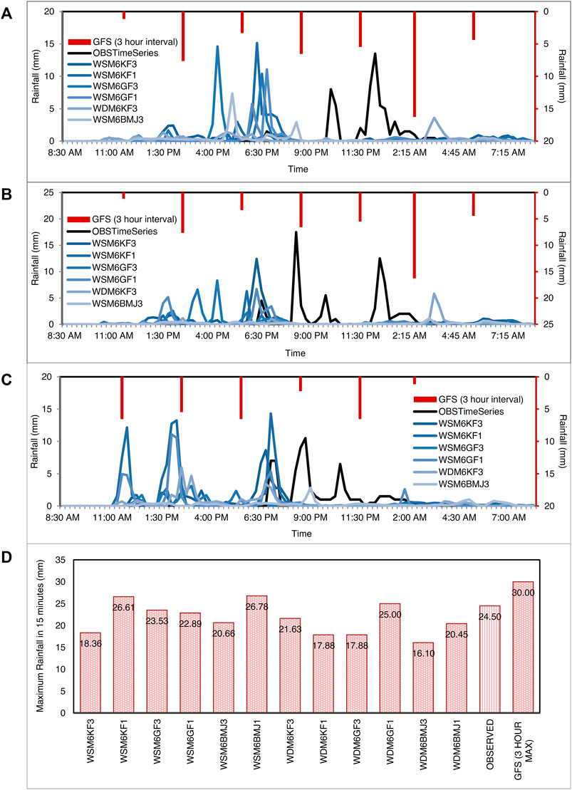
FIGURE 4. Comparison of rainfall time series from the selected forecast scenarios for rain gauge locations. (A–C), Comparison of rainfall time series from the WRF forecasts, GFS forecasts and Observed rainfall for ARG locations in Koramangala-Chellaghatta valley (A), Vrishabhavathi valley (B), and Hebbal valley (C). (D), Comparison of 15-min maximum rainfall from each member of the ensemble with the 15-min maximum value from observed ARG network. The WRF ensemble is able to capture the intensities of the event as compared to the GFS.
For Koramangala-Chellaghatta (KC) valley, maximum values and the temporal patterns of rainfall at 15 min are captured by the ensemble member, for Vrishabhavathi (VV) valley the patterns are captured with lesser intensity and in Hebbal valley, a slight overestimation is noted as shown in Figures 4A–C. The GFS data (red bar graphs shown on the inverted axis in Figures 4A–C) consistently underestimates the daily rainfall value at all three locations and the timing of the peak occurs after the rainfall event at some locations.
The WRF model is able to capture the intensities of the rainfall albeit with a temporal shift. This could be due to the fact that the single layer urban canopy physics option used may not capture the heat exchanges that happen within the city. Opting for a multi-layer urban canopy model and incorporating detailed representation of urban land use classes in future studies may improve the timing of the prediction (Holt and Pullen, 2007; Salamanca et al., 2011; Jandaghian and Berardi, 2020). The WRF model output is captured at every 15 min as against the 3-h time interval of the input GFS data. The 15-min maximum value for the rainfall forecast from each WRF ensemble member is compared against the observed data. Even the lower performing members of the ensemble, WDM6KF1, and WDM6BMJ1 based on the spatial verification shown in Figures 3K,L have captured a maximum value of 17.88 and 25 mm respectively, as compared to the observed value of 24 mm.
Most ensemble members capture the 15-min maxima with a variation of not more than 10 mm. This implies that irrespective of the spatial and temporal displacements of the simulated rainfall, the maximum intensity is fairly well captured by the WRF model ensemble. The maximum from the GFS is 30 mm in a 3-h interval which is very low in comparison to the values from the WRF ensemble. From this section, it can be concluded that three hourly rainfall forecasts from GFS fail to capture the temporal variability and intensity of the observed rainfall.
Comparison of PCSWMM Model Output
The WRF ensemble members are selected based on their ability to simulate the spatial distribution and location of heavy rainfall (>60 mm/day), and the forecasted rainfall is given as inputs to the hydrological model. Prediction of water levels in urban flooding situations requires accurate sub-hourly intensity/values of rainfall to be given as an input to the flood models. The data extracted at rain gauge locations from the nearest grids in the WRF model is given as input to the PCSWMM model. The spatial plot of the PCSWMM input data is shown in Figure 5. The spatial distribution of rainfall is improved by downscaling the GFS data as visible in Figures 5A–H in terms of extent and intensity, and similar improvement can be observed for water level forecasts.
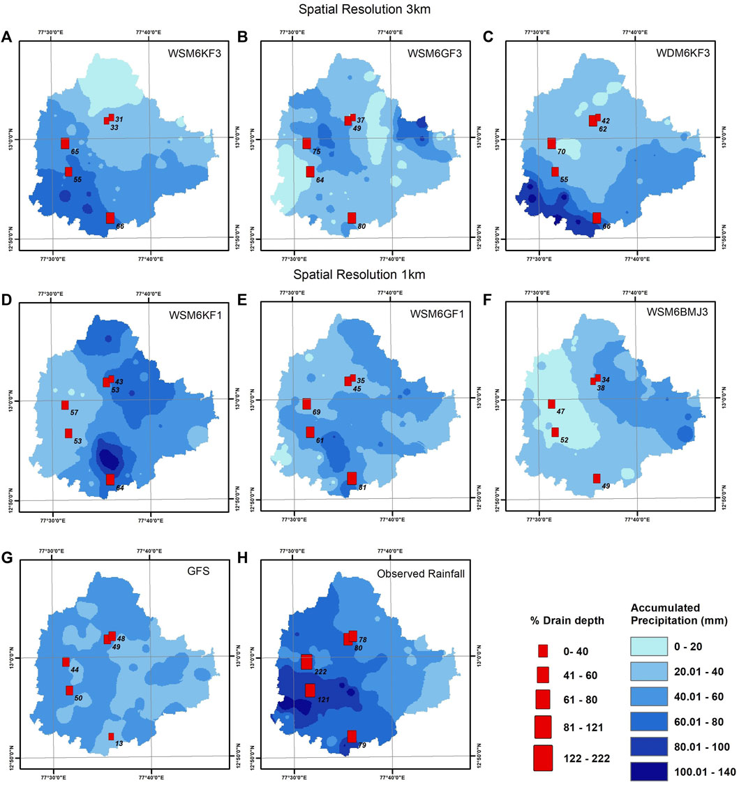
FIGURE 5. Rainfall forecasts from WRF ensemble members and GFS forecast and the corresponding water level forecasts. (A–F), Spatial variability in rainfall and corresponding flood forecasts from WRF ensemble member WSM6KF3 (A), WSM6GF3 (B), WDM6KF3 (C), WSM6KF1 (D), WSM6GF1 (E), WSM6BMJ3 (F), (G,H) Spatial variation in rainfall and corresponding flood forecasts from GFS (G), and Observed ARGs (H). The red boxes indicate the forecasted water levels at critical locations by the model represented as percentage of drain depth occupied by water. The water level forecasts show similarity with the observed water levels which are better than the forecasts using GFS.
The critical water level sensors in Vrishabhavathi, Koramangala-Chellaghatta, and Hebbal valley are selected for the analysis based on the observed water level depth during the storm event (>75% of drain depth). The plots also show the outputs from PCSWMM for these sensor locations across Bangalore city (Figures 5A–G) and the peak water level depths at those locations are expressed in terms of the percentage of the drain depth covered. The PCSWMM model simulation outputs for the three hourly rainfall time series from the GFS data are also shown in Figure 5G.
The spatial distribution of the rainfall forecasts has a significant impact on the water level peak forecasts as can be seen from Figures 5A–F. For Koramangala-Chellaghatta and Hebbal valley, the WRF model forecasts are performing better than the GFS data forecasts. For the critical sensors in Vrishabhavathi valley, which had the highest recorded water levels (exceeds the drain depth by 122 and 21%), the values are underestimated by both the WRF ensemble and GFS data. The flood model responds well to all sources of rainfall input (Observed, WRF ensemble, and GFS data) and the variation in the water level correlates with rainfall intensities. The error in predicting the location of the heavy rainfall threshold (above 60 mm/day) impacts the forecasts of the flooding locations from the hydrological model.
It can be observed that water level peaks are being captured at certain locations in spite of a general underestimation in the rainfall forecasts. This can be attributed to the fact that the sub hourly rainfall intensity which is a strong indicator of the extremity of the event is captured to a larger extent by the WRF downscaled forecasts. It can be observed in Figure 4C that the 15-min maximum rainfall from observed sensors which is 24 mm is fairly captured by all members of the ensemble.
A spatial shift in the simulated rainfall can be observed in certain ensemble members towards the southern side of Bangalore (shown Figures 5C,D), which is reflected in the simulated water depths. The spatial distribution of rainfall has improved to a greater extent using the WRF ensemble forecasts, Also, the forecasted water levels are closer to the observed data and higher than the GFS data forecasts.
Verification of Flood Forecasts From PCSWMM
The high spatial and temporal intensity of the urban flood that occurred following the heavy rainfall event on 20–21 October 2020 is captured fairly by the PCSWMM model. The observed rainfall data from the ARGs is given as an input and the flood model output (Input_ARG_Rainfall) is compared with the water level sensor data and flood forecast values from the WRF ensemble and GFS data as shown in Figures 6A,B. It can be observed from Figure 6A the water level forecast from the WRF ensemble provides a good indication of high water levels and shows a high variability when compared with forecasts from the GFS data as shown in Figures 6A,B. Similar result can be observed for sensors in Vrishabhavathi valley (Supplementary Table S6). From extensive field visits and ground scenario comparisons, it is observed that certain obstructions in the form of debris from sewage flow, including solid waste and tree/plant growth, cause the water in the storm water drains to rise resulting in outliers in the observed water level sensors data as shown in Figure 6B. It can be seen from Figure 6B, that the flood forecast is not able to capture the peak value (2.2 m) which maybe a result of external factors and not the rainfall event. Excluding the outlier value, the maximum water level (0.9 m) is reflected in the flood forecasts generated using the WRF ensemble.

FIGURE 6. Comparison of water level at critical water level sensor locations. (A,B), Comparison of forecasted water level using WRF ensemble forecasts, GFS forecasts and observed rainfall with observed water levels at water level sensor location in Vrishabhavathi valley (A) and Koramangala-Chellaghatta valley (B) at 15-min interval. The water level is captured fairly using WRF forecasts than GFS forecasts. (C,D), comparison of forecasted water levels from WRF ensemble members(3 h averaged) and GFS forecasts at three hourly intervals at water level sensor location in Vrishabhavathi valley (C), and Koramangala-Chellaghatta valley (D).
Based on observations made for Vrishabhavathi Valley, it can be observed from Supplementary Table S6, that the model performs well in predicting water level peaks for all valleys. As shown in Supplementary Table S6, 50 and 16.7% of the ensemble members indicate flooding (>75% drain depth) for Koramangala-Chellagatta and Vrishabhavathi valley respectively which is useful for early warning and disaster preparedness. The average percentage drain depth obtained from the flood forecast using WRF ensemble is 63 and 70 for Vrishabhavathi and Koramangala-Chellagatta valley, respectively.
The WRF forced PCSWMM model output was further averaged to 3 h to match with the resolution of the GFS data The results shown in Figures 6C,D, indicate that the WRF ensemble captures the variability with a slight underestimation in the flood peak. Flooding in urban areas is majorly caused by high-intensity short duration rainfall which leads to saturation of the available pervious area and overwhelming of the drainage capacity. When using the forecast from the GFS data as rainfall input, with an interval of 3 h most of the rainfall infiltrates and the soil is not saturated enough to produce an overland flow that can contribute to an increase in the water level. This results in the water levels remaining unchanged throughout the hydrological model run (Figure 6). The high-resolution rainfall forecasts from the WRF ensemble produce the flood peaks more effectively than the GFS data as shown in Figure 7. The hydrological model simulation when forced with global forecast at 3-h intervals, is not able to accurately represent the hydrology specially of an urban area and thus highly underestimates the flood magnitude.
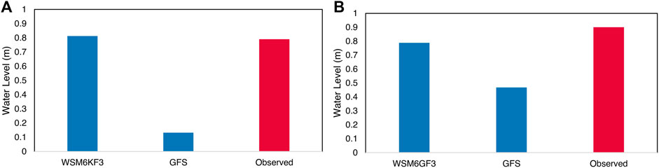
FIGURE 7. Comparison of maximum water level at critical water level sensor locations. (A,B), Comparison of water level between maximum value from WRF ensemble forecast, GFS forecast and observed data at sensor location in Koramangala-Chellaghatta valley (A), and Vrishabhavathi valley (B). The bias between the WRF ensemble and the GFS is 0.68 and 0.32 m. The flood maximum value is predicted by the WRF ensemble at both locations.
Conclusion
The rising number of extreme events in Indian cities is a serious concern with the high population density and unplanned growth, making them suffer huge economic losses in the aftermath of such an event. As per the recent IPCC reports, the increase in the global temperature is bound to bring about unprecedented changes which cannot be predicted by analyzing historical data. The impact of recent urban floods highlights the requirement for the development of a high-resolution flood forecasting system for Indian cities. The nature of the urban flood demands a system built using high resolution data to capture the sub-hourly intensities occurring for short durations, as, such rainfall events are known to cause extensive damage. The city of Bangalore has a high-density network of automatic rain gauges and water level sensors. The data is made available at a 15-min temporal resolution; hence the city is used as a case study to evaluate a real time flood forecasting system. In this context, the real time forecast data at a resolution of 25 km from the Global Forecast System model—is used to as a boundary condition to drive the WRF model. As Bangalore covers an area of 765 km2, climate data at 25 km maybe insufficient to resolve interactions with local topography and adequately forecast convective systems that may cause extreme rainfall events and urban flooding as a consequence. Hence, a popularly used RCM, the WRF model, is used to dynamically downscale real time climate information to a high resolution of 3 and 1 km. As WRF model outputs contain some uncertainty associated with the complexity of the rainfall generation process, a combination of 12 model configurations, with different physics schemes are used for the experiment.
The PCSWMM modelling platform is used to study the urban hydrology, using high resolution datasets to obtain water level observations in open channel drains. The model was calibrated, validated, and run for real time scenarios and have been able to effectively capture the points of flooding for the selected extreme events. This urban flood model is used for flood forecasting by using rainfall data from the WRF model and GFS data. The additional value brought about by using the WRF model is evaluated by comparing the flood forecasts from GFS data with the observed.
The present study reveals that the high-resolution WRF model is able to provide additional value in terms of characteristics of the rainfall pattern and sufficient variability in the water level pattern as compared to the 25 km GFS data. The accumulated rainfall and its location are found to be sensitive to the choice of convective and microphysics parameterization schemes. Model simulated rainfall is noted to be closer to the observed rainfall in the case when the microphysics scheme is WSM6 and the convective parameterization scheme is Kain Fritsch.
Ten out of the twelve members of the WRF ensemble, forecast an extreme rainfall event within the city. The GFS data shows a rainfall event but fails to capture any rainfall above 60 mm/day which is the threshold for flooding in Bangalore city (Mohapatra et al., 2017). Six out of twelve members are successful in capturing the location and spatial distribution of the event and are used as an input for the calibrated PCSWMM model (Supplementary Figure S2).
The spatial and temporal resolution of the rainfall input plays an important role in the urban flood event analysis. The dense spatial and temporal network used for verification of the performance of the forecasting framework is a novelty of the work. It can be seen that the flood model outputs using the WRF ensemble data have more variability as compared to the runs using the GFS data as an input. The inability to capture the extreme rainfall features and the coarse temporal resolution of the GFS data has caused the water level output to be both spatially and temporally unvaried. The WRF ensemble aids in the model performance for flood forecasts with the ensemble water level peaks being much closer to the observed than GFS data (Figure 7). The flood peak appears 6–8 h in advance as compared to the observed which may be due to inadequate representation of urban heat island effect within the model (Paul et al., 2018).
The study demonstrates the first ever integrated application of a high-resolution numerical weather model coupled with a detailed hydrological model to capture a recent urban flood event over an Indian city. The urban catchment considered for the study is a lake based inland catchment and can serve as a model for other cities with similar urban hydrology. While the Bangalore city is a highly gauged or data rich study area that facilitates urban flood forecasting studies, the study framework can be adaptable for any city by giving inputs that reflect extreme rainfall events. The best performing member of the modelling framework (WSM6KF3) has been tested for various events and the performance across events have been included in the supplementary section for the sake of brevity (Supplementary Figures S3–S6, S11, Supplementary Tables S4, S5). The WSM6KF3 member has been tested for four heavy rainfall events from the monsoons of 2020 and 2021—September 8, 9; October 20, 21; 2020: November 4, 5; October 10, 11; 2021. The combined categorical indices have been added to the supplementary material (Supplementary Figure S11). On an average, the model setup has a better performance than a random/chance forecast for rainfall threshold above 60 mm as can be seen by the positive value of Hiedke Skill Score (Supplementary Figure S11A).
The WRF model ensemble is being improved continuously to reduce inconsistencies and errors in the initial conditions. The current physics ensemble selected for the study needs to be calibrated further in order to develop an ensemble with each member equally likely to predict a convective storm one to 3 days in advance. The accuracy of the ensemble can be further improved by assimilation of the observed network data. The one-way coupled framework has certain limitations as the feedback of surface hydrology variables such as lateral water flow and soil moisture to the atmospheric model are not considered. The lack of a two-way feedback mechanism also leads to the separation of the rainfall process from the land surface hydrological processes.
The modelling framework is designed to generate short range forecasts for the city of Bangalore. Continuous assessment of the operational runs of this framework can be used to develop medium range and long-range flood forecasts. Operational forecasts from the flood forecasting framework aids in building climate resilience for the city if and when these urban feedbacks are considered into regional planning processes (Gonzalez et al., 2021). The accuracy of the modelling framework can be further improved to include future sources of climate data—localised climate zones, data assimilation, higher resolution LULC and DEM. It can also be utilised for future climate scenarios if uncertainties from corresponding future land use land cover prediction datasets that will be used in the hydrological models is quantified.
Data Availability Statement
The data analyzed in this study is subject to the following licenses/restrictions: High resolution observation data provided by the Karnataka State Natural Disaster Monitoring Center is available on request basis and is not publicly accessible. Data provided by local government bodies are classified and is not available on a public platform. Requests to access these datasets should be directed to Director, KSNDMC, Government of Karnataka (E-mail: ZGlyZWN0b3JAa3NuZG1jLm9yZw==).
Author Contributions
PM designed the concept, edited and proofread the manuscript. SD carried out the development, pre-processing and simulation of WRF model, post-processing of WRF results and writing manuscript. NS and LP worked on development, simulation and data analysis of hydrological model, post-processing of WRF results, preparation of results, editing and formatting manuscript.
Funding
Ministry of Electronics and Information Technology (MeITy), under the National Supercomputing Mission program of Government of India, through the following project: “Urban Modelling: Development of Multi-sectorial Simulation Lab and Science-Based Decision Support Framework to Address Urban Environment Issues” (Sanction Number MeitY/R&D/HPC/2(1)/2014).
Conflict of Interest
The authors declare that the research was conducted in the absence of any commercial or financial relationships that could be construed as a potential conflict of interest.
Publisher’s Note
All claims expressed in this article are solely those of the authors and do not necessarily represent those of their affiliated organizations, or those of the publisher, the editors and the reviewers. Any product that may be evaluated in this article, or claim that may be made by its manufacturer, is not guaranteed or endorsed by the publisher.
Acknowledgments
The authors acknowledge the financial support from Centre for Development of Advanced Computing (CDAC), on behalf of the Ministry of Electronics and Information Technology (MeITy), under the National Supercomputing Mission program of Government of India, through the following project: “Urban Modelling: Development of Multi-sectorial Simulation Lab and Science-Based Decision Support Framework to Address Urban Environment Issues” (Sanction Number MeitY/R&D/HPC/2(1)/2014). The authors would like to thank the Karnataka State Natural Disaster Monitoring Centre (KSNDMC), Bruhat Bengaluru Mahanagara Palike (BBMP), Bengaluru Development Authority (BDA), National Remote Sensing Centre (NRSC), Regional Remote Sensing Centre (RRSC), India Meteorological Department (IMD), and, National Aeronautics and Space Administration (NASA), for providing the high-resolution data used in this study. The authors are thankful to Pankaj Dey for his help in proofreading the manuscript.
Supplementary Material
The Supplementary Material for this article can be found online at: https://www.frontiersin.org/articles/10.3389/feart.2022.883842/full#supplementary-material
References
Akhter, M., and Hewa, G. (2016). The Use of PCSWMM for Assessing the Impacts of Land Use Changes on Hydrological Responses and Performance of WSUD in Managing the Impacts at Myponga Catchment, South Australia. Water 8, 511. doi:10.3390/w8110511
Allen, M. R., Dube, O. P., Solecki, W., Aragón-Durand, F., Cramer, W., Humphreys, S., et al. (2018). Framing and Context. In: Global Warming of 1.5°C. An IPCC Special Report on the Impacts of Global Warming of 1.5°C above Pre-industrial Levels and Related Global Greenhouse Gas Emission Pathways, in the Context of Strengthening the Global Response to the Threat of Climate Change, Sustainable Development, and Efforts to Eradicate Poverty. Editors V. Masson-Delmotte, P. Zhai, H.-O. Pörtner, D. Roberts, J. Skea, P.R. Shuklaet al. IPCC. https://www.ipcc.ch/site/assets/uploads/sites/2/2019/06/SR15_Full_Report_High_Res.pdf.
Arnold, D., Morton, D., Schicker, I., Seibert, P., Rotach, M. W., Horvath, K., et al. (2012). Issues in High-Resolution Atmospheric Modeling in Complex Topography - the HiRCoT Workshop. Hrvat. Meteoroloski Cas. 47 (47), 3–11. https://meteo.boku.ac.at/report/BOKU-Met_Report_21_online.pdf.
Asghar, M. R., Ushiyama, T., Riaz, M., and Miyamoto, M. (2019). Flood and Inundation Forecasting in the Sparsely Gauged Transboundary Chenab River Basin Using Satellite Rain and Coupling Meteorological and Hydrological Models. J. Hydrometeorol. 20 (12), 2315–2330. doi:10.1175/JHM-D-18-0226.1
Awol, F. S., Coulibaly, P., and Tsanis, I. (2021). Identification of Combined Hydrological Models and Numerical Weather Predictions for Enhanced Flood Forecasting in a Semiurban Watershed. J. Hydrol. Eng. 26 (1), 04020057. doi:10.1061/(asce)he.1943-5584.0002018
Bhimala, K. R., Gouda, K. C., and Himesh, S. (2021). Evaluating the Spatial Distribution of WRF-Simulated Rainfall, 2-m Air Temperature, and 2-m Relative Humidity over the Urban Region of Bangalore, India. Pure Appl. Geophys. 178 (3), 1105–1120. doi:10.1007/s00024-021-02676-4
Bougeault, P., and Lacarrere, P. (1989). Parameterization of Orography-Induced Turbulence in a Mesobeta-Scale. Mon. Weather Rev. 117, 1872–1890.
Chawla, I., and Mujumdar, P. P. (2015). Isolating the Impacts of Land Use and Climate Change on Streamflow. Hydrol. Earth Syst. Sci. 19, 3633–3651. doi:10.5194/hess-19-3633-2015
Chawla, I., Osuri, K. K., Mujumdar, P. P., and Niyogi, D. (2018). Assessment of the Weather Research and Forecasting (WRF) Model for Simulation of Extreme Rainfall Events in the Upper Ganga Basin. Hydrol. Earth Syst. Sci. 22, 1095–1117. doi:10.5194/hess-22-1095-2018
Chen, F., Kusaka, H., Bornstein, R., Ching, J., Grimmond, C. S. B., Grossman-Clarke, S., et al. (2011). The Integrated WRF/Urban Modelling System: Development, Evaluation, and Applications to Urban Environmental Problems. Int. J. Climatol. 31 (2), 273–288. doi:10.1002/joc.2158
Chevuturi, A., Dimri, A. P., Das, S., Kumar, A., and Niyogi, D. (2015). Numerical Simulation of an Intense Precipitation Event over Rudraprayag in the Central Himalayas during 13-14 September 2012. J. Earth Syst. Sci. 124, 1545–1561. doi:10.1007/s12040-015-0622-5
CHI (Computational Hydraulics International) (2020). PCSWMM Professional 2D Version: 7.3.3095, Guelph, Ontario, Canada. [Online]. Available: www.chiwater.com (Accessed August 08, 2021).
Clark, P., Roberts, N., Lean, H., Ballard, S. P., and Charlton-Perez, C. (2016). Convection-permitting Models: A Step-Change in Rainfall Forecasting. Mater. Apps. 23 (2), 165–181. doi:10.1002/met.1538
Danielson, J. J., and Gesch, D. B. (2011). “Global Multi-Resolution Terrain Elevation Data 2010 (GMTED2010),” in Open-File Report. doi:10.3133/ofr20111073
Dhote, P. R., Thakur, P. K., Aggarwal, S. P., Sharma, V. C., Garg, V., Nikam, B. R., et al. (2018). Experimental Flood Early Warning System in Parts of Beas Basin Using Integration of Weather Forecasting, Hydrological and Hydrodynamic Models. Int. Arch. Photogramm. Remote Sens. Spat. Inf. Sci. XLII-5 (5), 221–225. doi:10.5194/isprs-archives-XLII-5-221-2018
Dudhia, J. (1989). Numerical Study of Convection Observed During the Winter Monsoon Experiment Using a Mesoscale Two-Dimensional Model. J. Atmos. Sci. 46, 3077–3107.
Evans, J. P., Ekström, M., and Ji, F. (2012). Evaluating the Performance of a WRF Physics Ensemble over South-East Australia. Clim. Dyn. 39, 1241–1258. doi:10.1007/s00382-011-1244-5
Farr, T. G., Rosen, P. A., Caro, E., Crippen, R., Duren, R., Hensley, S., et al. (2007). The Shuttle Radar Topography Mission. Rev. Geophys. 45 (2). doi:10.1029/2005RG000183
Gharai, B. (2014). IRS-P6 AWiFS Derived Gridded Land Use/Land Cover Data Compatible to Mesoscale Models (MM5 and WRF) over Indian Region. NRSC Technical Document No. NRSC-ECSA-ACSG-OCT-2014-TR-651, 1–11. Available at: http://bhuvan.nrsc.gov.in.
Ghosh, M., Karmakar, S., and Ghosh, S. (2022). “Flood Modelling for an Urban Indian Catchment: Challenges and Way Forward,” in Climate Change and Water Security. Lecture Notes in Civil Engineering. Editors S. Kolathayar, A. Mondal, and S. C. Chian (Singapore: Springer), Vol. 178, 51–62. doi:10.1007/978-981-16-5501-2_5
Ghosh, S., Karmarkar, S., Saha, A., Mohanty, M. P., and Ali, S. (2019). Development of India’s First Integrated Expert Urban Flood Forecasting System for Chennai. Curr. Sci. 117 (5), 741–745. doi:10.18520/cs2Fv1172Fi52F741-745
Golzio, A., Ferrarese, S., Cassardo, C., Diolaiuti, G. A., and Pelfini, M. (2021). Land-Use Improvements in the Weather Research and Forecasting Model over Complex Mountainous Terrain and Comparison of Different Grid Sizes. Boundary-Layer Meteorol. 180 (2), 319–351. doi:10.1007/s10546-021-00617-1
González, J. E., Ramamurthy, P., Bornstein, R. D., Chen, F., Bou-Zeid, E. R., Ghandehari, M., et al. (2021). Urban Climate and Resiliency: A Synthesis Report of State of the Art and Future Research Directions. Urban Clim. 38, 100858–100955. 2212. doi:10.1016/j.uclim.2021.100858
Goswami, S. B., Bal, P. K., and Mitra, A. K. (2018). Use of Rainfall Forecast from a High-Resolution Global NWP Model in a Hydrological Stream Flow Model over Narmada River Basin during Monsoon. Model. Earth Syst. Environ. 4 (3), 1029–1040. doi:10.1007/s40808-018-0436-y
Gupta, K., PushplataLalitha, A., Lalitha, A., Ghosh Dastidar, P., Malleswara Rao, J., Thakur, P., et al. (2021). Modeling Seasonal Variation in Urban Weather in Sub-tropical Region of Delhi. J. Indian Soc. Remote Sens. 49 (2), 193–213. doi:10.1007/s12524-020-01198-1
Hebbar, R., Raj, U., Raj, K. G., Garg, S., Sagar, G. V., et al. (2018). Spatio-Temporal Analysis of Lakes of Bengaluru (S-TALAB). Regional Remote Sensing Centre, NRSC, Bangalore. NRSC Technical Document No. NRSC-RC-RRSCBANG-JUL-2018-TR-1176-V2.0.
Holt, T., and Pullen, J. (2007). Urban Canopy Modeling of the New York City Metropolitan Area: A Comparison and Validation of Single- and Multilayer Parameterizations. Mon. weather Rev. 135 (5), 1906–1930. doi:10.1175/MWR3372.1
Huong, H. T. L., and Pathirana, A. (2011). Urbanization and Climate Change Impacts on Future Urban Flooding in Can Tho City, Vietnam. Hydrol. Earth Syst. Sci. 17, 379–394. doi:10.5194/hess-17-379-2013
India Meteorological Department (2020). Monthly Weather Review for the Month of Oct, 2020. Available at: https://internal.imd.gov.in/press_release/20201105_pr_926.pdf.
Iriza, A., Dumitrache, R. C., Lupascu, A., and Stefan, S. (2016). Studies Regarding the Quality of Numerical Weather Forecasts of the WRF Model Integrated at High-Resolutions for the Romanian Territory. Atm 29 (1), 11–21. doi:10.20937/ATM.2016.29.01.02
Jandaghian, Z., and Berardi, U. (2020). Comparing Urban Canopy Models for Microclimate Simulations in Weather Research and Forecasting Models. Sustain. Cities Soc. 55, 102025–106707. doi:10.1016/j.scs.2020.102025
Janjić, Z. I. (1994). The Step-Mountain Eta Coordinate Model: Further Developments of the Convection, Viscous Sublayer, and Turbulence Closure Schemes. Mon. Weather Rev. 122 (5), 927–945. doi:10.1175/1520-0493(1994)122<0927:TSMECM>2.0.CO;2
Kadaverugu, R., Matli, C., and Biniwale, R. (2021). Suitability of WRF Model for Simulating Meteorological Variables in Rural, Semi-urban and Urban Environments of Central India. Meteorol. Atmos. Phys. 133 (4), 1379–1393. doi:10.1007/s00703-021-00816-y
Kain, J. S., and Fritsch, J. M. (1993). “Convective Parameterization for Mesoscale Models: The Kain-Fritsch Scheme,” in The Representation of Cumulus Convection in Numerical Models. Meteorological Monographs. Editors K. A. Emanuel, and D. J. Raymond (Boston, MA: American Meteorological Society), 165–170. doi:10.1007/978-1-935704-13-3_16
Kain, J. S. (2004). The Kain-Fritsch Convective Parameterization: An Update. J. Appl. Meteor. 43 (1), 170–181. doi:10.1175/1520-0450(2004)043<0170:tkcpau>2.0.co;2
Kar, S. C., Mali, P., and Routray, A. (2014). Impact of Land Surface Processes on the South Asian Monsoon Simulations Using WRF Modeling System. Pure Appl. Geophys. 171 (9), 2461–2484. doi:10.1007/s00024-014-0834-7
Kirthiga, S. M., Narasimhan, B., and Balaji, C. (2021). A Multi-Physics Ensemble Approach for Short-Term Precipitation Forecasts at Convective Permitting Scales Based on Sensitivity Experiments over Southern Parts of Peninsular India. J. Earth Syst. Sci. 130 (2). doi:10.1007/s12040-021-01556-8
Li, G., Wang, Y., and Zhang, R. (2008). Implementation of a Two-Moment Bulk Microphysics Scheme to the WRF Model to Investigate Aerosol-Cloud Interaction. J. Geophys. Res. 113 (D15). doi:10.1029/2007JD009361
Lim, K.-S. S., and Hong, S.-Y. (2010). Development of an Effective Double-Moment Cloud Microphysics Scheme with Prognostic Cloud Condensation Nuclei (CCN) for Weather and Climate Models. Mon. Weather Rev. 138 (5), 1587–1612. doi:10.1175/2009MWR2968.1
Liu, J., Bray, M., and Han, D. (2012). Sensitivity of the Weather Research and Forecasting (WRF) Model to Downscaling Ratios and Storm Types in Rainfall Simulation. Hydrol. Process. 26 (20), 3012–3031. doi:10.1002/hyp.8247
Min, K.-H., Choo, S., Lee, D., and Lee, G. (2015). Evaluation of WRF Cloud Microphysics Schemes Using Radar Observations. Weather Forecast. 30 (6), 1571–1589. doi:10.1175/WAF-D-14-00095.1
Mlawer, E. J., Taubman, S. J., Brown, P. D., Iacono, M. J., and Clough, S. A. (1997). Radiative Transfer for Inhomogeneous Atmospheres: RRTM, A Validated Correlated-K Model for the Longwave. J. Geophys. Res. Atmos. 102 (14), 16663–16682. doi:10.1029/97jd00237
Mohandas, S., Francis, T., Singh, V., Jayakumar, A., George, J. P., Sandeep, A., et al. (2020). NWP Perspective of the Extreme Precipitation and Flood Event in Kerala (India) during August 2018. Dyn. Atmos. Oceans. 91 (August 2019), 101158. doi:10.1016/j.dynatmoce.2020.101158
Mohapatra, G. N., Rakesh, V., and Ramesh, K. V. (2017). Urban Extreme Rainfall Events: Categorical Skill of WRF Model Simulations for Localized and Non-localized Events. Q.J.R. Meteorol. Soc. 143 (707), 2340–2351. doi:10.1002/qj.3087
Mondal, A., and Mujumdar, P. P. (2015). Regional Hydrological Impacts of Climate Change: Implications for Water Management in India. Proc. IAHS. 366, 34–43. doi:10.5194/piahs-366-34-2015
Mujumdar, P. P., Mohan Kumar, M. S., Sreenivasa Reddy, G. S., Avinash, S., Chawla, I., Kaushika, G. S., et al. (2021). Development of an Urban Flood Model for Bengaluru City, Karnataka, India. Curr. Sci. 120 (9), 1441–1448. doi:10.18520/cs/v120/i9/1441-1448
National Centers for Environmental Prediction (2015). National Weather Service/NOAA/U.S. Department of Commerce, NCEP GFS 0.25 Degree Global Forecast Grids Historical Archive. Research Data Archive at the National Center for Atmospheric Research, Computational and Information Systems Laboratory. (Accessed January 27, 2021) Boulder, CO. doi:10.5065/D65D8PWK
Navale, A., and Singh, C. (2020). Topographic Sensitivity of WRF-Simulated Rainfall Patterns over the North West Himalayan Region. Atmos. Res. 242, 105003. doi:10.1016/j.atmosres.2020.105003
Patel, P., Ghosh, S., Kaginalkar, A., Islam, S., and Karmakar, S. (2019). Performance Evaluation of WRF for Extreme Flood Forecasts in a Coastal Urban Environment. Atmos. Res. 223 (March), 39–48. doi:10.1016/j.atmosres.2019.03.005
Paul, S., Ghosh, S., Oglesby, R., Pathak, A., and Chandrasekharan, A. (2016). Weakening of Indian Summer Monsoon Rainfall due to Changes in Land Use Land Cover. Nat. Publ. Group 1–10. doi:10.1038/srep32177
Paul, S., Ghosh, S., Mathew, M., Devanand, A., Karmakar, S., and Niyogi, D. (2018). Increased Spatial Variability and Intensification of Extreme Monsoon Rainfall Due to Urbanization. Sci. Rep. 8 (1), 3918. doi:10.1038/s41598-018-22322-9
Qi, W., Ma, C., Xu, H., Chen, Z., Zhao, K., and Han, H. (2021). A Review on Applications of Urban Flood Models in Flood Mitigation Strategies. Nat. Hazards 108 (1), 31–62. doi:10.1007/s11069-021-04715-8
Rakesh, V., Goswami, P., and Prakash, V. S. (2015). Evaluation of High Resolution Rainfall Forecasts over Karnataka for the 2011 Southwest and Northeast Monsoon Seasons. Mater. Apps. 22 (1), 37–47. doi:10.1002/met.1438
Rakesh, V., Mohapatra, G. N., and Bankar, A. (2021). Historical Extreme Rainfall over the Bangalore City, India, on 14 and 15 August 2017: Skill of Sub-kilometer Forecasts from WRF Model. Meteorol. Atmos. Phys. 133, 1057–1074. doi:10.1007/s00703-021-00794-1
Ravazzani, G., Amengual, A., Ceppi, A., Homar, V., Romero, R., Lombardi, G., et al. (2016). Potentialities of Ensemble Strategies for Flood Forecasting over the Milano Urban Area. J. Hydrology. 539. doi:10.1016/j.jhydrol.2016.05.023
Rossman, L. A. (2015). Storm Water Management Model User's Manual Version 5.0. Washington, DC: U.S. Environmental Protection Agency. Available at: https://www.epa.gov/water-research/storm-water-management-model-swmm-version-51-users-manual.
Roxy, M. K., Ghosh, S., Pathak, A., Athulya, R., Mujumdar, M., Murtugudde, R., et al. (2017). A Threefold Rise in Widespread Extreme Rain Events Over Central India. Nat. Commun. 8, 708. doi:10.1038/s41467-017-00744-9
Rupa, C., and Mujumdar, P. P. (2018). Quantification of Uncertainty in Spatial Return Levels of Urban Precipitation Extremes. J. Hydrol. Eng. 23 (1), 04017053. doi:10.1061/(ASCE)HE.1943-5584.0001583
Rupa, C., and Mujumdar, P. P. (2019). Flood Modelling: Recent Indian Contributions. Proc. Indian Nation. Sci. Acad. 85 (4), 705–722. doi:10.16943/ptinsa/2019/49648
Sahoo, S. K., Ajilesh, P. P., Gouda, K. C., and Himesh S, S. (2020a). Impact of Land-Use Changes on the Genesis and Evolution of Extreme Rainfall Event: a Case Study over Uttarakhand, India. Theor. Appl. Climatol. 140 (3), 915–926. doi:10.1007/s00704-020-03129-z
Sahoo, S. K., Gouda, K. C., Himesh, S., Mohapatra, G. N., and Goswami, P. (2014). Simulation of Extreme Rainfall Event over Himalayan Region Using WRF Model. Darmstadt, Germany: The Climate Symposium, October, 2014). doi:10.13140/RG.2.1.1180.5921
Sahoo, S. K., Himesh, S., and Gouda, K. C. (2020b). Impact of Urbanization on Heavy Rainfall Events: A Case Study over the Megacity of Bengaluru, India. Pure Appl. Geophys. 177 (12), 6029–6049. doi:10.1007/s00024-020-02624-8
Salamanca, F., Martilli, A., Tewari, M., and Chen, F. (2011). A Study of the Urban Boundary Layer Using Different Urban Parameterizations and High-Resolution Urban Canopy Parameters with WRF. J. Appl. Meteorology Climatol. 50 (5), 1107–1128. doi:10.1175/2010JAMC2538.1
Sarkar, S., and Himesh, S. (2021). Evaluation of the Skill of a Fully-Coupled Atmospheric-Hydrological Model in Simulating Extreme Hydrometeorological Event: A Case Study over Cauvery River Catchment. Pure Appl. Geophys. 178 (3), 1063–1086. doi:10.1007/s00024-021-02684-4
Sikder, Md . S., Ahmad, S., Hossain, F., Gebregiorgis, A., and Lee, H. (2019). Case Study: Rapid Urban Inundation Forecasting Technique Based on Quantitative Precipitation Forecast for Houston and Harris County Flood Control District. J. Hydrologic Eng. 28. doi:10.1061/(ASCE)HE.1943-5584.0001807
Singh, A., Tiwari, S., and Jha, S. K. (2021). Evaluation of Quantitative Precipitation Forecast in Five Indian River Basins. Hydrological Sci. J. 66 (15), 2216–2231. doi:10.1080/02626667.2021.1982138
Shastri, H., Paul, S., Ghosh, S., and Karmakar, S. (2015). Impacts of Urbanization On Indian Summer Monsoon Rainfall Extremes. J. Geophys. Res. 120 (2), 496–516. doi:10.1002/2014JD022061
Skamarock, W. C., Klemp, J. B., Dudhi, J., Gill, D. O., Barker, D. M., Duda, M. G., et al. (2008). A Description of the Advanced Research WRF Version 3. Tech. Rep., 113. doi:10.5065/D6DZ069T
Sun, J., Xue, M., Wilson, J. W., Zawadzki, I., Ballard, S. P., Onvlee-Hooimeyer, J., et al. (2014). Use of Nwp for Nowcasting Convective Precipitation: Recent Progress and Challenges. Bull. Am. Meteorological Soc. 95 (3), 409–426. doi:10.1175/BAMS-D-11-00263.1
Thayyen, R. J., Dimri, A. P., Kumar, P., and Agnihotri, G. (2013). Study of Cloudburst and Flash Floods Around Leh, India, During August 4-6, 2010. Nat. Hazards 65 (3), 2175–2204. doi:10.1007/s11069-012-0464-2
The NCAR Command Language (2019). Version 6.6.2. Boulder, Colorado: UCAR/NCAR/CISL/TDD. Software. doi:10.5065/D6WD3XH5
Tian, J., Liu, J., Yan, D., Li, C., and Yu, F. (2017). Numerical Rainfall Simulation with Different Spatial and Temporal Evenness by Using a WRF Multiphysics Ensemble. Nat. Hazards Earth Syst. Sci. 17 (4), 563–579. doi:10.5194/nhess-17-563-2017
Wilks, D. S. (2006). “Statistical Methods in the Atmospheric Sciences,” in International Geophysics Series, 2nd ed. 91. Burlington: Elsevier Academic Press, 627.
World Meteorological Organization (2011). Manual on Flood Forecasting and Warning-WMO-No. 1072. Geneva. Available at: https://library.wmo.int/index.php?lvl=notice_display&id=5841#.YoKHQ-hBxPb.
Yucel, I., Onen, A., Yilmaz, K. K., and Gochis, D. J. (2015). Calibration and Evaluation of a Flood Forecasting System: Utility of Numerical Weather Prediction Model, Data Assimilation and Satellite-Based Rainfall. J. Hydrology. 523, 0022–1694. 49-66. doi:10.1016/j.jhydrol.2015.01.042
Zender, C. S. (2008). Analysis of Self-Describing Gridded Geoscience Data with netCDF Operators (NCO). Environ. Model. Softw. 23 (10), 1338–1342. doi:10.1016/j.envsoft.2008.03.004
Zender, C. S. (2014). netCDF Operator (NCO) User Guide. Version 4.4.3. Available from: http://nco.sf.net/nco.pdf.
Keywords: WRF, flood forecasting, PCSWMM, urban flooding, extreme events, NWP, prediction, high resolution
Citation: Davis S, Pentakota L, Saptarishy N and Mujumdar PP (2022) A Flood Forecasting Framework Coupling a High Resolution WRF Ensemble With an Urban Hydrologic Model. Front. Earth Sci. 10:883842. doi: 10.3389/feart.2022.883842
Received: 25 February 2022; Accepted: 06 May 2022;
Published: 24 May 2022.
Edited by:
Sanjeev Kumar Jha, Indian Institute of Science Education and Research, IndiaReviewed by:
Kuldeep Sharma, Meteorological Service Singapore, SingaporeMeenu Ramadas, Indian Institute of Technology Bhubaneswar, India
Copyright © 2022 Davis, Pentakota, Saptarishy and Mujumdar. This is an open-access article distributed under the terms of the Creative Commons Attribution License (CC BY). The use, distribution or reproduction in other forums is permitted, provided the original author(s) and the copyright owner(s) are credited and that the original publication in this journal is cited, in accordance with accepted academic practice. No use, distribution or reproduction is permitted which does not comply with these terms.
*Correspondence: Pradeep. P. Mujumdar, cHJhZGVlcEBpaXNjLmFjLmlu