Efficient slope reliability analysis based on representative slip surfaces: a comparative study

1 Introduction

Slope reliability analysis has been a popular topic in geotechnical engineering since the 21st century because of, at least partially, the fast development of computer science (Ji and Low, 2012; Phoon and Ching, 2014; Phoon and Retief, 2016; Jiang et al., 2018; Jiang et al., 2020; Liu et al., 2021; Liu L.-L. et al., 2022; Huang et al., 2022; Liu and Wang, 2022). Generally, in slope reliability analysis, statistics and probability theory are first used to quantify and simulate geotechnical uncertainties, such as the inherent spatial variability (ISV) of soil properties (Jamshidi Chenari and Alaie, 2015; Jiang S.-H. et al., 2022). Then, reliability approaches, for example, the Monte Carlo simulation (MCS) and the first-order reliability method (FORM), are utilized to calculate the probability of failure ($P_f$) or the reliability index (β) of a slope based on a conventional deterministic slope stability analysis model; for example, the limit equilibrium method (LEM) and the finite element method (FEM). Among the deterministic methods, LEM is the one most used with probabilistic approaches for slope reliability analysis because of its simplicity and wide applications in conventional slope designs (Javankhoshdel et al., 2020; Mafi et al., 2020). LEM, however, searches for the factor of safety (FS) of slopes among a large number of potential slip surfaces (PSSs), which might be time-consuming (Zhang et al., 2011). This time inefficiency would become more serious in system slope reliability analysis, especially when MCS is involved (Zhang et al., 2011; Liu and Cheng, 2016; Jiang Q. et al., 2022; Liu J. et al., 2022). Therefore, it is of significance to enhance the computation efficiency of LEM-based slope reliability analysis using a limited number of slip surfaces or representative slip surfaces (RSSs), especially when ISV is considered.

According to Zhang et al. (2011), the FSs for many of the PSSs are somehow correlated because these slip surfaces share almost the same uncertain soil properties. With this idea in mind, PSSs can be classified into a finite number of groups. Slip surfaces in each group are correlated with each other and can be represented by a specific one called the RSS. The FSs of RSSs from different groups are generally uncorrelated or weakly correlated. Therefore, if RSSs can be effectively identified, slope reliability analysis can be conducted based on the RSSs rather than on the PSSs, thus increasing the computation efficiency. Many efforts have been made to identify the RSSs of slope in the literature. To the best of our knowledge, the pioneer work was done by Zhang et al. (2011). In their work, reliability index β is first calculated for all PSSs, which is achieved by FORM (Low and Tang, 2007). Then, RSSs are iteratively identified based on reliability index β and a threshold correlation coefficient ρ₀ between the FSs of two PSSs. The effectiveness of the method has been illustrated and validated by three slope reliability analysis examples without considering ISV. The influence of ρ₀ on the reliability results has also been fully examined.

To bypass the recursive determination of RSSs by Zhang et al. (2011), Li et al. (2013) further proposed using an equivalent reliability index β and the correlation coefficients between the FS of the deterministic critical slip surface (CSS) and the FSs of other slip surfaces to select the RSSs of a slope. However, both β and the correlation coefficients between FSs of two slip surfaces are calculated by approximate analytical methods, which is suitable for slope examples with several random variables and might be inefficient for slope reliability analysis involving multiple random fields. Li et al. (2014) also used a procedure similar to that used by Zhang et al. (2011) to recursively select the RSSs but employed a different approach (i.e., THE mean value first-order second-moment method) to evaluate the reliability index β. The effect of ρ₀ on the selection of RSSs has also been investigated, but there is still no efficient guideline for the determination of ρ₀. It should be noted that this method has also been extended for risk assessment of slope failure by the same authors very recently (Li and Chu, 2016). Chu et al. (2015) used the correlation coefficient between two slip surfaces, rather than between the FSs of two slip surfaces, to select the RSSs based on the geometric dimensions of slip surfaces. A threshold correlation coefficient value, however, is needed in advance. Jiang et al. (2015) have taken the CSSs corresponding to 1,000 realizations of random fields underlying spatially varied soil properties as the RSSs. The effectiveness of the method was verified by two slope examples with many parametric studies, and the results showed that RSSs varied with ISV. Jiang et al. (2017) used the Pearson correlation coefficient to measure the correlation of FSs of the PSSs and divide the PSSs into different groups. The RSSs were selected by the minimum FS among each group of slip surfaces, but the number of RSSs, that is, the number of groups of slip surfaces, was determined by a sensitivity study, which might be inefficient. Furthermore, Ma et al. (2017) proposed a method to identify the non-circular RSSs using the shear strength reduction method, which facilitated to some extent reliability analysis of slopes based on non-circular slip surfaces.

It can be seen from the aforementioned literature analysis that the available RSSs methods suffer individually or simultaneously from the following three limitations: 1) a complex procedure, including but not limited to the evaluation of the reliability index associated with each PSS and/or correlation coefficient between two arbitrary PSSs, is generally required to single out RSSs; 2) the RSSs cannot be adaptively selected because of the prerequisite of defining a threshold correlation coefficient among the PSSs or the number of RSS groups; and 3) the RSSs identified by these methods commonly vary with the statistics of soil properties, such as ISV, which is not convenient for situations where various parametric studies are necessary. A clustering-based RSS method recently proposed by Wang et al. (2020), however, can tackle these issues with ease. The method is conceptually simple and effective and utilizes an adaptive K-means clustering approach to identify the RSSs of slope. The RSSs identified by the method are invariant for different statistics of soil properties, enabling parametric studies that must often be efficiently achieved in slope reliability analysis. However, the effectiveness of the method was only applied to several simple slope examples, and the method lacks rigorous theoretical support and might be sensitive to the selection of initial cluster centers. In addition, different RSS methods have their own merits and limits.

Therefore, this paper mainly aims to 1) further examine the capability of the proposed K-means clustering method for RSS identification of more general slope cases and 2) present a comprehensive comparison of available methods of RSS identification that has not been studied before. Details of these methods are presented and the corresponding Matlab code is included in Supplementary Material. Four slope examples, representing four different types of problems with different conditions of soil spatial variability and slope geometrical complexity, are analyzed.

2 Review of available methods for identification of slope RSSs

2.1 Method I: RSSs identified by reliability index and correlation coefficient

The first method for identifying RSSs was proposed by Zhang et al. (2011) based on the observation that FSs of many PSSs are somewhat correlated. With this idea, the contribution of different PSSs to the system failure probability of a slope can be different and represented by some important slip surfaces or RSSs. For simplicity purposes, the major steps of the method are summarized as follows:

Step 1. Calculate the reliability index $\beta$ of each PSS using FORM with the following equation:

$\beta =\underset{g\left(\mathit{\theta }\right)-1=0}{\min }\sqrt{\mathit{\alpha }{\mathit{\alpha }}^T,}(1)$

where $g\left(\mathit{\theta }\right)-1=0$ is the limit state function for a slip surface, $\mathit{\theta }$ is a vector of random variables considered, and $\mathit{\alpha }$ is a vector of uncorrelated reduced variables corresponding to $\mathit{\theta }$.

Step 2. Find the slip surface corresponding to the smallest reliability index and take it as an RSS.

Step 3. Calculate the correlation coefficients between the FS of the RSS found in Step 2 and the FSs of other PSSs using the following equation:

${\rho }_{ij}=\frac{\mathit{\alpha }{\mathit{\alpha }}^T}{{\beta }_i{\beta }_j},(2)$

where ${\beta }_i$ and ${\beta }_j$ are reliability indices for the ith and jth PSSs calculated in Step 1.

Step 4. Exclude the slip surfaces that have correlation coefficients with the RSS found in Step 2 larger than a threshold value ${\rho }_0$ from further consideration, as these PSSs are represented by the RSS identified in Step 2.

Step 5. Repeat Steps 2–4 until all PSSs are excluded and represented.It should be noted that ${\rho }_0$ has a significant influence on the results of RSSs. A larger ${\rho }_0$ results in a larger number of RSSs, leading to more cost of computer resources, and vice versa. In the original work by Zhang et al. (2011), ${\rho }_0$ is determined by a parametric study where several values of ${\rho }_0$ are chosen to study its influence on the $P_f$, although generally a value around 0.8 can reach accurate estimations of the system $P_f$ for the considered slope examples. In addition, the ISV of soil properties is not considered in this method.

2.2 Method II: RSSs identified by equivalent reliability index and correlation coefficient

This method is proposed based on Method I by Li et al. (2013) to overcome the problem of Method I in recursively selecting RSSs. It also uses the reliability index and correlation coefficient between two PSSs to identify the RSSs. The differences between the two methods lie in that Method II identifies all RSSs at one time, and a reference slip surface is used to calculate the correlation coefficients. The concrete procedures follow:

Step 1. Perform a deterministic stability analysis of a slope to obtain the critical deterministic slip surface (CDSS) and take it as a reference slip surface $S_0$.

Step 2. Calculate the correlation coefficients between the FS of $S_0$ and all PSSs using the following equation (Chowdhury and Xu, 1995; Bhattacharya et al., 2003):

$\left\{\begin{array}{c}{\rho }_{kl}=\frac{{\displaystyle \sum _{j=1}^m}{h}_{jk}{h}_{jl}{\sigma }_{x_j}^2}{\left({\displaystyle \sum _{j=1}^m}{h}_{jk}^2{\sigma }_{x_j}^2\right)\left({\displaystyle \sum _{j=1}^m}{h}_{jl}^2{\sigma }_{x_j}^2\right)}\\ h_{jk}=\frac{\partial G_k}{\partial x_j}{h}_{jl}=\frac{\partial G_l}{\partial x_j}\\ \frac{\partial G}{\partial x_j}=\frac{G^{+}-G^{-}}{2{\sigma }_{x_j}}\end{array}\right.,(3)$

where ${\sigma }_{x_j}$ is the standard deviation of random variable $x_j$, $G_k$ and $G_l$ are, respectively, the limit state function values corresponding to the kth and lth slip surface, $G^{+}$ and $G^{-}$ are limit state function values for the variable $x_j$ greater than and less than the mean value by ${\sigma }_{x_j}$, respectively, and ${\rho }_{kl}$ is the correlation coefficient between the FS of the $k$th and $l$th slip surface.

Step 3. Evaluate the equivalent reliability index $\beta$ of each PSS using the following equation (Ang and Tang, 2007):

${\beta }_k=\frac{G_k\left({\mu }_X\right)}{\sqrt{{{\displaystyle \sum _{i=1}^m}\left(\frac{\partial G_k}{\partial x_i}\right)}^2{\sigma }_{x_j}^2+{\displaystyle \sum _{i=1}^m}{\displaystyle \sum _{j\ne i}^m}\left(\frac{\partial G_k}{\partial x_i}\right)\left(\frac{\partial G_k}{\partial x_j}\right){\chi }_{ij}{\sigma }_{x_i}{\sigma }_{x_j}}},(4)$

where the subscript k indicates the calculation is based on the kth slip surface, ${\chi }_{ij}$ is the correlation coefficient between random variables $x_i$ and $x_j$, and $G\left({\mu }_X\right)$ is the limit state function value when all random variables are set as their mean values.

Step 4. Sort the correlation coefficients obtained in Step 1 in decreasing order and then divide the slip surfaces corresponding to them into $N_w$ (e.g., 10) groups.

Step 5. Find the slip surface with the minimum equivalent reliability index in each group of slip surfaces and take that slip surface as the RSS of each group.It is worthwhile to point out that Li et al. (2013) named the RSSs identified in Step 5 as candidate RSSs, and the final RSSs of slope are selected by the number of failures of each candidate RSS within an MCS analysis. The candidate RSSs, which have no contributions to the probability of slope failure, are not included in the final RSSs. In other words, slope reliability analysis can only be performed based on the candidate RSSs because the RSSs are the byproduct of reliability analysis. Therefore, to have a consistent comparison with other methods, herein the candidate RSSs identified in Step 5 are referred as the RSSs of the method. It is also noted that although the ISV of soil properties is properly considered in this method, the computation cost of modeling the ISV might be very high in the case of thousands of random field elements.

2.3 Method III: RSSs identified by CDSS within the MCS framework

This method is conceptually simple. It is proposed by Jiang et al. (2015) based on the observation that the CSSs for different realizations of random variables or random fields might be the same PSS. Consider, for example, that an MCS with $N_p$ random field realizations would result in $N_p$ CSSs. However, most of the $N_p$ CSSs would be the same PSS (e.g., the CDSS obtained by considering soil properties as spatial constants), which finally leads to $N_r$ ($N_p\ll N_r$) CSSs. Jiang et al. (2015) showed that reliability analysis performed based on $N_r$ CSSs produces very similar results as that performed on all PSSs. The $N_r$ CSSs, therefore, are considered as the RSSs and can be used for the subsequent slope reliability analysis. In general, the identification of RSSs of the method consists of the following three steps:

Step 1. Generate $N_p$ (e.g., about 1,000) realizations of random fields according to prescribed statistical information.

Step 2. Perform deterministic slope stability analysis with the $N_p$ realizations of random fields to obtain the corresponding $N_p$ CSSs.

Step 3. Find the duplicates of the $N_p$ CSSs and take the unique CSSs as the RSSs.Compared with the aforementioned two methods, this method does not need to calculate the reliability index for each PSS and correlation coefficient between the FSs of the PSSs but requires some effort in performing MCS with a small number of MCS samples before conducting reliability analysis. Thus, the method is relatively simple and can easily deal with reliability problems with anisotropic ISV of soil properties. However, it is found that the RSSs identified by the method are very sensitive to the soil statistics, such as the auto correlation length of ISV. This is thus not convenient for slope reliability analysis involving many parametric studies that are often the case in practice.

2.4 Method IV: RSSs identified by FS and Pearson correlation coefficient

Because the correlation coefficients between the FSs of two arbitrary PSSs in Methods II and III are calculated by an approximate approach that cannot consider the ISV of soil properties and by FORM that is computationally expensive, respectively, Jiang et al. (2017) proposed using the Pearson correlation coefficient (Benesty et al., 2009) as an improvement to measure the correlation between the FSs of PSSs. With the Pearson correlation coefficient, Jiang et al. (2017) proposed a method similar to Method I for identifying the RSSs of a slope that also involves dividing the correlation coefficients into different groups. However, the candidate RSS in each group of the method herein is taken as the slip surface with the smallest FS, rather than the smallest reliability index, among the PSSs in each group, which is computationally simpler and more efficient. For completeness, the major steps of the method are briefly described as follows:

Step 1. Perform deterministic slope stability analysis with $N$ PSSs and select the CDSS as the first RSS.

Step 2. Calculate the correlation coefficients between the FSs of the CDSS and the other PSSs using the Pearson correlation coefficient that is estimated by the simulation method (Zheng et al., 2016):

${\rho }_{1,i}=\frac{{\displaystyle \sum _{j=1}^{N_{sim}}}\left[F{S}_1\left(X_j\right)-\overline{F{S}_i}\right]\left[F{S}_i\left(X_j\right)-\overline{F{S}_i}\right]}{\sqrt{{\displaystyle \sum _{j=1}^{N_{sim}}}{\left[F{S}_1\left(X_j\right)-\overline{F{S}_1}\right]}^2}\sqrt{{\displaystyle \sum _{j=1}^{N_{sim}}}{\left[F{S}_i\left(X_j\right)-\overline{F{S}_i}\right]}^2}},(5)$

where $N_{sim}$ is the number of MCS samples for the underlying random variables and/or fields, ${FS}_i\left({\mathit{X}}_j\right)$ is the FS of the ith slip surface for the jth samples of random variables and/or fields ${\mathit{X}}_j$, and $\overline{F{S}_i}$ is the mean value of $F{S}_i$.

Step 3. Sort the $N_p$ correlation coefficients in ascending order and divide them into M groups based on the increment of $\Delta \rho =\left({\rho }_{\mathit{max}}-{\rho }_{\mathit{min}}\right)/M$, which indicates that the corresponding PSSs are sorted into M groups.

Step 4. Select the slip surface with the minimum FS within each group as the RSS for each group, resulting in $N_p$ RSSs.Note that, similar to Method I, the RSSs identified in Step 4 are named as candidate RSSs in the work by Jiang et al. (2017), and the final RSSs of slope are selected based on the contributions of each candidate RSS to the system failure probability. However, slope reliability analysis is performed based on the candidate RSSs because the RSSs are the byproduct of reliability analysis. Again, to have a consistent comparison with other methods, herein the candidate RSSs identified in Step 4 are referred as the RSSs of the method. It is also noted that although the ISV of soil properties is properly considered in this method, the computation cost of modeling the ISV might be high in the case of thousands of random field elements. In addition, both the simulation times for evaluating correlation coefficients and the subdividing groups of the correlation coefficients need to be determined by a preliminary parametric study.

3 Adaptive K-means clustering-based RSS identification method

Recently, Wang et al. (2020) proposed an adaptive method for the automatic identification of the RSSs of slopes using the K-means clustering method (AKCBR). The classical K-means clustering method is used with a DUNN index (Dunn, 1974) by Wang et al. (2020) to adaptively select the optimal number of clusters of correlated slip surfaces from all PSSs. The method consists of five steps:

Step 1. Select a suitable range for the K value, which is denoted by a closed interval from $K_{\min }$ to $K_{\max }$.

Step 2. Perform a deterministic slope stability analysis based on mean values of shear strengths and record the FS value and sliding volume associated with each PSS.

Step 3. Conduct a conventional K-means clustering process for $K_{\min }$ based on the sliding volumes of PSSs.

Step 4. Evaluate the DUNN value, $DUNN\left(K\right)$, for the clustering results obtained in Step 2 as

$\left.\begin{array}{c}DUNN\left(K\right)=\underset{i=1,\cdots ,K}{\min }\left\{\underset{j=i+1,\cdots ,K}{\min }\left[\frac{d\left({\mathit{C}}_i,{\mathit{C}}_j\right)}{\underset{p=1,\cdots ,K}{\max }\left[diam\left({\mathit{C}}_p\right)\right]}\right]\right\}\\ d\left({\mathit{C}}_i,{\mathit{C}}_j\right)=\underset{{\mathit{d}}_x\in {\mathit{C}}_i,{\mathit{d}}_y\in {\mathit{C}}_j}{\min }\left\{d\left({\mathit{d}}_x,{\mathit{d}}_y\right)\right\}\\ diam\left({\mathit{C}}_p\right)=\underset{{\mathit{d}}_x,{\mathit{d}}_y\in {\mathit{C}}_p}{\max }\left\{d\left({\mathit{d}}_x,{\mathit{d}}_y\right)\right\}\end{array}\right\},(6)$

where ${\mathit{C}}_i$ indicates the ith cluster, $d\left({\mathit{C}}_i,{\mathit{C}}_j\right)$ is the distance between two clusters, calculated as the minimum Euclidean distance between two observations in different clusters, and $diam\left({\mathit{C}}_p\right)$ is the diameter of the pth cluster.

Step 5. Increase the value of K by one and repeat Steps 3 to 4 until K reaches its maximum, that is, $K_{\max }$.

Step 6. Compare the DUNN indices for all K values between the predefined range of K in Step 1, and the best K value $K_b$ is selected as the one that maximizes the DUNN index.

Step 7. Locate the slip surface with the minimum FS in each cluster and select it as the RSS of each group.Overall, the method does not need to predefine the value of K, which consequently bypasses the prior determination of the number of RSSs in available methods. Note that clustering is an unsupervised machine learning approach, suggesting that there is no need to evaluate the FS or the reliability index of PSSs during the identification of RSSs, but only the common properties of the clustering objects are required. Here, the sliding volume values of the PSSs (i.e., clustering objects) are considered as the calculating index for the clustering process.

4 Slope reliability analysis based on RSSs

4.1 Response surface method (RSM) based on RSSs

Although it is not necessary to search for the FS among all PSSs but only among the RSSs, direct calculation of the FS using LEM thousands of times is still not a trivial task. To improve the computation efficiency, a multiple response surface method that has been demonstrated to be effective and efficient is adopted here (Li et al., 2015; Li D.-Q. et al., 2016). The quadratic polynomial without cross terms is taken to construct the RSM as

$F{S}_i\left(\mathit{X}\right)=a_{1i}+{\displaystyle \sum _{j=1}^n}{b}_{ij}{x}_j+{\displaystyle \sum _{j=1}^n}{c}_{ij}{x}_j^2,\left(i=1,2,..,N_r\right),(7)$

where $F{S}_i\left(\mathit{X}\right)$ is the FS for the $ith$ RSS, $N_r$ is the number of RSSs, $\mathit{X}$ is the random variable vector, and $a_{1i}$, $b_{ij}$, and $c_{ij}$ are unknown coefficients that can be calibrated using central composite design method.

4.2 Monte Carlo simulation for slope reliability analysis based on RSS-based RSM (RSS-RSM)

Based on the established RSMs, MCS is then performed for reliability analysis. Given $N_{sim}$ random field and/or variable samples, the $P_f$ of slope failure is calculated as

$P_f=\frac{1}{N_{sim}}{\displaystyle \sum _{j=1}^{N_{sim}}}\left\{\left[\underset{i=\mathrm{1,2},\cdots ,N_r}{\mathit{min}}F{S}_i\left(X_j\right)\right]<1\right\},(8)$

where $I\left\{\cdot \right\}$ is an indicator function that is equal to unity when $\left[\underset{i=\mathrm{1,2},\cdots ,N_r}{\mathit{min}}F{S}_i\left(X_j\right)\right]<1$ and zero otherwise. The accuracy of $P_f$ is assessed by its coefficient of variation (COV) as

$CO{V}_{P_f}=\sqrt{\frac{\left(1-P_f\right)}{P_f{N}_{sim}}.}(9)$

5 Illustrative examples

In the following four subsections, four slope examples extracted from the literature are used to compare the effectiveness and efficiency of the proposed K-means clustering method and other methods. The four examples are characterized by different slope geometries, soil spatial variability, and heterogeneity.

5.1 Example I: a layered slope without considering ISV

In this subsection, the AKCBR is applied to a layered slope without considering ISV. The slope has been widely studied in the literature (Chowdhury and Xu, 1995; Zhang et al., 2011). Figure 1 shows the geometry of the slope, which is a fill embankment resting on a clay layer. The statistics of soil properties for the two soil layers are tabulated in Table 1 and are the same as those used by Zhang et al. (2011). The shear strength parameters are subjected to normal distributions, whereas the unit weights are considered constants. The mean values of the cohesion $c_1$ and friction angle ${\phi }_1$ for the embankment layer and are 10 kPa and 12°, respectively, whereas the mean value of the undrained strength of the clay layer $c_{u_2}$ is 40 kPa. The COVs of $c_1$ and ${\phi }_1$ of the fill embankment are, respectively, 0.2 and 0.25, whereas the COV of the $c_{u_2}$ of the clay foundation is 0.2. The unit weights of the fill embankment and clay foundation are 18 kN/m³ and 20 kN/m³, respectively.

FIGURE 1

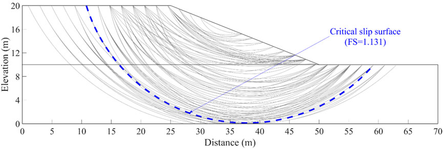
FIGURE 1. Slope geometry and schematics of RSSs for Example I.

TABLE 1

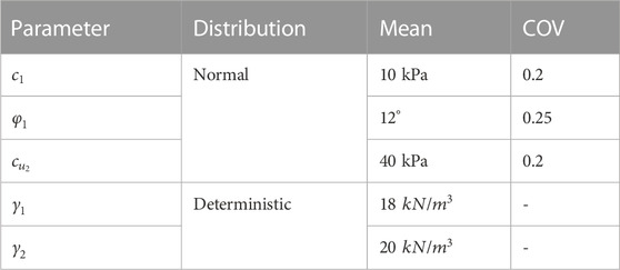
TABLE 1. Statistics of soil properties for Example I.

With the aforementioned mean parameters, the deterministic slope stability analysis is performed using the Bishop’s simplified method. A total of 4,250 PSSs are generated to cover the whole slope, and the FS of the CSS is 1.131, which is close to the value of 1.148 reported by Chowdhury and Xu (1995). Note that the FSs and the sliding volumes for the other PSSs are also calculated during the deterministic analysis, which can be conveniently used for the subsequent identification of RSSs. As mentioned before, a predefined range for the K value is a prerequisite for the adaptive K-means clustering method. From the previous study (Wang et al., 2020), an empirical range of [3, 200] is adopted herein. Then, the DUNN indices for different K values are obtained using the suggested procedure in Section 3 and Figure 2. The DUNN values are plotted against different K values. It can be seen from the figure that the K value has a significant effect on the DUUN index. As K is taken as 108, the DUNN index reaches the maximum, which means that clustering all PSSs into 108 sub-clusters is the best. Thereafter, the slip surface with the smallest FS in each of the 108 clusters is taken as the RSS of that cluster. Overall, 108 RSSs are finally identified and are also plotted in Figure 1. Note that the CSS signified by the dashed line in Figure 1 is also included in the final set of RSSs. To gain more insight into the effect of the clustering on PSSs, Figure 3 plots three typical clusters of the PSSs for the slope example. The figure shows that different clusters of slip surfaces exhibit different failure modes, and the slip surfaces in the same cluster present similar failure modes. For example, the slip surfaces of the 11th cluster plotted in Figure 3A are mainly shallow failure modes, whereas the slip surfaces in the 36th and 78th clusters tend to be much deeper.

FIGURE 2

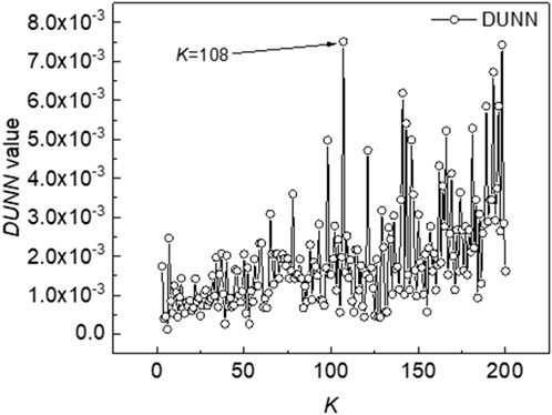
FIGURE 2. Variation of DUNN with K for Example I.

FIGURE 3

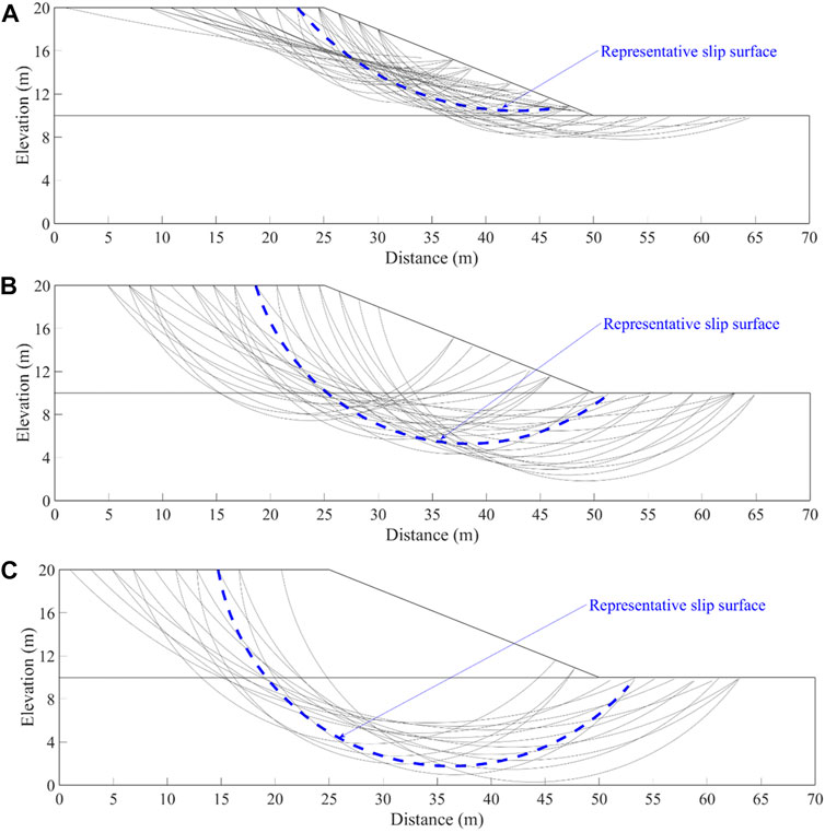
FIGURE 3. Typical clusters of PSSs for K=108 for the undrained cohesive slope of Example I. (A) The 11th cluster with 46 slip surfaces, (B) the 36th cluster with 30 slip surfaces, (C) the 78th cluster with 15 slip surfaces.

Response surfaces are then constructed based on the previously identified RSSs using $P_f$, followed by the MCS directly performed on the response surfaces to evaluate the $P_f$ of the slope. The $P_f$ is estimated as 0.398 and is very close to the value of 0.404 reported by Zhang et al. (2011), validating the accuracy of the method. The efficiency of the AKCBR can be approximately measured by a dimensionless nominal index $N_{ss}$ that indicates the total times of the FS evaluation of a single slip surface. Consider, for example, the deterministic slope stability analysis of the slope using 4,250 PSSs. The $N_{ss}$ is equal to 4,250 because 4,250 evaluations of the FS are required for the 4,250 PSSs. The computation cost for the reliability analysis of the AKCBR is mainly composed of 1) the time for identification of the RSSs and 2) the time for the calibration of the RSS-RSM. The first part can be equivalently evaluated using the actual physical time for the RSS identification divided by the time needed to calculate the FS of a single slip surface. For example, it takes about 0.001 s to calculate the FS of a single slip surface using a desktop computer with 16G RAM and an Intel(R) Core(TM) i9-9900x and 59 s to select the RSSs, so the $N_{ss}$ for the first part is approximately calculated as 59/0.001=59,000. In addition, the time of constructing the RSM and MCS with RSM is trivial and can be ignored. Therefore, the $N_{ss}$ for the AKCBR is about 63,250. In contrast, the time consumption of Method I (Zhang et al., 2011) is mainly for the evaluation of the reliability index of the 4,250 PSSs based on Eq. 1, and it takes about 80 s with the same computer. As such, the $N_{ss}$ for Method I is about 80,000, which is larger than that for the AKCBR.

5.2 Example II: an undrained cohesive slope considering 1-D ISV

This part applies the AKCBR for evaluating the reliability of an undrained cohesive slope to consider the ISV of the undrained shear strength $c_u$ in the vertical direction, which has also been studied in the literature (Wang et al., 2011; Li et al., 2013). The geometry of the slope is plotted in Figure 4, which has a slope height of 10 m and a slope angle of 26.6°. To enable a convenient and consistent comparison with previous studies, the mean of $c_u$ is 40 kPa, and the coefficient of variation is 0.25 (Wang et al., 2011; Li et al., 2013). The saturated unit weight ${\gamma }_{sat}$ of the soil is 20 kN/m³, which is considered as a deterministic value in this analysis. The undrained shear strength $c_u$, however, varies spatially in the vertical direction and has a mean ${\mu }_{c_u}$ and ${COV}_{c_u}$ of 40 kPa and 0.25, respectively. The ISV of $c_u$ is simulated by a stationary random field characterized by 40 random variables, which are the same as those used by Li et al. (2013) and described by the single exponential decaying correlation structure as

$R_{ij}=\exp \left(-\frac{z_i-z_j}{2\lambda }\right),(10)$

where $R_{ij}$ denotes the correlation between the soil properties at the depths $z_i$ and $z_j$, and $\lambda$ is the autocorrelation length. In theoretical engineering, $\lambda$ can be generally determined from a large quantity of measurement data, which is, however, often not available in practice. Therefore, different values of $\lambda$ varying from 0.5 to $+\infty$ are adopted to consider the effect of SOF on slope reliability assessment.

FIGURE 4

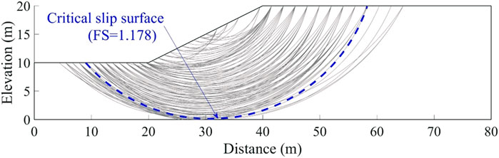
FIGURE 4. Geometry and RSSs of the undrained cohesive slope for Example II.

First, the deterministic slope stability analysis model was established using the aforementioned mean parameters, with 4,281 PSS covering the whole slope. The slope stability results are schematically shown in Figure 4, where the CSS passes through the bottom of the slope. The corresponding FS is 1.178, which is identical to the FS reported by Wang et al. (2011). Then, the 4,281 slip surfaces are divided into different clusters using the proposed adaptive K-means clustering method. The results show that when K is set as 154, the DUNN index reaches the maximum, signifying the optimal cluster number for the PSSs. Therefore, there are finally 154 RSSs identified for this slope example. All the RSSs are plotted in Figure 4, and the deterministic CSS is also included in the RSSs.

To illustrate the accuracy of the AKCBR, various parametric studies on the autocorrelation distances normalized by the slope height are conducted. As can be seen from Figure 5, the $P_f$ generally increases as the normalized autocorrelation distance increases. When $\frac{\lambda }{H}$ increases from 0.05 to 1 (or $\lambda$ increases from 0.5 to 10 m for H=10 m), the $P_f$ significantly increases from 1.3% to 28%, showing that the ISV has a significant influence on slope reliability. When $\frac{\lambda }{H}>0.5$, the $P_f$ becomes insensitive to the change of $\lambda$ as the spatial variety is nearly ignored. Figure 5 also includes the results of Wang et al. (2011) (based on MCS) and Li et al. (2013) (i.e., Method II), which agree well with the results from the current study and validate the accuracy of AKCBR. It is, however, worth noting that although the number of RSSs identified in this study is larger than that selected by Method II (Li et al., 2013), the proposed method still has eminent efficiency in reliability analysis. To illustrate this point, the dimensionless nominal index $N_{ss}$ is adopted again to compare the computation efficiency between the two methods. A desktop with 16G RAM and the Intel (R) Core(TM) i7-9700 k CPU requires about 0.001 s to evaluate the FS of a single slip surface. The $N_{ss}$ here for the AKCBR is thus approximately calculated as the summation of 1) the time for the deterministic analysis (i.e., 4,281), 2) the time for the identification of the RSSs (i.e., 73/0.001=73,000), and 3) the time for RSM calibration (i.e., (40×2+1)×154=12,474), which is about 89,755. In contrast, most of the computation cost for Method II is consumed by the calculation of the equivalent reliability index for all PSSs, which requires about 81 times the deterministic analysis, thus resulting in a $N_{ss}$ of about 346,761. It is obvious that the computation cost for Method II, even ignoring the subsequent reliability analysis, is higher than AKCBR with full analysis.

FIGURE 5

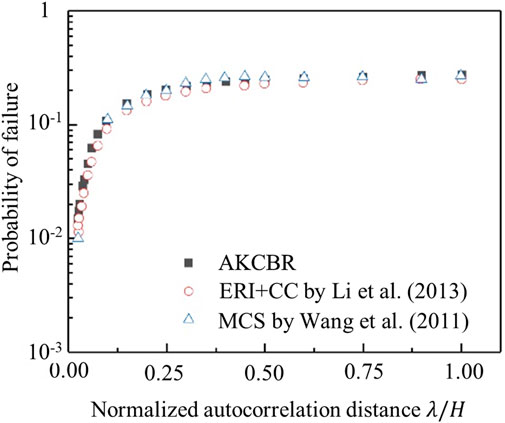
FIGURE 5. Results comparison considering spatial variability.

5.3 Example III: a cohesive-frictional slope considering 2-D ISV

This subsection takes a cohesive-frictional slope as an example to further illustrate the applicability and effectiveness of the AKCBR for reliability analysis considering 2-D ISV. The slope has been studied in the literature (Cho, 2010; Jiang et al., 2015; Liu et al., 2017; Liu et al., 2018), and the results from these available studies can be easily referred to. A similar slope study case was performed in Javankhoshdel et al. (2020). The cross-section of the slope is shown in Figure 6A, where the slope height and slope angle are 10 m and 45°, respectively. The total unit weight of the soil is 20 kN/m³. The cohesion $c$ and friction angle $\phi$ are considered spatially varied and characterized by two cross-correlated 2-D lognormal stationary random fields. The cross-correlation coefficient between $c$ and $\phi$ is −0.7. The mean values of $c$ and $\phi$ are, respectively, 10 kPa and 30°. The COV values of $c$ and $\phi$ are 0.3 and 0.2, respectively. The horizontal and vertical autocorrelation distances, ${\theta }_h$ and ${\theta }_v$, are 20 m and 2 m, respectively. All these parameters are consistent with those used in the literature (Cho, 2010; Jiang et al., 2015; Liu et al., 2017; Liu et al., 2018).

FIGURE 6

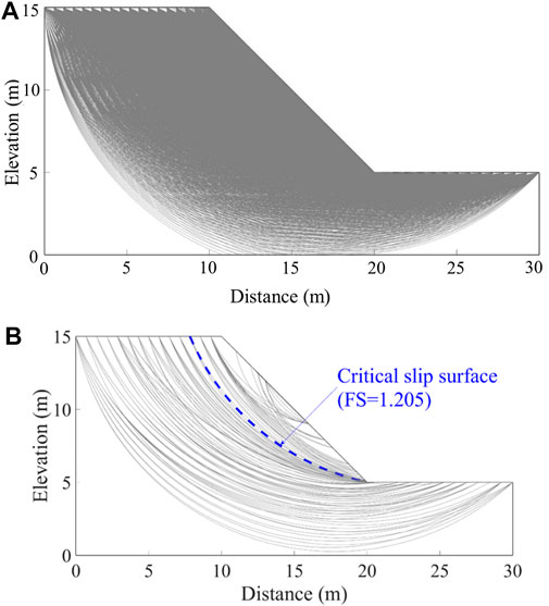
FIGURE 6. (A) Geometry of the cohesive-frictional slope for Example III with 7,436 PSSs, (B) RSSs identified for the cohesive-frictional slope for Example III.

Similar to the last slope example, the geometry of the slope is discretized into 1,210 random field elements with a side length of 0.5 m to consider the ISV of $c$ and $\phi$. The mid-point method is also adopted here to model the cross-correlated random fields of $c$ and $\phi$ with the squared exponential autocorrelation function. Then, slope stability analysis is performed to obtain the FS of the slope using Bishop’s simplified method. The FS is calculated as 1.205, and the associated CSS among 7,436 predefined PSSs is plotted in Figure 6A. The results are the same as those reported by Jiang et al. (2015), suggesting the accuracy of the slope stability analysis model.

Then, with the proposed adaptive K-means clustering method, the 7,436 slip surfaces are divided into different clusters. The results show that when K is set as 110, the DUNN index reaches the maximum, signifying the optimal cluster number for the PSSs. Therefore, there are finally 110 RSSs identified for this slope example. All the RSSs are plotted in Figure 6B, and the deterministic CSS is also one of the RSSs. With the RSSs, reliability analysis is performed using the proposed RSS-RSM in Section 4 to validate the effectiveness and efficiency of the adaptive K-means clustering approach for RSS identification. The $P_f$ based on adaptive K-means-based RSS-RSM is 4.4 × 10⁻³, and the $P_f$ values corresponding to Method III and MCS are 4.9 × 10⁻³ and 3.9 × 10⁻³ (Cho, 2010; Jiang et al., 2015). This similarity validates the accuracy of the AKCBR as well as the applicability for reliability analysis considering 2-D ISV. Note that Wang et al. (2020) previously analyzed the reliability of this example with the same approach but using a different number of RSSs. The reason is two-fold: 1) the number and locations of the PSSs here are different from those used by Wang et al. (2020); 2) the initial clustering centers are determined by an optimized method in MATLAB 2018b; they are randomly selected in MATLAB 2014a. Nevertheless, the reliability results from the two methods are very similar, indicating that the two methods successfully identified the RSSs.

To gain more insight into the AKCBR, the effect of the horizontal and vertical spatial variability on the reliability of the slope is further checked by the AKCBR in order to illustrate its effectiveness and efficiency against the variations of ${\theta }_h$ and ${\theta }_v$. The results are plotted in Figure 7. As a reference, the results from Liu et al. (2018) and Li et al. (2015) are also plotted in this figure. Note that, in the figure, only one parameter (i.e., ${\theta }_h$ or ${\theta }_v$) is changed for each case, while others are kept the same as previously defined. In general, the $P_f$ increases as the autocorrelation distances increase. The results obtained from this study show a good consistency with those from Liu et al. (2018) and Li et al. (2015). Such agreement suggests that the AKCBR is accurate and robust against the variation of ISV. Note that although Jiang et al. (2015) did not study the effect of ISV on the reliability of this slope example using their method, it is shown by a cohesive slope example application that their method is also robust against the variation of ISV. The AKCBR, therefore, is comparable with Method III in the accuracy of the reliability evaluation for a 2-D spatially varied slope.

FIGURE 7

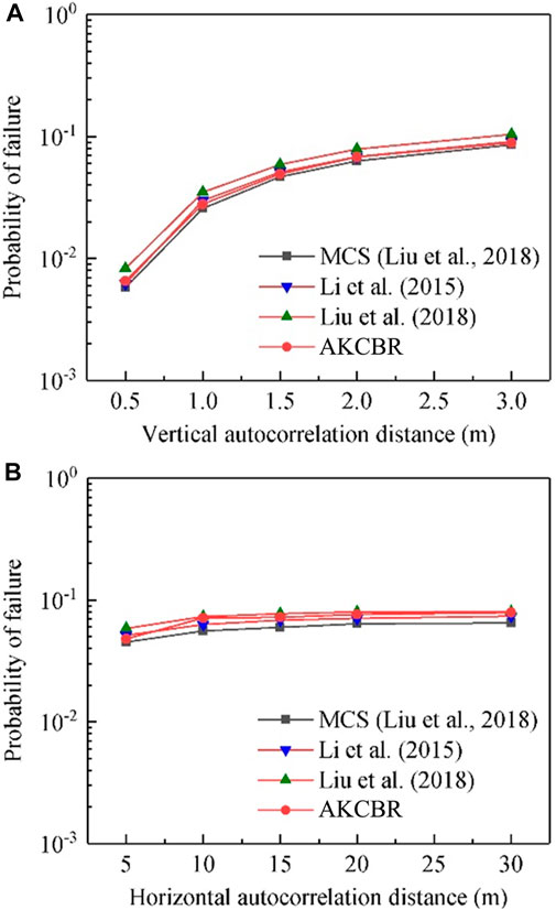
FIGURE 7. Effect of spatial variability on the failure probability of the slope in Example III. (A) Effect of ${\theta }_v$, (B) effect of ${\theta }_h$.

Jiang et al. (2015) also conducted a sensitivity study to investigate the effect of cross-correlation on the reliability of the slope. To keep a consistent comparison with Method III, the proposed method is also applied to this example to examine the influence of the cross-correlation coefficient. The results obtained by this study and from Method III are plotted in Figure 8A. It is seen from the figure that the $P_f$ obtained by this study increases from 0.44% to 6.8% as ${\rho }_{c\phi }$ varies from −0.7 to 0, suggesting a significant effect on $P_f$. Meanwhile, the results from Method III by Jiang et al. (2015) almost overlap those from the current study by the proposed adaptive K-means clustering-based RSS-RSM method, showing a good agreement between the two methods.

FIGURE 8

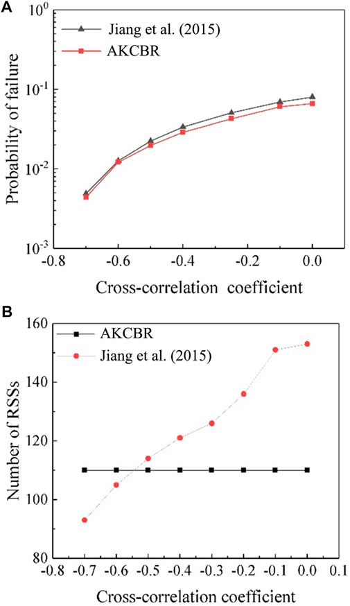
FIGURE 8. (A) Variation of $P_f$ with the cross-correlation coefficient, (B) variation of the number of RSSs with the cross-correlation coefficient.

The efficiency of the AKCBR can also be illustrated by the dimensionless index $N_{ss}$ used for the last two examples. The physical time for selecting the RSSs is about 69 s on a desktop computer with 16G RAM and Intel(R) Core(TM) i9-9900x, and 2,421 runs of the slope stability analysis model are required to calibrate the response surfaces of the 110 RSSs. This leads to the $N_{ss}$ of about $4\times {10}^5$ for the AKCBR. In contrast, it requires about an $N_{ss}$ of $7.4\times {10}^6$ to select the RSSs by Method III, where 1,000 LHS samples are generated to directly execute the slope stability analysis model with 7,436 PSSs. This comparison thus validates the efficiency of the AKCBR. In addition, note that the RSSs identified by Jiang et al. (2015) are sensitive to the variation of statistics of shear strengths (e.g., ISV and ${\rho }_{c\phi }$), which, however, is bypassed by the current study and will be further illustrated in the later discussion section. For example, Figure 8B compares the efficiency of the two methods in identifying the RSSs. It is observed that the AKCBR is independent of the ${\rho }_{c\phi }$, whereas the number of RSSs identified by Method III shows an increasing trend toward the increase of ${\rho }_{c\phi }$. This further indicates the high efficiency of the AKCBR.

5.4 Example IV: a layered cohesive slope considering 2-D ISV

This part analyzes the reliability of a layered cohesive slope using the AKCBR. The slope was also widely studied in the literature (Li D. Q. et al., 2016; Jiang et al., 2017; Wang et al., 2020) for reliability analysis. The geometry of the slope is schematically shown in Figure 9A, which has a slope height of 24 m and a slope angle of 36.9°; the slope is composed of two clayey soil layers. The statistics of the undrained shear strengths are the same as those used by Jiang et al. (2017). The mean of $c_u$ of layer 1 is 80 kPa, and the corresponding COV is 0.3. The mean of $c_u$ of layer 2 is 120 kPa, and the corresponding COV is 0.3. The parameter distributions of two layers of soil are both lognormal distributions. For the two layers the ${\theta }_h$ is 12 m, the ${\theta }_v$ is 1.2 m, and the unit weight is 19 kN/m³. Following Jiang et al. (2017), the slope geometry is discretized into a finite number (856) of random field elements, and the size of the element is kept consistent with Jiang et al. (2017) for convenient comparison. Deterministic slope stability analysis is then performed with 6,231 PSSs using Bishop’s simplified method. The FS is calculated as 1.447, and the corresponding CSS passes through the slope toe. These results are comparable with those reported by Jiang et al. (2017).

FIGURE 9

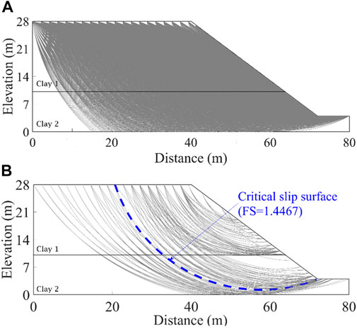
FIGURE 9. (A) Geometry of the layered cohesive slope for Example IV with 6,231 PSSs, (B) RSSs for the layered cohesive slope for Example IV.

With the AKCBR, 181 RSSs are identified, as schematically shown in Figure 9B, where the CSS is also included. Note that Wang et al. (2020) also previously analyzed the reliability of this example with the same approach but using a different number of RSSs. The reason is also two-fold and is the same as stated in the last example. The $P_f$ is subsequently estimated as 5.27×10⁻⁴ based on the RSS-RSM, which is comparable with the value of 5.13×10⁻⁴ by Method IV (Jiang et al., 2017) and those from other methods, as shown in Table 2. The consistency of the reliability results between different methods thus validates the accuracy of the AKCBR. Note that, however, the $N_{ss}$ of $2\times {10}^5$ for the AKCBR, estimated as that in the last example, is far less than that of $6\times {10}^6$ by Method IV. This consequently validates the computation efficiency of AKCBR.

TABLE 2

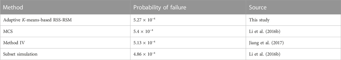
TABLE 2. Reliability analysis results obtained by different methods for Example IV.

6 Discussion

The aforementioned analysis shows that the AKCBR can enhance the efficiency of slope reliability analysis while maintaining accuracy and robustness. However, it is also noted that the number of RSSs identified by the AKCBR is generally larger than that identified by available methods. The reason might be that some trivial slip surfaces are included in the RSSs because of the empirical axiom for RSS identification, whereas the available methods can single out the key failure modes with more rigorous statistical fundamentals. For example, Methods II and IV identify the key failure modes of slopes with the contribution of each RSS to slope reliability. Therefore, to gain more insight into the differences between the AKCBR and other methods, this part further discusses the capability of the AKCBR in localizing the key failure modes of slopes from the perspectives of the locations of RSSs and the contributions of RSSs to slope reliability.

Figure 10 plots the locations of the RSSs by the proposed method and other methods. In the figure, the dotted lines represent the RSSs selected by this method, and the solid lines signify the RSSs by other methods. Generally, the RSSs selected by the AKCBR contain those selected by other methods. This indicates that the AKCBR is more conservative than other methods in determining the key failure modes but presents more variability. Again, the reason is mainly that the AKCBR relies only on the similarity of the shape and volume between different slip surfaces. Nevertheless, the AKCBR does not miss those key failure modes identified by other methods.

FIGURE 10

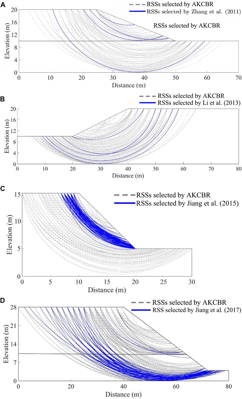
FIGURE 10. Comparison of RSSs selected by different methods. (A) Example I, (B) Example II, (C) Example III, (D) Example IV.

To quantify the contribution of each RSS to slope reliability, Figure 11 first plots the histograms of the numbers of failure samples for different RSSs selected by this method and other methods. Then, Figure 12 further quantifies the contribution of each RSS by a Pareto chart. Note that, in Figure 11, N_max and N_CSS indicate the maximum number of failure samples for an RSS and the number of failure samples of the CSS, respectively. It is observed from the histogram that, although there are more than 100 RSSs selected for each example, not all RSSs have a probability of failing. This shows that the contributions of different RSSs to slope reliability are different. For example, when ISV is not taken into consideration (Figure 11A), the slope probably may fail along only several (about four) of the RSSs with a large probability. This observation is also quantified by the proportion of the number of failures to the overall failures of an RSS, as shown in Figure 12A. It is seen from Figure 12A that the CSS and another RSS contribute almost 90% to the slope failure, with CSS taking up about 60%, and four failure modes can be found. It conforms with the traditional opinion of slope stability analysis that CSS is the most important failure mode of the slope. For other cases, it is found that as the degree of ISV increases (i.e., from Examples II to IV), more and more failure modes appear, and the CSS is no longer the most important one for slope failure. For example, the proportion of CSS contributing to the slope is the largest when 1-D ISV is considered in Example II (see Figures 11B, 12B), but it becomes not the most important RSS when 2-D ISV is considered in Example III (see Figures 11C,D, 12C,D). Therefore, it is insufficient to evaluate the reliability of a whole slope system using the CSS. These observations verify the available opinion that slope failure is a system problem considering many PSSs, and the slip surface with the minimum FS is not necessarily the slip surface with the maximum probability of failure. Overall, the aforementioned observations are consistent with those from other methods in the literature (Zhang et al., 2011; Li et al., 2013; Jiang et al., 2015; Jiang et al., 2017).

FIGURE 11

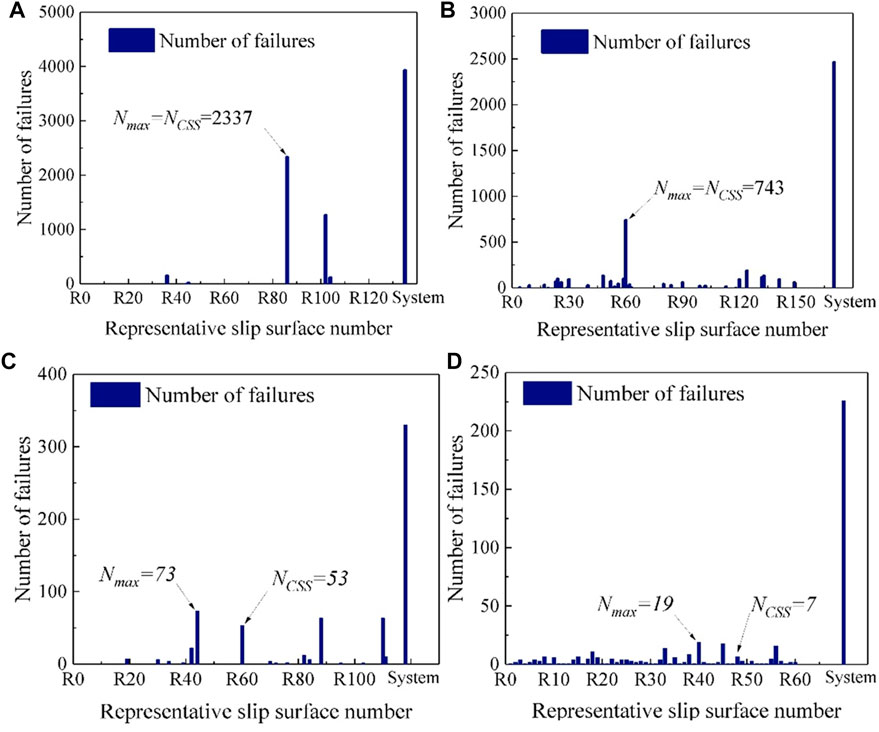
FIGURE 11. Histograms of the number of failure samples for different RSSs for different examples. (A) Example I, (B) Example II, (C) Example III, (D) Example IV.

FIGURE 12

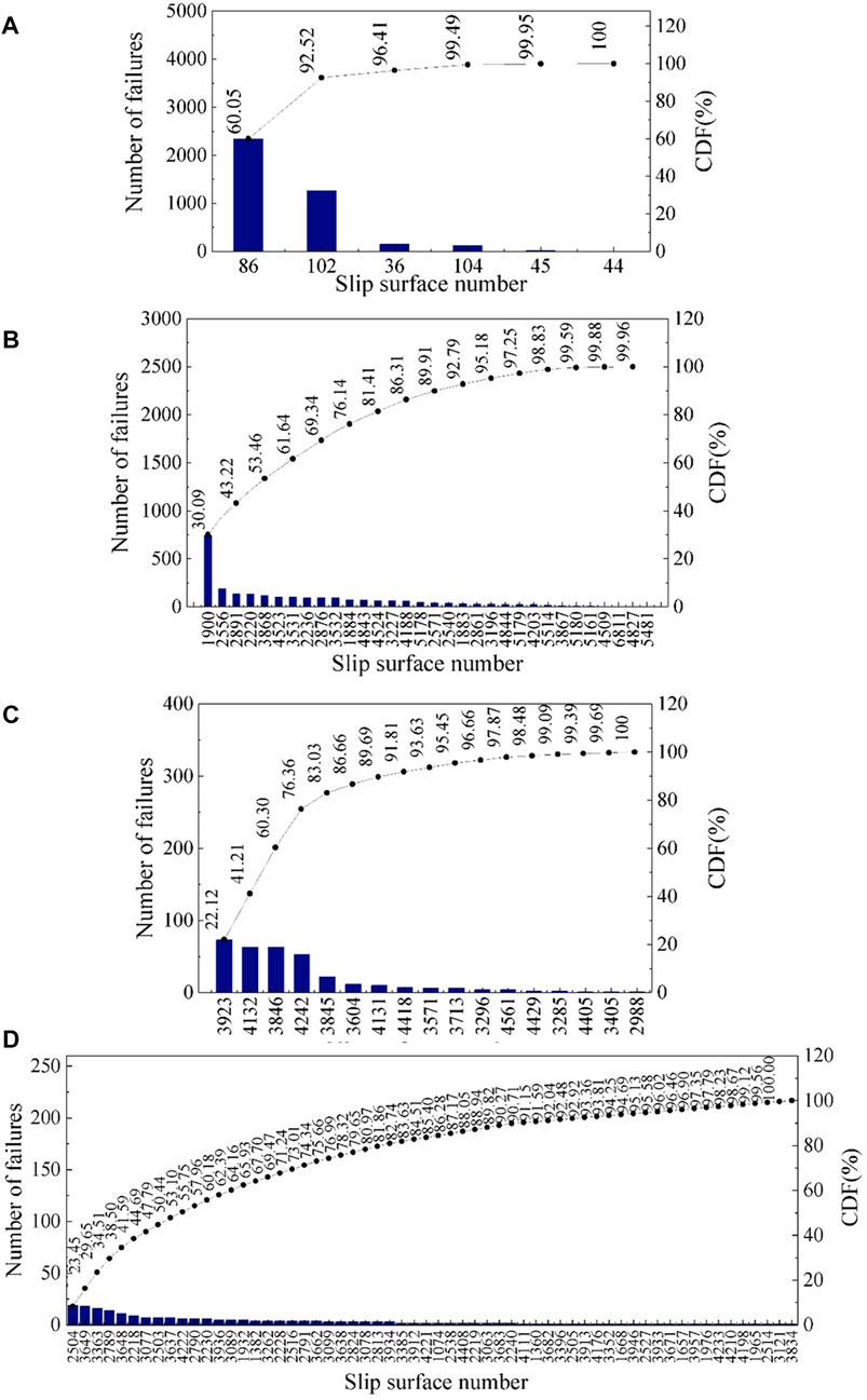
FIGURE 12. Pareto charts of the number of failure samples for different RSSs in different examples. (A) Example I, (B) Example II, (C) Example III, (D) Example IV.

Figure 13 presents the RSSs that contribute to the slope failure, where the solid lines represent RSSs selected by the proposed method, and the dashed lines represent the RSSs selected by other methods. Generally, the following observations can be obtained: (1) there are more failure modes identified by the proposed method than other methods; (2) the key failure modes identified by the proposed method and other methods are nearly at the same locations, being either the CSS or other RSSs; and (3) the potential failure areas identified by the proposed method and other methods almost overlap. These observations show that the proposed method can provide comparable information on slope failure modes with other methods.

FIGURE 13

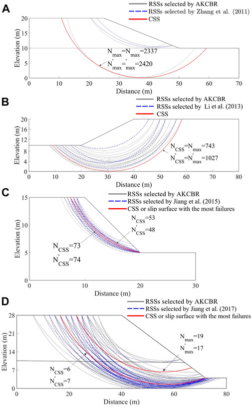
FIGURE 13. Comparison of RSSs that contribute to slope failure for different methods. (A) Example I, (B) Example II, (C) Example III, (D) Example IV.

7 Summary and conclusion

This paper applies a recently proposed method for identifying the RSSs of slopes, offering an efficient slope reliability analysis considering various situations. A comprehensive comparison between the AKCBR and other methods is presented from the perspective of computation accuracy and efficiency, as well as the capability for identifying the key failure modes of slopes. The fundamentals and procedures of the AKCBR and other methods are briefly reviewed. Four different slopes with different degrees of ISV are taken as illustrative examples to examine the effectiveness of AKCBR and elaborate the merits and limitations of the AKCBR against other methods. It is generally found that the number of RSSs identified by the AKCBR is much larger than that obtained by other methods because of the different axioms for different methods. However, the distributions of the RSSs obtained by different methods generally overlap, showing a good consistency between these methods in slope failure area detection. It is also observed that the AKCBR can identify almost the same key failure modes of slopes as other methods identify. For example, the CSS is identified by both the AKCBR and Method I as the critical reliability slip surface (CRSS) when ISV is ignored. When ISV is considered, the CSS is no longer the CRSS with the AKCBR and other methods. However, the AKCBR outweighs other methods in computation efficiency as the method requires only one execution of the deterministic slope model with an improved adaptive K-means clustering procedure. By contrast, other methods need either complex calculations of reliability indices for all PSSs or several random slope stability analyses. Overall, the AKCBR can provide comparable reliability results with other methods for different slope examples while offering a certain efficiency advantage.

Although the method is more efficient than the compared four methods, it is still necessary to clarify the limitations of the AKCBR and the merits of other methods. First, for the AKCBR, the number of RSSs is determined based on the number of clusters of PSSs, which is realized by an adaptive K-means clustering analysis on the PSSs. The clustering process, however, depends only on the number and volumes of PSSs, regardless of the change in soil statistics. This, therefore, allows the method to be efficiently and conveniently applied to reliability analysis involving many parametric studies, especially for situations where the ISV is not clearly known by engineers. Then, other methods, such as Method I and II, although a complex calculation on reliability indices of all PSSs is required, are statistically more rigorous than the AKCBR. Similar to Method IV, the AKCBR is also considered an empirical or semi-empirical method for RSS identification. Finally, it is worth noting that the limit equilibrium method with circular failure mechanism assumption (i.e., Bishop’s simplified method) is adopted in the current study, so the application of the AKCBR to slope reliability analysis with non-circular slip surfaces remains open and requires further study.

Data availability statement

The raw data supporting the conclusion of this article will be made available by the authors, without undue reservation.

Author contributions

W-QZ carried out the data analysis and wrote the content, S-HZ designed the study and wrote the content, Y-HL carried out the data analysis, and JL carried out the data analysis and wrote the content. All authors have read and approved the final manuscript. All authors listed have made a substantial, direct, and intellectual contribution to the work and approved it for publication.

Acknowledgments

The authors would like to thank Lei-Lei Liu from the Central South University for shaping the idea of the presented work and some useful suggestions.

Conflict of interest

The authors declare that the research was conducted in the absence of any commercial or financial relationships that could be construed as a potential conflict of interest.

Publisher’s note

All claims expressed in this article are solely those of the authors and do not necessarily represent those of their affiliated organizations, or those of the publisher, the editors, and the reviewers. Any product that may be evaluated in this article, or claim that may be made by its manufacturer, is not guaranteed or endorsed by the publisher.

Supplementary material

The Supplementary Material for this article can be found online at: https://www.frontiersin.org/articles/10.3389/feart.2023.1100104/full#supplementary-material

References

Ang, A. H. S., and Tang, W. H. (2007). Probability concepts in engineering: Emphasis on applications to civil and enviromental engineering. Chichester, UK: Wiley.

Google Scholar

Benesty, J., Chen, J., Huang, Y., and Cohen, I., 2009, Pearson correlation coefficient, Berlin, Heidelberg, Springer Berlin Heidelberg, Noise Reduction in Speech Processing, 37–40.

Google Scholar

Bhattacharya, G., Jana, D., Ojha, S., and Chakraborty, S. (2003), Direct search Minim. Reliab. index earth slopes Comput. Geotechnics 30 (6), 455–462.

CrossRef Full Text

Cho, S. E. (2010). Probabilistic assessment of slope stability that considers the spatial variability of soil properties. J. geotechnical geoenvironmental Eng. 136 (7), 975–984. doi:10.1061/(asce)gt.1943-5606.0000309

CrossRef Full Text | Google Scholar

Chowdhury, R. N., and Xu, D. W. (1995). Geotechnical system reliability of slopes. Reliab. Eng. Syst. Saf. 47 (3), 141–151. doi:10.1016/0951-8320(94)00063-t

CrossRef Full Text | Google Scholar

Chu, X., Li, L., and Wang, Y. (2015). Slope reliability analysis using length-based representative slip surfaces. Arabian J. Geosciences 8 (11), 9065–9078. doi:10.1007/s12517-015-1905-5

CrossRef Full Text | Google Scholar

Dunn, J. C. (1974). Well-Separated Clusters and Optimal Fuzzy Partitions. Journal of Cybernetics 4 (1), 95–104.

CrossRef Full Text | Google Scholar

Huang, S.-Y., Zhang, S.-H., and Liu, L.-L. (2022). A new active learning Kriging metamodel for structural system reliability analysis with multiple failure modes. Reliability Engineering & System Safety 228.

CrossRef Full Text | Google Scholar

Jamshidi Chenari, R., and Alaie, R. (2015). Effects of anisotropy in correlation structure on the stability of an undrained clay slope. Georisk Assess. Manag. Risk Eng. Syst. Geohazards 9 (2), 109–123. doi:10.1080/17499518.2015.1037844

CrossRef Full Text | Google Scholar

Javankhoshdel, S., Cami, B., Chenari, R. J., and Dastpak, P. (2020). Probabilistic analysis of slopes with linearly increasing undrained shear strength using RLEM approach. Transp. Infrastruct. Geotechnol. 8 (1), 114–141. doi:10.1007/s40515-020-00118-7

CrossRef Full Text | Google Scholar

Ji, J., and Low, B. K. (2012). Stratified response surfaces for system probabilistic evaluation of slopes. J. Geotechnical Geoenvironmental Eng. 138 (11), 1398–1406. doi:10.1061/(asce)gt.1943-5606.0000711

CrossRef Full Text | Google Scholar

Jiang, Q., Liu, J., Zheng, H., Wang, B., Guo, Z.-Z., Chen, T., et al. (2022a). Bayesian estimation of rock mechanical parameter and stability analysis for a large underground cavern. Int. J. Geomechanics 22 (8), 04022129. doi:10.1061/(asce)gm.1943-5622.0002452

CrossRef Full Text | Google Scholar

Jiang, S.-H., Huang, J., Qi, X.-H., and Zhou, C.-B. (2020). Efficient probabilistic back analysis of spatially varying soil parameters for slope reliability assessment. Eng. Geol., 271.

CrossRef Full Text | Google Scholar

Jiang, S.-H., Liu, X., Huang, J., and Zhou, C.-B. (2022b). Efficient reliability-based design of slope angles in spatially variable soils with field data. Int. J. Numer. Anal. Methods Geomechanics 46 (13), 2461–2490. doi:10.1002/nag.3414

CrossRef Full Text | Google Scholar

Jiang, S.-H., Papaioannou, I., and Straub, D. (2018). Bayesian updating of slope reliability in spatially variable soils with in-situ measurements. Eng. Geol. 239, 310–320. doi:10.1016/j.enggeo.2018.03.021

CrossRef Full Text | Google Scholar

Jiang, S. H., Huang, J., Yao, C., and Yang, J. (2017). Quantitative risk assessment of slope failure in 2-D spatially variable soils by limit equilibrium method. Appl. Math. Model. 47, 710–725. doi:10.1016/j.apm.2017.03.048

CrossRef Full Text | Google Scholar

Jiang, S. H., Li, D. Q., Cao, Z. J., Zhou, C. B., and Phoon, K. K. (2015). Efficient system reliability analysis of slope stability in spatially variable soils using Monte Carlo simulation. J. Geotechnical Geoenvironmental Eng. 141 (2), 04014096. doi:10.1061/(asce)gt.1943-5606.0001227

CrossRef Full Text | Google Scholar

Li, D.-Q., Jiang, S.-H., Cao, Z.-J., Zhou, W., Zhou, C.-B., and Zhang, L.-M. (2015). A multiple response-surface method for slope reliability analysis considering spatial variability of soil properties. Eng. Geol. 187, 60–72. doi:10.1016/j.enggeo.2014.12.003

CrossRef Full Text | Google Scholar

Li, D.-Q., Zheng, D., Cao, Z.-J., Tang, X.-S., and Phoon, K.-K. (2016a). Response surface methods for slope reliability analysis: Review and comparison. Eng. Geol. 203, 3–14. doi:10.1016/j.enggeo.2015.09.003

CrossRef Full Text | Google Scholar

Li, D. Q., Qi, X. H., Cao, Z., Tang, X. S., Phoon, K. K., and Zhou, C. B. (2016b). Evaluating slope stability uncertainty using coupled Markov chain. Comput. Geotechnics 73, 72–82. doi:10.1016/j.compgeo.2015.11.021

CrossRef Full Text | Google Scholar

Li, L., and Chu, X. (2016). Risk assessment of slope failure by representative slip surfaces and response surface function. KSCE J. Civ. Eng. 20 (5), 1783–1792. doi:10.1007/s12205-015-2243-6

CrossRef Full Text | Google Scholar

Li, L., Wang, Y., Cao, Z., and Chu, X. (2013). Risk de-aggregation and system reliability analysis of slope stability using representative slip surfaces. Comput. Geotechnics 53, 95–105. doi:10.1016/j.compgeo.2013.05.004

CrossRef Full Text | Google Scholar

Li, L., Wang, Y., and Cao, Z. (2014). Probabilistic slope stability analysis by risk aggregation. Eng. Geol. 176, 57–65. doi:10.1016/j.enggeo.2014.04.010

CrossRef Full Text | Google Scholar

Liu, J., Jiang, Q., Chen, T., Yan, S., Ying, J., Xiong, X., et al. (2022a). Bayesian estimation for probability distribution of rock’s elastic modulus based on compression wave velocity and deformation warning for large underground cavern. Rock Mech. Rock Eng. 55, 3749–3767. doi:10.1007/s00603-022-02801-2

CrossRef Full Text | Google Scholar

Liu, L.-L., and Cheng, Y.-M. (2016). Efficient system reliability analysis of soil slopes using multivariate adaptive regression splines-based Monte Carlo simulation. Comput. Geotechnics 79, 41–54. doi:10.1016/j.compgeo.2016.05.001

CrossRef Full Text | Google Scholar

Liu, L.-L., Cheng, Y.-M., and Zhang, S.-H. (2017). Conditional random field reliability analysis of a cohesion-frictional slope. Comput. Geotechnics 82, 173–186. doi:10.1016/j.compgeo.2016.10.014

CrossRef Full Text | Google Scholar

Liu, L.-L., Deng, Z.-P., Zhang, S.-h., and Cheng, Y.-M. (2018). Simplified framework for system reliability analysis of slopes in spatially variable soils. Eng. Geol. 239, 330–343. doi:10.1016/j.enggeo.2018.04.009

CrossRef Full Text | Google Scholar

Liu, L.-L., and Wang, Y. (2022). Quantification of stratigraphic boundary uncertainty from limited boreholes and its effect on slope stability analysis. Eng. Geol. 306, 106770. doi:10.1016/j.enggeo.2022.106770

CrossRef Full Text | Google Scholar

Liu, L.-L., Yang, C., and Wang, X.-M. (2021). Landslide susceptibility assessment using feature selection-based machine learning models. Geomechanics Eng. 25 (1), 1–16.

Google Scholar

Liu, L.-L., Zhang, P., Zhang, S.-H., Li, J.-Z., Huang, L., Cheng, Y.-M., et al. (2022b). Efficient evaluation of run-out distance of slope failure under excavation. Eng. Geol. 306, 106751. doi:10.1016/j.enggeo.2022.106751

CrossRef Full Text | Google Scholar

Low, B. K., and Tang, W. H. (2007). Efficient spreadsheet algorithm for first-order reliability method. J. Eng. Mech. 133 (12), 1378–1387. doi:10.1061/(asce)0733-9399(2007)133:12(1378)

CrossRef Full Text | Google Scholar

Ma, J. Z., Zhang, J., Huang, H. W., Zhang, L. L., and Huang, J. S. (2017). Identification of representative slip surfaces for reliability analysis of soil slopes based on shear strength reduction. Comput. Geotechnics 85, 199–206. doi:10.1016/j.compgeo.2016.12.033

CrossRef Full Text | Google Scholar

Mafi, R., Javankhoshdel, S., Cami, B., Jamshidi Chenari, R., and Gandomi, A. H. (2020). Surface altering optimisation in slope stability analysis with non-circular failure for random limit equilibrium method. Georisk Assess. Manag. Risk Eng. Syst. Geohazards 15 (4), 260–286. doi:10.1080/17499518.2020.1771739

CrossRef Full Text | Google Scholar

Phoon, K. K., and Ching, J. (2014). Risk and reliability in geotechnical engineering. Boca Raton: CRC Press.

Google Scholar

Phoon, K. K., and Retief, J. V. (2016). Reliability of geotechnical structures in ISO2394. London: Taylor & Francis.

Google Scholar

Wang, B., Liu, L., Li, Y., and Jiang, Q. (2020). Reliability analysis of slopes considering spatial variability of soil properties based on efficiently identified representative slip surfaces. J. Rock Mech. Geotechnical Eng. 12, 642–655. doi:10.1016/j.jrmge.2019.12.003

CrossRef Full Text | Google Scholar

Wang, Y., Cao, Z., and Au, S.-K. (2011). Practical reliability analysis of slope stability by advanced Monte Carlo simulations in a spreadsheet. Can. Geotechnical J. 48 (1), 162–172. doi:10.1139/t10-044

CrossRef Full Text | Google Scholar

Zhang, J., Zhang, L. M., and Tang, W. H. (2011). New methods for system reliability analysis of soil slopes. Can. Geotechnical J. 48 (7), 1138–1148. doi:10.1139/t11-009

CrossRef Full Text | Google Scholar

Zheng, D., Li, D.-Q., Cao, Z.-J., Tang, X.-S., and Phoon, K.-K. (2016). An analytical method for quantifying the correlation among slope failure modes in spatially variable soils. Bull. Eng. Geol. Environ. 76 (4), 1343–1352. doi:10.1007/s10064-016-0923-1

CrossRef Full Text | Google Scholar