 Lorenz M. Fischer
 Christian Sommer
 Kathryn E. Fitzsimmons
- 1Department of Geosciences, University of Tuebingen, Tuebingen, Germany
- 2Department of Geosciences, Institute of Geography, University of Tuebingen, Tuebingen, Germany
- 3Heidelberg Academy of Sciences and Humanities, ROCEEH—The Role of Culture in Early Expansions of Humans, Tuebingen, Germany
Future climate projections indicate an expansion of the world’s drylands, and with that a commensurate increase in the mobilization of unconsolidated desert sediments such as sand and dust. It is therefore increasingly important to investigate the large-scale formation of dryland landscapes such as dunefields in order to better understand the processes responsible for their genesis, evolution, and thresholds for mobilization. Assessing dunefield morphologic variability, including analysis of the morphologic relationship between aeolian bedforms and other landforms such as fluvial channels and bedrock uplands, underpins such investigations. So far, however, meaningful investigations of erg-scale geomorphic patterns have been limited. This is in part due to the technological limitations of geographic information system (GIS) tools, particularly in the case of open-source datasets and software, which has effectively hindered investigations by colleagues in drylands of the global south where many of the world’s dunefields are located. Recent years have overseen the increasing availability of open-source remote sensing datasets, as well as the development of freely available software which can undertake geographic object-based image analysis (GEOBIA). These new tools facilitate cartography and statistical analysis of dunefields at large scales. In this study we make use of open-source GIS to characterise a morphologically diverse linear dunefield southwest of Kati Thanda (Lake Eyre) in central Australia. We focus on three parameters; dune orientation, spacing and Y-junctions using semi-automated GEOBIA, and investigate these in the context of local fluvial channels, depressions (pans) and uplands. Our results suggest a possible correlation between dune orientation, wind regime and the role of uplands as deflective barriers to longitudinal dune migration; dune spacing and sediment supply, likely relating to the location of both ephemeral and abandoned fluvial channels; and Y-junction frequency with underlying topography. Our study provides a framework for understanding process-based interactions between dunes and other landforms, as well as the first completely open-source approach which can be applied to linear dunefields worldwide.
1 Introduction
The world’s drylands, which currently comprise almost half of the land surface (Koutroulis, 2019) and host one-quarter of Earth’s human population (Reynolds et al., 2007), may expand in response to anthropogenic climate change (Huang et al., 2016; 2017; Parteli, 2022). The mobilization of unconsolidated desert sediments, such as sand and dust, represents an increasing hazard as drylands areas expand (Thomas et al., 2005; Gholami et al., 2021; Parteli, 2022). Further land areas susceptible to desertification relating to land use and soil loss comprise an additional sediment hazard (Mirzabaev et al., 2022). Dunefields, which represent one-fifth of the world’s dryland area (Bailey and Thomas, 2014), are a major source of aeolian sand which can be reactivated (Parteli, 2022). However, it is difficult to meaningfully assess future risk of sediment mobilization due the poor understanding of the multiple processes responsible for the genesis, evolution, and erosion thresholds in dunefields. In part, our poor understanding is due to the limited number of studies on dunefield-scale morphologic variability and the geomorphic relationship between dunes and other landforms within bordering dunefields, such as fluvial channels, pans and playas, and bedrock uplands (Krapf et al., 2003; Svendsen et al., 2003).
Although a range of dune morphologies exist, linear (or longitudinal) dunes are some of the most common (Telfer and Hesse, 2013; Radebaugh et al., 2015). Vegetated linear dunes (VLD) form broadly parallel to the resultant vector of the sand-shifting winds at the time of their formation (Tsoar, 1989; Tsoar, 2001; Pye and Tsoar, 2008), and often result from alternating wind directions which transport sand onto and along both dune flanks (Bristow et al., 2000; Tsoar, 2001; Bristow et al., 2010; Courrech du Pont et al., 2014). The lack of bedform lateral migration ensures that the longitudinal morphology of linear dunes may be preserved over tens, and sometimes hundreds, of kilometers downwind (Jennings, 1968; Mabbutt, 1968; Twidale, 1968; Tsoar, 2005). Although the process of linear dune elongation has been the subject of investigations at the level of individual bedforms (Hugenholtz et al., 2012; Rozier et al., 2019; Baddock, et al., 2021), the relationship between linear dunes and other landforms within a dunefield is as yet poorly defined (Hollands et al., 2006; Al-Masrahy and Mountney, 2015; Liu and Coulthard, 2015). Whilst it is clear that dune morphology can be influenced by physical barriers, water bodies and vegetation cover (Tsoar, 1978; Fryberger and Dean, 1979; Hesse and Simpson, 2006; Fitzsimmons, 2007; Roskin et al., 2014; Fitzsimmons et al., 2020), these interactions have so far been inadequately characterized and quantified.
The mapping of linear dunefields using remote sensing and geographic information systems (GIS) is one of the best ways to characterize dune parameters over large spatial scales, and to investigate the formation of dunes and their interactions with other landforms (Siegal et al., 2013). Until recently, however, these sorts of studies have been hampered by technological limitations and by a lack of affordable GIS options (Baddock et al., 2021; Zheng et al., 2022). While remote sensing has long been used to map dunefields (Tsoar, 1978; Breed and Grow, 1979), earlier studies involved time-consuming manual digitization of dune crests (Wasson et al., 1988; Bullard et al., 1995; Fitzsimmons, 2007; Ewing and Kocurek, 2010; Roskin et al., 2011; Telfer, et al., 2017; Gavrilov et al., 2018) which were both subjective and poorly suited to large-scale cartography. More recently, machine learning has been applied to generate dune maps (Fitzsimmons et al., 2020; Shumack et al., 2020; Rubanenko et al., 2021) but still requires substantial and costly computational resources (Yuan et al., 2020) which are not readily available, for example, in the global south where the world’s dunefields are overwhelmingly located.
In this study, we propose a low-cost, entirely open-source approach to mapping both types of vegetated and non-vegetated linear dunefields. We use this workflow to assess and quantify dune morphological variability, and to investigate the relationships between dune morphology and other landforms. By introducing an easily implemented, semi-automated cartographic method, we hope to remove some of the barriers to investigating dryland environments for colleagues with more limited resources, and who are likely to be directly impacted by the increasing risks associated with dryland sediment mobilization.
Our study focusses on a linear dunefield with a high degree of morphologic variability on the southwestern margins of Kati Thanda (Lake Eyre) in Central Australia. In this context we define morphological variability in terms of a range of dune spacing, orientation, frequency of Y-junctions and likely interactions with other landforms. Y-shaped merging dunes formed in a downwind direction are hereby understood as Y-junctions (Fitzsimmons, 2007). We also refer to Y-junctions as “dune junctions” and will use these terms interchangeably. The rationale was to undertake a proof of concept for our open-source GIS approach using a well-defined, relatively small area, after which the method can be scaled up to larger dunefields. We undertake semi-automated dunefield mapping. By deriving dune morphological data across the mapped region, we aim to characterize and quantify dune orientation, spacing and Y-junction frequency. Finally, we will examine the relationship between these parameters and possible driving factors such as climate, regional topography and the distribution of other landforms.
2 Materials and methods
2.1 Kati Thanda (Lake Eyre) mapping area
More than one-third of the Australian mainland is occupied by desert linear dunefields, which are distributed in an anticlockwise whorl about the centre of the continent (Jennings, 1968; Hesse, 2010). Linear dunefields in central Australia experience the greatest variability in orientation compared with those on the arid periphery (Hesse, 2010). Other landforms including playa lakes, uplands, stony desert and floodplain substrates, and active, ephemeral and abandoned fluvial channels also occur in the desert (Fitzsimmons, 2007).
We focus on a small (c. 8450 km2) dunefield located on the southwest margins of Kati Thanda (Lake Eyre) in central Australia (in the north of the state of South Australia) (Figure 1). Our research area was selected because of its high degree of morphologic variability within a relatively small area, as well as the presence of bedrock uplands, chains of playas and fluvial channels. This setting facilitates an investigation of the interaction between dune morphologic parameters and other landforms.
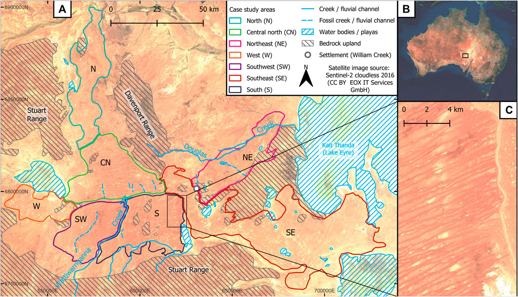
FIGURE 1. Map showing the location of the study areas, drainage features, water bodies and bedrock upland parts (A), the location of the study site within Australia (B) and an enlarged snippet showing dunes and a chain of playas (C).
Kati Thanda lies within the most arid region of Australia. It experiences 150 mm of rainfall on average per year, with substantial inter-annual variability (Simon-Coinçon et al., 1996) and no clear seasonal dominance of precipitation (Magee et al., 2004). Kati Thanda (Lake Eyre) is the terminal playa lake of an endorheic basin which occupies approximately 15% of the Australian mainland (May et al., 2022). Kati Thanda (Lake Eyre) overlies the Mesozoic Eromanga basin (Krapf et al., 2022); arid conditions have persisted in the basin since the Pliocene (Fujioka et al., 2005). The Kati Thanda dunefield which forms our focus is bordered to the north by the Davenport Range, which rises 140 m above the dunes and comprises Neoproterozoic sediments and intrusive mafic rocks (Cowley et al., 2020). The Stuart Range lies to the west and south of the dunefield and consists of deformed lower Cretaceous Eromanga Basin sediments (Drexel et al., 1995). Kati Thanda, with its generally dry lake bed of clays and salt crust, lies to the east and northeast of the dunefield. Clayey through sandy Eromanga Basin rocks occasionally crop out along the playa shoreline (Drexel et al., 1995; Cowley et al., 2020) and are in many places cemented by silcrete and ferricrete (Krapf et al., 2018; Wakelin-King, 2022). We assume the linear dunefields to have formed from the early Pleistocene onward (Fujioka et al., 2009), periodically activating during phases of intensified aridity and increased sediment supply throughout the Pleistocene and into the Holocene, as has been found to be the case elsewhere within the Lake Eyre Basin (Hollands et al., 2006; Fitzsimmons, 2007; Fitzsimmons et al., 2013).
The dunefield itself is sparsely vegetated and the dunes appear to be largely inactive (Wopfner and Twidale, 1988; Hesse, 2010) or in a state of partial activity, with bedforms retaining a stable morphology (Hesse and Simpson, 2006). Overall, the linear dunes of the study area shift from a predominantly WSW-ENE orientation in the southwest to a more N-S direction in the far north and east (Figure 1) and lie on the southeastern edge of the anticlockwise linear dune whorl observed across the Australian continent by previous workers (Wasson et al., 1988). Linear dunes are postulated to broadly result from aeolian transport parallel to the resultant wind vector at the time of formation (Tsoar et al., 2004; Pye and Tsoar, 2008).
The elevation of the dunefield ranges from 110 m asl on its western margins to −10 m at the shoreline of Kati Thanda, along a 120 km transect. We observe a range of non-aeolian landforms within the study dunefield. These include several small playas, including chains of depressions which align north-south and parallel Kati Thanda, and may represent abandoned fluvial depressions or lake floor (Wakelin-King, 2022). Several ephemeral creeks drain eastward into the lake (Armon et al., 2020; May and Worthy, 2022), and we observe a number of local drainage systems are associated with individual small playas (Hesse, 2010). Several fossil and active mound springs associated with discharge from the underlying Great Artesian Basin (Boucaut et al., 1986; Fitzsimmons, 2005) occur within the dunefield.
We selected three smaller case study areas within the dunefield in order to maximize the efficiency of data acquisition (Figure 1). These are described as the centre north (CN), northeast (NE) and southwest (SW) case study areas (Sections 2.1.1–2.1.3, respectively). Other areas (north, west, center-south and southeast), which were not investigated in as much detail but discussed in part below, are delineated in Figure 1.
2.1.1 Centre north (CN) case study area
The CN case study area is situated in the central part of the dunefield and is defined by the Stuart Range to the west, Davenport Range to the east and the Wattiwarriganna Creek to the south. The northern boundary is arbitrary and was defined by eye as a zone of rapid change in dune orientation from WSW-ENE to SW-NE and an upland rise associated with more widely spaced dunes to the north (Figure 1). Upon initial inspection, the CN area is characterized by an overall change in dune morphology from west to east, which may be associated with a north-south bedrock ridge (Cowley et al., 2020). This change of dune morphology, as well as the occurrence of topographic features made the examination of this case study area for us worth studying. The CN area covers 1,219 km2.
2.1.2 Northeastern (NE) case study area
The NE case study area is a northeast-trending lobe of linear dunes extending from the main dunefield towards the shoreline of Kati Thanda and has an area of 974 km2. Bedrock crops out to the north and south of the NE dune lobe. The Douglas Creek flows parallel to the dunefield margins towards the northern boundary of the area. The eastern and southeastern margins are bounded by desert pavement (gibber) and silcretes (Alley, 1998; Krapf et al., 2018). The southwestern margins of the area are marked by the settlement of William Creek and two playas. Several chains of playas run NW-SE through this area and may represent fossil drainage depressions (Krapf et al., 2018). The wider dune distances, as well as the occurring of an active and fossil creek determined the investigation of this case study area.
2.1.3 Southwestern (SW) case study area
The SW case study area adjoins the southern margins of the CN area. This is the smallest case study area with 833 km2. The bedrock uplands of the Stuart Range bound the dunefield to the west and south here, and its eastern margins are demarcated by the Wattiwarriganna Creek. It should also be noted that the case study area hosts two NW-SE oriented chains of playas, which represent topographic depressions in the underlying relief and may influence dune morphology. The dunes appear to be more closely spaced than elsewhere in the dunefield. For those reasons, the area was chosen for examination.
2.2 Remote sensing: datasets and pre-processing
Our study makes use of several data processing methods (for a detailed overview, refer to Supplementary Material). We used satellite remote sensing data to produce terrain information for our assessment of topographic features. We then extracted dunefield morphologic data using semi-automated GIS in the form of Geographic Object-Based Image Analysis (GEOBIA; Section 2.3).
Since our ultimate aim was to use this workflow (Figure 2) to investigate interactions between linear dunes and other landscape types, we first characterized the regional terrain using remote sensing-derived digital elevation models (DEMs). The challenge for our chosen study area is its relatively subdued height variation (c. 120 vertical meters; see Section 2.1); a particularly high-resolution DEM was therefore necessary to detect the subtle changes in elevation. Following visual inspection and literature review of seven open-source DEMs (Uuemaa et al., 2020), we selected the AW3D30 Digital Surface Model (DSM), using the Japan Aerospace Exploration Agency (JAXA) dataset and remote-sensing data derived from the Panchromatic Remote-sensing Instrument for Stereo Mapping (PRISM) aboard the Advanced Land Observing Satellite (ALOS). AW3D30 is a freely available downscaled version of a higher resolution commercial photogrammetric DSM and exhibits high robustness and vertical accuracy compared to its competitors (Courty et al., 2019; Uuemaa et al., 2020), Furthermore, its permissive license fits in our general framework using open software and data. These merits outweigh the advantages of genuine DTMs (with vegetation, human made structures, etc.), that play little role for our chosen region since there is minimal human impact and neglectable vegetation cover on the dunefield. We worked with six AW3D30 tiles (each one degree of latitude and longitude in area) to produce a DSM with pixel resolution of c. 27.5 m (Longley, 2005) (see Supplementary Figure S15).
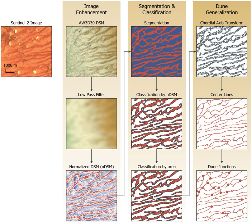
FIGURE 2. Graphical overview of the OBIA workflow for dune classification and derivation of parameters.
Data pre-processing was undertaken using the free, open-source software SAGA GIS Version 7.8.2 (System for Automated Geoscientific Analysis; Conrad et al., 2015). SAGA GIS is compatible with the freeware QGIS (QGIS-Development-Team, 2022) which was used to classify dune morphological categories and to undertake the mapping. We merged the six data tiles into a single grid using the SAGA GIS mosaic tool, resampling using the nearest neighbor option. Following alignment of the input data, we projected the dataset into the Universal Transverse Mercator (UTM) 53-south grid (UTM zone 53 J), using EPSG code 32753 and the UTM projection tool in SAGA GIS, again using Nearest Neighbour resampling. We improved processing efficiency by reducing data frame size, clipping the input grid using a polygon shapefile containing the study area outline in QGIS.
2.3 Dunefield mapping using geographic object-based image analysis (GEOBIA)
We undertook our dunefield mapping and morphologic analysis using a GEOBIA approach. GEOBIA refers to a category of digital remote-sensing research which investigates and delineates entire geographic entities (Blaschke et al., 2014; Chen et al., 2018; Kazemi Garajeh et al., 2022). Alternatively, to classical pixel-based approaches, classification is performed on segments comprising multiple pixels, which allows to integrate object- and shape parameters into the classification workflow. Combined with digital elevation data (Section 2.2), we can analyze both topography and dune morphologic variability for the studied area.
2.3.1 Classification of dune morphologic parameters
In order to implement GEOBIA it is necessary to devise a GIS-based algorithm to distinguish dune features from non-dunes. We therefore make several assumptions in order to classify the category “dune.” Firstly, we assume that all dunes are topographically higher than surrounding inter-dune space; topography was defined using terrain analysis tools in SAGA GIS. Secondly, we assume that all areas lower than the dune ridge-line should be treated equally even if they are not inter-dunes (swales). This ensures that all lowland areas are discarded from the dune-focused GEOBIA and simplifies the mapping of dunes as “upland” features. Thirdly, dunes at scales that can be observed from space are landscape elements that can be characterized by a minimum spatial extent.
The first step of GEOBIA involves the targeted preparation of pixel-based raster data, which bear useful information to segment the surface into meaningful vector objects. One particularly challenging aspect of input dataset creation concerns dune height. Dune height asl and relative to interdune space varies throughout the study area, and therefore processing must consider different relative elevations in relation to the terrain surface. It was not possible to set a global height threshold above which all pixels could be classified as dunes. Consequently, classifications needed to be tailored for local dune topography and underlying terrain. We adapted an approach presented in Fitzsimmons et al. (2020) to create a normalized elevation model. We calibrated a low pass filter so that kernel size captures both dune crest and inter-dune space and returns the lowest value, i.e., base elevation. The base elevation was subtracted from the original DSM using the “grid calculator” to generate a normalized DSM which represents elevation above base level.
As the second step of the GEOBIA workflow, we segmented the pixel-based raster data into vector objects based on a threshold value applied to the normalized DSM. In our low-profile dune environment, a threshold of 0.6 m was low enough to ensure the integrity even of the lowest dune polygons and high enough to exclude minor accumulations in the inter-dune space. Clearly, this threshold has to be adjusted in other environments. With three processes, we first binarized the input raster according to the threshold (“reclassify grid values”), cleansed the dataset with a majority filter (“majority/minority filter”) and vectorized outlines using the “vectorizing grid classes” tool in SAGA GIS.
In a third step, we classified the polygonal object candidates into the classes dune and non-dune. Again, we used the normalized DSM to assign the dune class to objects above base level and non-dune class to objects below. This formalizes our assumptions 1), that dunes rise above the inter-dune space and 2) the non-dune class is not exclusive to inter-dune space but includes all low-lying relief. To address our third assumption, which states that dunes need to express a minimum spatial extent to be recognized as such, we further assigned all objects with less than 20 pixels size (∼0.015 km2) to the non-dune class. This step was undertaken in QGIS to calculate object size with the field calculator and polygons which could clearly be identified in the satellite imagery as non-dune topographic uplands were reclassified manually. This process filtered c. 11,400 false positives from the 14,800 dune classified objects and resulted in a cleaned dataset interpreted to comprise only linear dunes (see Supplementary Figure S1). We then imported our data into QGIS for mapping and analysis of dune orientation, spacing and frequency of Y-junctions (Scuderi, 2019).
2.3.2 Dune orientation
Dune orientation data were obtained following two steps. The dune polygons all yielded realistic linear forms, from which we could map the center line of each polygon for calculation of dune orientation. Polygon orientations were calculated in the QGIS field calculator as vectors within the range 0°–180°. This approach was less sophisticated than orientation calculations using an Oriented Bounding Box (OBB) (QGIS-Development-Team, 2022) but nevertheless yielded comparable results.
Linear dune orientation is assumed to broadly represent the resultant wind direction, which guides our interpretation of the subsequent statistical analysis. Individual dune orientations were classified as compass bearings based on angle ranges, by creating a new field (“angle”) within the QGIS field calculator (for angle classes and script see Supplementary Figure S3). Although the angles generated ranged only between 0° and 180° (the eastern hemisphere), this was not considered to be a problem for our study area given that the winds believed to be responsible for generating the aeolian bedforms were assumed to originate in the western hemisphere (Section 2.1). Bearings of <180° would therefore reflect the direction of sand transport. However, in order to project dune orientations for a given case study area onto a “dune rose,” we needed to extend the angle backward into the western hemisphere. We generated the orientation planes (as two angles) using a spreadsheet and plotted the resulting orientations as a dune rose using R studio (R-Core-Team, 2018; Pedersen, 2020) (see script cached at zenodo). The orientation classifications for the respective case study areas are provided on zenodo and summarized in Figure 3.
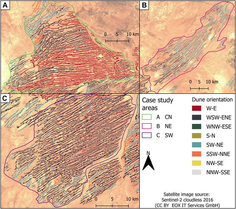
FIGURE 3. Map showing dune orientation in case study area CN (A), NE (B) and SW (C). Numerical class angles can be obtained from Supplementary Figure S10.
2.3.3 Dune junctions
The mapping of dune junctions is somewhat more complicated than for the other morphologic parameters. Previous studies of dune junction density have relied either on subjective, manual digitization of individual features (Bullard et al., 1995; Fitzsimmons, 2007) or resource-intensive deep learning approaches (Shumack et al., 2020), both of which we preferred to avoid in our open-source workflow. We therefore developed a new approach generalizing polygonal dune objects to line shapefiles by delineating the centre line of each dune polygon; this approach simultaneously captures the dune junctions, since they are defined by the merging of two dune crestal lines. We derived center lines from our multi-feature polygon shapefiles using the chordal axis tool from the geo-simplification toolbox in QGIS. This approach uses triangulation to calculate the center line according to the so-called Chordal Axis Transform (CAT) (Prasad, 2005). The calculated chordal axis depends on the quantity of neighboring triangles, whereby the chordal axis is defined as the perpendicular to the contact side of the adjacent triangles (Supplementary Figures S4, S5). All polygons with direct contact with neighboring polygons were manually corrected using the vertex digitizing tool; 224 of the 3,416 input polygons were corrected in this manner.
Once the polygons were corrected, we proceeded with manual mapping of junctions by creating point shapefiles with a point on each chordal axis intersection. We visually assessed the conformity of this approach with the satellite imagery for quality control and analyzed the results with the Nearest Neighbor Analysis, a visual interpretation of the spatial distribution of the junctions on density plots and spatial Kernel Density Estimates.
The Nearest Neighbor Analysis (NNA) allows to test the observed spatial distribution of point patterns, here junctions, against a hypothetical random distribution (Clark and Evans, 1954). The Nearest Neighbor Index is the ratio of the observed and expected mean distances and takes values NNI < 1 when the observed pattern is clustered and values NNI > 1 when it is dispersed (see Supplementary Figure S13). Both might indicate underlying spatial processes, in contrast to values around 1, which indicates a random distribution. The significance of this observation can be tested using z-values, where negative values indicate clustering and positive dispersion. The analysis was computed with the Tool “Nearest Neighbor Analysis” in the “Visualist” plugin for QGIS.
The spatial distribution of the junctions was then analyzed for junction density across the case study areas. Here we reprojected junction coordinates onto a profile line parallel to the mean dune orientation for a given area (for further details, see Supplementary Figures S6–S8). We reprojected the junction coordinates using a Python script (Perez and Granger, 2007) (script is cached at zenodo) which plotted the input data as a scatter plot including the profile line (see Supplementary Figures S10–S12). The script then shifted the origin of the coordinate system to the base (southwest-most) point of the profile line, so creating a new grid without coordinates but providing distance of each junction from the base point in meters (see Supplementary Figure S9). The data array output from this script was then loaded as Cartesian coordinates into R Studio, within which we generated a junction density plot as a topographic cross-section (Figure 5) to facilitate comparison between the case study areas using an R script (cached at zenodo).
We created a heatmap of dune junctions for each case study area in addition to the density plots. Heatmaps are kernel density estimations and facilitate visual identification of densities of a given feature (in this case, dune junctions). Suitable bandwidths for kernel size were estimated for each study area individually based on Silverman’s rule of thumb (Silverman, 1986) These were used to compute the Kernel Density Estimates with the QGIS Tool “Heatmap” using a quartic kernel shape [The raster dataset was then displayed as a map using a color ramp (Figure 6)].
2.3.4 Dune spacing
The mapping and measurement of dune spacing—defined here as the distance between dune crests—is complex due to the often non-parallel and non-uniform alignment between individual bedforms. The analysis of dune spacing over a dunefield must make assumptions relating to how the variation in distance between two dunes longitudinally should be treated; how different spacing lengths between the same two dunes should be weighted; and how dune junctions should be incorporated into the spacing measurements. Our workflow was designed to represent a compromise between efficiency and natural variability in the landforms. As yet, there are no GIS tools suited to semi-automatic measurement of dune spacing, and therefore we decided to undertake manual mapping for this component of the study.
Each case study area was too large to manually map all dune distances and therefore we undertook the measurements within randomly distributed grids in a more thorough adaptation of a previously published approach (Fitzsimmons, 2007). After creating line shapefiles with distance measured in meters, we placed 20–25, 5x1 km rectangular grids oriented perpendicular to the dune longitudinal axes using randomly generated central points retained in a point shapefile, from which the rectangles were extrapolated. The QGIS tool “rectangles, ovals, diamonds” allowed the orientation of the rectangle long axes to be rotated according to the mean dune orientation at the central point. Dune center lines were derived from the CAT (Section 2.3.3) and used as the start and end points of each dune spacing measurement (see Supplementary Figure S14). Five spacing measurements between two dune crests were obtained from each rectangle to ensure equal weighting of the measured distances. The length of each spacing measurement was determined using the QGIS field calculator to the nearest meter. Inter-dune distances were then imported and plotted in R Studio as both boxplots and histograms (the latter in both linear and log space) for each case study area. We used the Shapiro-Wilk Test (Shapiro and Wilk, 1965) to investigate whether spacing data were normally distributed.
2.3.5 Accuracy assessment
We validated the dune classification resulting from our GEOBIA approach against high-resolution satellite data in Google Maps. Since the segmentation results in a mapping of the “dune” and “non-dune” classes, we use the method of Fitzpatrick-Lins (1981) to determine the sample size, based on binomial probability theory. Accordingly, the recommended sample size is N = 204 points, assuming an expected accuracy of 85% and an allowable error of 5%. The points were distributed in the study areas according to a random sampling scheme. Their class was then determined visually using optical high-resolution satellite data and compared with the predicted values of our model. Compared to in-situ validation, our approach is much more cost- and resource-efficient, and since the resolution of the high-resolution satellite data exceeds the resolution of the terrain model by a factor of 10–30, it is still reasonably accurate. A confusion matrix was calculated from the value pairs of observed and predicted classes, which was used to determine the following quality indicators: producer’s and user’s accuracy, omission and commission error, overall accuracy, and the Kappa Coefficient of Agreement (Congalton and Green, 2009).
The conducted Accuracy Assessment (see Table 1) resulted in a Producer’s Accuracy of 89.9% for the class “dune” and 88.4% for class “non-dune.” User’s Accuracy for class “dune” was calculated to 71.0%, class “non-dune” to 96.5%. Therefore, overall classification quality of the methodology is high (Jensen, 2015, p. 569). The User’s Accuracy of class “dune” suggests a slight overprediction of dunes, likely as a result of issues with visual identification of non-vegetated-dunes. The Error of Omission was determined to be 10.2% for class “dune” and 11.6% for class “non-dune.” The Error of Commission for “dune” is at 29.0% and 3.5% for class “non-dune.” Those values result in an Overall Accuracy of 88.7% which seems solid respecting the given elevation data. The Kappa Coefficient of Agreement was calculated to 71.7% with an expected value of 60.2%. The Kappa statistics show that our model improves classification by 71.7% compared to a random classification and represents a substantial agreement (Jensen, 2015) between observed and predicted dune classes.
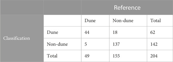
TABLE 1. Confusion Matrix associated with dune classification data.
3 Results
3.1 Dunefield morphological parameters
The overall dominant dune orientation for the dunefield–some 75% of all dune bedforms - lies along a WSW-ENE axis. Variation within individual case study areas, as well as for the entire region, is illustrated in Figure 4. Table 2 summarizes the main dune orientation statistics.
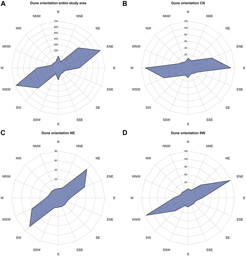
FIGURE 4. Dune rose diagrams for overall study area (A), case study area CN (B), NE (C) and SW (D) derived from dune orientation data.
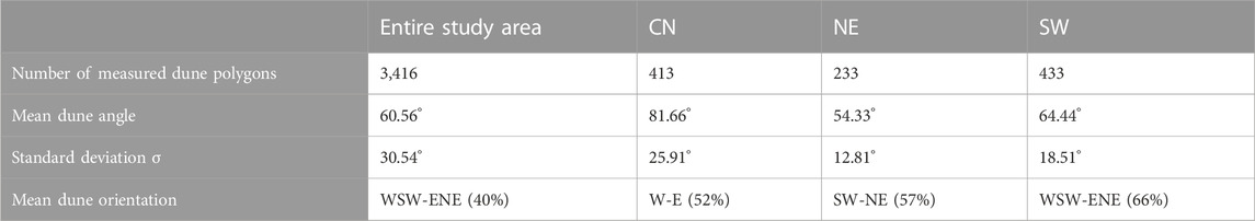
TABLE 2. Properties and statistics of dune orientation.
The northernmost case study area comprises dunes predominantly oriented SSW-NNE and is distinct from the rest of the region (Supplementary Figure S2A). The divergence in orientation of the northern area compared with the rest of the dunefield is visible in a comparison of the dune roses and in the small proportion of NNE-oriented dunes within the overall dune rose (Figure 4A). It is important to note here the prominent north-south escarpment of the Davenport Range on the eastern margins of this area, which rises 140 m above the main dunefield and potentially represents a topographic barrier to longitudinal dune migration.
3.2 Dune orientations
The CN case study area, immediately to the south of the north area, is dominated by W-E oriented dunes. Nevertheless, some variability in orientation is observed within this sub-region: the northern and southern parts of the case study area exhibit more WSW-ENE axes. The variation within this area is visible in the wider distribution of its dune rose (Figure 4B). The CN case study area also hosts a larger proportion of non-linear dunes and poorly defined hummocky bedforms than the others investigated. This may contribute to systematic error in the dune orientation analyses through the generation of unrealistic, oversized polygons in the classification process, which were then classified as single dunes with single orientations that do not reflect the true morphology. This error was observed in several cases, particularly in the western part of the CN case study area. The result is likely to be an underestimation of the proportion of WSW-ENE oriented dunes. We also observe a north-south oriented depression (in the form of several small playas) in the western part of the CN case study area, and an SSE-NNW oriented ridge through the centre of the area which rises up to 40 vertical meters above the depressions in the west (Figure 5B). The Davenport Range rises up to 230 vertical meters above the CN part of the dunefield on its northeastern margins. We will discuss the potential influence of these topographic anomalies on dune orientation in Section 4.2.

FIGURE 5. Density plots (red) and cross profile plots (black) for case study area CN (A,B), NE (C,D) and SW (E,F). Showing the dune junction distribution from the predominant dune orientation direction, in comparison to the respective topographic profile. Topographic and reprojection profile line are plotted in Supplementary Figure S15.
The NE case study area hosts the most of linear dunes, with a dominant SW-NE orientation and a secondary WSW-ENE axis (Figure 4C). Two narrow north-south ridges overlain by dunes rise c. 20 vertical meters above the surrounding underlying relief and straddle a small playa in the south-western part of the NE case study area (Figure 3B). North-eastwards, the underlying topography slopes gently down to the Kati Thanda shoreline. This case study area appears to be the most suited to our workflow due to the morphology, size, spacing and length of the dunes.
The SW case study area yields the least variability in dune orientation of the subregions analyzed. Almost 75% of the dunes in this area are oriented WSW-ENE (Figure 4D). However, a number of hummocky dunes in this area generate small polygons which do not follow the main dune orientation, so yielding a wider distribution of orientations in the resulting dune rose than the NE case study area but one less variable than observed in the CN case study area. The central and northeastern parts of this subregion host clearly linear dune forms, with less well defined, hummocky forms more common in the western quadrant (Figure 3C).
3.3 Dune junctions
The spatial distribution and density of linear dune junctions may relate to aeolian transport and sediment supply (Wasson and Hyde, 1983; Wasson et al., 1988), as well as interaction with underlying topography and non-aeolian landforms (Fitzsimmons, 2007). We concede that our study focusses on a region of vegetated linear dunes, and therefore cannot comment on whether dune junctions such as these also occur in unvegetated regions; nevertheless, the tools for mapping are applicable anywhere. In order to investigate these possible influences on dune planform, we present the data both as cross-sections of dune junction density, overlain on the topographic profiles along the mean longitudinal axis for each case study area (Figure 5), and as heatmaps of junction density overlain on the satellite imagery (Figure 6).
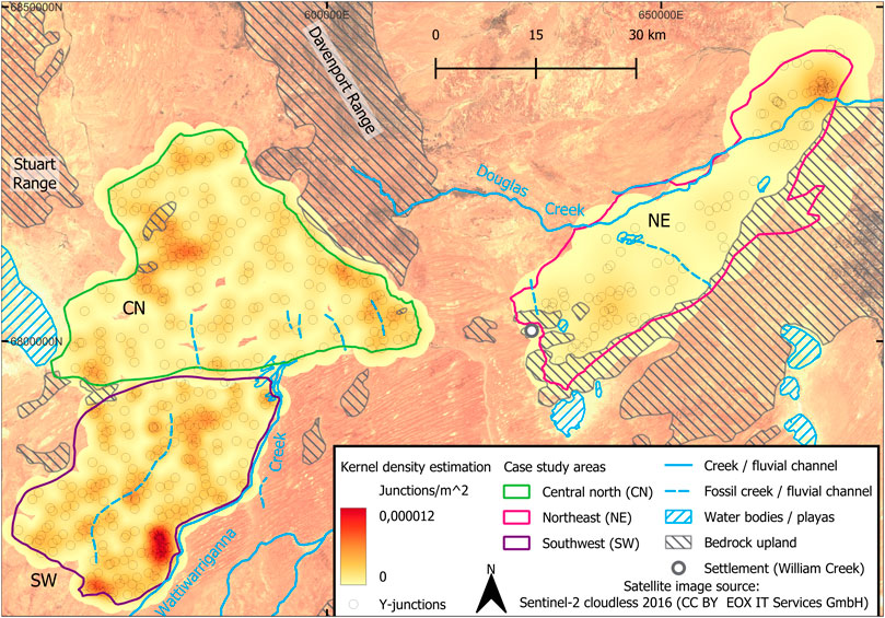
FIGURE 6. Heatmaps depicting results of kernel density estimation for case study areas.
The results of our Nearest Neighbor Analysis show, that all study areas have index values below NNI < 1 and therefore the observed mean distances are shorter than expected random distances. This indicates clustering of junctions. The z-values are lower than a significance threshold of z < −2.58 (p < 0.01), highlighting that the pattern of junctions differs significantly from a random distribution (Table 3).
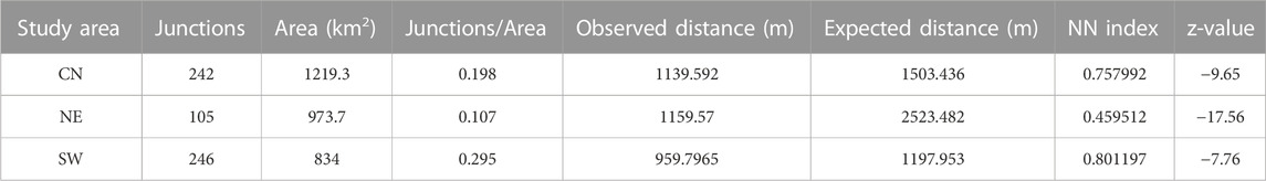
TABLE 3. Table showing properties of dune Y-junctions in several case study areas needed for creating kernel density heatmaps.
The NE case study area exhibits the lowest density of dune junctions. We mapped 105 junctions across the 973.7 km2 area, resulting in a mean density of 0.107 junctions per km2. Two peaks in dune junction frequency can be observed along our reprojected transect, occurring in the west at c. 10 km and in the east at c. 45 km (Figure 6C). The western quadrant peak in junction frequency corresponds to a topographic high, whereas the eastern peak occurs in a low elevation, low relief area. The kernel density heatmaps indicate a cluster of dune junctions in the northeastern corner of the subregion (Figure 6B).
The CN case study area contains an intermediate density of dune junctions; 242 junctions were mapped onto an area of 1,219.3 km2, resulting in a mean density of 0.198 junctions per km2. The highest concentration of dune junctions occurs at c. 15 km along the reprojection line (Figures 5A, 6A), which corresponds to the west-facing mid-slope of the underlying topography. We observe an additional, minor cluster of junctions at c. 44 km on the eastern margins of the CN case study area (Figures 5A, 6A). There is no clear correlation at this location with the underlying topography just to the west of the topographic ridge, which is likely to correspond to the 15 km cluster observed in our reprojected transects (Figure 5A). Another cluster is located on the eastern margins of the CN case study area—correlating with the 44 km peak—in the vicinity of the transition between dunes and the Davenport Range to the east.
The highest density of dune junctions can be observed in the SW case study area. In this area, we mapped 246 junctions over an area of 833 km2, resulting in a mean density of 0.295 junctions per square kilometer. The SW case study area is underlain by more variable topography than the other two case study areas; three topographic highs and three topographic lows occur along the 45 km reprojected transect (Figure 5F). The dune junction density is highest at c. 20 km along the transect (Figure 5E), which corresponds to a zone of higher elevation. Our kernel density heatmap highlights a cluster of junctions on the southern margins of the SW case study area (Figure 6C), adjacent the Wattiwarriganna Creek bed, only when the radius size is increased to values where it is questionable whether a resulting cluster would be meaningful.
3.4 Dune spacing
The spacing distances between linear dunes may relate to sediment availability, underlying substrate material (which may or may not be associated with sediment availability), vegetation cover, wind capacity, drift potential and interactions between dune bedforms and underlying topography or proximal non-aeolian landforms (Wasson et al., 1988; Hesse and Simpson, 2006; Hollands et al., 2006; Fitzsimmons, 2007; Fitzsimmons et al., 2020). Although the measurement of dune spacing was challenging due to the strong dependence on the assumptions described in Section 2.3.4, we nevertheless observe geographical variability in dune spacing characteristics. The results of our dune spacing measurements for the three case study areas are summarized in Table 4.
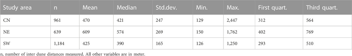
TABLE 4. Statistic properties of inter-dune spacing in the three case study areas.
We present the distribution of dune spacing for the respective case study areas as box plots and a raincloud plot in Figure 7. We observe a number of differences in spacing characteristics between the case study areas. Both the mean and median dune spacing values for the CN case study area are intermediate (470 m and 421 m, respectively), but with a high standard deviation indicating variable spacing across the area. The CN case study area also hosts dune pairs with the widest spacing observed in the dunefield (2,447 m). By contrast, the NE area contains the largest mean distance between dune pairs (609 m), although this area has the largest standard deviation of the three areas studied (269 m). The SW case study area hosts the shortest mean spacing (425 m) and smallest standard deviation (165 m); the largest number of short inter-dune distances are found in this area. Overall, however, the mean spacing and their standard deviations are similar between the CN and SW case study areas; the main difference in spacing characteristics for these two areas lie in the occurrence of dune pairs spaced very far apart in the CN area. Most dunes are spaced between 300 and 500 m apart across all three case study areas and are distributed normally around this peak when a logarithmic scale is used for the spacing distance.
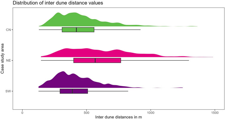
FIGURE 7. Raincloud plot showing results of inter dune spacing data acquisition. Displayed for each study area.
4 Discussion
4.1 A workflow for dunefield mapping using open-source GIS
We consider the workflow developed in this study to be effective for mapping dunefields and extracting morphological data on linear dune bedforms. Nevertheless, some improvements could be made to increase efficiency and improve accuracy. Here we assess our workflow and suggest possible changes for future studies.
Given our emphasis on an open-source approach, we consider the primary datasets used and their preprocessing to represent the optimal compromise between resolution and accessibility. The vertical precision of our primary data represents a limiting factor to our workflow, particularly given the low relief of the study region. Although Light Imaging Detection And Ranging (LIDAR) data would improve the resolution of our spatial analysis (Florinsky, 2016; Solazzo et al., 2018; Dong et al., 2021), there are as yet no free-to-use datasets covering our study area. Furthermore, LIDAR processing is computationally intensive and increases the costs for hardware and runtime for researchers. The DSM used in our study, with 27.5 m spatial resolution, represents the best possible compromise for our open-source approach. The UTM coordinate system is a convenient choice for mapping at a regional scale with study areas less than ∼1,000 km wide, as it combines high horizontal accuracy with metric coordinates and global applicability. Visual inspection of our output data confirmed that our GEOBIA approach based on the segmentation of a low-pass filtered DSM using thresholds and areal object parameters produces the best possible result. The accuracy of dune polygons is most dependent on the classification threshold values, since these determine the resultant dune maps and morphologic data. We argue that the values used in this study are optimal for this region in order to find the balance between reducing the data sufficiently to easily identify and remove irrelevant features, while not losing too many pixels which carry dune-related information. The low pass filter is scale-dependent and varies with the magnitude of dune size and kernel, so that these values are specific to the dunefield studied and should be calibrated to local conditions for future studies in other regions.
Our measurements of dune orientation were strongly dependent on the size and accuracy of the segment polygons, which were generated using the threshold values determined during preprocessing. The classification assumptions described in Section 2.3.1 resulted in the production of a number of very large polygons with multiple longitudinal axes, particularly in the CN case study area. Such polygons could only be rectified into individual dune forms by time-consuming manual division into smaller polygons, or by accepting lower accuracy in the analysis of orientation statistics. Again, the balance must be struck between efficiency and accuracy given the scale of the area to be mapped. Visual inspection of our results indicates an acceptable degree of accuracy, although this should always be assessed in the context of the research question and scale. Our approach to derive the angles of polygon longitudinal axes using the available QGIS script was effective, although the implementation of the data in R could be improved with further script development.
One disadvantage of our proposed workflow is the substantial effort involved in generating dune junction statistics. Although the use of chordal axis intersections produces an accurate dataset of dune junctions, it is debatable whether this is the right approach for this particular dunefield given its subdued topography and unquantifiable sediment supply without ground truthing. The low relief of the southwest Kati Thanda (Lake Eyre) dunefield prevents an effective classification of dune height thresholds and requires intensive manual correction of dune polygons both to run the CAT and to map junctions according to chordal axis intersections. The “blurring” effect of low relief dunes results in artificially large polygons which affects the CAT triangulation process. In the context of our study region, this process could really only be improved by developing better reclassification thresholds or more manual correction of the output data. However, our approach would be effective in regions with greater topographic relief. Finally, we assess the reprojection of the density plots to be an effective means of obtaining information relating junction densities with underlying topography, and by proxy, interactions between dunes and other landforms.
We argue that our approach to measuring dune spacing could be improved. Our method not only requires substantial manual effort, but also has a strong dependence on the location of the measurement lines relative to the dune central axes. This can result in systematic error, although we concede that over the scale of the dunefield studied, the overall errors may not be so large as to compromise accuracy. Interdune distance measurements may be improved using the “Hausdorff distance”, which measures the mean distance between two polygons (Alt et al., 2003) and can be undertaken using the QGIS field calculator. Developing a semi-automated method for measuring the “Hausdorff distance” would however require substantial effort to implement.
Overall, we argue that open-source GIS, such as SAGA and QGIS, can be effectively used in a workflow to extract meaningful information from spatial terrain data. The precision of our output is sufficiently high to extract dune-related data despite the significant challenge of low topographic relief; for other dunefields with higher dune bedforms and greater topographic relief, the workflow developed here would be even more effective. The widespread adoption of our open-source workflow will hopefully make meaningful assessments of dunefield morphologic variability as a framework for larger questions relating to dunefield expansion more accessible to our colleagues with fewer financial resources.
4.2 Links between dunefield morphologic variability, wind regime, topography and non-aeolian landforms
The orientation data for the SW Kati Thanda (Lake Eyre) dunefield provides us with an opportunity to investigate the degree to which linear dune orientations represent a response to factors additional to wind regimes, such as topographic and geomorphic barriers. We recognize that dunefields are composite landscapes comprising individual landforms which may not have been active all at the same time (Hesse and Simpson, 2006; Fitzsimmons, 2007; Fitzsimmons et al., 2013) and our interpretation is thereby limited, since we do not have the temporal perspective. Compared with linear dunefields elsewhere across Australia (Jennings, 1968; Hesse, 2010), the SW Kati Thanda (Lake Eyre) dunefield exhibits substantial variability in dune orientation across a relatively small area (Figure 3). Fundamental to our interpretations here is the assumption that dune orientations represent formation parallel to the resultant sand-shifting wind vector at the time of formation (Tsoar, 1989). Based on a comparison with less topographically diverse adjacent dunefields (the Victoria to the west and Tirari to the east (Hesse, 2010), we can expect our study region to translate to a zone of transition from westerly winds in the southern part to winds with a more south-westerly component in the northern part. We observe a substantial swing in linear dune orientation in the northern half of our area in the proximity of the Davenport Range which rises 140 vertical meters above the dunefields, where we might expect a SW-NE (bearing 45°) dune orientation if there were no topographic barriers. In fact, we observe a mean linear dune orientation of 46° in the northernmost part, which diverges only 1° from the hypothesized 45° bearing. Dunes in this northernmost area occur in a c. 20 km wide plain between the Davenport Range to the east and the Stuart Range escarpment to the west of roughly the same height. We propose this divergence from the hypothesized non-topographically influenced dune orientation to be a response of the dunes to surrounding topography, due to the deflection of near-surface winds by the uplands northwards along the axis of the main escarpments (Fitzsimmons et al., 2020). We also observe a shift in mean dune orientation in the CN case study area which lies immediately southwest of the Davenport Range. In the case of CN, it is not the entire dunefield which is deflected; rather there is a net orientation change in the dunes of 22.5°, from a mean WNW-ESE orientation shifting to W-E. This transition starts 27 km west (and therefore upwind) of the Davenport Range. The dunes terminate on the windward side of an ephemeral channel at the base of the escarpment. We therefore hypothesize that the orientation of linear dunes, as an approximate proxy for near-surface sand-shifting winds, are affected by topographic uplands through the deflection of air masses and thereby aeolian transport along an escarpment. This effect would appear to initiate some distance upwind (in this case 27 km) from the topographic barrier. That distance may be proportional to the height (and possibly slope angle) of the topographic barrier, but is beyond the scope of this study to define more precisely. Shifts in dune orientation relating to nearby topographic highs have previously been subjectively observed in Australia (Hollands et al., 2006) and Central Asia (Fitzsimmons et al., 2020); the data from our study provides the first opportunity to investigate this phenomenon in a semi-quantitative way. Although there are differences in vertical relief of up to 40 m across the dunefield, we do not observe any substantial, sudden shifts in orientation on the order of what we observe near the Davenport Range. We also observe no substantial change in dune orientation relating to the occurrence of ephemeral creeks or playas, which form gentle depressions in the landscape and another potential barrier to aeolian transport (Wopfner and Twidale, 1988). We therefore infer that the topography beneath the dunefield is insufficiently high or steep to deflect the near-surface winds and alter the dune orientation; rather the more gradual change in orientation is likely to relate to the synoptic-scale changes in wind regimes which are believed to be responsible for the continental-scale dune whorl (Wasson and Hyde, 1983; Hesse, 2010).
Our analysis of the distribution and frequency of linear dune junctions across the dunefield was undertaken with the aim of investigating possible interactions with underlying topography, non-aeolian landform types, and by extension, local sediment supply. Until recently, dune junctions have been largely overlooked as a source of information about large-scale dunefield formation, in part due to technical difficulties of quantifying these features over large scales [e.g., (Fitzsimmons, 2007)]. Recent work using deep-learning approaches produced data in the form of junctions per kilometer of dune crest in the Simpson, Strzelecki and Mallee dunefields in Australia (Shumack et al., 2020). Unfortunately, however, our workflow prevented directly comparable data and therefore we cannot put our own results into the wider perspective of dunefields across the continent. Nevertheless, our dataset highlights some potential external influences on dune morphology.
The increase in dune junction density at c. 15 km along our longitudinal transect for the CN case study area coincides with a topographic ridge which runs perpendicular to the main dune axis. Visual inspection of the dunes in this locality shows that the dunes are also less linear and more sinuous. The reduction in linearity and increase in dune junctions may have several explanations: 1) there is less available sediment on the ridge slope, which has a more shallow sediment cover, so requiring the bedforms to merge with one another in a form of sediment economization; 2) the ridge slope would require higher kinetic energy to transport sand uphill, resulting in further economization of sediment on the slope; 3) the presence of the Sturt and Davenport Ranges on either side of the CN area may create more turbulent, multi-directional wind flow at this point which may redirect the aeolian bedforms and create junctions. We suggest the latter case to be the least likely, since there is no reason to assume that the near-surface wind regime would become more turbulent at the 15 km point than anywhere else between the two ranges. It is feasible that an interplay between the first two hypotheses explains the higher density of dune junctions at this locality. At this stage, however, it is difficult to prove these theories due to the limitations in the resolution of the underlying DSM to fully characterize the terrain on the ridge, and in the lack of freely available geophysical data providing information about sediment cover thickness on the ridge. Comparing the junction density results with dune spacing at this locality–another parameter which may reflect sediment supply (Wasson and Hyde, 1983; Fitzsimmons, 2007; Lancaster, 2009)—may help us interrogate the mechanisms involved. It is interesting to note a reduction in junction frequency on the ridge peak; if we invoke the first two arguments above, then perhaps the dunes by this stage have exhausted sediment supply to the point where no further merging is possible. In any case, these arguments indicate a degree of longitudinal migration of the linear dune forms; perhaps not as elongated as originally proposed by (Twidale, 1968; Twidale, 1972) but more than the local sand supply model proposed by (King, 1960). An additional cluster of junctions occurs on the northeastern margins of the CN case study area, at the juxtaposition with the Davenport Range and with an ephemeral peak at the base of the escarpment. The merging dune forms at this point provide additional support for the longitudinal migration model, since they appear to be merging in response to a geomorphic (the creek) or topographic (the escarpment) barrier impeding further migration.
In other localities, peaks in dune junction density coincide with non-aeolian landforms such as ephemeral creeks and chains of playas. Since these represent topographic lows, but also possible sources of sediment, we must examine the context in order to hypothesize which of the two possible influences are the greater. We observe increased junction frequency to the west of William Creek in the NE case study area, on the northeastern margins of the same where the Douglas Creek cuts through the dunefield, and in the central section where a chain of playa depressions underlies the dunefield (Krapf et al., 2018). In the SW case study area we observe more frequent dune junctions on the western bank of the Wattiwarriganna Creek. In these cases, the increase in dune junctions occurs upwind of the respective geomorphic features (Bowler, 1976), and may reflect a relative decrease in sediment supply as the underlying substrate provides less available sand for transport in a downwind direction (Goudie and Middleton, 2006; Fitzsimmons, 2007).
There is an overall lack of dune spacing data globally with which to assess our dune spacing results; what data do exist, are often in different forms (Ewing and Kocurek, 2010; Fitzsimmons, 2007; others) and do prevent direct comparison between dunefields. Previous work nevertheless suggests that dune spacing is closely related to local sediment supply (Fitzsimmons, 2007); others), whether through active sediment input from fluvial channels or a lack of available sand-sized material for entrainment over stony pavements and clay-rich playas. In this study, we observe generally more closely spaced dunes in the SW and CN case study areas than in the NE. Visual inspection of underlying geomorphic features, which may provide information about sediment availability, suggests that sediment supply may have driven the larger interdune distances in the NE, since this area overlies both stony pavement and a larger proportion of area covered by playas than observed in the other two areas. In addition, the Wattiwarriganna Creek cuts through the SW and CN areas, and a number of probable fossil abandoned creeks underlie these areas. These features are likely to have provided sediment supply, whether by active input downwind of active channel banks or the presence of unconsolidated sandy substrate. As such, there is a range of mechanisms by which the aeolian dunes may interact with fluvial systems, and which have an influence on their morphological characteristics.
Dune junctions and inter-dune spacing are inversely proportional in all three case study areas. Area SW shows the highest number of junctions and the lowest mean inter-dune distances. NE shows the lowest counts in junctions and the highest mean inter-dune distance. CE lies in both categories in the middle. Tests on statistical significance or correlations between both categories have not been made. This would be a subject of interest for future research on a potential interaction between both categories. The observed non-normal distribution (all α 5% significance) of the values indicates either a random mechanism of inter-dune distancing or a methodology containing (systematic/measure) errors.
Arguably, the interaction between dunes, topography and on aeolian landforms is best examined by considering the parameters in concert. For example, there are localities where we observe an increase in dune junction frequency and a decrease in interdune spacing, and vice versa. Qualitatively, the SW Kati Thanda (Lake Eyre) dunefield appears to have more instances where dune junction density and spacing values increase, which we propose may relate to the role both of underlying and surrounding topography as physical barriers to dune migration. Applying our workflow to dunefields with less geomorphic variability over a small area may yield contrasting insights, indicating different mechanisms such as sediment supply or reduction thereof, deflection of wind regimes by the surrounding relief, or underlying topography influencing the kinetic energy required to transport the sand up or down slopes. Our results provide some first insights and hypotheses into the nature of these interactions, and despite their limitations can nevertheless be considered to advance the state of knowledge of large-scale dunefield dynamics.
Data availability statement
The datasets presented in this study can be found in online repositories. The names of the repository/repositories and accession number(s) can be found in the article/Supplementary Material.
Author contributions
LF, CS, and KF contributed to the conception and design of the study. LF and CS designed the GIS workflow and developed the methodology. LF and KF undertook the geomorphic analysis. LF wrote the first draft of the manuscript. All authors contributed to the article and approved the submitted version
Acknowledgments
We wish firstly to acknowledge the deep and continued connection held by the Arabuna First Nations people to Country around Kati Thanda. We also thank the Terrestrial Sedimentology Group at the Department of Geosciences, University of Tübingen for feedback during the development of this project, in particular P. Gewalt who provided helpful statistical advice which assisted with the data visualization. Furthermore, we thank the working group of Volker Hochschild (Physical Geography and Geoinformatics) at the Department of Geography, University of Tuebingen and the Heidelberg Academy of Sciences and Humanities for funding the research project “The Role of Culture in Early Expansions of Humans.”
Conflict of interest
The authors declare that the research was conducted in the absence of any commercial or financial relationships that could be construed as a potential conflict of interest.
Publisher’s note
All claims expressed in this article are solely those of the authors and do not necessarily represent those of their affiliated organizations, or those of the publisher, the editors and the reviewers. Any product that may be evaluated in this article, or claim that may be made by its manufacturer, is not guaranteed or endorsed by the publisher.
Supplementary material
The Supplementary Material for this article can be found online at: https://www.frontiersin.org/articles/10.3389/feart.2023.1196244/full#supplementary-material
Supplementary Figure S1 | Map showing the classification result in blue polygons (left) compared to a Sentinel 2 satellite image (right) of the same location.
Supplementary Figure S2 | Dune rose diagrams for case study area N (A) and S (B) derived from dune orientation data.
Supplementary Figure S3 | Script from the QGIS field calculator to calculate dune orientation from Polygon orientations within the range of 0°–180°.
Supplementary Figure S4 | Triangulation method for creating chordal axis (blue line and blue dashed line) out of neighboring triangles. (A) No neighboring triangle. (B) One neighboring triangle. (C) Two neighboring triangles. (D) Three neighboring triangles.
Supplementary Figure S5 | Map of the study area showing methodology of CAT.
Supplementary Figure S6 | Input point data for reprojected density plots with profile line in case study area CN.
Supplementary Figure S7 | Input point data for reprojected density plots with profile line in case study area NE.
Supplementary Figure S8 | Input point data for reprojected density plots with profile line in case study area SW.
Supplementary Figure S9 | Reprojection methodology for density plots.
Supplementary Figure S10 | Output point data for reprojected density plots with profile line in case study area CN.
Supplementary Figure S11 | Output point data for reprojected density plots with profile line in case study area NE.
Supplementary Figure S12 | Output point data for reprojected density plots with profile line in case study area SW.
Supplementary Figure S13 | Methodology of calculating the Nearest Neighbor Analysis (NNA) after Clark and Evans (1954).
Supplementary Figure S14 | Map of the study area showing the methodology of measuring inter-dune distances.
Supplementary Figure S15 | Map of the study area showing the input digital elevation data as well as the location of the topographic profile lines and reprojected profile lines for reprojecting dune junction points.
References
Al-Masrahy, M. A., and Mountney, N. P. (2015). A classification scheme for fluvial–aeolian system interaction in desert-margin settings. Aeolian Res. 17, 67–88. doi:10.1016/j.aeolia.2015.01.010
Alley, N. F. (1998). Cainozoic stratigraphy, palaeoenvironments and geological evolution of the Lake Eyre Basin. Palaeogeogr. Palaeoclimatol. Palaeoecol. 144, 239–263. doi:10.1016/s0031-0182(98)00120-5
Alt, H., Acosta, M. D., and Gill, T. E. (2003). “Computing the hausdorff distance of geometric patterns and shapes,” in Discrete and computational geometry: The goodman-pollack festschrift. Editors B. Aronov, S. Basu, J. Pach, and M. Sharir (Berlin(Heidelberg): Springer), 65–76.
Armon, M., Dente, E., Shmilovitz, Y., Mushkin, A., Cohen, T., Morin, E., et al. (2020). Determining bathymetry of shallow and ephemeral desert lakes using satellite imagery and altimetry. Geophys. Res. Lett. 47, e2020GL087367. doi:10.1029/2020gl087367
Baddock, M. C., Bryant, R. G., Acosta, M. D., and Gill, T. E. (2021). Understanding dust sources through remote sensing: Making a case for CubeSats. J. Arid Environ. 184, 104335. doi:10.1016/j.jaridenv.2020.104335
Bailey, R. M., and Thomas, D. S. G. (2014). A quantitative approach to understanding dated dune stratigraphies. Earth Surf. Process. Landforms 39, 614–631. doi:10.1002/esp.3471
Blaschke, T., Hay, G. J., Kelly, M., Lang, S., Hofmann, P., Addink, E., et al. (2014). Geographic object-based image analysis – towards a new paradigm. ISPRS J. Photogrammetry Remote Sens. 87, 180–191. doi:10.1016/j.isprsjprs.2013.09.014
Boucaut, W. R. P., Dunstan, N. C., Krieg, G. W., and Smith, P. C. (1986). The geology and hydrogeology of the Dalhousie Springs. Witjira National Park: Report Book, 13.
Bowler, J. M. (1976). Aridity in Australia: Age, origins and expression in aeolian landforms and sediments. Earth-Science Rev. 12, 279–310. doi:10.1016/0012-8252(76)90008-8
Breed, C. S., and Grow, T. (1979). Morphology and distribution of dunes in sand seas observed by remote sensing. A study Glob. sand seas 1052, 253–302.
Bristow, C. S., Augustinus, P., Wallis, I., Jol, H., and Rhodes, E. (2010). Investigation of the age and migration of reversing dunes in Antarctica using GPR and OSL, with implications for GPR on Mars. Earth Planet. Sci. Lett. 289, 30–42. doi:10.1016/j.epsl.2009.10.026
Bristow, C. S., Bailey, S. D., and Lancaster, N. (2000). The sedimentary structure of linear sand dunes. Nature 406, 56–59. doi:10.1038/35017536
Bullard, J. E., Thomas, D. S. G., Livingstone, I., and Wiggs, G. F. S. (1995). Analysis of linear sand dune morphological variability, southwestern Kalahari desert. Geomorphology 11, 189–203. doi:10.1016/0169-555x(94)00061-u
Chen, G., Weng, Q., Hay, G. J., and He, Y. (2018). Geographic object-based image analysis (GEOBIA): Emerging trends and future opportunities. GIScience Remote Sens. 55, 159–182. doi:10.1080/15481603.2018.1426092
Clark, P. J., and Evans, F. C. (1954). Distance to nearest neighbor as a measure of spatial relationships in populations. Ecology 35, 445–453. doi:10.2307/1931034
Congalton, R. G., and Green, K. (2009). Assessing the accuracy of remotely sensed data: Principles and practices. 2nd Ed. Boca Raton: CRC Press.
Conrad, O., Bechtel, B., Bock, M., Dietrich, H., Fischer, E., Gerlitz, L., et al. (2015). System for automated geoscientific analyses (SAGA) v. 2.1.4. Geosci. Model. Dev. 8, 1991–2007. doi:10.5194/gmd-8-1991-2015
Courrech du Pont, S., Narteau, C., and Gao, X. (2014). Two modes for dune orientation. Geology 42, 743–746. doi:10.1130/g35657.1
Courty, L. G., Soriano-Monzalvo, J. C., and Pedrozo-Acuña, A. (2019). Evaluation of open-access global digital elevation models (AW3D30, SRTM, and ASTER) for flood modelling purposes. J. Flood Risk Manag. 12, e12550. doi:10.1111/jfr3.12550
Cowley, W. M., Tily, L., and Irvine, J. A. (2020). Geological map south Australia, 1: 2 000 000 scale. s.l. Department for Energy and Mining.
Dong, P., Xia, J., Zhong, R., Zhao, Z., and Tan, S. (2021). A new method for automated measurement of sand dune migration based on multi-temporal LiDAR-derived digital elevation models. Remote Sens. 13, 3084. doi:10.3390/rs13163084
Drexel, J. F., Preiss, W. V., and Parker, A. J. (1995). “The geology of South Australia,” in Vol. 2: The phanerozoic. Adelaide: Mines and energy (South Australia: Geological Survey of South Australia).
Ewing, R. C., and Kocurek, G. A. (2010). Aeolian dune interactions and dune-field pattern formation: White sands dune field, new Mexico. Sedimentology 57, 1199–1219. doi:10.1111/j.1365-3091.2009.01143.x
Fitzpatrick-Lins, K. (1981). Comparison of sampling procedures and data analysis for a land-use and land-cover map. Photogrammetric Eng. Remote Sens. 47, 343–351.
Fitzsimmons, K. E., Cohen, T. J., Hesse, P. P., Jansen, J., Nanson, G. C., May, J. H., et al. (2013). Late Quaternary palaeoenvironmental change in the Australian drylands. Quat. Sci. Rev. 74, 78–96. doi:10.1016/j.quascirev.2012.09.007
Fitzsimmons, K. E. (2007). Morphological variability in the linear dunefields of the Strzelecki and Tirari deserts, Australia. Geomorphology 91, 146–160. doi:10.1016/j.geomorph.2007.02.004
Fitzsimmons, K. E., Nowatzki, M., Dave, A. K., and Harder, H. (2020). Intersections between wind regimes, topography and sediment supply: Perspectives from aeolian landforms in Central Asia. Palaeogeogr. Palaeoclimatol. Palaeoecol. 540, 109531. doi:10.1016/j.palaeo.2019.109531
Fitzsimmons, K. (2005). Oases in the desert: Mound springs and their role in desert hydrology. J. Virtual Explor. 20, 134. doi:10.3809/jvirtex.2005.00134
Fryberger, S. G., and Dean, G. (1979). “Dune forms and wind regime,” in A study of global sand seas (Washington: US Government Printing Office Washington), 137–169.
Fujioka, T., Chappell, J., Fifield, L. K., and Rhodes, E. J. (2009). Australian desert dune fields initiated with Pliocene–Pleistocene global climatic shift. Geology 37, 51–54. doi:10.1130/g25042a.1
Fujioka, T., Chappell, J., Honda, M., Yatsevich, I., Fifield, K., and Fabel, D. (2005). Global cooling initiated stony deserts in central Australia 2–4 Ma, dated by cosmogenic 21Ne-10Be. Geol. 33, 993–996. doi:10.1130/g21746.1
Gavrilov, M. B., Marković, S. B., Schaetzl, R. J., Tošić, I., Zeeden, C., Obreht, I., et al. (2018). Prevailing surface winds in Northern Serbia in the recent and past time periods; modern- and past dust deposition. Aeolian Res. 31, 117–129. doi:10.1016/j.aeolia.2017.07.008
Gholami, H., Mohammadifar, A., Malakooti, H., Esmaeilpour, Y., Golzari, S., Mohammadi, F., et al. (2021). Integrated modelling for mapping spatial sources of dust in central Asia - an important dust source in the global atmospheric system. Atmos. Pollut. Res. 12, 101173. doi:10.1016/j.apr.2021.101173
Goudie, A. S., and Middleton, N. J. (2006). Desert dust in the global system. Heidelberg(Germany): Springer Berlin Heidelberg.
Hesse, P. P., and Simpson, R. L. (2006). Variable vegetation cover and episodic sand movement on longitudinal desert sand dunes. Geomorphol. 81, 276–291. doi:10.1016/j.geomorph.2006.04.012
Hesse, P. P. (2010). The Australian desert dunefields: Formation and evolution in an old, flat, dry continent. Geol. Soc. Lond. Spec. Publ. 346, 141–164. doi:10.1144/sp346.9
Hollands, C. B., Nanson, G. C., Jones, B. G., Bristow, C. S., Price, D. M., and Pietsch, T. J. (2006). Aeolian–fluvial interaction: Evidence for late quaternary channel change and wind-rift linear dune formation in the northwestern Simpson desert, Australia. Quat. Sci. Rev. 25, 142–162. doi:10.1016/j.quascirev.2005.02.007
Huang, J., Li, Y., Fu, C., Chen, F., Fu, Q., Dai, A., et al. (2017). Dryland climate change: Recent progress and challenges. Rev. Geophys. 55, 719–778. doi:10.1002/2016rg000550
Huang, J., Yu, H., Guan, X., Wang, G., and Guo, R. (2016). Accelerated dryland expansion under climate change. Nat. Clim. Change 6, 166–171. doi:10.1038/nclimate2837
Hugenholtz, C. H., Levin, N., Barchyn, T. E., and Baddock, M. C. (2012). Remote sensing and spatial analysis of aeolian sand dunes: A review and outlook. Earth-Science Rev. 111, 319–334. doi:10.1016/j.earscirev.2011.11.006
Jennings, J. N. (1968). A revised map of the desert dunes op Australia. Aust. Geogr. 10, 408–409. doi:10.1080/00049186808702508
Jensen, J. R. (2015). Introductory digital image processing: A remote sensing perspective. 4th ed. USA: Prentice Hall Press.
Kazemi Garajeh, M., Feizizadeh, B., Weng, Q., Rezaei Moghaddam, M. H., and Kazemi Garajeh, A. (2022). Desert landform detection and mapping using a semi-automated object-based image analysis approach. J. Arid Environ. 199, 104721. doi:10.1016/j.jaridenv.2022.104721
King, D. (1960). The sand ridge deserts of South Australia and related aeolian landforms of the Quaternary arid cycles. Trans. R. Soc. S. Aust. 83, 99–108.
Koutroulis, A. G. (2019). Dryland changes under different levels of global warming. Sci. Total Environ. 655, 482–511. doi:10.1016/j.scitotenv.2018.11.215
Krapf, C. B. E., Lang, S. C., and Werner, M. (2022). The interplay of fluvial, lacustrine and aeolian deposition and erosion along the Neales Cliffs and its relevance to the evolution of Kati Thanda-Lake Eyre, central Australia, during the Quaternary. Trans. R. Soc. S. Aust. 146, 7–30. doi:10.1080/03721426.2022.2035199
Krapf, C. B. E., Stollhofen, H., and Stanistreet, I. G. (2003). Contrasting styles of ephemeral river systems and their interaction with dunes of the Skeleton Coast erg (Namibia). Quat. Int. 104, 41–52. doi:10.1016/s1040-6182(02)00134-9
Krapf, C., Keeling, J., and Petts, A. (2018). Cretes and ‘chemical’ landscapes, South Australia. Adelaide: Department of the Premier and Cabinet, 63.
Lancaster, N. (2009). “Dune morphology and dynamics,” in Geomorphology of desert environments. Editors A. J. Parsons, and A. D. Abrahams (Dordrecht: Springer Netherlands), 557–595.
Liu, B., and Coulthard, T. J. (2015). Mapping the interactions between rivers and sand dunes: Implications for fluvial and aeolian geomorphology. Geomorphology 231, 246–257. doi:10.1016/j.geomorph.2014.12.011
Longley, P. (2005). Geographical information systems and science. 2nd ed ed. Chichester Hoboken, NJ: Wiley.
Mabbutt, J. A. (1968). Aeolian landforms in central Australia. Aust. Geogr. Stud. 6, 139–150. doi:10.1111/j.1467-8470.1968.tb00185.x
Magee, J. W., Miller, G. H., Spooner, N. A., and Questiaux, D. (2004). Continuous 150 k.y. monsoon record from Lake Eyre, Australia: Insolation-forcing implications and unexpected Holocene failure. Geol. 32, 885–888. doi:10.1130/g20672.1
May, J. H., May, S., Marx, S., Cohen, T., Schuster, M., and Sims, A. (2022). Towards understanding desert shorelines - coastal landforms and dynamics around ephemeral Lake Eyre North, South Australia. Trans. R. Soc. S. Aust. 146, 59–89. doi:10.1080/03721426.2022.2050506
May, J. H., and Worthy, T. H. (2022). Foreword: Revisiting Lake Eyre basin landscapes. Trans. R. Soc. S. Aust. 146, 1–6. doi:10.1080/03721426.2022.2056422
Mirzabaev, A., Cohen, T., and Schuster, M. (2022). “Cross-chapter paper 3: Deserts, semiarid areas and desertification,” in Climate change 2022: Impacts, adaptation and vulnerability. Contribution of working group II to the sixth assessment report of the intergovernmental panel on climate change. Editors D. C. Roberts, M. Tignor, E. S. Poloczanska, K. Mintenbeck, A. Alegría, M. Craiget al. (Cambridge, UK and New York, NY, USA: Cambridge University Press), 2195–2231.
Parteli, E. J. R. (2022). Predicted expansion of sand deserts. Nat. Clim. Change. 12, 967–968. doi:10.1038/s41558-022-01506-2
Perez, F., and Granger, B. E. (2007). IPython: A system for interactive scientific computing. Comput. Sci. Eng. 9, 21–29. doi:10.1109/mcse.2007.53
Prasad, L. (2005). Rectification of the chordal Axis Transform and a new criterion for shape decomposition. Berlin: Springer, 263–275.
Pye, K., and Tsoar, H. (2008). Aeolian sand and sand dunes. s.l. Springer Science & Business Media. doi:10.1007/978-3-540-85910-9
QGIS-Development-Team (2022). QGIS geographic information system. s.l. Open Source Geospatial Foundation Project.
R-Core-Team (2018). R: A language and environment for statistical computing. Vienna(Austria): R Foundation for Statistical Computing.
Radebaugh, J., Sharma, P., Korteniemi, J., and Fitzsimmons, K. E. (2015). “Longitudinal dunes (or linear dunes),” in Encyclopedia of planetary landforms. Editors H. Hargitai, and Á Kereszturi (New York, NY: Springer). doi:10.1007/978-1-4614-3134-3_460
Reynolds, J. F., Smith, D. M. S., Lambin, E. F., Turner, B. L., Mortimore, M., Batterbury, S. P. J., et al. (2007). Global desertification: Building a science for dryland development. Science 316, 847–851. doi:10.1126/science.1131634
Roskin, J., Blumberg, D. G., and Katra, I. (2014). Last millennium development and dynamics of vegetated linear dunes inferred from ground-penetrating radar and optically stimulated luminescence ages. Sedimentology 61, 1240–1260. doi:10.1111/sed.12099
Roskin, J., Porat, N., Tsoar, H., Blumberg, D. G., and Zander, A. M. (2011). Age, origin and climatic controls on vegetated linear dunes in the northwestern Negev Desert (Israel). Quat. Sci. Rev. 30, 1649–1674. doi:10.1016/j.quascirev.2011.03.010
Rozier, O., Narteau, C., Gadal, C., Claudin, P., and Courrech du Pont, S. (2019). Elongation and stability of a linear dune. Geophys. Res. Lett. 46, 14521–14530. doi:10.1029/2019gl085147
Rubanenko, L., Pérez-López, S., Schull, J., and Lapôtre, M. G. A. (2021). Automatic detection and segmentation of barchan dunes on mars and Earth using a convolutional neural network. IEEE J. Sel. Top. Appl. Earth Observations Remote Sens. 14, 9364–9371. doi:10.1109/jstars.2021.3109900
Scuderi, L. (2019). The fingerprint of linear dunes. Aeolian Res. 39, 1–12. doi:10.1016/j.aeolia.2019.04.001
Shapiro, S. S., and Wilk, M. B. (1965). An analysis of variance test for normality (complete samples). Biometrika 52 (3–4), 591–611. doi:10.2307/2333709
Shumack, S., Hesse, P., and Farebrother, W. (2020). Deep learning for dune pattern mapping with the AW3D30 global surface model. Earth Surf. Process. Landforms 45, 2417–2431. doi:10.1002/esp.4888
Siegal, Z., Tsoar, H., and Karnieli, A. (2013). Effects of prolonged drought on the vegetation cover of sand dunes in the NW Negev Desert: Field survey, remote sensing and conceptual modeling. Aeolian Res. 9, 161–173. doi:10.1016/j.aeolia.2013.02.002
Silverman, B. W. (1986). Density estimation for statistics and data analysis. London - New York: CRC Press.
Simon-Coinçon, R., Milnes, A. R., Thiry, M., and Wright, M. J. (1996). Evolution of landscapes in northern South Australia in relation to the distribution and formation of silcretes. J. Geol. Soc. 153, 467–480. doi:10.1144/gsjgs.153.3.0467
Solazzo, D., Sankey, J. B., Sankey, T. T., and Munson, S. M. (2018). Mapping and measuring aeolian sand dunes with photogrammetry and LiDAR from unmanned aerial vehicles (UAV) and multispectral satellite imagery on the Paria Plateau, AZ, USA. Geomorphology 319, 174–185. doi:10.1016/j.geomorph.2018.07.023
Svendsen, J., Stollhofen, H., Krapf, C. B. E., and Stanistreet, I. G. (2003). Mass and hyperconcentrated flow deposits record dune damming and catastrophic breakthrough of ephemeral rivers, Skeleton Coast Erg, Namibia. Sediment. Geol. 160, 7–31. doi:10.1016/s0037-0738(02)00334-2
Telfer, M. W., Hesse, P., Perez-Fernandez, M., Bailey, R., Bajkan, S., and Lancaster, N. (2017). Morphodynamics, boundary conditions and pattern evolution within a vegetated linear dunefield. Geomorphology 290, 85–100. doi:10.1016/j.geomorph.2017.03.024
Telfer, M. W., and Hesse, P. P. (2013). Palaeoenvironmental reconstructions from linear dunefields: Recent progress, current challenges and future directions. Quat. Sci. Rev. 78, 1–21. doi:10.1016/j.quascirev.2013.07.007
Thomas, D. S. G., Knight, M., and Wiggs, G. F. S. (2005). Remobilization of southern African desert dune systems by twenty-first century global warming. Nature 435, 1218–1221. doi:10.1038/nature03717
Tsoar, H., Blumberg, D. G., and Stoler, Y. (2004). Elongation and migration of sand dunes. Geomorphol. 57, 293–302. doi:10.1016/s0169-555x(03)00161-2
Tsoar, H. (1989). Linear dunes - forms and formation. Prog. Phys. Geogr. Earth Environ. 13, 507–528. doi:10.1177/030913338901300402
Tsoar, H. (2005). Sand dunes mobility and stability in relation to climate. Phys. A Stat. Mech. its Appl. 357, 50–56. doi:10.1016/j.physa.2005.05.067
Tsoar, H. (2001). “Types of aeolian sand dunes and their formation,” in Geomorphological fluid mechanics. Editors N. J. Balmforth, and A. Provenzale (Berlin(Heidelberg): Springer), 403–429.
Twidale, C. R. (1972). Evolution of sand dunes in the Simpson desert, central Australia. Trans. Inst. Br. Geogr. 56, 77–109. doi:10.2307/621543
Uuemaa, E., Ahi, S., Montibeller, B., Muru, M., and Kmoch, A. (2020). Vertical accuracy of freely available global digital elevation models (ASTER, AW3D30, MERIT, TanDEM-X, SRTM, and NASADEM). Remote Sens. 12, 3482. doi:10.3390/rs12213482
Wakelin-King, G. A. (2022). Landscapes of the Lake Eyre Basin: The catchment-scale context that creates fluvial diversity. Trans. R. Soc. S. Aust. 146, 109–167. doi:10.1080/03721426.2021.2003514
Wasson, R. J., Fitchett, K., Mackey, B., and Hyde, R. (1988). Large-scale patterns of dune type, spacing and orientation in the Australian continental dunefield. Aust. Geogr. 19, 89–104. doi:10.1080/00049188808702952
Wasson, R. J., and Hyde, R. (1983). Factors determining desert dune type. Nature 304, 337–339. doi:10.1038/304337a0
Wopfner, H., and Twidale, C. R. (1988). Formation and age of desert dunes in the Lake Eyre depocentres in central Australia. Geol. Rundsch. 77, 815–834. doi:10.1007/bf01830187
Yuan, W., Zhang, W., Lai, Z., and Zhang, J. (2020). Extraction of yardang characteristics using object-based image analysis and canny edge detection methods. Remote Sens. 12, 726. doi:10.3390/rs12040726
Zheng, Z., Du, S., Taubenböck, H., and Zhang, X. (2022). Remote sensing techniques in the investigation of aeolian sand dunes: A review of recent advances. Remote Sens. Environ. 271, 112913. doi:10.1016/j.rse.2022.112913
Nomenclature
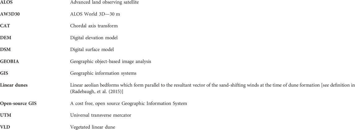
Keywords: geographic object-based image analysis (GEOBIA), open-source geographic information systems (GIS), geomorphic mapping, linear dunes, Kati Thanda (Lake Eyre), Australia
Citation: Fischer LM, Sommer C and Fitzsimmons KE (2023) An open-source GIS approach to understanding dunefield morphologic variability at Kati Thanda (Lake Eyre), Central Australia. Front. Earth Sci. 11:1196244. doi: 10.3389/feart.2023.1196244
Received: 29 March 2023; Accepted: 14 July 2023;
Published: 31 July 2023.
Edited by:
Joel Roskin, Bar-Ilan University, IsraelReviewed by:
Lotem Robins, Bar-Ilan University, IsraelSteven L. Forman, Baylor University, United States
Copyright © 2023 Fischer, Sommer and Fitzsimmons. This is an open-access article distributed under the terms of the Creative Commons Attribution License (CC BY). The use, distribution or reproduction in other forums is permitted, provided the original author(s) and the copyright owner(s) are credited and that the original publication in this journal is cited, in accordance with accepted academic practice. No use, distribution or reproduction is permitted which does not comply with these terms.
*Correspondence: Lorenz M. Fischer, bC5tLmZpc2NoZXJAdC1vbmxpbmUuZGU=