Arctic stratosphere changes in the 21st century in the Earth system model SOCOLv4

1 Introduction

Observed and projected increase in greenhouse gas (GHG) concentrations in the atmosphere leads to a warming in the troposphere and to a cooling in the stratosphere, which affects its circulation and chemical composition, accelerating the return of ozone concentrations to pre-1980 levels (WMO, 2002; Chipperfield et al., 2017; Baldwin et al., 2019). Notwithstanding the measures taken and planned by the majority of countries to reduce GHG emissions in the framework of the Kyoto Protocol and following the Paris Agreement, the increase in GHG concentrations will undoubtedly continue throughout the 21st century.

The cooling of the stratosphere enhances the increase in ozone concentration above 10 hPa, driven by the reduction of halogen loading due to the implementation of the Montreal Protocol and its amendments and adjustments (MPA) due to a slowdown of the temperature-dependent catalytic ozone depletion cycles (Zubov et al., 2013; WMO, 2022). An increase in other GHGs such as methane (CH₄) further promotes the enhancement of the ozone layer in the upper stratosphere via the reaction CH₄+Cl→CH₃+CHCl (Hitchman and Brasseur, 1988). However, the increase in nitrous oxide (N₂O) can intensify ozone loss through catalytical reactions involving NOx (Revell et al., 2012). Possibly, N₂O will be the most important anthropogenic compound contributing to the delay of ozone layer recovery throughout the 21st century (Chipperfield, 2009; Wang, et al., 2014).

While an increase in ozone in the upper stratosphere has already been observed and is likely to continue in the coming decades, the recovery of the ozone layer in the lower stratosphere is less evident. For instance, a statistically robust negative tendency was found for the ozone layer between 146 hPa and 32 hPa on the near-global scale (55°S–55°N) by Ball et al. (2018).

The possible reasons that might contribute to the ozone decline in the lower stratosphere are as follows: a change in the relative strengths of the lower and upper branches of the meridional Brewer–Dobson circulation (BDC) discussed by Butchart et al. (2010) and Keeble et al. (2021); the recent reduction in solar activity (Arsenovic et al., 2018); the influence of halogen-containing very short-lived species and other gases unaccounted for by the MPA (Oram et al., 2017); increased emissions of inorganic iodine (Karagodin-Doyennel et al., 2021); increased aerosol loading (Andersson et al., 2015); unexpected increase in emissions of trichlorofluoromethane (CFC-11) violating the MPA (Fleming et al., 2020); changes in the extratropical tropopause altitude (Bognar et al., 2022). Chipperfield et al. (2018) argued that dynamical processes are the main reason for the decline in lower stratospheric ozone rather than short-lived chlorine species.

Analysis of 20 climate models participating in the CMIP6 project (including four models with interactive chemistry) showed that lower extratropical stratosphere cooling related to GHG emission could contribute to the strengthening of the stratospheric polar vortex, and hence to the ozone depletion in the Arctic stratosphere, especially under the shared socioeconomic pathways 5.8-5 (SSP 5.8-5) of GHG emission growth in the 21st century (von der Gathen et al., 2021). This conclusion was confirmed by analysis of INM-CM5 simulations (Vargin et al., 2022). After the 2050s, dynamical conditions in the Arctic stratosphere in some winters could be favorable for substantial ozone destruction in the late winter and spring despite the expected continuation of the ozone-depleting compound decline due to implementation of the MPA (von der Gathen et al., 2021).

However, analysis of 55 climate model simulations performed in the framework of CMIP6 showed that climate models do not agree on whether the Arctic stratospheric polar vortex will weaken or strengthen during the 21st century (Karpechko et al., 2022). The reason is the large uncertainty in the projected strength of the polar vortex, and the half of this uncertainty by the end of the 21st century is due to climate model deficiencies (Karpechko et al., 2022).

Notwithstanding the expected ODS concentration decline, a possibility of large ozone depletion events in the Arctic even beyond 2060 was shown in 50 of 500 ensemble models of CCM MIROC3.2 simulations (Akiyoshi et al., 2023).

Multiple chemistry-climate modeling (CCM) simulations indicate that the anticipated ozone recovery in late winter will be sensitive not only to the ozone-depleting substance decline due to MPA realization but also to the possible stratospheric polar vortex shift, resulting in negative and positive total column ozone anomaly centers over northern Eurasia and North America, respectively. Therefore, the ozone recovery in late winter could be substantially delayed in some regions of the Northern Hemisphere extratropical regions (Zhang et al., 2018). Arctic sea-ice loss presumably has contributed to a persistent late-winter shift of the polar vortex toward the Eurasian continent over the past 3 decades (Zhang et al., 2016).

According to model calculations, an increase in the GHG concentrations will be accompanied by an acceleration of BDC and the transport of tracers (Garcia and Randel, 2008). Model calculations showed an increase in upward movements in the tropics of approximately 1% per decade in the upper and 2% per decade in the lower stratosphere until the end of the 21st century. As a result, the average age of stratospheric air decreases up to 60 and 30 days per decade in the upper and lower stratosphere, respectively (Oberländer et al., 2013). However, significant differences remain between model estimates, assimilation data used, and observations. For instance, the trend of downward movement strength in extratropical latitudes remains unclear. An analysis of CMIP6 historical simulations confirms the known inconsistency in the sign of BDC trends between observations and models in the middle and upper stratosphere (Abalos et al., 2021).

The present study aims to evaluate stratospheric dynamic changes relevant to Arctic stratospheric ozone from 2015 to 2099 using the Earth system model (ESM) SOCOLv4 (SOlar Climate Ozone Links, version 4, hereinafter referred to as SOCOLv4). The model includes interactive chemistry (Sukhodolov et al., 2021), which is important for simulations of temperature, ozone, and stratosphere–troposphere dynamical coupling in the Arctic stratosphere (Rieder et al., 2019; Haase and Matthes, 2019; Friedel et al., 2022).

2 The SOCOLv4, experiment setup, data description, and analysis methods

The SOCOLv4 is based on the Max Planck Institute for Meteorology (MPIM) Earth system model (ESM) version 1.2 (MPI-ESM1.2) (Mauritsen et al., 2019) that is interactively coupled to the chemical module MEZON (Model for Evaluation of oZONe trends), the size-resolving sulfate aerosol microphysical module AER, the ocean dynamical model MPIOM 1.6.3, and the ocean biogeochemistry model HAMOCC6 (Sukhodolov et al., 2021).

The SOCOLv4 is formulated on the horizontal spectral resolution grid with T63 triangular truncation (approximately 1.9 × 1.9° grid spacing) and 47 vertical levels from the surface to 0.01 hPa (∼80 km) in a sigma pressure coordinate system. The main time step in SOCOLv4 is 15 min, whereas full radiation and chemistry calculations are carried out every 2 h.

We analyze two SOCOLv4 experiments over the period of 2015–2099 driven by moderate (SSP2–4.5) and severe (SSP5–8.5) scenarios (Riahi et al., 2017) of GHG emission evolution. Under the SSP2–4.5 scenario, by the end of the 21st century, the radiative forcing will increase by approximately 4.5 W/m² compared to the pre-industrial climate (before 1750). The concentration of carbon dioxide (CO₂) will increase to ∼600 ppm. Under the SSP5–8.5 scenario, with an increase in radiative forcing by approximately 8.5 W/m², the CO₂ concentration increases four times to 1,135 ppm. The global mean surface temperature is expected to increase by approximately 3°C and 5°C at around 2100 under these scenarios (Zhao et al., 2020).

Each model simulation consists of three ensemble members initialized with slightly changing initial conditions: 0.1% perturbation of the first-month CO₂ concentration. A detailed description of analyzed model experiments is presented by Karagodin-Doyennel et al. (2023).

As the vertical resolution of the SOCOLv4 (based on ECHAM6 with 47 vertical levels) in the atmosphere is insufficient for a reasonable self-generation of the quasi-biennial oscillation (QBO), it was set as three repeating cycles according to Giorgetta et al. (2016).

All climate forcings following the recommendations of CMIP6 (Eyring et al., 2016) are branched to either SSP2-4.5 or SSP5-8.5 scenarios using projected GHG concentrations since 2015. The future solar irradiance projection is provided by HEPPA/SOLARIS as it is also recommended for CMIP6 (Matthes et al., 2017; Eyring et al., 2016).

Polar stratospheric clouds (PSCs) play a critical role in ozone depletion in the late winter and spring. PSCs are composed of supercooled ternary solutions (STS; H₂SO₄–HNO₃–H₂O mixtures), crystalline nitric acid trihydrate (NAT) (PSC type I), and water ice (PSC type II). PSCs provide media for the conversion of inert reservoir species like HCl, HBr, and ClONO₂ to Cl₂, BrCl, and ClNO₂. Later, it transforms into active forms in the presence of solar light (Solomon et al., 1986), leading to ozone depletion induced by catalytic cycles during spring (Molina and Molina, 1987). NAT particles are also responsible for denitrification because gravitational sedimentation can remove reactive nitrogen from the stratosphere, which contributes to ozone depletion by hindering the formation of inactive reservoir species (Salawitch et al., 1993). Therefore, a good representation of PSCs is indispensable for CCM, considering the ozone layer variability and long-term changes and its coupling with atmospheric dynamics.

In SOCOLv4, as in SOCOLv3.1, STS droplets form upon the uptake of gas-phase HNO₃ and H₂O by liquid sulfuric acid aerosols, according to Carslaw et al. (1995).

Analysis of SOCOLv3 PSC representation in comparison with satellite and ground-based observations showed overall good temporal and spatial agreement between modeled and observed PSC occurrence and composition (Steiner et al., 2021). This justifies the following analysis of PSC parameter evolution in the Arctic throughout the 21st century in the simulations of SOCOLv4 with the same PSC scheme as in SOCOLv3.

SOCOLv4 calculations over recent decades have shown marginally significant negative ozone changes in the low-latitude lower stratosphere, which agrees in general with the negative tendencies extracted from the satellite data (Karagodin-Doyennel et al., 2022).

The future evolution of the ozone layer throughout the 21st century under moderate (SSP2-4.5) and severe (SSP5-8.5) GHG emission scenarios was also investigated using SOCOLv4 simulations (Karagodin-Doyennel et al., 2023). The results suggest a very likely ozone increase in the mesosphere, upper and middle stratosphere, and in the lower stratosphere at high latitudes. Under SSP5–8.5, the ozone increase in the stratosphere is higher because of stronger cooling induced by GHG emissions, which slows the catalytic ozone destruction cycles. In contrast, in the tropical lower stratosphere, ozone concentrations were found to decrease in both experiments due to stronger upwelling and increase over the middle and high latitudes of both hemispheres due to the intensification of meridional transport, which is stronger in SSP5-8.5.

In the present study, we use monthly mean output data of simulations with three ensemble methods as in Karagodin-Doyennel et al. (2023) and consider temperature, zonal wind, zonal heat flux, amplitude of planetary waves, surface area density (SAD) of solid nitric acid trihydrate (NAT) particles, and liquid STS droplets of the PSCs type I under the moderate and severe GHG emission scenarios. Furthermore, the changes in HNO₃, H₂O, and O₃ concentrations throughout the 21st century were investigated.

To characterize the interannual variability of the Arctic stratosphere, the volume of low stratospheric air with temperatures below the polar stratospheric cloud formation threshold (hereafter Vpsc) and the stratospheric polar vortex volume (Vvortex) were calculated according to Lawrence et al. (2018) using SOCOLv4 model data, similar to the INM CM5 simulation analysis for the modern and future climate (Vargin et al., 2020; Vargin et al., 2022).

First, potential vorticity (PV) was calculated on isobaric surfaces using monthly 3D model data on temperature, horizontal wind speed, and geopotential height. Then, the PV and temperature values ​​were interpolated to the potential temperature levels (isentropic levels), at which the maximum PV gradient from the equivalent latitude was calculated and the corresponding PV value was denoted as the polar vortex boundary. Then, these values ​​were averaged over January–March and used to determine the climatic boundary and the area of the polar vortex (Lawrence et al., 2018).

Furthermore, the temperature threshold for PSC NAT formation (Tnat) was calculated based on the pressure levels using average vertical profiles of H₂O and NHO₃ concentrations in the 60°N−90°N polar cap during the winter season (Hanson and Mauersberger, 1988). Then, Tnat is interpolated on the isentropic levels and used to estimate ​​the area where PSC NAT formation is possible. At each isentropic level, the grid cell was related to the PSC region if it was inside the boundary of the polar vortex and the temperature in the cell was below the critical value.

The Vpsc and the Vvortex were calculated for the range of the lower stratosphere heights from 390 K to 590 K (∼120 hPa–∼ 30 hPa) over the known area at each level and thickness of the isentropic layers by summing the areas with appropriate weights.

To analyze changes in wave activity propagation into the extratropical boreal stratosphere, the following parameters were estimated using monthly mean SOCOLv4 output data: amplitudes of planetary waves with zonal numbers 1–3, zonal mean meridional heat flux, two-dimensional Eliassen–Palm (EP) flux, and three-dimensional Plumb flux vectors characterizing the propagation of wave activity flows (Plumb, 1985) (see Supplementary Material S1). The 3D planetary wave activity flux by Plumb in comparison with conventional 2D EP flux can provide more information on stratosphere–troposphere dynamical interactions and wave activity propagation (e.g., Gečaitė, 2021; Wei et al., 2021). In addition, the divergence of EP fluxes characterizing an influence of wave activity propagation on the zonal mean circulation (acceleration/deceleration) was estimated.

For further diagnostics of dynamical processes, the residual mean meridional circulation (RMC) was calculated based on the conventional transformed Eulerian mean approach (TEM, Andrews and McIntyre, 1976) (Supplement Material S2). RMC is a superposition of eddy-induced and advective zonal mean flows. Calculation of meridional (V*) and vertical (W*) RMC components is widely used to analyze the interaction between planetary waves and the mean flow and gives the ability to estimate the meridional transport of long-living tracers in the atmosphere. Basically, RMC is that part of the mean flow which remains after partial compensation of the advective processes by the wave-induced eddy mass, momentum, and heat fluxes (Shepherd, 2007). A description of methods used to calculate the RMC can be found in Koval et al. (2021).

The significance of the trends revealed in the model simulations was estimated according to Student’s t-test on a significance level of 95%.

3 Results

We focus our analysis on temperature and global circulation changes throughout the 21st century in March when the largest ozone loss is observed in the Arctic lower stratosphere in the winters with the cold and persistent stratospheric polar vortex. To analyze possible changes in stratospheric large-scale dynamical processes and stratospheric polar vortex parameters, the differences in the ensemble mean zonal mean temperature, zonal mean wind, RMC, zonal mean meridional heat flux, amplitudes of wavenumber from 1 to 3, 2D Eliassen–Palm, and 3D Plumb fluxes characterizing planetary wave (PW) activity propagation between the 20-year time periods in the end and at the beginning of the 21st century (2080–2099 and 2015–2034) are considered.

3.1 Temperature and zonal wind changes

First, the changes in zonal mean temperature, zonal wind, and RMC were analyzed. Shaded areas in Figures 1A, D illustrate latitude–height distributions of zonal mean temperature and zonal wind simulated with SOCOLv4 in March averaged over 2015–2034. Arrows in Figure 1A show components of RMC, and gray contours in Figure 1D illustrate EP flux divergence. Differences in respective values between 2080–2099 and 2015–2034 are presented in the center (SSP2–4.5) and right (SSP5–8.5) panels of Figure 1. Under SSP2–4.5, the cooling in March by the end of the 21st century ranges from ∼1 K in the lower stratosphere to ∼3 K in the upper stratosphere and mesosphere (Figure 1B). As expected, application of SSP5–8.5 leads to a stronger decrease in temperature from ∼1 K in the lower stratosphere to ∼10 K in the upper stratosphere (Figure 1C). Under SSP2–-4.5, temperature changes are stronger in the Arctic stratosphere: up to ∼4 K, while under SSP5–-8.5, the temperature changes in the Arctic stratosphere are smaller relative to those at middle latitudes. In general, expected cooling of the stratosphere and mesosphere and warming of the troposphere are observed (Figures 1B, C) that agrees with previous results ( Steiner et al., 2021; Butchart, 2022). In addition to the temperature changes, a general increase in RMC components is obtained (RMC increments in Figures 1B, C that are mainly co-directed to the RMC components shown in Figure 1A). However, there are some exceptions that are described further. The strongest increments are seen in the upper stratosphere and mesosphere and in the upper troposphere. Enhancement of the RMC is much stronger under the SSP5–-8.5, at which wind amplification can reach up to 20% (Figure 1C). Acceleration of the RMC due to increasing GHG emissions was repeatedly predicted in most CCMs ( Butchart et al., 2010). Here, we are talking about the study of the advective component of the RMC, while the wave-induced eddy component is directly associated with the activity of PWs, the structure of which is considered in the following section. In particular, our calculations show that weakening of the eddy component of RMC causes a weakening of the downward RMC branch in the Arctic stratosphere (1 hPa–10 hPa) as shown in Figure 1B, which, in turn, is likely to be the main cause of cooling in this area by the end of the 21st century under the SSP2–-4.5. Under the SSP5–-8.5, the weakening of wave activity is observed in another area: in the lower stratosphere (50 hPa–100 hPa), at middle latitudes. There is also a weakening of the RMC in this area. Strengthening of the RMC by the end of the 21st century, especially under SSP5–8.5, significantly affects the composition of the middle atmosphere; in particular, the age of air decreases (e.g., Waugh, 2009).

FIGURE 1

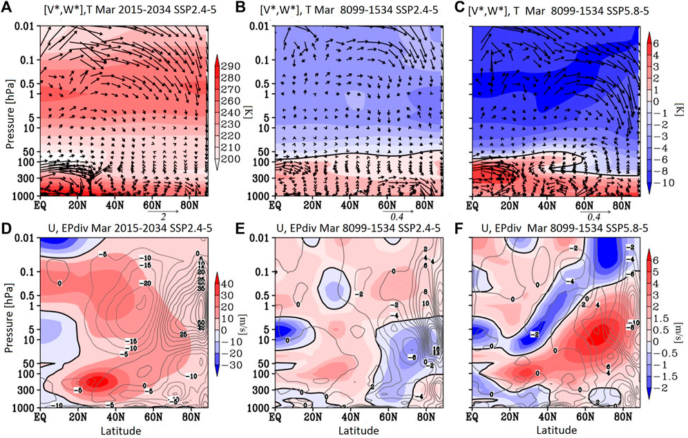
FIGURE 1. Latitude–height distributions of the meridional V* and vertical W* components of the RMC (m/s, vertical component multiplied by 200) (vectors) and zonal mean temperature (K) (shaded) in March 2015–2034 (A) and respective changes between the periods 2080–2099 and 2015–2034 under SSP2-4.5 (B) and SSP5-8.5 (C). Zonal mean zonal wind (m/s) (shaded) and EP flux divergence (m²/s²/day) (contours) for March 2015–2034 (D); respective changes between the periods 2080–2099 and 2015–2034 under SSP2-4.5 (E) and SSP5-8.5 (F).

Stratospheric temperature and RMC changes lead to enhancement of the zonal mean zonal wind of the high latitudinal lower–middle stratosphere to 1–2 m/s under the moderate GHG emission scenario and up to 6 m/s under the severe GHG emission scenario (Figures 1E, F). For example, the enhancement of the meridional, northward component of the RMC in the stratosphere under both GHG scenarios through the Coriolis force corresponds to the eastward acceleration of the zonal wind. Under the moderate GHG emission scenario, however, the PW-induced weakening of the eddy component of the RMC in the Arctic stratosphere can also cause deceleration of the zonal wind between 5 hPa and 100 hPa in Figure 1E.

However, in addition to GHG emission growth, the changes in PW activity (that, in turn, could be caused by zonal circulation changes related to GHG emission growth) might also contribute to stratospheric dynamic changes. To analyze this, we calculated the changes in the divergence of the EP flux. These increments are shown with gray contours in Figures 1E, F. The main reason for the weakening of the zonal wind below 3–5 hPa under the moderate GHG emission scenario is the negative increment of the EP flux divergence, which corresponds to the energy transfer from the mean flow to the PWs (Figure 1E). A similar process is observed in the stratosphere and mesosphere of middle latitudes under the severe GHG scenario (Figure 1F). In this case, in the polar region, on the contrary, there is a sink of wave energy in favor of the mean flow (a positive increment in the EP flux divergence). This sink contributes to the acceleration of the zonal wind. In both scenarios, the strengthening of subtropical jets in the lower stratosphere (∼2 m/s and ∼4 m/s for the moderate and severe GHG emission scenario, respectively) is explained by the strengthening of temperature meridional gradients according to the thermal wind theory. In addition, wave energy transport toward the mean flow (expressed in the EP flux divergence) contributes to the strengthening of the subtropical jet.

3.2 Heat flux and planetary wave activity propagation changes

It is known that the upward propagation of planetary wave activity can be characterized by zonal mean meridional heat flux $\overline{v’T’}$ (hereafter heat flux HF) averaged over high latitudes, where v’ and T’ are deviations of meridional wind and temperature, respectively, from zonal mean. Heat flux in the lower stratosphere in January–February correlates with the lower polar stratosphere temperature in March (Newman et al., 2001) when the largest ozone layer destruction occurs. This correlation was employed particularly for validation of CCM simulations (Austin et al., 2003).

In the analyzed SOCOLv4 simulations, the correlation coefficient between heat flux in the lower stratosphere in January–February and the lower polar stratosphere temperature in March in both scenarios is ∼0.5 (Figures 2A,B).

FIGURE 2

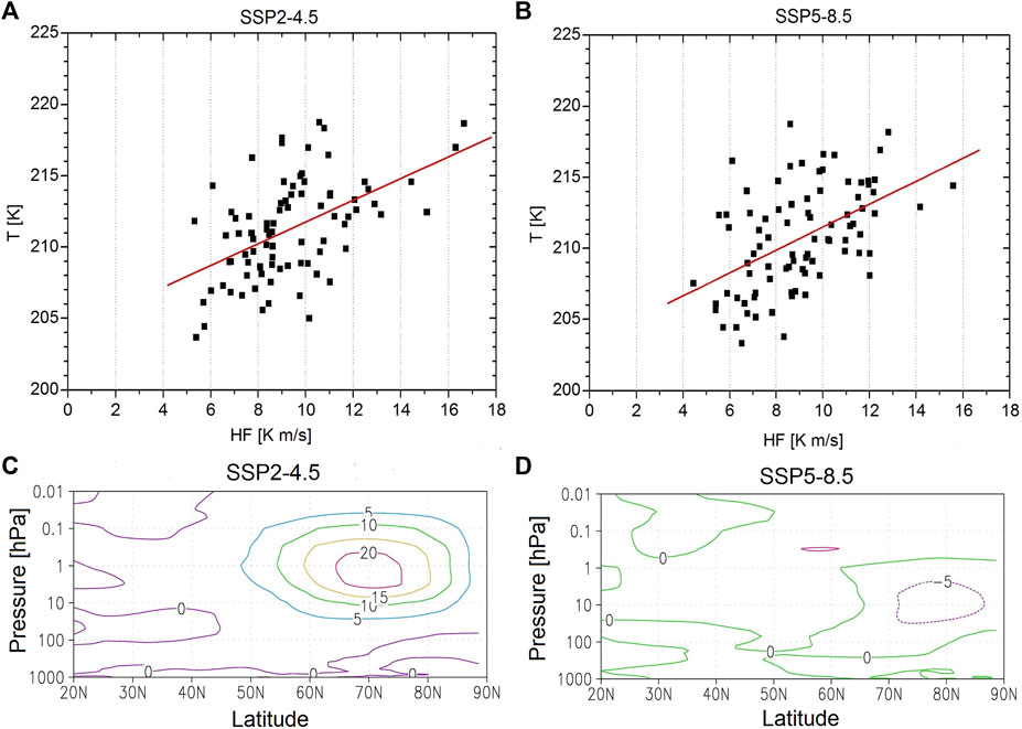
FIGURE 2. Scatter diagrams of heat flux HF (K m/s) over 45°–75 N at pressure level 100 hPa averaged over January–February and temperature over 70°N–90°N at 70 hPa in March of the ensemble mean under SSP2-4.5 (A) and SSP5-8.5 (B) scenarios. Heat flux (K m/s) differences of the ensemble mean in January–February between the periods 2080–2099 and 2015–2034 under SSP2-4.5 (C) and SSP5-8.5 (D) scenarios.

Furthermore, the changes of heat flux in January–February throughout the 21st century were studied. In the late period of the 21st century, the strengthening of heat flux with a maximum of up to 20 K m/s (∼25%) in the upper stratosphere close to 70°N is obtained in the moderate GHG emission scenario (Figure 2C). Under In the severe GHG emission scenario, we observe a slight increase in heat flux over 50°N–60°N with the maximum of up to 5 K m/s in the upper stratosphere and a decrease with the comparable values over the high latitudes (Figure 2D).

The similar heat flux difference in both scenarios is found if the 30-year periods of 2070–2099 and 2015–2044 are compared (Supplementary Figures S3).

We also analyze the changes dominated by the extratropical stratosphere planetary waves with wavenumbers from 1 to 3 in January–February. Amplitudes of these wavenumbers averaged over 2015–2034 are presented in Figure 3A, B. While the maximum amplitude of wavenumber 1 up to 600 gpm is found in the middle and upper stratosphere over high latitudes, the maximum amplitude of wavenumber 2 is approximately 150 gpm and observed in the lower and middle stratosphere.

FIGURE 3

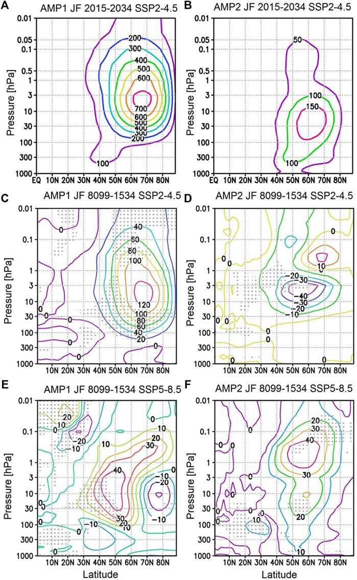
FIGURE 3. Amplitude of wavenumbers 1 and 2 (gpm) averaged over January–February in the period of 2015–2034 under SSP2.4–5 (A, B), the difference in amplitude of wavenumbers 1 (C, E) and 2 (D, F) in January–February between the periods 2080–2099 and 2015–2034 under SSP2.4–5 (C, D) and SSP5.8–5 (E, F) scenarios. The regions with significance at the 95% level for positive or negative changes are marked by gray dots.

In the moderate GHG emission scenario, the amplitude of wavenumber 1 increases up to 120 gpm in the middle stratosphere nearby 70°N (Figure 3C). The wavenumber 2 amplitude changes are characterized by slight decrease (Figure 3D). In contrast to the moderate GHG emission scenario, the wavenumber 1 amplitude does not show an increase in the severe GHG emission scenario (Figure 3E). Strengthening of wavenumber 2 amplitude occurs only in the upper extratropical stratosphere.

The amplitude of wavenumber 3 is significantly weaker than that of wavenumbers 1 and 2 (Supplementary Figures S4A). In the moderate GHG emission scenario, the amplitude of wavenumber 3 decreased in the lower stratosphere over the middle–high latitudes up to −15 gpm and slightly increased up to 5 gpm in the upper stratosphere over the latitudinal belt 50°N–60°N (Supplementary Figures S4B), while in the severe GHG emission scenario, the amplitude of wavenumber 3 increased in the lower stratosphere up to 10 gpm and decreased in the upper stratosphere up to −15 gpm over the latitudinal belt 40°N–70°N (Supplementary Figures S4C).

Furthermore, a statistical significance of wave number 1 and 2 amplitude differences between the periods 2080–2099 and 2015–2034 under SSP2–4.5 and SSP5–8.5 scenarios was estimated. To estimate the significance of wave amplitude differences of the data, the two-sample Welch’s unequal variances t-test was used (Wilks 2006).

Under SSP2-4.5 scenario the regions with significance at the 95% level for wavenumber 1 differences are observed over middle–high latitudes, whereas under SSP5–8.5, such regions are less pronounced and limited by the 30°N–50°N latitudinal belt in the lower–middle stratosphere (Figure 3C, E). For wavenumber 2 differences, the regions with significance at the 95% level are limited by middle stratosphere over middle latitudes under SSP2–4.5 scenario. Under SSP5–8.5 scenario, such regions are fewer and observed only over high latitudes in the upper and lower stratosphere (Figures 3D, F).

Furthermore, the changes in planetary wave activity propagation were studied using calculated 2D Eliassen–Palm fluxes. Under the SSP2-4.5 scenario, we obtained an increasing upward wave activity propagation over the latitudinal belt 50°N–70°N in January–February in the period of 2080–2099 in comparison with 2015–2034 in the middle and upper stratosphere (Figure 4A). It is in agreement with zonal mean heat flux changes (Figure 2C). Under the SSP5–8.5 scenario, a strengthening of upward and equatorward wave activity propagation is limited by the latitudinal belt 30°N−50°N. At higher latitudes, a weakening of upward wave activity propagation is observed (Figure 4B), which is also in agreement with zonal mean heat flux changes (Figure 2D).

FIGURE 4

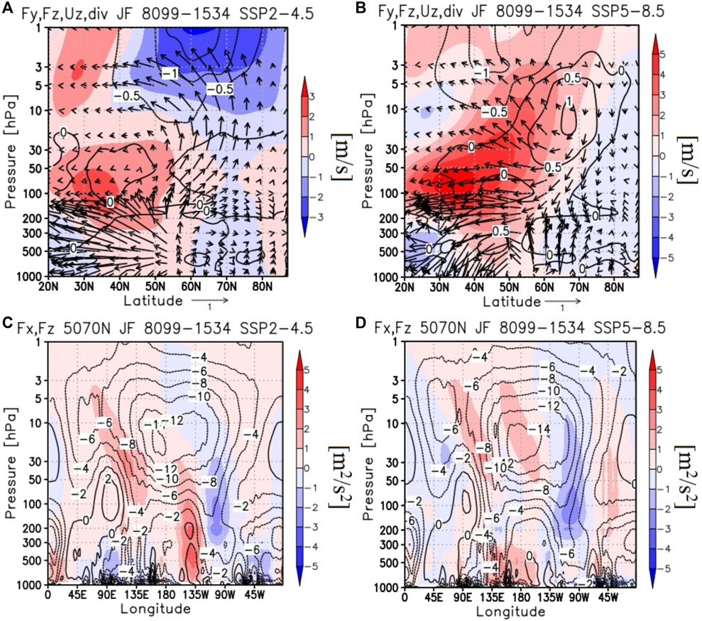
FIGURE 4. Latitude–height cross-section of meridional F_y (m²/s²), vertical component F_z (m²/s².10^-2) of EP fluxes (vectors), EP divergence (m/s/day) (contours), and zonal mean zonal wind (m/s) (shaded) increments between the periods 2080–2099 and 2015–2034 under SSP2–4.5 (A) and SSP5–8.5 scenario (B). Altitude–longitude cross-section of F_x (m²/s²) (contours) and F_z component (m²/s² 10^-2) (shaded) of Plumb flux increment in January–February averaged over 50°N–70°N under SSP2–4.5 (C) and SSP5–8.5 scenarios (D).

To investigate the impact of wave activity propagation on the zonal circulation, the EP divergence is shown (Figure 4). From the zonal mean point of view, the deposition of easterly angular momentum in the stratosphere due to the convergence of planetary wave activity fluxes caused strong deceleration of the zonal mean zonal wind and the sudden stratospheric warming (SSW), in accordance with Matsuno’s theory (Matsuno, 1971).

Under SSP2–4.5 scenario, a negative divergence in the middle and upper stratosphere over the high northern latitudes (∼40°N–70°N) indicates additional wave forcing from the troposphere and lower stratosphere in the late 21st century (2080–2099), which decelerates the westerly flow (Figure 4A). The area of negative divergence increment corresponds to the area of weakening of zonal wind, which is increased with height: on ∼1 m/s in the middle stratosphere and on ∼3 m/s in the upper stratosphere. Upward and poleward increments of wave activity fluxes in the extratropical stratosphere indicate stronger upward and poleward wave activity propagation in the period of 2080–2099 than in the period 2015–2034.

Under the SSP5–8.5 scenario, a positive divergence increment over the high northern latitudes with the maximum nearby 10 hPa and poleward tilt in January–February indicates that additional wave forcing contributes to the acceleration of westerly flow (Figure 4B). This area of positive EP divergence increment corresponds to the area of strengthening of zonal wind by approximately 2–4 m/s and also exhibits a poleward tilt. Downward and equatorward increments of wave activity fluxes in the lower and middle extratropical stratosphere indicate lesser upward and poleward wave activity propagation in the period of 2080–2099 than in the period 2015–2034.

Analysis of changes in the longitudinal structure of wave activity propagation averaged over 50°N–70°N between late and early 20-year periods of the 21st century under both scenarios shows a weakening of eastward wave activity propagation (F_x—longitudinal component of Plumb fluxes) which is observed in the entire stratosphere, with the maximum in the middle stratosphere nearby 30 hPa−10 hPa and at the dateline (Figures 4C, D). The exceptions are significantly less two areas of weak F_x strengthening in the middle stratosphere over the northeastern part of the Atlantic Ocean (45° W– 0°) and in the lower stratosphere nearby 90°E. Interestingly, the weakening of F_x over northern Eurasia throughout the 21st century is comparable under both scenarios. The weakening of F_x that dominated in the extratropical stratosphere is also observed at the similar altitude–longitude cross-section of the mean latitude band 40°N–60°N (Supplementary Figures S5A, B). A potential explanation of dominant F_x weakening in the extratropical stratosphere over northern Eurasia lies in the limitation of this area from west by the area of the downward propagation strengthening (Fz component) over the northern part of North America.

Under the SSP2–4.5 scenario, a vertical propagation of wave activity changes is revealed in the three dominated areas: two with strengthening and one with weakening. The first two areas with strengthening lasted from the troposphere to the middle stratosphere over a rather thin longitudinal belt centered nearby 130°W and the second one in the lower and middle stratosphere slightly tilted westward over the longitudinal belt ∼90°E−130°E. Strengthening of downward wave activity propagation is expected from the upper stratosphere to the upper troposphere over the longitudinal belt 150°W– 90°W.

Under the SSP5–8.5 scenario, the strengthening of upward wave activity propagation is observed in three areas: two slightly tilted westward over 90°E−120°E, 180°W–160°W, and 50°W–40°W, while strengthening of downward propagation is expected over 140°W–90°W.

The changes in vertical wave activity propagation using Plumb vertical component Fz in January–February are also illustrated by stereographical polar projections on the pressure levels of 100 hPa (Supplementary Figures S5C-E). A spatial structure of Fz in the extratropical lower stratosphere averaged over the period of 2015–2034 is characterized by upward wave activity propagation over northern Eurasia with the maximum over south of Eastern Siberia–Northern China and north of Pacific Ocean and downward propagation over the north of Northern America with approximately two times weaker magnitude (Supplementary Figures S4C). The major feature of Fz changes in the extratropical lower stratosphere throughout the 21st century is the strengthening of downward propagation over the north of Northern America in 1.5–2 times (Supplementary Figures S4D, E).

3.3 Stratospheric polar vortex shift toward northern Eurasia

A shift of the polar vortex toward northern Eurasia throughout the 21st century was revealed in the last 3 decades in observational data and model simulations (Zhang et al., 2016; Karpechko et al., 2022). It was suggested that this shift was mainly caused by Arctic sea-ice loss and could lead to negative total ozone anomalies over Northern Eurasia and positive anomalies over the northern part of North America (Zhang et al., 2018). The other possible cause of expected asymmetry of the Arctic stratospheric polar vortex throughout the 21st century is a warming in the eastern equatorial Pacific Ocean that leads to eastward-shifted teleconnection with a deepened Aleutian Low, which strengthens the polar vortex over Eurasia and weakens over North America by enhancing the vertical wave propagation into the stratosphere (Matsumura et al., 2021).

Under both scenarios, a shift of the stratospheric polar vortex toward the east of northern Eurasia in the lower stratosphere in January–February was revealed in SOCOLv4 simulations. This shift is tilted westward with the height and maximized nearby 160°E in the middle stratosphere and nearby 90°E in the upper stratosphere (Figures 5A, B). The shift of the polar vortex toward the east of northern Eurasia in the lower stratosphere in January–February in simulations under both scenarios can be illustrated as a geopotential height difference between the 2080–2099 and 2015–2034 time periods. As an example, this difference at pressure level 30 hPa is plotted on Figure 5C, D. In the upper stratosphere, this difference increases (Supplementary Figures S6A-D). A similar shift of the stratospheric polar vortex is also observed in March (Supplementary Figures S6E-H).

FIGURE 5

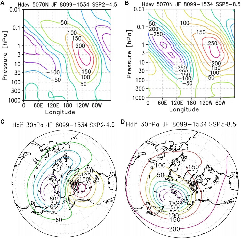
FIGURE 5. Longitude–height cross-section of January–February eddy geopotential height (gpm) averaged across 50°N−70°N latitude difference between 2080–2099 and 2015–2034 time periods under the SSP2–4.5 (A) and SSP5–8.5 scenarios (B). Geopotential height of January– February mean at the pressure level 30 hPa differences between the same time periods under the SSP2–4.5 and SSP5–8.5 scenarios (C, D).

3.4 Arctic stratospheric polar vortex changes

We have studied some polar vortex characteristics which include polar vortex volume (Vvortex), air volume with temperatures below the PSC formation threshold (Vpsc), and maximal gradient of scaled potential vorticity (MPVGs). These parameters describe the volume of air inside the stratospheric polar vortex, air volume inside the polar vortex, which temperature is below critical temperature of PSC NAT formation, and strength of dynamical barrier between vortex air and outside.

The critical temperature of PSC NAT formation depends on the concentrations of HNO₃ and H₂O (Hansen and Mauersberger, 1988); therefore, first, we have examined the evolution of profiles of these chemical components.

The average concentration of HNO₃ is slightly increased only nearby its maximum in the Arctic lower stratosphere, throughout the 21st century. The concentration of water vapor is increasing up to 0.5 ppm in the stratosphere under the SSP2–4.5 scenario (Figures 6A, B). Underthe SSP5–8.5 scenario, the average concentration of HNO₃ is stable, while the concentration of water vapor is increasing up to 1–1.5 ppm in the stratosphere during the late 21st century (Figures 6C, D). The critical temperature of PSC NAT formation (Tnat) is calculated using respective concentrations of H₂O and HNO₃. It is also increasing up to 0.5–1.1 K under the SSP5–8.5 scenario (Figure 6E), while under the SSP2–4.5 scenario, it is increasing in the lower stratosphere up to 0.5 K and decreases in the middle stratosphere up to 0.2 K.

FIGURE 6

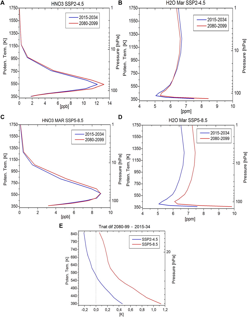
FIGURE 6. Vertical profiles of the mixing ratio of H₂O and HNO₃ of 2015–2034 (blue curve) and 2080–2099 (red) and 60°N–90°N for the ensemble mean of the SSP2–4.5 (A, B) and SSP5–8.5 (C, D) scenarios. Difference in the critical temperature of PSC NAT formation Tnat averaged over and 60°N–90°N and between the periods 2080–2099 and 2015–2034 for the ensemble mean at isentropic and pressure levels of the SSP2–4.5 and SSP5–8.5 scenarios (E).

As shown in additional calculations (not presented), these changes in Tnat profiles only slightly influence the PSC volume average values, and they are not significant for the trend estimates.

An increase in the Vpsc in the Arctic stratosphere by the end of the 21st century is observed in March for all model runs as well as for the ensemble mean. The relative Vpsc (absolute Vpsc divided by Vvortex), which is related to the PSC formation potential proposed in Tilmes et al. (2006), is temporally correlated with Vpsc (Figures 7A, B). The trends of relative and absolute Vpsc in March during the 21st century are significant under the SSP5–8.5 scenario (Figure 7B, C). Meanwhile, the trends of the stratospheric polar vortex volume (Vvortex) are non-significant under both the scenarios (Figures 7E, F). The maximum value of the Vpsc in March for the entire analyzed period in the moderate GHG emission scenario is ∼69 million km³ and ∼62 million km³ in the severe GHG emission scenario. For comparison, according to the MERRA-2 reanalysis (Gelaro et al., 2017), the Vpsc in March 2011 and 2020, when the ozone depletion in the Arctic stratosphere was the greatest overall period of observations, reached ∼29.3 and ∼37.6 million km³, respectively. The maximum values of the relative Vpsc are observed at the end of the 21st century, and they are 0.16 ·10⁻² and 0.14 ·10⁻² for the moderate and severe GHG emission scenarios, respectively.

FIGURE 7

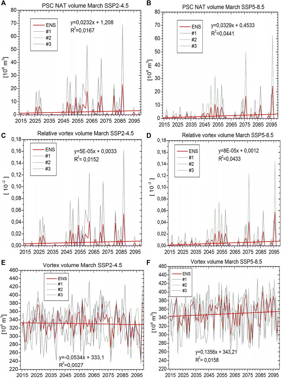
FIGURE 7. Ensemble mean Arctic stratospheric polar vortex characteristics in March from 2015 to 2099: absolute Vpsc (A, B), relative Vpsc (C, D), and the absolute volume of stratospheric polar vortex Vvortex (E, F) under SSP2–4.5 (left) and SSP5-8.5 scenarios (right). Red straight lines correspond to a linear trend.

Nevertheless, total ozone in the Arctic is expected to increase due to smaller ozone loss, which in turn will be caused by ongoing ozone-depleting substances (ODS) decline. Presumably, the latter process will surpass the expected PSC volume increase in the Arctic stratosphere in the late winter throughout the 21st century.

Table 1 presents the climatological values of absolute Vpsc, relative Vpsc, and Vvortex at the beginning and at the end of the 21st century. One could conclude that on average, absolute and relative Vpsc values are increasing by ∼160% and ∼320% at the moderate and severe GHG emission scenarios by the end of the 21st century, respectively. In addition, no significant changes in climatological values of Vvortex were revealed. These conclusions agree with results obtained using the CMIP6 future climate model simulations (von der Gathen et al., 2021; Vargin et al., 2022).

TABLE 1

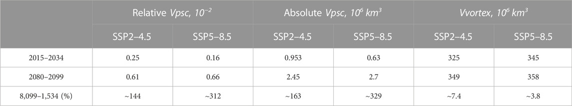
TABLE 1. Ensemble mean of relative Vpsc, absolute Vpsc, and vortex volume Vvortex in March and their differences between the periods of 2080–2099 and 2015–2034 under SSP2–4.5 and SSP5–8.5 scenarios.

The difference in behavior of the Vvortex and Vpsc with time could be explained if we suggest that the PV gradient is increasing to the end of the 21st century, but the position of this maximum is not changing with time significantly. Hence, the polar vortex area (and volume in the lower stratosphere) also is not changing. However, at the same time, air temperature inside the vortex is decreasing, and it may lead to Vpsc growth with time.

The isolation of the stratospheric polar vortex depends on the meridional gradient of the wind speed. Therefore, the maximum gradient of the scaled potential vorticity (MPVG), which assesses the strength of the vortex edge (Lawrence et al., 2015), through winter season from November to April was calculated using ensemble mean output data according to Lawrence et al. (2018). Analysis of its evolution shows that the maximum increase in MPVGs is observed nearby isentropic level 550 K (∼30 hPa/∼23 km) at the end of the 21st century in January–February up to 0.8–1.2 10⁻⁶ s^-1 deg^-1/1.2–1.8 10⁻⁶ s^-1 deg^-1 (∼15%–20%) in the moderate GHG emission scenario and in December–February in the severe GHG emission scenario, respectively (Figure 8A, B). The largest MPVG increase in both scenarios is observed slightly below its maximum at isentropic level 600 K (Supplementary Figures S7). The similar strengthening of the MPVGs was obtained by analysis of the INM CM5 simulations (Vargin et al., 2022).

FIGURE 8

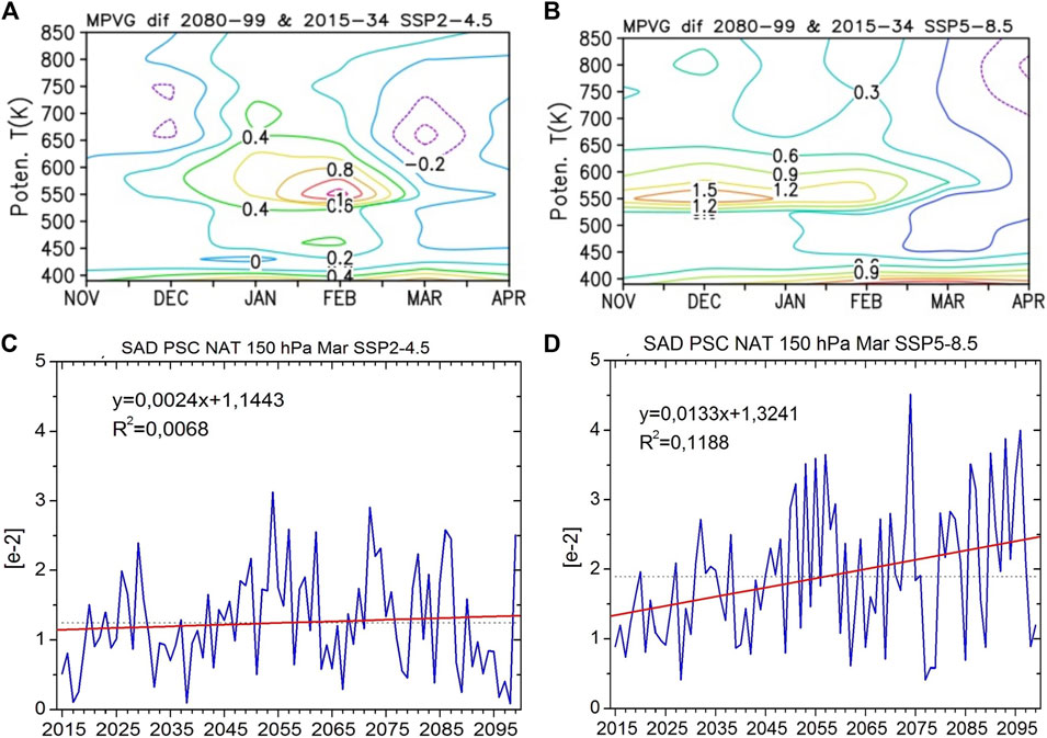
FIGURE 8. Altitude–time diagram of the maximal gradient of scaled potential vorticity ensemble mean (10⁻⁶ s^-1 deg^-1) difference between 2080–2099 and 2015–2034 under SSP2–4.5 (A) and SSP5–8.5 scenarios (B). SAD PSC NAT 60N–90N mean on the pressure level 150 hPa in March from 2015 to 2099 under SSP2–4.5 (C) and SSP5–8.5 scenarios (D).

It is known that the strengthening of the MPVG corresponds to a decrease in effective diffusivity at the polar vortex boundary and to an increase in its isolation (Kostrykin, Schmitz, 2006). Hence, the cooling of the Arctic stratosphere that leads to the increase in the Vpsc NAT and the polar vortex isolation throughout the 21st century revealed in SOCOLv4 simulations indicate its possible strengthening in the lower stratosphere.

To check the consistency of our calculated estimates of PSC NAT with its parameters simulated by SOCOLv4, a long-term variability of surface area density (SAD) of PSC NAT in the lower Arctic stratosphere throughout the 21st century was analyzed. The results show that the respective positive trend of SAD PSC NAT averaged over the latitudinal belt 60°N–90°N on the pressure level 150 hPa in March under the SSP2–4.5 scenario is non-significant but significant under the SSP5–8.5 scenario (Figure 8C, D), which is consistent with trend estimates of calculated Vpsc NAT (Figure 7B).

It is interesting to note that the obtained values of MPVGs are approximately two times smaller than climatological values of MPVGs shown by Lawrence et al. (2018). The plausible reason for this is that our analysis is applied to the monthly mean output data. This may lead to smoothing of the wind meridional gradients in comparison with analysis of the daily mean data.

3.5 Stratospheric water vapor and nitric acid changes

Lower stratospheric water vapor (SWV) is one the most important GHG in the Earth’s atmosphere and drivers of global climate change. Similar to ozone, the past and future changes in SWV have significant impacts on global and regional climate ( Solomon et al., 2010; Dessler et al., 2013; Keeble et al., 2021).

SWV concentrations in the stratosphere are determined predominantly through the dehydration of air masses as they pass through the tropical tropopause cold point and in situ production from CH₄ oxidation (e.g., Keeble et al., 2021). Direct injections by convective overshooting or volcanic eruptions are also sources of SWV.

Increasing SWV influences stratospheric ozone through radiative effects and heterogeneous or HOx-related gas-phase chemistry (Tian et al., 2009). Their CCM simulations showed that the combined chemical and radiative effects of increasing SWV may lead to additional cooling in the tropics and middle latitudes but less cooling in the polar stratosphere and tends to accelerate ozone recovery in the northern high latitudes and slightly delay in the southern high latitudes.

Climate models predict an increase in SWV concentrations under increased CO₂ concentration (Gettelman et al., 2010; Banerjee et al., 2019). This increase over the course of the 21st century occurs due to climate warming compensated in part by the effects of a strengthening BDC (Dessler et al., 2013; Smalley et al., 2017), with additional impacts from future CH₄ emissions (Eyring et al., 2010; Gettelman et al., 2010). A mean increase in 0.5–1 ppmv per century in SWV concentrations was revealed in the models participating in the Chemistry-Climate Model Validation (CCMVal) intercomparison project, although agreement between models on the absolute increase is poor (Eyring et al., 2010).

SWV ensemble mean concentration changes in the Arctic lower stratosphere in March throughout the 21st century in the SOCOLv4 simulations are characterized by a positive significant trend under both scenarios (Figures 9A,NB). Under the SSP5–8.5 scenario, a more pronounced SWV positive trend could be explained by stronger tropospheric water vapor influx into the stratosphere and by enhanced production from CH₄ oxidation.

FIGURE 9

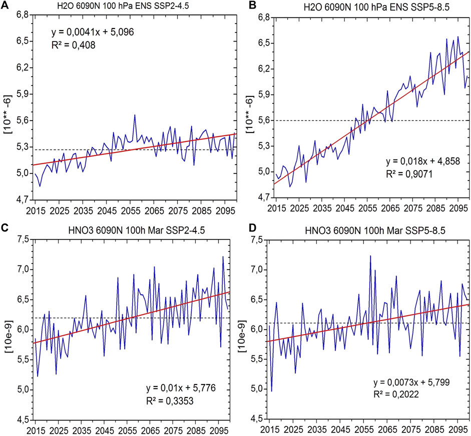
FIGURE 9. Ensemble mean mixing ratio of SWV averaged over 60°N–90°N at the pressure level 100 hPa in March from 2015 to 2099 under the SSP2.4–5 (A) and the SSP5.8–5 (B) scenarios. Ensemble mean mixing ratio of HNO₃ at 100 hPa averaged over 60°N–90°N in March from 2015 to 2099 for the SSP2–4.5 (C) and the SSP5–8.5 (D) scenarios. Red straight and black dashed lines correspond to the linear trend and time mean values, respectively.

HNO₃ is an important chemical constituent in the stratosphere and one of the most abundant species of the NO_y family (NO_y=HNO₃, NO₂, NO, N₂O₅, ClONO₂ , . . .). Below 10 hPa (∼30 km), it is a major reservoir of active odd nitrogen (NOx=NO+NO₂) which is responsible for the main catalytic ozone loss cycle in the middle stratosphere (Urban et al., 2009).

HNO₃ plays an important role in two main processes related to ozone depletion in the polar lower stratosphere. First, heterogeneous chemical processes involving NAT PSC particles, formed from HNO₃, lead to the activation of chlorine from its reservoir gases inside the polar vortex in winter and to ozone loss when sunlight returns after polar night in late winter and spring. Second, denitrification, the irreversible removal of NO_y by sedimentation of HNO₃ containing PSC particles, delays chlorine deactivation through reformation of the chlorine reservoir ClONO₂ during spring and may, therefore, lead to prolonged ozone loss (e.g. Tabazadeh et al., 2001).

HNO₃ ensemble mean changes in the Arctic lower stratosphere in March throughout the 21st century in the SOCOLv4 simulations are characterized by a positive significant trend under both scenarios (Figures 9C,D).

3.6 Sulfur-containing liquid droplets of PSC1

The future state of the ozone layer in the Arctic stratosphere strongly depends on the concentration and composition of the sulfur-containing liquid droplets (Wegner et al., 2012). The supercooled liquid sulfur ternary solution particles (STS, H₂SO₄–H₂O–HNO₃) appear and dominate heterogeneous chlorine activation only if the temperature drops below approximately 192 K. Therefore, the stratospheric sulfuric acid aerosols (SSA, H₂SO₄–H₂O) are mostly responsible for the heterogeneous halogen activation in the relatively warm northern polar vortex area and rare events of ice containing PSC type 2 formation.

The pressure–latitude cross-section of SSA SAD in March averaged over 2015–2034 and northern polar cap for the SSP2–4.5 scenario is shown in Figure 10A. The same distribution is also simulated for the SSP5–8.5 scenario because these two scenarios are mostly identical during this period. The maximum of approximately 6 mkm²/cm³ is observed around 200 hPa close to the polar tropopause. This feature agrees in general with the observed data ( Dhomse et al., 2020; Figure 5). Figure 10B, C demonstrates the obtained differences in SSA SAD in March between 2080–2099 and 2015–2034 periods. Under the moderate scenario, SSA SAD increases in the polar upper troposphere near the pressure level 300 hPa by approximately 20%. Under the severe scenario, SSA SAD increases in the polar lower stratosphere at approximately 150 hPa by approximately 10%, whereas it slightly decreases in the polar upper troposphere. The SSA SAD increase in the polar lower stratosphere is consistent with the long-term trend revealed and discussed further.

FIGURE 10

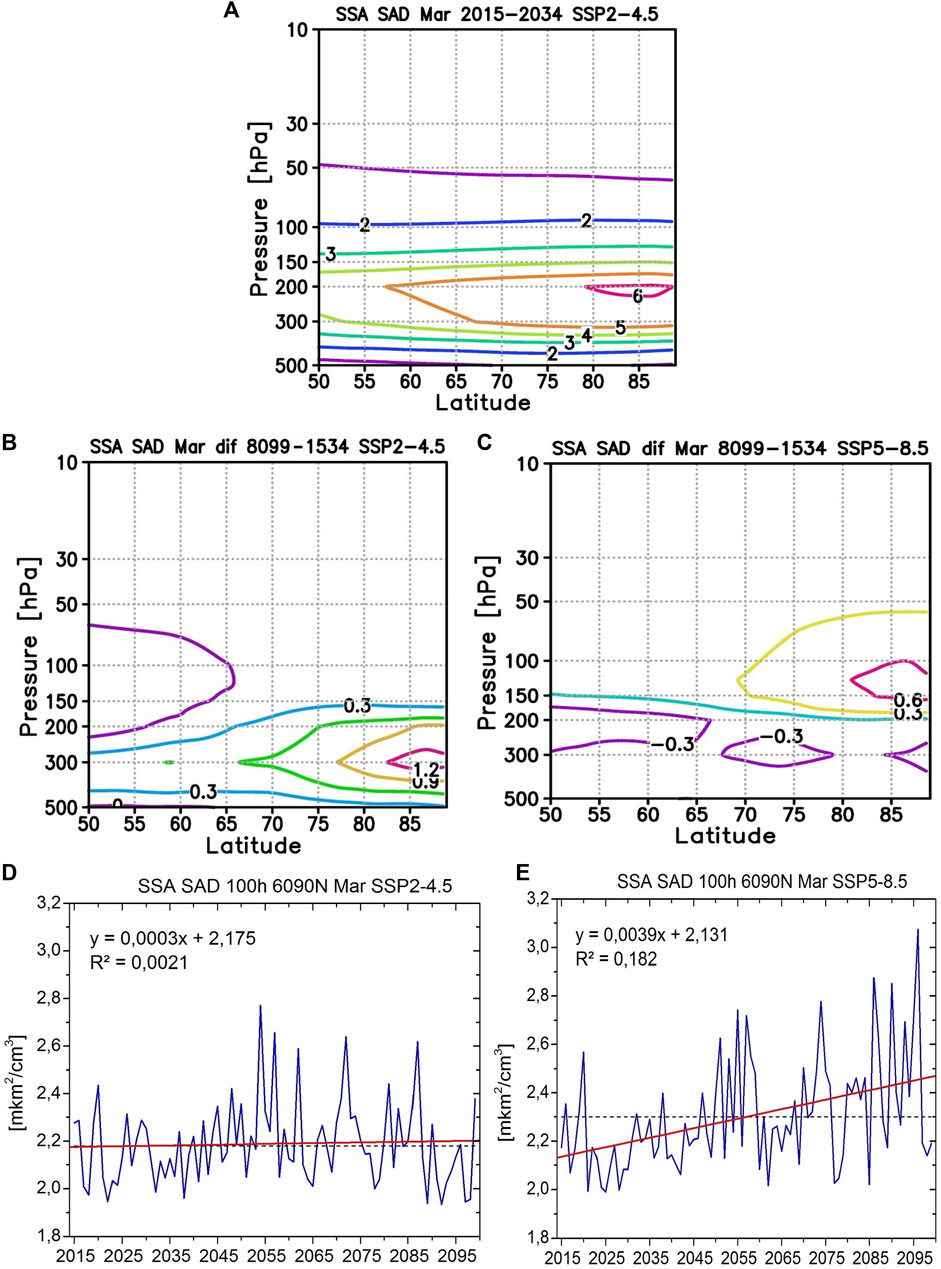
FIGURE 10. (A) Ensemble mean SSA SAD (mkm²/cm³) averaged over 60°N–90°N in March for the 2015–2034 period from the run driven by the SSP2–4.5 scenario. The difference (mkm²/cm³) between this quantity in 2080–2099 and 2015–2034 for the SSP2–4.5 (B) and the SSP5–8.5 (C) scenarios. SSA SAD averaged over 60°N–90°N at the pressure level 100 hPa in March from 2015 to 2099 for the SSP2–4.5 (D) and the SSP5–8.5 (E) scenarios.

The SSA SAD depends on the implied emission scenarios, stratospheric temperature, the intensity of the Brewer–Dobson circulation transporting tropospheric air to the stratosphere, and the state of the polar vortices which affects the isolation of the polar area in winter and early springtime. Because the five-fold decline of the sulfur-containing species emissions is almost identical under both scenarios (Gidden et al., 2019), different tendencies can be explained only by dynamical changes.

From the point of view of total column ozone depletion, the most significant is the atmospheric level which is approximately 100 hPa, where the ozone mixing ratio is still substantial and its depletion can be seen in the total ozone data. The changes in SSA SAD are presented in Figure 10D, E. Ensemble mean in the Arctic lower stratosphere in March throughout the 21st century is characterized by strong interannual variability under both scenarios. The statistically significant long-term SSA SAD trend appears only under the severe GHG emission scenario. Most probably, it is explained by the cooler stratosphere due to GHG concentration increase for the SSP5–8.5 scenario. However, this increase is not high enough to provide substantial total ozone depletion (Figure 11) and compete with other processes.

FIGURE 11

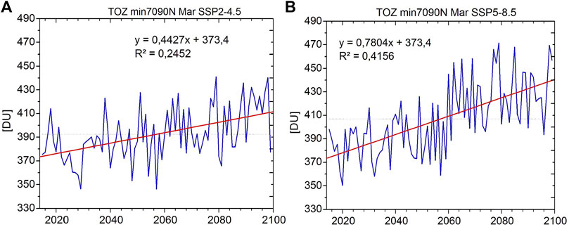
FIGURE 11. Minimal total ozone (TOZ) values in the polar cap (70°N–90°N) in March from 2015 to 2099 for the ensemble mean under SSP2–4.5 (A) and SSP5.8–5 (B) scenarios. The red straight line corresponds to the linear trend.

3.7 Future Arctic winters with the lowest polar cap total ozone in March

Model estimates show that Arctic springtime total ozone is expected to return to pre-1980 values slightly before mid-century (about 2045) (WMO, 2022). Total ozone minimum values inside the Arctic polar cap in March throughout the 21st century in SOCOLv4 simulations are characterized by a positive significant trend under both scenarios (Figure 11). It is consistent with results of SOCOLv4 simulation analysis, which showed that the total column ozone is expected to be distinctly higher than present in mid-to-high latitudes in both future scenarios (Karagodin-Doyennel et al., 2023).

However, substantial ozone loss occurs in cold winters in the Arctic stratosphere as long as concentrations of ozone-depleting substances are well above natural levels.

As it was mentioned previously, the largest ozone layer depletion with monthly mean negative total ozone large-scale anomalies in the Arctic over recent more than 40 years were observed in March 2011 with the values below −100 DU and in March 2020 with the values below −150 DU relative to 1991–2020 mean (Figure 12A, B).

FIGURE 12

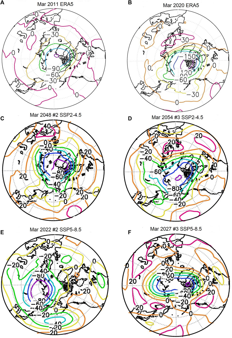
FIGURE 12. Total column ozone anomalies in March 2011 and in March 2020 in ERA5 reanalysis data (A, B). Largest negative total column ozone anomalies (DU) in March 2048 (experiment #2) and March 2054 (#3) under the SSP2–4.5 scenario (C, D); in March 2022 (#2) and in March 2027 (#3) under the SSP5–8.5 (E, F) scenario.

Analysis of minimum total ozone values in SOCOLv4 simulations throughout the 21st century revealed eight events with the lowest values of 300 DU–320 DU in the polar region (70°N–90°N) in March. Except for 1 year (2028 of experiment #2 under the SSP2–4.5 scenario), all of these events are characterized by large January–March mean Vpsc that significantly exceed the January–March mean value averaged over 2015–2099 of ∼15 mln cub km. Hereafter, these Vpsc values that are indicated in the brackets before the experiment number indicated by #: 2026 (Vpsc=24.5) #1, 2028 (14.4), 2045 (27.3), 2048 (57) #2, 2054 (53), and 2062 (74.4) #3 were revealed under the SSP2–4.5 scenario and two events 2022 (30) #2 and 2027 (52) #3 under the SSP5–8.5 scenario. The year of 2028 #2 under the SSP2–4.5 scenario with slightly less January–March mean Vpsc than climatological mean over 2015–2099 is characterized by large March mean Vpsc value ∼19 mln cub km. Therefore, it is plausible that all revealed large March negative anomalies in the Arctic in the SOCOLv4 simulation throughout the 21st century and comparable to second large ozone loss observed in March 2011 were due to chemical ozone loss, which in turn was caused by ozone-depleting compound transformation into active forms on the PSC particles.

Corresponding negative monthly mean total ozone anomalies reached up to -80–100 DU and were calculated relative to values averaged over the period of modern climate from 2001 to 2020. As an example, the total ozone anomalies of March 2048 (#2) and of March 2054 (#3) in SSP2–4.5 March 2022 (#2) and March 2027 (#3) in SSP5–8.5 are plotted in Figure 12C-F. The other four events (2026 #1, 2028, 2045 #2, and 2062 #3) under the SSP2–4.5 scenario are plotted in Supplementary Figures S8A-D.

The obtained results show that large-scale negative ozone anomalies in March comparable to the second lowest ones observed in March 2011, although weaker than record values observed in March 2020, are possible in the Arctic throughout the 21st century. All such anomalies were revealed in the SOCOLv4 simulations in the first part of the investigated period.

A comparison of the March total ozone in the polar region between averaged values over the 2080–2099 and 2015–2034 time periods shows its increase in the Arctic on 20–30 DU and 40–50 DU under SSP2–4.5 and SSP5–8.5 scenarios, respectively (Supplementary Figures S8E, F).

Notably, the large total ozone anomalies in the polar latitudes in March in some years persisted until April, for instance, in the year of 2048 of the experiment #2 and in the year of 2054 of the experiment #3 under the SSP2–4.5 scenario with the lowest negative anomalies exceeded −80 DU relative to the mean of 2001–2020 (Supplementary Figures S8G, H).

4 Discussion and conclusion

This study presents the evaluation of Arctic stratosphere dynamics and chemistry composition changes relevant to the ozone layer throughout the 21st century in two simulations consisting of three ensemble members and performed by CCM SOCOLv4 under the moderate SSP2–4.5 and severe SSP5–8.5 scenarios. Our analysis is mostly focused on changes in March because this month is characterized by the largest chemical ozone loss due to the higher solar zenith angle and enhanced penetration of solar radiation to the Arctic lower stratosphere after the polar night. However, if the cold and persistent stratospheric polar vortex with PSCs inside shifted off the pole in February, the inert reservoir species like HCl, HBr, and ClONO₂ are converted to Cl₂, ClBr, and ClNO₂ and transformed into active forms on the surface of PSC’s particles in the presence of solar light, and the chemical ozone loss could start before the beginning of March. Therefore, a more detailed analysis of the polar vortex changes is desirable using daily data. In addition, possible changes in the mid-winter sudden stratospheric warming and final stratospheric warming event characteristics (dates, lasting, with shift or splitting of the polar vortex, and influence on the lower stratosphere and troposphere) require daily data and, therefore, are beyond the scope of the present study.

A cooling of the stratosphere, related to GHG concentration increase, affects the zonal circulation and planetary wave propagation throughout the 21st century. Obtained estimates show a possible increase of upward planetary wave propagation, characterized by zonal mean meridional heat flux and the increase of wavenumber 1 amplitude dominated in the stratosphere under the moderate scenario over the high northern latitudes. Under the severe scenario, the upward planetary wave propagation does not show a comparable increase and the wavenumber 1 amplitude displays a weaker increase over middle and high latitudes and decrease over the polar latitudes in the late 21st century.

For the late 21st century, there is a good agreement between obtained estimates showing an increase of air volume with temperatures below the PSC formation threshold (especially in the SSP5–8.5 scenario) and results of previous analysis of CMIP6 model analysis (von der Gather et al., 2021) and the INM CM5 simulations (Vargin et al., 2022). In addition, the strengthening of the MPVG revealed in the high-latitude lower stratosphere for the late 21st century under both scenarios corresponds to a decrease in effective diffusivity at the polar vortex boundary and to an increase in its isolation. Therefore, our results give an evidence of a possibility of strengthening of the Arctic polar vortex in the lower stratosphere in March in the late 21st century in comparison with its beginning.

The largest total ozone-negative anomalies observed in the Arctic, comparable to those seen in March 2011 and March 2020, are projected to be possible in the future: six/two such events were revealed under the SSP2–4.5/SSP5–8.5 scenarios. All such March months were obtained in model simulations not later than 2076. This result is in agreement with the total ozone increases in the polar regions, with a slightly higher intensity under the SSP5–8.5 scenario revealed in SOCOLv4 simulations by Karagodin-Doyennel et al. (2023).

The polar vortex longitudinal shift toward northern Eurasia with the magnitude of the shift, increasing for larger global warming levels, is expected in the lower stratosphere in the late 21st century in both scenarios, which is in agreement with results of Zhang et al. (2020) and Karpechko et al. (2022). This polar vortex longitudinal shift can be interpreted as an eastward shift of the climatological wavenumber 1.

Presumably, the less favorable conditions in the extratropical stratosphere (that are, in turn, caused by wave–flow interaction changes) are responsible for weaker wave activity, characterized by less zonal mean heat flux and wave number 1 amplitude in January–February at the end of the 21st century under the SSP5–8.5 scenario in comparison with SSP2–4.5. However, further analysis is needed to estimate the possible impact of tropospheric sources on wave activity changes. Certainly, the larger number of ensemble members will allow to verify obtained estimates and improve its robustness on wave activity changes throughout the 21st century. Detailed analysis of global-scale wave structures, including their sources, and even possible changes in nonlinear interactions are outside the scope of this study and are subject to further investigation.

Overall, the following main conclusions can be drawn from the present study:

1. Cooling of the stratosphere due to GHG concentration growth is expected under both scenarios (larger in SSP5–8.5) in the late 21st century.

2. The cooling of the stratospheric temperature and strengthening of RMC will be accompanied by the zonal mean zonal wind increase up to 1–2 m/s under the moderate scenario and up to 6 m/s under the severe scenario.

3. The strengthening of upward wave activity propagation as well as of wavenumber 1 amplitude is expected under the moderate scenario in January–February. The severe scenario is characterized by a slight increase of wavenumber 2 amplitude in the late 21st century.

4. In the lower stratosphere, the polar vortex shift toward northern Eurasia is expected under both scenarios.

5. Increase of Vpsc in March is expected in both scenarios (with the larger in the SSP5–8.5) throughout the 21st century. Furthermore, the strengthening of the MGPV revealed in the middle stratosphere under both scenarios corresponds to a decrease in effective diffusivity at the vortex boundary and to an increase in the polar vortex isolation. These changes correspond to the strengthening of the Arctic polar vortex in the lower stratosphere and could lead to the strengthening of the chemical ozone loss at the late 21st century.

6. Due to favorable dynamical conditions, the strong ozone layer depletion is possible in the Arctic lower stratosphere, with the negative anomalies up to −80 DU–100 DU and comparable to observed ones in March 2011 but weaker than the ones observed in March 2020. Eight such events were revealed in the SOCOLv4 simulations under the moderate and severe scenarios.

7. Increase of humidity in the Arctic lower stratosphere in March up to 10% and 20% was revealed under the moderate and severe scenarios, respectively. Probably, a more pronounced SWV positive trend under the SSP5–8.5 scenario is related to stronger tropospheric water vapor influx into the stratosphere and enhanced production from CH₄ oxidation.

8. The statistically significant long-term stratospheric sulfuric acid aerosols/supercooled ternary solution (SSA/STS SAD) trend is expected only under the SSP5.8–5 scenario, most probably due to the cooler stratosphere. However, this increase will be unable to lead to substantial total ozone depletion.

Finally, this study highlights the importance of estimation of Arctic stratospheric polar vortex dynamics and chemistry composition characteristics averaged within the vortex boundary in comparison with the analysis of the same characteristics averaged over the entire polar cap. In the latter case, obtained estimates could lead to misleading conclusions and did not show a possible large seasonal loss of Arctic ozone throughout the 21st century (von der Gathen et al., 2023).

However, unpredictable possible changes in interannual variability of extratropical Arctic stratosphere dynamical processes (first of all, wave activity and its interaction with zonal circulation) throughout the 21st century as well as the larger number of analyzed ensemble members could affect obtained estimates.

Data availability statement

The raw data supporting the conclusion of this article will be made available by the authors, without undue reservation.

Author contributions

PV, SK, AK, ER, TE, SS, and NT had valuable contribution in writing and editing of the text, data analysis, and visualization of the results, including in providing the data of climate modeling (ER), investigation of stratospheric circulation, wave activity, and composition changes (PV, ER, SS, TE, and NT), the calculation of the PSC volume and the analysis of its changes (SK), and the calculation of the residual meridional circulation and corresponding alteration of meridional fluxes of mass and the analysis of its changes (AK). All authors contributed to the article and approved the submitted version.

Funding

The study was performed at the ‟Laboratory for the Research of the Ozone Layer and the Upper Atmosphere” of Saint Petersburg State University and Russian State Hydrometeorological University under the state task of the Ministry of Science and Higher Education and was funded by the Government of the Russian Federation under agreement [075-15-2021-583] and state task project FSZU-2023-0002.

Acknowledgments

The reanalysis Era5 data were provided: y ECMWF through the Climate Data Store https://cds.climate.copernicus.eu (accessed on April 6, 2023). All plots in this study were made using the Grid Analysis and Display System (GrADS), which is a free software developed thanks to the NASA Advanced Information Systems Research Program.

Conflict of interest

The authors declare that the research was conducted in the absence of any commercial or financial relationships that could be construed as a potential conflict of interest.

Publisher’s note

All claims expressed in this article are solely those of the authors and do not necessarily represent those of their affiliated organizations, or those of the publisher, the editors, and the reviewers. Any product that may be evaluated in this article, or claim that may be made by its manufacturer, is not guaranteed or endorsed by the publisher.

Supplementary material

The Supplementary Material for this article can be found online at: https://www.frontiersin.org/articles/10.3389/feart.2023.1214418/full#supplementary-material

References

Abalos, M., Calvo, N., Benito-Barca, S., Garny, H., Hardiman, S. C., Lin, P., et al. (2021). The brewer–dobson circulation in CMIP6. Atmos. Chem. Phys. 21, 13571–13591. doi:10.5194/acp-21-13571-2021

CrossRef Full Text | Google Scholar

Akiyoshi, H., Kadowaki, M., Yamashita, Y., and Nagatomo, T. (2023). Dependence of column ozone on future ODSs and GHGs in the variability of 500-ensemble members. Sci. Rep. 13, 320. doi:10.1038/s41598-023-27635-y

PubMed Abstract | CrossRef Full Text | Google Scholar

Andersson, S. M., Martinsson, B. G., Vernier, J.-P., Friberg, J., Brenninkmeijer, C. A., Hermann, M., et al. (2015). Significant radiative impact of volcanic aerosol in the lowermost stratosphere. Nat. Commun. 6, 7692. doi:10.1038/ncomms8692

PubMed Abstract | CrossRef Full Text | Google Scholar

Andrews, D. G., and McIntyre, M. E. (1976). Planetary waves in horizontal and vertical shear: The generalized Eliassen–Palm relation and the mean zonal acceleration. J. Atmos. Sci. 33, 2031–2048. doi:10.1175/1520-0469(1976)033<2031:PWIHAV>2.0

CrossRef Full Text | Google Scholar

Austin, J., Shindell, D., Beagley, S. R., Brühl, C., Dameris, M., Manzini, E., et al. (2003). Uncertainties and assessments of chemistry-climate models of the stratosphere. Atmos. Chem. Phys. 3, 1–27. doi:10.5194/acp-3-1-2003

CrossRef Full Text | Google Scholar

Baldwin, M., Birner, T., Brasseur, G., Burrows, J., Butchart, N., Garcia, R., et al. (2019). 100 Years of progress in understanding the stratosphere and mesosphere. Meteorol. Monogr. 59, 27.1–27.62. 1–27. doi:10.1175/AMSMONOGRAPHS-D-19-0003.1

CrossRef Full Text | Google Scholar

Ball, W. T., Alsing, J., Mortlock, D. J., Staehelin, J., Haigh, J. D., Peter, T., et al. (2018). Evidence for a continuous decline in lower stratospheric ozone offsetting ozone layer recovery. Atmos. Chem. Phys. 18, 1379–1394. doi:10.5194/acp-18-1379-2018

CrossRef Full Text | Google Scholar

Butchart, N., Cionni, I., Eyring, V., Shepherd, T., Waugh, D., Akiyoshi, H., et al. (2010). Chemistry-climate model simulations of twenty-first century stratospheric climate and circulation changes. J. Clim. 23, 5349–5374. doi:10.1175/2010JCLI3404.1

CrossRef Full Text | Google Scholar

Butchart, N. (2022). The stratosphere: A review of the dynamics and variability. Weather Clim. Dynam. 3, 1237–1272. doi:10.5194/wcd-3-1237-2022

CrossRef Full Text | Google Scholar

Carslaw, K. S., Luo, B. P., and Peter, T. (1995). An analytic expression for the composition of aqueous HNO3-H2SO4 stratospheric aerosols including gas-phase removal of HNO3. Geophys. Res. Lett. 22, 1877–1880. doi:10.1029/95gl01668

CrossRef Full Text | Google Scholar

Chipperfield, M. (2009). Atmospheric science: Nitrous oxide delays ozone recovery. Nat. Geosci. 2, 742–743. doi:10.1038/ngeo678

CrossRef Full Text | Google Scholar

Chipperfield, M., Bekki, S., Dhomse, S., Harris, N., Hassler, B., Hossaini, R., et al. (2017). Detecting recovery of the stratospheric ozone layer. Nature 549, 211–218. doi:10.1038/nature23681

PubMed Abstract | CrossRef Full Text | Google Scholar

Chipperfield, M. P., Dhomse, S., Hossaini, R., Feng, W., Santee, M. L., Weber, M., et al. (2018). On the cause of recent variations in lower stratospheric ozone. Geophys. Res. Lett. 45, 5718–5726. doi:10.1029/2018GL078071

CrossRef Full Text | Google Scholar

Dessler, A. E., Schoeberl, M. R., Wang, T., Davis, S. M., and Rosenlof, K. H. (2013). Stratospheric water vapor feedback. P. Natl. Acad. Sci. U. S. A. 110, 18087–18091. doi:10.1073/pnas.1310344110

CrossRef Full Text | Google Scholar

Fleming, E. L., Newman, P. A., Liang, Q., and Daniel, J. S. (2020). The impact of continuing CFC-11 emissions on stratospheric ozone. J. Geophys. Res.-Atmos. 125, e31849. doi:10.1029/2019JD031849

CrossRef Full Text | Google Scholar

Garcia, R. R., and Randel, W. J. (2008). Acceleration of the Brewer-Dobson circulation due to increases in greenhouse gases. J. Atmos. Sci. 65 (8), 2731–2739. doi:10.1175/2008JAS2712.1

CrossRef Full Text | Google Scholar

Gečaitė, I. (2021). Climatology of three-dimensional eliassen–PalmWave activity fluxes in the northern hemisphere stratosphere from 1981 to 2020. Climate 9, 124. doi:10.3390/cli9080124

CrossRef Full Text | Google Scholar

Gelaro, R., McCarty, W., Suárez, M. J., Todling, R., Molod, A., Takacs, L., et al. (2017). The modern-era retrospective analysis for research and applications, version 2 (MERRA-2). J. Clim. 30, 5419–5454. doi:10.1175/JCLI-D-16-0758.1

CrossRef Full Text | Google Scholar

Gidden, M. J., Riahi, K., Smith, S. J., Fujimori, S., Luderer, G., Kriegler, E., et al. (2019). Global emissions pathways under different socioeconomic scenarios for use in CMIP6: A dataset of harmonized emissions trajectories through the end of the century. Geosci. Model. Dev. 12, 1443–1475. doi:10.5194/gmd-12-1443-2019

CrossRef Full Text | Google Scholar

Giorgetta, M. A., Manzini, E., Roeckner, E., Esch, M., and Bengtsson, L. (2016). Climatology and forcing of the quasi-biennial oscillationin the MAECHAM5 model. J. Clim. 19, 3882–3901. doi:10.1175/JCLI3830.1

CrossRef Full Text | Google Scholar

Giorgetta, M., Jungclaus, J., Reick, C., Legutke, S., Bader, J., Böttinger, M., et al. (2013). Climate and carbon cycle changes from 1850 to 2100 in MPI-ESM simulations for the coupled model intercomparison project phase 5: Climate changes in MPI-ESM. J. Advan. Model. Earth Syst. 5, 572–597. doi:10.1002/jame.20038

CrossRef Full Text | Google Scholar

Haase, S., and Matthes, K. (2019). The importance of interactive chemistry for stratosphere–troposphere coupling. Atmos. Chem. Phys. 19, 3417–3432. doi:10.5194/acp-19-3417-2019

CrossRef Full Text | Google Scholar

Hanson, D., and Mauersberger, K. (1988). Laboratory studies of the nitric acid trihydrate: Implications for the south polar stratosphere. Geophys. Res. Lett. 15, 855–858. doi:10.1029/gl015i008p00855

CrossRef Full Text | Google Scholar

Karagodin-Doyennel, A., Rozanov, E., Sukhodolov, T., Egorova, T., Sedlacek, J., and Peter, T. (2023). The future ozone trends in changing climate simulated with SOCOLv4. EGUsphere. doi:10.5194/egusphere-2022-1260

CrossRef Full Text | Google Scholar

Karagodin-Doyennel, A., Rozanov, E., Sukhodolov, T., Egorova, T., Saiz-Lopez, A., Cuevas, C. A., et al. (2021). Iodine chemistry in the chemistry–climate model SOCOL-AERv2-I. Geosci. Model. Dev. 14, 6623–6645. doi:10.5194/gmd-14-6623-2021

CrossRef Full Text | Google Scholar

Karagodin-Doyennel, A., Rozanov, E., Sukhodolov, T., Egorova, T., Sedlacek, J., Ball, W., et al. (2022). The historical ozone trends simulated with the SOCOLv4 and their comparison with observations and reanalyses. Atmos. Chem. Phys. 22, 15333–15350. doi:10.5194/acp-22-15333-2022

CrossRef Full Text | Google Scholar

Karpechko, A. Yu., Afargan-Gerstman, H., Butler, A., Domeisen, D. I. V., Kretschmer, M., Lawrence, Z., et al. (2022). Northern hemisphere stratosphere-troposphere circulation change in CMIP6 models: 1. Inter-model spread and scenario sensitivity. J. Geophys. Res. Atmos. 127 (18). e2022JD036992. doi:10.1029/2022jd036992

CrossRef Full Text | Google Scholar

Keeble, J., Banerjee, A., Chiodo, G., Hassler, B., Banerjee, A., Checa-Garcia, R., et al. (2021). Evaluating stratospheric ozone and water vapour changes in CMIP6 models from 1850 to 2100. Atmos. Chem. Phys. 21, 5015–5061. doi:10.5194/acp-21-5015-2021

CrossRef Full Text | Google Scholar

Kostrykin, S. V., and Schmitz, G. (2006). Effective diffusivity in the middle atmosphere based on general circulation model winds. J. Geophys. Res. 111, D02304. doi:10.1029/2004jd005472

CrossRef Full Text | Google Scholar

Koval, A. V., Chen, W., Didenko, K. A., Ermakova, T. S., Gavrilov, N. M., Pogoreltsev, A. I., et al. (2021). Modelling the residual mean meridional circulation at different stages of sudden stratospheric warming events. Ann. Geophys. 39, 357–368. doi:10.5194/angeo-39-357-2021

CrossRef Full Text | Google Scholar

Lawrence, Z. D., Manney, G. L., Minschwaner, K., Santee, M. L., and Lambert, A. (2015). Comparisons of polar processing diagnostics from 34 years of the ERA-Interim and MERRA reanalyses. Atmos. Chem. Phys. 15, 3873–3892. doi:10.5194/acp-15-3873-2015

CrossRef Full Text | Google Scholar

Lawrence, Z., Wargan, K., Manney, G., , and Wargan, K. (2018). Reanalysis intercomparisons of stratospheric polar Reanalysis intercomparisons of stratospheric polar processing diagnostics. Atmos. Chem. Phys. 18, 13547–13579. doi:10.5194/acp-18-13547-2018

PubMed Abstract | CrossRef Full Text | Google Scholar

Matsumura, S., Yamazaki, K., and Horinouchi, T. (2021). Robust asymmetry of the future Arctic polar vortex is driven by tropical Pacific warming. Geophys. Res. Lett. 48 (11), e2021GL093440. doi:10.1029/2021GL093440

CrossRef Full Text | Google Scholar

Matthes, K., Funke, B., Andersson, M. E., Barnard, L., Beer, J., Charbonneau, P., et al. (2017). Solar forcing for CMIP6 (v3.2). Geosci. Model. Dev. 10 (6), 2247–2302. doi:10.5194/gmd-10-2247-2017

CrossRef Full Text | Google Scholar

Newman, P. A., Nash, E. R., and Rosenfeld, J. E. (2001). What controls the temperature of the Arctic stratosphere during the spring? J. Geophys. Res. 106 (D17), 19999–20010. doi:10.1029/2000JD000061

CrossRef Full Text | Google Scholar

Oberländer, S., Langematz, U., and Meul, S. (2013). Unraveling impact factors for future changes in the Brewer-Dobson circulation. J. Geoph. Res. Atmos. 118, 10296–10312. doi:10.1002/jgrd.50775

CrossRef Full Text | Google Scholar

Oram, D. E., Ashfold, M. J., Laube, J. C., Gooch, L. J., Humphrey, S., Sturges, W. T., et al. (2017). A growing threat to the ozone layer from short-lived anthropogenic chlorocarbons. Atmos. Chem. Phys. 17, 11929–11941. doi:10.5194/acp-17-11929-2017

CrossRef Full Text | Google Scholar

Plumb, R. (1985). On the three-dimensional propagation of stationary waves. J. Atmos. Sci. 42, 217–229. doi:10.1175/1520-0469(1985)042<0217:ottdpo>2.0.co;2

CrossRef Full Text | Google Scholar

Revell, L. E., Bodeker, G. E., Huck, P. E., Williamson, B. E., and Rozanov, E. (2012). The sensitivity of stratospheric ozone changes through the 21st century to N₂O and CH₄. Atmos. Chem. Phys. 12, 11309–11317. doi:10.5194/acp-12-11309-2012

CrossRef Full Text | Google Scholar

Riahi, K., van Vuuren, D. P., Kriegler, E., Edmonds, J., O’Neill, B. C., Fujimori, S., et al. (2017). The Shared Socioeconomic Pathways and their energy, land use, and greenhouse gas emissions implications: An overview. Glob. Environ. Change 42, 153–168. doi:10.1016/j.gloenvcha.2016.05.009

CrossRef Full Text | Google Scholar

Rieder, H., Chiodo, G., Fritzer, J., Wienerroither, C., and Polvani, L. (2019). Is interactive ozone chemistry important to represent polar cap stratospheric temperature variability in Earth-System Models? Environ. Res. Lett. 14, 044026. doi:10.1088/1748-9326/ab07ff

CrossRef Full Text | Google Scholar

Salawitch, R. J., Wofsy, S. C., Gottlieb, E. W., Lait, L. R., Newman, P. A., Schoeberl, M. R., et al. (1993). Chemical loss of ozone in the Arctic polar vortex in the winter of 1991–1992. Science 261, 1146–1149. doi:10.1126/science.261.5125.1146

PubMed Abstract | CrossRef Full Text | Google Scholar

Shepherd, T. G. (2007). Transport in the middle atmosphere. J. Meteorol. Soc. Jpn. 85B, 165–191. doi:10.2151/jmsj.85b.165

CrossRef Full Text | Google Scholar

Steiner, A. K., Ladstädter, F., Randel, W. J., Maycock, A. C., Fu, Q., Claud, C., et al. (2020). Observed temperature changes in the troposphere and stratosphere from 1979 to 2018. J. Clim. 33, 8165–8194. doi:10.1175/JCLI-D-19-0998.1

CrossRef Full Text | Google Scholar

Steiner, M., Luo, B., Peter, T., Pitts, M., and Stenke, A. (2021). Evaluation of polar stratospheric clouds in the global chemistry–climate model SOCOLv3.1 by comparison with CALIPSO spaceborne lidar measurements Geosci. Model Dev. Geosci. Model. Dev. 14, 935–959. doi:10.5194/gmd-14-935-2021

CrossRef Full Text | Google Scholar

Sukhodolov, T., Egorova, T., Stenke, A., Ball, W. T., Brodowsky, C., Chiodo, G., et al. (2021). Atmosphere–ocean–aerosol–chemistry–climate model SOCOLv4.0: Description and evaluation. Geosci. Model. Dev. 14, 5525–5560. doi:10.5194/gmd-14-5525-2021

CrossRef Full Text | Google Scholar

Tian, W., Chipperfield, M. P., and Lü, D. (2009). Impact of increasing stratospheric water vapor on ozone depletion and temperature change. Adv. Atmos. Sci. 26 (3), 423–437. doi:10.1007/s00376-009-0423-3

CrossRef Full Text | Google Scholar

Tilmes, S., Müller, R., Engel, A., Rex, M., and Russell, J. M. (2006). Chemical ozone loss in the Arctic and Antarctic stratosphere between 1992 and 2005. Geophys. Res. Lett. 33, L20812. doi:10.1029/2006gl026925

CrossRef Full Text | Google Scholar

Urban, J., Pommier, M., Murtagh, D. P., Santee, M. L., and Orsolini, Y. J. (2009). Nitric acid in the stratosphere based on odin observations from 2001 to 2009 – Part 1: A global climatology. Atmos. Chem. Phys. 9, 7031–7044. doi:10.5194/acp-9-7031-2009

CrossRef Full Text | Google Scholar

Vargin, P. N., Kostrykin, S. V., Volodin, E. M., Pogoreltsev, A. I., and Wei, K. (2022). Arctic stratosphere circulation changes in the 21st century in simulations of INM CM5. Atmosphere 13 (1), 25. doi:10.3390/atmos13010025

CrossRef Full Text | Google Scholar

Vargin, P. N., Коstrykin, S. V., Rakushina, Е. V., Volodin, Е. М., and Pogoreltzev, А. I. (2020). Investigation of variability of Spring Breakup dates and Arctic stratospheric polar vortex parameters in modeling and reanalysis data. Izv. Atmos. Ocean. Phys. 56, 526–539. doi:10.1134/S0001433820050114

CrossRef Full Text | Google Scholar

von der Gathen, P., Kivi, R., Wohltmann, I., Salawitch, R. J., and Rex, M. (2023). Reply to: No evidence of worsening arctic springtime ozone losses over the 21st century. Nat. Commun. 14, 1609. doi:10.1038/s41467-023-37135-2

PubMed Abstract | CrossRef Full Text | Google Scholar

von der Gathen, P., Kivi, R., Wohltmann, I., Salawitch, R., and Rex, M. (2021). Climate change favours large seasonal loss of Arctic ozone. Nat. Commun. 12, 3886–3917. doi:10.1038/s41467-021-24089-6

PubMed Abstract | CrossRef Full Text | Google Scholar

Wang, W., Tian, W., Dhomse, S., Xie, F., Shu, J., and Austin, J. (2014). Stratospheric ozone depletion from future nitrous oxide increases. Atmos. Chem. Phys. 14, 12967–12982. doi:10.5194/acp-14-12967-2014

CrossRef Full Text | Google Scholar

Waugh, D. (2009). The age of stratospheric air. Nat. Geosci. 2, 14–16. doi:10.1038/ngeo397

CrossRef Full Text | Google Scholar

Wegner, T., Groos, J.-U., von Hobe, M., Stroh, F., Sumińska-Ebersoldt, O., Volk, C. M., et al. (2012). Heterogeneous chlorine activation on stratospheric aerosols and clouds in the arctic polar vortex. Atmos. Chem. Phys. 12, 11095–11106. doi:10.5194/acp-12-11095-2012

CrossRef Full Text | Google Scholar

Wei, K., Ma, J., Chen, W., and Vargin, P. (2021). Longitudinal peculiarities of planetary waves-zonal flow interactions and their role in stratosphere-troposphere dynamical coupling. Clim. Dyn. 57, 2843–2862. doi:10.1007/s00382-021-05842-5

CrossRef Full Text | Google Scholar

Wilks, D. S. (2006). Statistical methods in the atmospheric sciences Oxford: Elsevier.

Google Scholar

WMO. Executive summary of scientific assessment of ozone depletion. 2022. WMO: Geneva, Switzerland.

Google Scholar

Zhang, J., Tian, W., Chipperfield, M. P., Xie, F., and Huang, J. (2016). Persistent shift of the Arctic polar vortex towards the eurasian continent in recent decades. Nat. Clim. Change 6, 1094–1099. doi:10.1038/nclimate3136

CrossRef Full Text | Google Scholar

Zhang, J., Tian, W., Pyle, J. A., Keeble, J., Abraham, N. L., Chipperfield, M. P., et al. (2022). Responses of Arctic sea ice to stratospheric ozone depletion. Sci. Bull. 67 11, 1182–1190. doi:10.1016/j.scib.2022.03.015

CrossRef Full Text | Google Scholar

Zhang, J., Tian, W., Xie, F., Chipperfield, M., Feng, W., Son, S.-W., et al. (2018). Stratospheric ozone loss over the Eurasian continent induced by the polar vortex shift. Nat. Commun. 9, 206. doi:10.1038/s41467-017-02565-2

PubMed Abstract | CrossRef Full Text | Google Scholar

Zhang, J., Tian, W., Xie, F., Pyle, J. A., Keeble, J., and Wang, T. (2020). The influence of zonally asymmetric stratospheric ozone changes on the arctic polar vortex shift. J. Clim. 33 (11), 4641–4658. doi:10.1175/JCLI-D-19-0647.1

CrossRef Full Text | Google Scholar

Zhao, S., Yu, Y., Lin, P., Liu, H., He, B., Bao, Q., et al. (2020). Datasets for the CMIP6 scenario model intercomparison project (ScenarioMIP) simulations with the coupled model CAS FGOALS-f3-L. Adv. Atmos. Sci. 38, 329–339. doi:10.1007/s00376-020-0112-9

CrossRef Full Text | Google Scholar

Zubov, V., Rozanov, E., Egorova, T., Karol, I., and Schmutz, W. (2013). Role of external factors in the evolution of the ozone layer and stratospheric circulation in 21st century. Atmos. Chem. Phys. 13, 4697–4706. doi:10.5194/acp-13-4697-2013

CrossRef Full Text | Google Scholar