Different methods of estimating riverbed sediment grain size diverge at the basin scale

Introduction: The distribution of sediment grain size in streams and rivers is often quantified by the median grain size (D50), a key metric for understanding and predicting hydrologic and biogeochemical function of streams and rivers. Manual D50 measurements are time-consuming and ignore larger grains, while approaches to model D50 based on catchment characteristics may over-generalize and miss site-scale heterogeneity. Machine learning-enabled object detection methods like You Only Look Once (YOLO) provides an alternative that enables estimation of D50 that is faster than manual measurements and more site-specific than predictions based on catchment characteristics.

Methods: To understand the potential role of object detection methods for improving understanding of D50, we compared D50 estimates made manually, predicted from catchment characteristics, and using a YOLO-enabled approach across the Yakima River Basin.

Results: We found distinct differences between methods for D50 averages and variability, and relationships between D50 estimates and basin characteristics.

Discussion: We discuss the advantages and limitations of object detection methods versus current methods, and explore potential future directions to combine D50 methods to better estimate spatiotemporal variation of D50, and improve incorporation into basin-scale models.

1 Introduction

The grain size distribution (GSD) of sediments in streams and rivers, often represented by the median of the GSD (D50), plays many important roles that regulate fluvial hydrology and biogeochemistry, and their interactions. Grains ranging from clays to boulders control the locations and rates of groundwater-surface water exchange, which can influence stream metabolism, as well as gas (e.g., oxygen and carbon dioxide) and solute sources, fate, and transport (Glaser et al., 2020; Gomez-Velez et al., 2015; Harvey et al., 2011; Mori et al., 2017; Son et al., 2022; Xia et al., 2017). Because of these roles, GSD is a key metric for predicting hydraulic conductivity (Wang et al., 2017), flow resistance (Rickenmann and Recking, 2011), microbial respiration and denitrification in streambeds (Buser-Young et al., 2023; Son et al., 2022), and parameterizing hydromorphological models (Lepesqueur et al., 2019). However, constraints on accurate assessment of D50 values at the basin scale, including uncertainty and bias associated with methods used to estimate D50 and the spatially and temporally sparse nature of current D50 data, limit our ability to accurately parameterize the models used to predict key basin functions.

Historic methods for determining D50 involve destructive sampling followed by manual counting or sieving procedures (Folk, 1966; Wolman, 1954). While these methods provide direct, site-specific measurements, they are time/labor-intensive with limited reproducibility and subject to variability depending on methods used (e.g., Lopez-Garcia et al., 2021; Poullet et al., 2019), making it difficult to provide sufficient spatiotemporal resolution needed to understand basin-scale heterogeneity of D50 (Mair et al., 2024). Manual methods also generally favor measuring smaller grains and ignore grains over a specific size cut-off, limiting the ability to characterize large grains. Recently developed methods such as processed-based and machine learning models have been used to estimate D50 values using basin characteristics from regional to continental scales (Abeshu et al., 2022; Gomez-Velez and Harvey, 2014; Ren et al., 2020). Both statistical and machine-learning model-based methods described above provide the advantage of continuous spatial coverage and eliminate the need for sample collection and analysis. However, these methods rely on assumed relationships that may have difficulty accounting for the high heterogeneity in predictor variables at smaller (site-to-reach) scales. Moreover, differences between methods or users can lead to high variability in D50 estimates (e.g., Faustini and Kaufmann, 2007).

Advances in object detection hold promise for bridging the gap between manual methods, which accurately characterize D50 across a small set of samples but are difficult to scale up to basin-scale, and watershed characteristics-based estimates, which provide large-scale estimates at the expense of site-scale accuracy. Object detection methods ingest images of sediments, and process them to estimate grain sizes, which can then be used to construct GSDs (Chang and Chung, 2012; Detert and Weitbrecht, 2020; Lang et al., 2021; Purinton and Bookhagen, 2019). Segmentation-based object detection approaches are increasingly coupled with machine learning algorithms to advance these methodologies (e.g., Chen et al., 2024; Detert and Weitbrecht, 2012; Purinton and Bookhagen, 2019; Steer et al., 2022), and have been shown to agree well with manual measurement methods (Stähly et al., 2017; Steer et al., 2022). They have several advantages over manual measurements which are highly localized in space, including non-destructive sampling, higher throughput, potential to automate analyses, and improved reproducibility. In addition, as estimates are based directly on information collected at a site, object detection-based D50 estimates contain more site-specific information compared to predictions based on catchment characteristics. Object detection methods may, therefore, fill a need for improved resolution and accuracy between physical and catchment characteristics-based methods. However, object detection methods remain sensitive to common environmental interferences to image processing such as shadows, water, and non-grain objects, are limited to surface sediments, and are susceptible to issues with image quality (e.g., non-vertical angles, glare, and blur).

In this study, we explore D50 estimates made using a process that includes the machine learning-enabled object detection algorithm called “You Only Look Once” (YOLO), described in detail in Chen et al. (2024), in comparison to other methods for estimating D50 across river basins. YOLO is one of a growing suite of machine learning image-based tools used in the process of estimating D50 (e.g., Buscombe, 2020; Chen et al., 2022; Mair et al., 2024) that holds potential to overcome limitations of other methods used to measure or estimate D50 described above. YOLO presents several potential advantages over other current object detection approaches, including rapid image processing, robustness to common environmental interferences like shadows, static and flowing water, and non-sediment-grain objects, and initial parameterization from a collection of public datasets, reducing the model’s prediction bias towards a specific location (Chen et al., 2024). To evaluate the utility of object detection methods for estimating D50, we analyzed 161 images collected on the banks of streams/rivers across 40 sites throughout the Yakima River Basin (YRB, Washington, United States). We compared D50 estimates enabled by YOLO object detection of these photos to manual D50 measurements made by the United States Geological Survey and D50 estimates predicted from catchment characteristics across the YRB. By exploring similarities and differences in average values, variance, and relationships to catchment characteristics, we revealed advantages and limitations of YOLO-enabled D50 estimation at the basin scale.

2 Methods

2.1 Site description and image collection

We selected 40 sites spread across the YRB in southern Washington State, United States to represent a range of D50 values across gradients of latitude, elevation, land use, and stream order (Strahler, 1964). The YRB is a 15,523 km² catchment characterized primarily by forests and grassland (28% and 26% respectively), as well as agriculture (15%) and a developed urban areas (3%) (Stroud Water Research Center, 2023). Streamflow throughout the YRB is regulated by five reservoirs storing approximately a third of annual runoff as well as considerable withdrawals for irrigation (Vano et al., 2010). Our sites span the headwaters to the main stem of the Yakima River, representing 2nd–7th order streams (Figure 1). The sites capture a wide range of grain sizes from small rocks and finer grains (Figure 1B) to large cobbles (Figure 1C). We also included one image collected nearby on the Columbia River (Figure 1A).

Figure 1

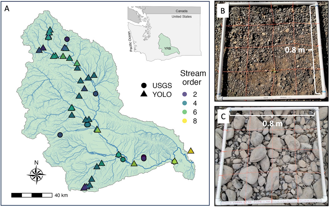
Figure 1. (A) A map of the Yakima River Basin (YRB) and sites where images used in this study were collected. Example photos (B,C) show the use of a quadrat to define the area of analysis for the YOLO object detection model, with (B) as an example of a streambed with smaller rocks/sand grains and (C) as an example of a streambed with larger cobbles.

During a sampling campaign in 2021, we collected 161 images used for estimating D50 at sites previously selected to encompass the range of biophysical and hydrologic characteristics found within the YRB, as determined via clustering analysis described in Fulton et al. (2022). For these photos we focused on materials that were obviously riverbed sediments (i.e., those that would normally be underwater during normal/seasonally high water, not the shoreline soils that would only be underwater during a large flood). The photo sites were selected between the water’s edge and the upper “scour line.” The scour line can be subjective, but typically there are obvious soils above it and little to no soil below it. Below the scour line, sediments are exposed due to water removing (i.e., scouring) soil. Photo locations selected were visually representative of the site’s general exposed sediments, based on the professional judgment of the sampling team, and relatively flat. Photos were taken at one or more locations at each site, during the day. At each location, a 0.8 m × 0.8 m white polyvinyl chloride pipe quadrat serving as the spatial reference frame was placed on the sediment, and photos were taken covering the area enclosed in the quadrat. At 34 of 40 sites, we collected multiple images to assess intra-site variability (ranging from 2 to 11). Original images are published as a data package stored on the ESS-DIVE repository (Fulton et al., 2022). We note that images are not capable of capturing information on grain size below the surface, which limits the ability to understand how grain sizes aggregate or change below the surface layer. Previous studies have shown changes in D50 with depth, including in sandy-bottom systems (e.g., Poullet et al., 2019), indicating this is an important consideration, though outside the scope of the current study’s methods. We also note that all methods compared in this study exclusively investigate surface sediments.

Prior to modeling, we visually assessed all images for potential environmental interferences, including shadows, wetting, sediment/biofilm obscuring grain edges, non-grain objects, and plants. Images were graded into one of four categories based on presence/absence of the above interferences: “Yes” (no substantial interference expected), “Maybe” (generally clear grains, but some potential interference”) and “No” (substantial interference expected). Grading is a subjective process and was therefore conducted by a single grader in a single session, with an average labor burden of 30 s per image.

2.2 Object detection-based D50 estimates

The object detection-based D50 estimates presented in this study are based on a machine learning modeling approach outlined in Chen et al. (2024). Briefly, we retrained You Look Only Once (YOLO, version 5) (Redmon et al., 2016) using 11,977 labels of grains collected from 9 typical stream environments using code accessed from https://github.com/ultralytics/yolov5 to identify grains as objects. Grains for training images were manually labeled by three annotators, then evaluated and corrected as necessary by a single annotator prior to ingestion by the model. Because speed of detection was not of concern in this study, we used the extra large-scale YOLO neural network. The structure of the YOLO neural networks are mainly connections of multiple convolutional neural networks (Zhang et al., 1990), modified bottleneck cross stage partial networks (Wang et al., 2019), spatial pyramid pooling fast layers (He et al., 2014), upsampling layers, and concatenated layers (https://pytorch.org/docs/stable/generated/torch.cat.html), where the full network included 476 layers and 87 million trainable parameters. We derived initial parameter values from a pre-trained network using the public YOLO COCO 128 datasets (accessed from https://cocodataset.org/). The model used a 59/8/33% split of images for training/validation/testing.

For each photo, we only considered the region within the quadrat, where each pixel along the vertical and horizontal lines of the quadrat represented a height and width. When pixels were averaged between height and width, we obtained an average image resolution ranging from 0.1 to 0.7 mm/pixel. Based on the model reported by Chen et al. (2024), we found a maximum ratio of detectable grain size to image resolution of 13 (average of 9, minimum of 4), meaning identifying a grain taking up less than 13 pixels could be affected by photo resolution. In our images, this suggests resolution could play a role for grain sizes ∼9.1 mm (13 pixels * 0.7 mm/pixel, our coarsest image resolution) or smaller. Chen et al. (2024) also reported that resolution varied linearly with camera height, where images taken less than 2 m above the ground would have a resolution of 0.7 mm/pixel or finer. For analyzed images (excluding training images), the model identified grains ranging from 1 to 955 mm. Grains were detected as individual objects by the YOLO model, which draws a bounding box around each object. The diagonal lengths of all detected objects were then used to estimate an area-weighted GSD, which we used to estimate a D50 value for each image. We refer to the D50 estimates made using this approach as the “YOLO” approach for simplicity throughout this manuscript, though we note that YOLO is not capable of directly estimating D50 but rather is one part of the process described in this section. Using labeled grains scaled to mm, we generated GSDs, and then calculated D50 values from each GSD. These data are publicly available on the ESS-DIVE repository (Regier et al., 2023), and a full description of our YOLO approach, including a detailed explanation of advantages and disadvantages can be found in Chen et al. (2024).

2.3 Manual D50 measurements and catchment characteristics-based D50 predictions

We gathered public data for D50 measurements made by the US Geological Survey (USGS) at 11 sites within the YRB (Figure 1) to represent manual sampling D50 values. Data were downloaded using the dataRetrieval R package (De Cicco et al., 2018) using parameter codes 80164–80169 which represent the percent of bed sediments sampled from the surface passing through sieves with different pore sizes, as described by Guy (1969). We calculated D50 values by plotting the relationships between sieve size and percent of bed sediment, then linearly interpolating between 1) the sieve size <50% closest to 50% and 2) the sieve size >50% closest to 50%. Because of the limited number of sites represented for manual D50 measurements relative to YOLO-enabled and catchment characteristics-based predictions, we included all sites, whether co-located with YOLO sites or not, in our analysis. We note that lack of co-location is a potential limitation of our analysis, and discuss this in the limitations section of the discussion.

We used two existing continental-scale D50 products to represent catchment characteristics-based D50 estimates for the YRB. The Networks with Exchange and Subsurface Storage (NEXSS) model uses D50 data from the National Rivers and Streams Assessment and the Wadeable Stream Assessment (https://www.epa.gov/national-aquatic-resource-surveys/nrsa) to predict the NHDPLUS catchment-scale D50 values using a multi-linear model (Gomez-Velez et al., 2015), and we refer to these estimates as “NEXSS” from here on for simplicity. The predictor variables used by NEXSS include drainage area, channel slope, mean annual discharge, elevation and mean annual precipitation (Gomez-Velez et al., 2015). We also included D50 estimates produced by Abeshu et al. (2022), who used D50 data from 2577 USGS gage stations, and 300 locations from the U.S. Army Corps of Engineers (Gaines and Priestas, 2016; Schwarz et al., 2018), which we refer to as “Abeshu” from here on. The final predicted Abeshu model used 11 catchment-scale predictors, including topography (basin slope, elevation, channel length, channel slope), hydro-climate (runoff, snow, aridity, wet days, temperature, and contact time), and erosion variables. We collected D50 estimates for all 40 sites used for the YOLO model for both NEXSS and Abeshu methods. We do not report model performance metrics for NEXSS or Abeshu methods due to differences in data types used to assess model performance, making it difficult to directly compare performance metrics between NEXSS, Abeshu, and YOLO methods. The four methods used to measure or estimate D50 values are summarized in Table 1.

Table 1

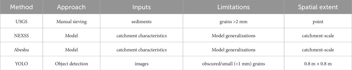
Table 1. comparison of methods used to estimate D50 values for the YRB and methodological characteristics.

2.4 Basin characteristics

To evaluate the relationships between D50 estimates and basin/stream variables, we collected watershed characteristics following methods in Gomez-Velez et al. (2015) and Abeshu et al. (2022). We present variables at two spatial resolutions for each site based on NHDPLUS nomenclature: basin-scale, which represents the total upstream drainage area for each NHD stream reach, and catchment-scale, which represents the smallest NHDPLUS catchment drainage area associated with each NHD stream reach. We selected one land-cover metric (percent urban land cover), two catchment metrics (mean catchment elevation and catchment area), two stream characteristics (total stream length and average stream slope) and two climate parameters (precipitation as snow and potential evapotranspiration) as variables that may relate to the spatial variability of D50 across watersheds.

2.5 Statistics

All spatial and statistical analyses were conducted in R v4.0.5 (R Core Team, 2021). Model performance was assessed by Chen et al. (2024), and presented briefly here for context. Goodness-of-fit using Nash-Sutcliffe (NSE, a measure of goodness-of-fit to a least-squares regression line) in preference to R², as NSE is associated with variance from the 1:1 line rather than variance from a best-fit line (e.g., Regier et al., 2022), was 0.98. We quantified the error associated with YOLO predictions using mean absolute relative error (MARE) normalized to the average D50 value, with a final model MARE of 6.65%. For additional model performance statistics, please refer to Chen et al. (2024). All significance tests were based on a p-value threshold of 0.05. In order to compare the distributions of D50 values to a common reference distribution, we included a distribution of D50 values for sites across the continental United States originally presented in Figure 1D of Abeshu et al. (2022), which we first digitized (https://apps.automeris.io/wpd/), then normalized to a total count of 100 in order to scale to the magnitude of our sample size. Statistical differences between group means were assessed using Wilcoxon tests which are more robust to non-normal distributions than parametric alternatives. Correlations between variables were calculated using Spearman’s rho (r). Prior to correlation calculations, all variables were normalized using the Yeo-Johnson transformation from the bestNormalize R package (Peterson, 2021), which is capable of handling negative values. Spatial analysis to determine straight-line distances between sites, which we selected in preference to flowline distance for simplicity, and the main stem of the Yakima River was conducted using the sf R package (Pebesma, 2018).

3 Results

3.1 Comparison to existing D50 estimates

Figure 2 compares the four methods used to measure or estimate D50 across the YRB (Table 1). We observed significant (p-values <0.05) differences in median D50 values (Figure 2A), with the difference between YOLO and NEXSS being the least significant (p = 0.025), while all remaining comparisons were highly significant (p < 0.0001). YOLO-enabled D50 estimates were highest, followed by the two catchment characteristics-based methods, and USGS D50 measurements having the lowest mean D50 (mean D50 values of 108, 21.4, 1.2, and 0.2 mm, respectively, Table 2). Variance also differed markedly between estimation methods, with standard deviations of 68.4, 26.9, and 0.7, and 0.2 for YOLO, NEXSS, Abeshu, and USGS, respectively (Table 2).

Figure 2

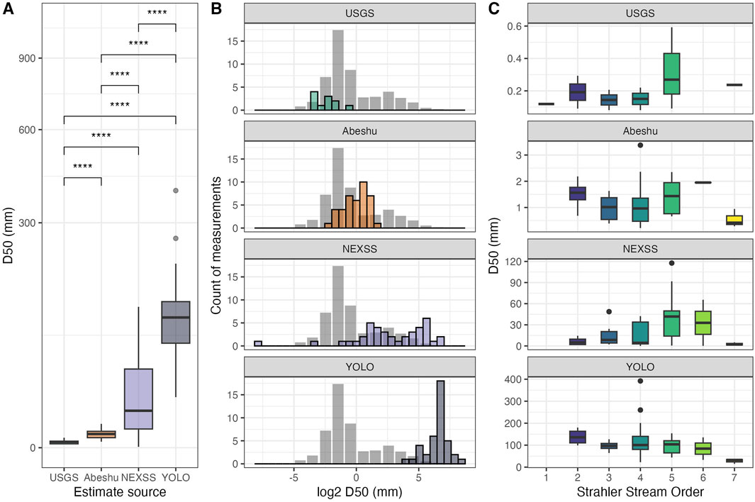
Figure 2. A comparison of D50 estimates across the four methods included in this study (see Table 1 for a summary of these methods). Values are presented as a direct comparison (A) as boxplots, with significant differences shown based on Wilcoxon pairwise tests (**** = p < 0.001), (B) a comparison of distributions for each of the four methods (in color) relative to a standard distribution of D50 measurements (in gray) across the continental US, originally presented in Abeshu et al. (2022), with all values log₂-transformed to improve visualization, and (C) the distribution of D50 estimates across stream orders for each of the four methods. Note: vertical axes are different scales to improve visibility of each dataset. Figure 2C with a common y-axis is presented in Supplementary Figure S2 for reference.

Table 2

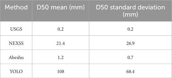
Table 2. summary statistics for the different methods used to estimate D50 values in Table 1.

To better understand how distributions of D50 produced by each estimation method compare, we plotted estimates for the YRB relative to a distribution of D50 values collected from 2,577 stations presented in Abeshu et al. (2022) across the continental US (CONUS) in Figure 2B. We note that while the continental-scale distribution represents a wide range of elevations and gradients, the YRB is composed primarily of high-gradient, high-elevation streams (Supplementary Figure S1). As such, we expected that YRB sites would have larger grains relative to the continental-scale distribution. All methods except USGS skewed to the right relative to the CONUS distribution, while USGS measurements skewed left (Figure 2B). Both Abeshu and YOLO-enabled estimates followed generally unimodal distributions, while USGS estimates did not follow a clear distribution (likely due to limited sample size). NEXSS estimates represented a generally bimodal distribution, with notable outliers at very small D50 values, with a minimum value of 0.005 mm (5 µm), which was well below the lower limit of the CONUS distribution.

We next explored how each method’s estimates changed with stream order (Figure 2C). Based on geomorphology, we expected that lower-order streams would generally have larger grains, and that grain size would generally decrease as stream order increased due to downstream fining (e.g., Menting et al., 2015). Consistent with this theory, the highest stream order corresponded to the lowest D50 values for all methods with the exception of USGS, which showed a general increase in D50 from lowest to highest stream order. However, we only observed consistently monotonic relationships across stream orders 2-6 for YOLO, but not any of the other methods (Figure 2C). For Abeshu, we observe decreasing trends from stream order 2 to stream order 4, then increasing D50 values from stream order 4 to stream order 6. In contrast, NEXSS estimates show increasing D50 values from stream order 2 to 5, and then a decrease from 5 to 6. Similar to Abeshu, USGS D50 values showed a U-shaped pattern from 2nd to 5th order streams (Figure 2C).

3.2 Relationships to basin characteristics

Next, we investigated how the characteristics across the watershed related spatially to D50 values for the four methods included in this study. To understand broad spatial variation with general basin characteristics, we plotted D50 values across the YRB for each D50 source (Figure 3). All methods presented different spatial patterns, which we visualized as above and below median values for simplicity. Higher (above median) Abeshu D50 estimates generally clustered in the northern part of the basin, but also along the Satus tributary in the southwest. Similarly, higher NEXSS D50 values cluster consistently in the northern half of the basin, with highest values clustered along the northernmost tributary sampled. In contrast, YOLO-enabled estimates were spatially distributed, with highest D50 values on tributaries in the middle of the basin. Consistent with Figure 2C, the 7th order site located in the far southeast corner of the basin is below median for both catchment characteristics-based methods and YOLO, but is above median for USGS (Figure 3).

Figure 3

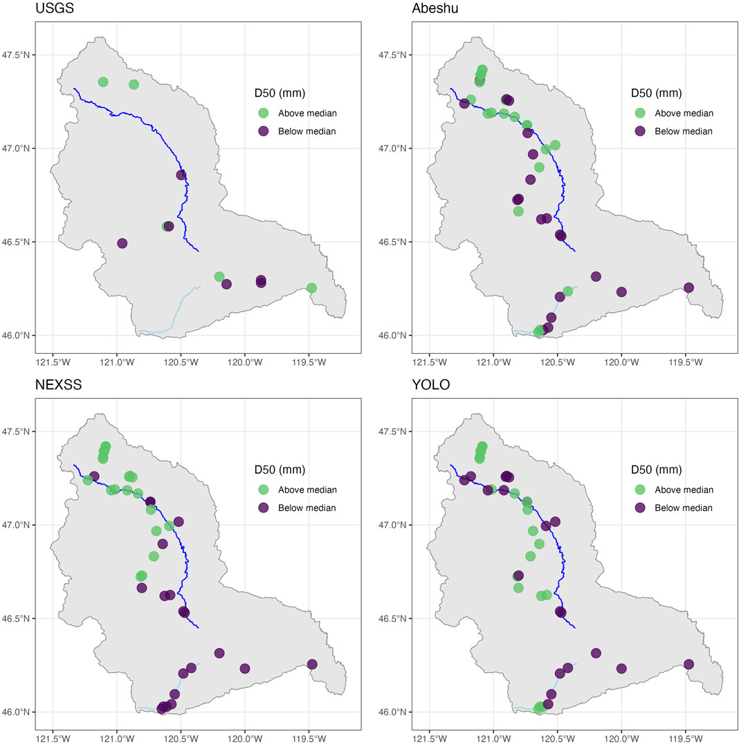
Figure 3. A spatial comparison of D50 values distributed across the YRB for the four methods included in this study (see Table 1 for a summary of these methods). All available USGS sites were used, while only NEXSS and Abeshu estimates matching reaches with YOLO-enabled estimates were included. Note that medians are determined separately for each method. The main stem of the Yakima River is plotted in dark blue, and Satus Creek is plotted in light blue, as spatial references for two waterways referenced in the text.

To quantitatively explore these relationships, we compared differences in latitude, longitude, and straight-line distance from the main stem of the Yakima River for all sites in Figure 3 between above-median and below-median D50 values (Supplementary Figure S3). For distance from the main stem of the Yakima River, YOLO was the only method of the four that showed significant differences (p = 0.03) between above-median and below-median values (Supplementary Figure S3), where above-median D50 sites were considerably farther from the main stem of the Yakima River (median: 15.6 km) compared to below-median D50 sites (median: 1.8 km). For both Abeshu and NEXSS, above-median D50 values were located at more northern latitudes and more western longitudes, while above-median D50 values were located at more western longitudes for YOLO (all p-values <0.05). Neither YOLO nor USGS D50 values showed significant relationships to latitude (Supplementary Figure S3).

To better understand how D50 estimates related to each other and catchment properties, we examined correlations between D50 estimates and basin characteristics (Figure 4). Because the USGS D50 dataset has a much smaller sample size and many sites were not co-located with the other three methods, they were excluded from this analysis. Since we were interested in understanding how the scale of environmental characteristics relates to each D50 estimation method, we separately explored correlations to environmental characteristics computed at the basin-scale (Figure 4A), and the same environmental characteristics, but calculated at catchment resolution (Figure 4B). We note that the basin-scale and catchment-scale are defined in the Methods. Among the three D50 estimation methods, we observed the strongest correlation between Abeshu and NEXSS (r = 0.25), while correlations to YOLO were weaker (r = 0.15 and 0.18 respectively). This is not surprising as Abeshu and NEXSS methods estimated using large-scale modeling approaches (Table 1).

Figure 4

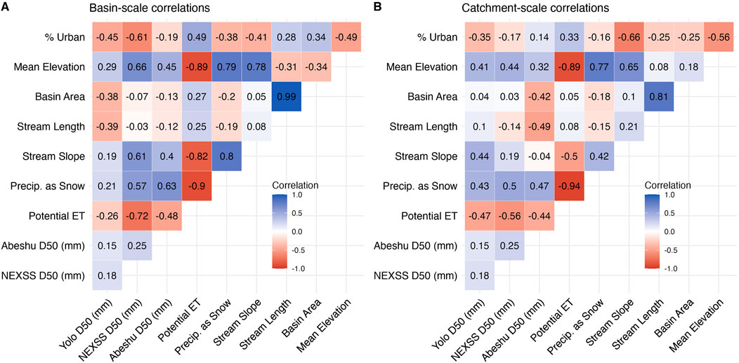
Figure 4. Spearman correlations (presented numerically as numbers and visually as colors) between the three methods with spatially co-located D50 estimates and catchment characteristics (urban = % urban land cover, elev_mean = mean catchment elevation, prsnow = precipitation as snow, and pet = potential evapotranspiration) for (A) basin-scale, and (B) catchment-scale. Prefixes indicate basin-scale (“tot”) or catchment-scale (“cat”) where applicable.

At the basin scale (Figure 4A), NEXSS exhibited the strongest correlation to evapotranspiration (r = 0.72) and strong correlations (r > |0.5|) to all catchment variables except for basin area and stream length. Abeshu correlations were weaker, with the strongest correlation to precipitation as snow (r = 0.63), but generally showed the same patterns (i.e., correlations are positive for both methods or negative for both methods). In contrast, the strongest correlation for YOLO was urban land covert (r = −0.45), and several variables that strongly co-varied with both NEXSS and Abeshu D50 estimates (stream slope, precipitation as snow, elevation, and potential evapotranspiration) showed weaker correlations to YOLO (r < |0.3|). Interestingly, YOLO correlations to basin area and stream length were stronger than those for either Abeshu or NEXSS D50 estimates (Figure 4A).

For catchment-scale characteristics (Figure 4B), the strongest correlations for NEXSS and Abeshu were weaker (r = −0.56 and −0.49, respectively), while the strongest correlation for YOLO was stronger (r = −0.34). Both NEXSS and Abeshu exhibited weaker correlations to all variables except basin area and stream length. We observed the largest decrease in correlation between basin-scale and catchment scale for NEXSS in urban land cover (from r = −0.61 to r = −0.17) and for Abeshu in stream slope (from r = 0.40 to r = −0.04). Strong correlations between NEXSS and precipitation as snow, mean elevation, and evapotranspiration are linked to precipitation and elevation as predictor variables used for D50 estimates (Gomez-Velez et al., 2015). Similar correlations to between Abeshu estimates and snowfall are also expected, as snowfall was identified as a key predictor in their model (Abeshu et al., 2022), and snowfall correlates strongly with both mean elevation and evapotranspiration (Figure 4). For YOLO, correlations to catchment-scale variables were stronger for stream slope, precipitation as snow, and potential evapotranspiration.

3.3 Intra-site variance in YOLO-enabled estimates

To better understand intra-site variability in YOLO D50 estimates, we calculated means and standard deviations for 12 sites with at least 6 images (Figure 5). To directly compare across sites with different numbers of images, we calculated the means and standard deviations for 1,000 random selections of 5 images from each site, and Figure 5 reports the mean of each statistic (mean and standard deviation) across the 1,000 calculations within each site. Standard deviations for each site represent intra-site variability, while standard deviation of all images (“All”) represents inter-site variability within our dataset. For several sites, intra-site variability was larger than inter-site variability (Figure 5A). Because mean values differ widely across the sites in Figure 5A, we normalized standard deviations to mean values to directly compare intra-site and inter-site variability (Figure 5B). Based on this analysis, several sites, most notably S17R, exhibited higher intra-site variability than the inter-site variability within our dataset.

Figure 5

Figure 5. (A) Calculated intra-site variability for all study sites with at least 6 images available. Mean and standard deviation (SD) values for D50 (mm) were calculated as the average of 1,000 subsets of 5 images randomly sampled via bootstrapping from all images available at a given site (or across the full dataset of images estimated by YOLO for “All”), with mean values presented as dots, and upper/lower error bars to represent ± one standard deviation. (B) Calculated coefficients of variance (standard deviations normalized to mean D50 values) within each site grouping in order to compare variability between sites with different mean D50 values.

3.4 YOLO image grading

To assess how useful our manual grading process was (as described in the Methods), we explored the relationship between assessment by the human eye and YOLO’s internal accuracy in Figure 6. We found that images deemed unsuitable for modeling (Image suitability = “no”) had significantly (p < 0.0001) lower accuracy (mean = 65%) relative to images deemed potentially suitable (“maybe”) and suitable (“yes”), with mean accuracies of ∼72% and 73%, respectively. Images graded “maybe” or “yes” did not have significantly different accuracies (p > 0.05).

Figure 6

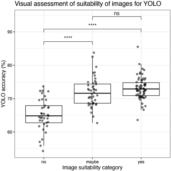
Figure 6. Image suitability was determined for each image, as explained in the methods, and was categorized into “yes”, “no”, or “maybe”. These categories are compared to YOLO’s internally reported accuracy metric for grain identification for each image, with significant differences between categories shown based on Wilcoxon pairwise tests (ns = p > 0.05, **** = p < 0.001).

4 Discussion

4.1 Comparability of object-based and catchment characteristics-based D50 estimates

Our comparison of varying D50 measurement/estimation methods found that each method gave different interpretations of D50 values, their distributions across the study area, and their relationships to basin characteristics. Because the USGS dataset is the only method presented that measures D50 instead of estimating it, we suggest thxat these values represent “ground-truth” for D50 values in the YRB, with caveats that USGS sites are not co-located with YOLO sites, the sample size is limited, and values are constrained by a maximum grain size threshold of 0.2 mm (Table 1). As expected based on minimum grain size (Table 1), mean D50 values were significantly (p < 0.05) higher for the object detection method (YOLO) relative to our understanding of ground-truth (USGS measurements). We expected NEXSS and Abeshu measurements to have similar mean D50 values as USGS because neither catchment characteristics-based method includes a size cut-off (Table 1). However, both methods had significantly (p < 0.0001) higher mean D50 values, indicating that both methods overestimated D50 across the YRB relative to our understanding of ground-truth. Figure 2B indicates some overlap between USGS and Abeshu, and considerably less overlap with NEXSS, indicating that Abeshu estimates are more closely aligned with the true magnitude of D50 across the YRB than YOLO or NEXSS estimates.

NEXSS estimates also had the highest variance across the basin of the three methods (Figure 2A), which is somewhat surprising as we anticipated that catchment characteristics-based estimates would vary less than object detection and manual estimates. In addition, NEXSS estimates are based on a series of empirical relationships, while both Abeshu and YOLO-enabled estimates are derived from machine learning algorithms without explicit boundary conditions, which we anticipated would result in lower variance for NEXSS estimates. Instead, we found that standard deviations were smaller than mean values for both YOLO and Abeshu, but the NEXSS standard deviation was larger than its mean (Figure 2A). We interpret this as NEXSS being more sensitive to a wide range of environmental conditions represented across the YRB relative to Abeshu. Both Abeshu and YOLO methodologies use localized data inputs (relationships based on local basin characteristics and local images, respectively), while NEXSS uses relationships established at a continental scale. In addition, while NEXSS is well-validated in lower-relief catchments (Gomez-Velez et al., 2015), it has been suggested that the methodology may not represent headwater streams accurately (e.g., Ward et al., 2019). Thus, we infer that higher variance from NEXSS estimates is related to a combination of being based on larger scale (and thus less specific) relationships and the prevalence of high-relief locations in this study, for which NEXSS may perform poorly. Our results highlight the benefit of utilizing multiple D50 estimation methods, ideally in concert with manual measurements to ground-truth. For models that depend on D50 to parameterize important basin processes like respiration (Son et al., 2022), based on results in Figure 2, we would expect dramatically different process estimates based on each D50 method, with more variable estimates from YOLO than the other three methods.

We also found differences across estimation methods in the relationships between D50 and stream order (Figure 2C). Based on basin hydrology and geomorphology, we expected that increasing stream order would correlate to lower slope, and therefore decreasing velocities, meaning higher order streams should have smaller D50. While D50 values were generally lowest at the largest stream order, each method exhibited a unique pattern for stream orders 1–6. YOLO clearly followed the expected pattern (Figure 2C). However, the lack of a monotonic decreasing trend is surprising for NEXSS and Abeshu estimates, which are both modeled using catchment properties, and correlate to basin-scale parameters (elevation, stream slope, and precipitation, Figure 4A). Instead, we suggest that deviation from the expected trend can be explained by the complex suite of factors that influence fining across basins, including underlying geology, stream gradient, channel width, and discharge (Church, 2002; Menting et al., 2015). Additionally, these results may suggest localized processes are stronger controls of D50 distributions than general watershed position represented by stream order. note that all methods show increased variance in mid-order streams, which is likely partially due to larger sample sizes, but also may be associated with wider variance in site characteristics for these sites (e.g., Supplementary Figure S1). The lack of a clear trend between D50 and stream order is also consistent with other studies, which found a similar divergence from expected spatial patterns (Menting et al., 2015; Snelder et al., 2011; Splinter et al., 2010), although expected patterns of fining of grains have been observed in lower-relief systems (e.g., Costigan et al., 2014).

Further exploration of the spatial trends in D50 values (Figure 3; Supplementary Figure S3) identified both latitude and longitude as significant covariates for D50 estimates for Abeshu and NEXSS methods, indicating spatially structured controls that may be unrelated to stream order. These results suggest that modeled D50 estimates (Abeshu and NEXSS) follow broader spatial patterns within the basin. Due to lack of relationships to latitude for USGS and YOLO D50 datasets, we suggest these methods may be more sensitive to local controls (Supplementary Figure S3). For YOLO, this is supported by stronger correlations to catchment-scale variables relative to basin-scale variables (Figure 4), and a significant relationship to a site’s distance from the main stem (Supplementary Figure S3). This is consistent with the scales at which the four methods operate, with both Abeshu and NEXSS taking “top-down” views, where D50 estimates are built on continental-scale frameworks which are down-scaled to the site scale and correlate more strongly to larger basin-scale characteristics (Figure 4A). In contrast, the USGS method and YOLO algorithm only access site-specific information, and are therefore unaware of, and theoretically independent of basin properties, although we did observe connections between YOLO and both distance from the main stem (Supplementary Figure S3) and smaller catchment-scale characteristics (Figure 4B).

Together, our results suggest that continental-scale relationships that work for continental-scale modeling of D50 may not be sufficient for modeling at site-to-catchment scales where the generic physical rules do not apply consistently enough to provide trustworthy D50 predictions. As such, methods that incorporate site-scale information (e.g., manual or YOLO) are needed to provide accurate D50 data to hydro-biogeochemical models.

4.2 Advantages of object detection-based D50 estimation

We found YOLO to be an effective method for estimating D50 values for grains larger than pixel resolution (∼1 mm, as reported by the YOLO algorithm for images used in this study), ranging from sand/gravel to cobble (Figure 1). The maximum grain size evaluated here is not tied to YOLO itself, but rather the way in which photos were taken. For example, photos taken from further off the ground (e.g., via drone) could be analyzed by YOLO to capture larger grains (e.g., boulders). Below, we identify some advantages associated with this method, and note that some of these advantages are also shared with other image-based grain size estimation methods (Azarafza et al., 2021; Detert and Weitbrecht, 2020; Lang et al., 2021).

One clear advantage of the YOLO approach is the lack of external data required for D50 estimations. In areas with sparse data coverage (e.g., ungauged catchments), model inputs are based on remotely sensed data with minimal ground-truthing, which can lead to bias and large uncertainty of the input variables (Abeshu et al., 2022; e.g., Gomez-Velez et al., 2015). YOLO stands as a promising complementary method, as stream/river access is not required and results will be as accurate in an ungauged catchment as a heavily instrumented research basin. With advancements in both photography and aerial drone technologies, we see great potential for collecting many images to spatially characterize D50 values across reach-to-basin scales, as explored in other studies (e.g., Lang et al., 2021; Miazza et al., 2024). In addition, the coupling of YOLO with an uncrewed approach could prove a powerful yet safe way to estimate D50 in hard-to-access locations, or during unsafe field conditions. We also see potential for videographic application of the YOLO algorithm, which can process 45–115 frames per second (Redmon et al., 2016), and could therefore potentially provide near real-time D50 estimates. This capability allows for spatially resolved estimates over a short period of time, but also facilitates rapid rescanning of D50 estimates, which could be applicable to collecting high-frequency assessments useful for understanding event-scale (storms, ice-out, etc.) shifts in geomorphology (Lin et al., 2014; Tremblay et al., 2014). In addition, because of the speed with which YOLO processes images, the internal accuracy metric derived for each photo (Figure 6) could be used to assess image suitability for modeling in real-time, allowing operators to adjust the mission (changing altitude, flight paths, etc.) to improve data quality, and potentially indicate when a site has been sufficiently characterized.

Another advantage of YOLO is the ease of collecting large datasets. Unlike manual methods, where each sample requires permission to destructively sample, time in the field to collect, and time in the lab to prepare, analyze, and clean up, the major limitation on the sample size of photos collected for YOLO-enabled estimates is the ability to collect a suitable image. The lack of any disturbance or sample collection requirements for machine-learning object detection approaches bypasses any permitting requirements that other methods that require physical sample collection (e.g., Baptista et al., 2012). Because of this, it is feasible to characterize the average value and variability of D50 at a site simultaneously by collecting multiple images at every site and then calculating D50 values for each image.

The high intra-site variability in Figure 5 highlights the importance of image-based methods for estimating D50 to assess and quantify heterogeneity. To illustrate some sources of high variability, Supplementary Figure S4 presents six images all taken at the same site (S17R), all taken within approximately 100 m of each other on the same river reach, which represent a gradient of GSDs from primarily sand/gravel to boulders that take up almost the entire quadrat. While manual sampling would be capable of collecting multiple samples from a given site, each sample multiples the time, effort, and cost of the dataset collected, and likely limits the number of sites that can be characterized. Conversely, the catchment characteristics-based methods in Table 1 utilize methods that only generate a single estimate for a given reach. By accurately representing this level of intra-site variability, YOLO and other object detection-based methods that can quickly ingest many images, which presents an opportunity to complement manual sampling and catchment characteristics-based modeling estimates. As mentioned above, incorporation of automated image collection via drones or other technologies would extend this capability from a single site to spatially resolved reach-scale profiles, and incorporating edge computing capabilities could provide estimates of data quality and indication of sufficient data collection “on-the-fly”.

4.3 Limitations of object detection estimation

While YOLO provides several advantages, as described above, there are also limitations to this method relative to manual and catchment characteristics-based approaches. First, only surface sediments are captured, while manual methods can characterize sediments at depth. An additional limitation is the method is only as good as the image collected. As an example, Supplementary Figure S5 presents two images where the YOLO algorithm does not capture all grains within the reference frame. On the top row, while most grains are accurately identified, a large grain in the upper left is partially outside the frame and therefore is not identified. The bottom row presents an extreme example of this, where two large grains (boulders) dominate the frame, and neither is identified by the algorithm. For these cases, the YOLO algorithm would need either additional training, flexibility, or potentially manual review after grain assignment to more accurately represent D50 values.

As YOLO is a machine learning object detection algorithm, it is not surprising that visual assessment via the human eye relates to the algorithm’s accuracy (Figure 6). However, the significant distinction between “no” and “maybe”/“yes” highlights the value of this brief visual inspection prior to modeling. Although this quality control pre-processing is a current limitation of the YOLO method, we suggest that future iterations of the YOLO approach could help develop a “living model” that continually learns and improves grain identification by ingesting new images then rerunning. The ability of this living model to automatically detect unsuitable images is supported by the relationships we observed between human-assigned image suitability and machine-assigned YOLO accuracy (Figure 6). Additionally, the iterative retraining of the model with larger and more diverse image datasets would improve the potential transferability of this model to a broader range of fluvial geomorphologies.

Our current approach limits our resolution to ∼1 mm grains and larger, making it useful in gravel/cobble-dominated streams. However, using a higher-resolution imaging system would improve the ability to resolve smaller grains, including sandy substrates. In heterogeneous catchments, we suggest carrying multiple, clearly labeled quadrats as a simple and cheap solution that would likely significantly improve YOLO performance. We also note that, because quadrats are placed manually, utilizing best practices for random sampling (e.g., randomly selecting cells from a grid) is important to protect against sampling bias. The YOLO detection method can underperform in variable lighting conditions, including submerged sediments or exposed sediments interacting with flowing water. Additionally, strong sunlight can wash out images, and low light can lead to blur, both of which degrade YOLO performance. We suggest collecting photos on sunny days when the sun is close to overhead as possible to minimize these potential issues.

Finally, we note that the lack of co-location of USGS sites with YOLO sites complicates direct comparison of these two methods. To better understand this limitation, we compared NEXSS values for all reaches represented in the YOLO dataset to NEXSS values for all reaches represented in the USGS dataset to understand if these sample distributions represent different D50 regimes within the YRB (Supplementary Figure S6). Our comparison indicated that YOLO sites generally had larger NEXSS D50 values compared to NEXSS D50 values at USGS sites, although there was considerable overlap between these datasets (Supplementary Figure S6). While co-location of manual and object detection estimates is beyond the scope of our study, this limits our ability to directly compare manual measurements to our object detection method, and this uncertainty limits the generalizability of our results to other basins. We suggest that future studies should either collect direct manual measurements or attempt to co-locate with a subset of sites that have existing manual measurements to improve cross-method comparisons.

4.4 Future directions

We see great potential for the YOLO algorithm and other object detection methods to be incorporated into a living model that 1) ingests new images supplied via a simple interface (potentially via a publicly available app supporting crowdsourced input), 2) automatically assesses image quality and variability as photos are taken, and 3) reruns the model incorporating the new information. As mentioned above, this opens an opportunity for real-time quality control during data collection in the field, simultaneously improving YOLO model fidelity, optimizing image-capture field efforts (e.g., informing investigators when enough images have been collected to sufficiently represent the study site or system), and eliminating the need to manually assess image quality prior to modeling. This edge computing approach to data-model integration would ensure that high-quality data are collected for all sites via real-time quality control, eliminating site loss due to image issues, which was a limiting factor to the accuracy of the YOLO model in this study (Figure 6). Coupled with technologies for imaging large spatial scales like drones, a living YOLO model could rapidly expand from site to catchment and basin-scale D50 estimates.

Because of the ability of YOLO to quickly estimate D50 from images, we suggest that YOLO holds potential to improve spatiotemporally resolved D50 estimates in combination with site-specific (manual) and over-generalized catchment characteristics-based approaches. As an example, in the YRB, manual D50 estimates are available, but at a limited number of locations and over limited time-scales that make extrapolation difficult. Likewise, as discussed above, catchment characteristics-based estimates can be down-scaled to individual reaches, but are over-generalized due to the coarser resolution of their input parameters and can be biased by basin features (e.g., a model parameterized in low-relief systems exhibits high variability in our high-relief basin). Our YOLO-enabled estimates provide site-specific information at a larger number of sites than the manual estimations, but are not biased by model constraints or input parameter resolution. As such, exploring the differences and similarities between 1) YOLO and co-located or co-collected manual measurements, and 2) YOLO and catchment characteristics-based measurements could provide basin-specific calibration of models capable of reconciling the accuracy of direct measurements with the spatiotemporal resolution of catchment characteristics-based estimates. While these relationships would be basin-specific, additional YOLO campaigns in other, contrasting basins with manual and catchment characteristics-based estimates would move towards basin-agnostic relationships.

YOLO-enabled estimates across multiple basins, incorporated into an iterative, living model could then be scaled up to provide continuous spatial coverage of D50 estimates required to parameterize basin-scale model data needs. We see potential for such an approach, utilized within a data-model feedback loop like the Model-Experiment (ModEx) framework (Serbin et al., 2021) to iteratively identify locations of high uncertainty for D50 estimates across a region of interest, which can help target data collection for improving YOLO models. In turn, because hydro-biogeochemical models depend on D50 for parameterization, iterative improvement of D50 products would iteratively improve model performance, better constraining estimates of key basin functions like sediment respiration (Son et al., 2022).

Finally, we recognize that there are many emerging machine-learning enabled technologies relevant to estimation of D50. Each of these methods represents substantial improvements over traditional techniques in terms of throughput, and has trade-offs with our YOLO-enabled method in processing speed, simplicity of implementation, and accuracy (Detert and Weitbrecht, 2020; Miazza et al., 2024). For instance, GRAINet uses convolutional neural networks (CNNs) and a two-stage architecture that segments images then classifies individual grains, which provides high precision but requires greater compute resources relative to our YOLO approach (Lang et al., 2021). Similarly, the method described by Mair et al. (2024) utilizes CNNs to efficiently estimate grain sizes across a broader range of image types. SediNet is another alternative that can estimate equivalent sieve diameters directly from images (Buscombe, 2020). We encourage future efforts that compare YOLO-enabled D50 estimation with methods used in other recent publications such as those listed above.

5 Conclusion

In this study, we explored how estimates of median GSD (D50) derived from four different methods varied across the Yakima River Basin. Object detection methods (including the YOLO approach in this study) bring advantages of rapid throughput, low sample cost, and site-specific information, which complement both manual and catchment characteristics-based methods, which are limited by low throughput and over-generalization, respectively. In addition, imaged-based methods like YOLO can easily estimate intra-site variance, which is difficult with manual methods, and not possible for the catchment characteristics-based methods explored here. As such, we suggest that object detection methods can complement site-specific manual measurements and “top-down” catchment characteristics-based estimates towards spatially and temporally resolved, scalable estimates of GSD (both median and variance). The flexibility of the data input (images of sufficient quality with some physical reference) and the speed of the YOLO method are primed for use on uncrewed platforms, inclusion in citizen or crowdsourced science campaigns, and ingestion of existing high-resolution datasets to rapidly improve the coverage and resolution of ground-truthed GSD estimates from reach to continental scales. We also discuss several limitations associated with this method, including lack of depth-resolved estimates. We envision this coalescence of data as a living model that maintains site-specific accuracy while scaling predictive capabilities up to regional or continental scales as more data from an increasingly broad range of ecosystem types and geographic regions are ingested. Using this constantly improving D50 product, in concert with manual and catchment characteristics-based D50 values, we see strong potential to iteratively improve D50 representation in models improving both quantitative (magnitude) and qualitative (spatial and temporal organization) estimates of basin-scale hydro-biogeochemical processes.

Data availability statement

Publicly available datasets were analyzed in this study. These data can be found here: https://data.ess-dive.lbl.gov/view/doi%3A10.15485%2F1972232.

Author contributions

PR: Conceptualization, Data curation, Formal Analysis, Investigation, Methodology, Project administration, Resources, Software, Supervision, Validation, Visualization, Writing – original draft, Writing – review and editing. YC: Conceptualization, Data curation, Formal Analysis, Investigation, Methodology, Software, Validation, Writing – original draft, Writing – review and editing. KS: Data curation, Formal Analysis, Investigation, Software, Validation, Writing – original draft, Writing – review and editing. JB: Data curation, Formal Analysis, Software, Validation, Writing – review and editing. BF: Data curation, Writing – review and editing. AG: Data curation, Writing – review and editing. MK: Data curation, Writing – review and editing. KR: Validation, Writing – review and editing. JS: Conceptualization, Funding acquisition, Project administration, Resources, Writing – review and editing.

Funding

The author(s) declare that financial support was received for the research and/or publication of this article. This research was supported by the U.S. Department of Energy (DOE), Office of Biological and Environmental Research (BER), Environmental System Science (ESS) Program as part of the River Corridor Science Focus Area (SFA) at the Pacific Northwest National Laboratory (PNNL). PNNL is operated by Battelle Memorial Institute for the DOE under Contract No. DE-AC05-76RL01830.

Acknowledgments

We gratefully acknowledge members of the larger River Corridor Science Focus Area team who collected the field images used for modeling, including Morgan Barnes, Mikayla Borton, Stephanie Fulton, Samantha Grieger, Sophia McKever, Opal Otenburg, Lupita Renteria, and Joshua Torgeson.

Conflict of interest

The authors declare that the research was conducted in the absence of any commercial or financial relationships that could be construed as a potential conflict of interest.

Generative AI statement

The author(s) declare that no Generative AI was used in the creation of this manuscript.

Publisher’s note

All claims expressed in this article are solely those of the authors and do not necessarily represent those of their affiliated organizations, or those of the publisher, the editors and the reviewers. Any product that may be evaluated in this article, or claim that may be made by its manufacturer, is not guaranteed or endorsed by the publisher.

Supplementary material

The Supplementary Material for this article can be found online at: https://www.frontiersin.org/articles/10.3389/feart.2025.1529503/full#supplementary-material

References

Abeshu, G. W., Li, H.-Y., Zhu, Z., Tan, Z., and Leung, L. R. (2022). Median bed-material sediment particle size across rivers in the contiguous US. Earth Syst. Sci. Data 14 (2), 929–942. doi:10.5194/essd-14-929-2022

CrossRef Full Text | Google Scholar

Azarafza, M., Nanehkaran, Y. A., Akgün, H., and Mao, Y. (2021). Application of an image processing-based algorithm for river-side granular sediment gradation distribution analysis. Adv. Mater. Res. 10 (3), 229–244. doi:10.12989/amr.2021.10.3.229

CrossRef Full Text | Google Scholar

Baptista, P., Cunha, T. R., Gama, C., and Bernardes, C. (2012). A new and practical method to obtain grain size measurements in sandy shores based on digital image acquisition and processing. Sediment. Geol. 282, 294–306. doi:10.1016/j.sedgeo.2012.10.005

CrossRef Full Text | Google Scholar

Buscombe, D. (2020). SediNet: a configurable deep learning model for mixed qualitative and quantitative optical granulometry. Earth Surf. Process. Landforms 45 (3), 638–651. doi:10.1002/esp.4760

CrossRef Full Text | Google Scholar

Buser-Young, J. Z., Garcia, P. E., Schrenk, M. O., Regier, P. J., Ward, N. D., Biçe, K., et al. (2023). Determining the biogeochemical transformations of organic matter composition in rivers using molecular signatures. Front. Water 5. doi:10.3389/frwa.2023.1005792

CrossRef Full Text | Google Scholar

Chang, F.-J., and Chung, C.-H. (2012). Estimation of riverbed grain-size distribution using image-processing techniques. J. Hydrology 440–441, 102–112. doi:10.1016/j.jhydrol.2012.03.032

CrossRef Full Text | Google Scholar

Chen, X., Hassan, M. A., and Fu, X. (2022). Convolutional neural networks for image-based sediment detection applied to a large terrestrial and airborne dataset. Earth Surf. Dyn. 10 (2), 349–366. doi:10.5194/esurf-10-349-2022

CrossRef Full Text | Google Scholar

Chen, Y., Bao, J., Chen, R., Li, B., Yang, Y., Renteria, L., et al. (2024). Quantifying streambed grain size, uncertainty, and hydrobiogeochemical parameters using machine learning model YOLO. Water Resour. Res. 60 (11), e2023WR036456. doi:10.1029/2023WR036456

CrossRef Full Text | Google Scholar

Church, M. (2002). Geomorphic thresholds in riverine landscapes. Freshw. Biol. 47 (4), 541–557. doi:10.1046/j.1365-2427.2002.00919.x

CrossRef Full Text | Google Scholar

Costigan, K. H., Daniels, M. D., Perkin, J. S., and Gido, K. B. (2014). Longitudinal variability in hydraulic geometry and substrate characteristics of a Great Plains sand-bed river. Geomorphology 210, 48–58. doi:10.1016/j.geomorph.2013.12.017

CrossRef Full Text | Google Scholar

De Cicco, L. A., Hirsch, R. M., Lorenz, D., and Watkins, D. (2018). dataRetrieval. U.S. Geol. Surv. doi:10.5066/P9X4L3GE

CrossRef Full Text | Google Scholar

Detert, M., and Weitbrecht, V. (2012). Automatic object detection to analyze the geometry of gravel grains - a free stand-alone tool. River Flow 2012 - Proc. Int. Conf. Fluvial Hydraulics 1, 595–600 (London, United Kingdom). Available at: https://www.routledge.com/River-Flow-2012/MurilloMunoz/p/book/9780415621298?srsltid=AfmBOoo7XNQUCdzHLLgY4YN04pcqPPcJNMrU49uIhC15zIVFSiKV-kui.pdf

Google Scholar

Detert, V., and Weitbrecht, M. (2020). “Determining image-based grain size distribution with suboptimal conditioned photos,” in River flow 2020 (CRC Press).

Google Scholar

Faustini, J. M., and Kaufmann, P. R. (2007). Adequacy of visually classified particle count statistics from regional stream habitat Surveys1. JAWRA J. Am. Water Resour. Assoc. 43 (5), 1293–1315. doi:10.1111/j.1752-1688.2007.00114.x

CrossRef Full Text | Google Scholar

Folk, R. L. (1966). A review of grain-size parameters. Sedimentology 6 (2), 73–93. doi:10.1111/j.1365-3091.1966.tb01572.x

CrossRef Full Text | Google Scholar

Fulton, S. G., Barnes, M., Borton, M. A., Chen, X., Farris, Y., Forbes, B., et al. (2022). Spatial study 2021: sensor-based time series of surface water temperature, specific conductance, total dissolved solids, turbidity, pH, and dissolved oxygen from across multiple watersheds in the Yakima River Basin. ESS-DIVE. doi:10.15485/1892052

CrossRef Full Text | Google Scholar

Gaines, R., and Priestas, A. (2016). Particle size distributions of bed sediments along the Mississippi river, grafton, Illinois to head of passes. USACE. doi:10.13140/RG.2.1.2492.1207

CrossRef Full Text | Google Scholar

Glaser, C., Zarfl, C., Rügner, H., Lewis, A., and Schwientek, M. (2020). Analyzing particle-associated pollutant transport to identify in-stream sediment processes during a high flow event. Water 12 (6), 1794. doi:10.3390/w12061794

CrossRef Full Text | Google Scholar

Gomez-Velez, J. D., and Harvey, J. W. (2014). A hydrogeomorphic river network model predicts where and why hyporheic exchange is important in large basins. Geophys. Res. Lett. 41 (18), 6403–6412. doi:10.1002/2014GL061099

CrossRef Full Text | Google Scholar

Gomez-Velez, J. D., Harvey, J. W., Cardenas, M. B., and Kiel, B. (2015). Denitrification in the Mississippi River network controlled by flow through river bedforms. Nat. Geosci. 8 (12), 941–945. doi:10.1038/ngeo2567

CrossRef Full Text | Google Scholar

Guy, H. (1969). Laboratory theory and methods for sediment analysis. Tech. Water-Resources Investigations. doi:10.3133/twri05C1

CrossRef Full Text | Google Scholar

Harvey, B. N., Johnson, M. L., Kiernan, J. D., and Green, P. G. (2011). Net dissolved inorganic nitrogen production in hyporheic mesocosms with contrasting sediment size distributions. Hydrobiologia 658 (1), 343–352. doi:10.1007/s10750-010-0504-4

CrossRef Full Text | Google Scholar

He, K., Zhang, X., Ren, S., and Sun, J. (2014). Spatial pyramid pooling in deep convolutional networks for visual recognition. 8691 346–361. doi:10.1007/978-3-319-10578-9_23

CrossRef Full Text | Google Scholar

Lang, N., Irniger, A., Rozniak, A., Hunziker, R., Wegner, J. D., and Schindler, K. (2021). GRAINet: mapping grain size distributions in river beds from UAV images with convolutional neural networks. Hydrology Earth Syst. Sci. 25 (5), 2567–2597. doi:10.5194/hess-25-2567-2021

CrossRef Full Text | Google Scholar

Lepesqueur, J., Hostache, R., Martínez-Carreras, N., Montargès-Pelletier, E., and Hissler, C. (2019). Sediment transport modelling in riverine environments: on the importance of grain-size distribution, sediment density, and suspended sediment concentrations at the upstream boundary. Hydrology Earth Syst. Sci. 23 (9), 3901–3915. doi:10.5194/hess-23-3901-2019

CrossRef Full Text | Google Scholar

Lin, C.-P., Wang, Y.-M., Tfwala, S. S., and Chen, C.-N. (2014). The variation of riverbed material due to tropical storms in shi-wen river, taiwan. Sci. World J. 2014, 1–12. doi:10.1155/2014/580936

PubMed Abstract | CrossRef Full Text | Google Scholar

Lopez-Garcia, P., Muñoz-Perez, J. J., Contreras, A., Vidal, J., Jigena, B., Santos, J. J., et al. (2021). Error on the estimation of sand size parameters when using small diameter sieves and a solution. Front. Mar. Sci. 8. doi:10.3389/fmars.2021.738479

CrossRef Full Text | Google Scholar

Mair, D., Witz, G., Do Prado, A. H., Garefalakis, P., and Schlunegger, F. (2024). Automated detecting, segmenting and measuring of grains in images of fluvial sediments: the potential for large and precise data from specialist deep learning models and transfer learning. Earth Surf. Process. Landforms 49 (3), 1099–1116. doi:10.1002/esp.5755

CrossRef Full Text | Google Scholar

Menting, F., Langston, A. L., and Temme, A. J. A. M. (2015). Downstream fining, selective transport, and hillslope influence on channel bed sediment in mountain streams, Colorado Front Range, USA. Geomorphology 239, 91–105. doi:10.1016/j.geomorph.2015.03.018

CrossRef Full Text | Google Scholar

Miazza, R., Pascal, I., and Ancey, C. (2024). Automated grain sizing from uncrewed aerial vehicles imagery of a gravel-bed river: benchmarking of three object-based methods. Earth Surf. Process. Landforms 49 (5), 1503–1514. doi:10.1002/esp.5782

CrossRef Full Text | Google Scholar

Mori, N., Debeljak, B., Kocman, D., and Simčič, T. (2017). Testing the influence of sediment granulometry on heterotrophic respiration with a new laboratory flow-through system. J. Soils Sediments 17 (7), 1939–1947. doi:10.1007/s11368-016-1613-0

CrossRef Full Text | Google Scholar

Pebesma, E. (2018). Simple features for R: standardized support for spatial vector data. R J. 10 (1), 439–446. doi:10.32614/rj-2018-009

CrossRef Full Text | Google Scholar

Peterson, R. A. (2021). Finding optimal normalizing transformations via bestNormalize. R J. 13 (1), 310–329. doi:10.32614/rj-2021-041

CrossRef Full Text | Google Scholar

Poullet, P., Muñoz-Perez, J. J., Lopez, P., García-Lopez, S., Martell, R., Silva, R., et al. (2019). Sand size variability inside the hopper of a trailing suction dredger for beach nourishment purposes. Geo-Marine Lett. 39 (6), 513–520. doi:10.1007/s00367-019-00615-w

CrossRef Full Text | Google Scholar

Purinton, B., and Bookhagen, B. (2019). Introducing PebbleCounts: a grain-sizing tool for photo surveys of dynamic gravel-bed rivers. Earth Surf. Dyn. 7 (3), 859–877. doi:10.5194/esurf-7-859-2019

CrossRef Full Text | Google Scholar

R Core Team (2021). R: a language and environment for statistical computing. Vienna, Austria.

Google Scholar

Redmon, J., Divvala, S., Girshick, R., and Farhadi, A. (2016). You only Look once: unified, real-time object detection. arXiv. doi:10.48550/arXiv.1506.02640

CrossRef Full Text | Google Scholar

Regier, P., Chen, Y., Son, K., Bao, J., Forbes, B., Goldman, A. E., et al. (2023). Data associated with “Machine learning photogrammetric analysis of images provides a scalable approach to study riverbed grain size distributions”. ESS-DIVE. Available online at: https://data.ess-dive.lbl.gov/view/doi%3A10.15485%2F1972232.

Google Scholar

Regier, P., Duggan, M., Myers-Pigg, A., and Ward, N. (2022). Effects of random forest modeling decisions on biogeochemical time series predictions. Limnol. Oceanogr. Methods 21, 40–52. doi:10.1002/lom3.10523

CrossRef Full Text | Google Scholar

Ren, H., Hou, Z., Duan, Z., Song, X., Perkins, W. A., Richmond, M. C., et al. (2020). Spatial mapping of riverbed grain-size distribution using machine learning. Front. Water 2. doi:10.3389/frwa.2020.551627

CrossRef Full Text | Google Scholar

Rickenmann, D., and Recking, A. (2011). Evaluation of flow resistance in gravel-bed rivers through a large field data set. Water Resour. Res. 47 (7). doi:10.1029/2010WR009793

CrossRef Full Text | Google Scholar

Schwarz, G. E., Jackson, S. E., and Wieczorek, M. E. (2018). Select attributes for NHDPlus version 2.1 reach catchments and modified network routed upstream watersheds for the conterminous United States. U.S. Geol. Surv. doi:10.5066/F7765D7V

CrossRef Full Text | Google Scholar

Serbin, S. P., Giangrande, S. E., Kuang, C., Urban, N., and Pouchard, L. (2021). AI to automate modEx for optimal predictive Improvement and scientific discovery (No. AI4ESP-1119). Artif. Intell. Earth Syst. Predict. (AI4ESP) Collab. (United States). doi:10.2172/1769662

CrossRef Full Text | Google Scholar

Snelder, T. H., Lamouroux, N., and Pella, H. (2011). Empirical modelling of large scale patterns in river bed surface grain size. Geomorphology 127 (3), 189–197. doi:10.1016/j.geomorph.2010.12.015

CrossRef Full Text | Google Scholar

Son, K., Fang, Y., Gomez-Velez, J. D., and Chen, X. (2022). Spatial microbial respiration variations in the hyporheic zones within the Columbia River Basin. J. Geophys. Res. Biogeosciences 127, e2021JG006654. doi:10.1029/2021JG006654

CrossRef Full Text | Google Scholar

Splinter, D. K., Dauwalter, D. C., Marston, R. A., and Fisher, W. L. (2010). Ecoregions and stream morphology in eastern Oklahoma. Geomorphology 122 (1), 117–128. doi:10.1016/j.geomorph.2010.06.004

CrossRef Full Text | Google Scholar

Stähly, S., Friedrich, H., and Detert, M. (2017). Size ratio of fluvial grains’ intermediate axes assessed by image processing and square-hole sieving. J. Hydraulic Eng. 143 (6), 06017005. doi:10.1061/(ASCE)HY.1943-7900.0001286

CrossRef Full Text | Google Scholar

Steer, P., Guerit, L., Lague, D., Crave, A., and Gourdon, A. (2022). Size, shape and orientation matter: fast and semi-automatic measurement of grain geometries from 3D point clouds. Earth Surface Dynamics, 10 (6),1211–1232. doi:10.5194/esurf-10-1211-2022

CrossRef Full Text | Google Scholar

Strahler, A. (1964). “Quantitative geomorphology of drainage basin and channel networks,” in Handbook of applied hydrology, 439–476.

Google Scholar

Stroud Water Research Center (2023). Model my watershed. Available online at: https://wikiwatershed.org.

Google Scholar

Tremblay, P., Leconte, R., Jay Lacey, R. W., and Bergeron, N. (2014). Multi-day anchor ice cycles and bedload transport in a gravel-bed stream. J. Hydrology 519, 364–375. doi:10.1016/j.jhydrol.2014.06.036

CrossRef Full Text | Google Scholar

Vano, J. A., Scott, M. J., Voisin, N., Stöckle, C. O., Hamlet, A. F., Mickelson, K. E. B., et al. (2010). Climate change impacts on water management and irrigated agriculture in the Yakima River Basin, Washington, USA. Clim. Change 102 (1), 287–317. doi:10.1007/s10584-010-9856-z

CrossRef Full Text | Google Scholar

Wang, C.-Y., Liao, H.-Y. M., Yeh, I.-H., Wu, Y.-H., Chen, P.-Y., and Hsieh, J.-W. (2019). CSPNet: a new backbone that can enhance learning capability of CNN. arXiv. doi:10.48550/arXiv.1911.11929

CrossRef Full Text | Google Scholar

Wang, J.-P., François, B., and Lambert, P. (2017). Equations for hydraulic conductivity estimation from particle size distribution: a dimensional analysis. Water Resour. Res. 53 (9), 8127–8134. doi:10.1002/2017WR020888

CrossRef Full Text | Google Scholar

Ward, A. S., Wondzell, S. M., Schmadel, N. M., Herzog, S., Zarnetske, J. P., Baranov, V., et al. (2019). Spatial and temporal variation in river corridor exchange across a 5th-order mountain stream network. Hydrology Earth Syst. Sci. 23 (12), 5199–5225. doi:10.5194/hess-23-5199-2019

CrossRef Full Text | Google Scholar

Wolman, M. (1954). A method of sampling coarse river-bed material. Eos, Trans. Am. Geophys. Union 35 (6), 951–956. doi:10.1029/TR035i006p00951

CrossRef Full Text | Google Scholar

Xia, X., Jia, Z., Liu, T., Zhang, S., and Zhang, L. (2017). Coupled nitrification-denitrification caused by suspended sediment (SPS) in rivers: importance of SPS size and composition. Environ. Sci. and Technol. 51 (1), 212–221. doi:10.1021/acs.est.6b03886

PubMed Abstract | CrossRef Full Text | Google Scholar

Zhang, W., Itoh, K., Tanida, J., and Ichioka, Y. (1990). Parallel distributed processing model with local space-invariant interconnections and its optical architecture. Appl. Opt. 29 (32), 4790–4797. doi:10.1364/AO.29.004790

PubMed Abstract | CrossRef Full Text | Google Scholar