GEOCLASS-image – a versatile machine learning environment for ice-surface classification from high-resolution image data

GEOCLASS-image is an open source cyberinfrastructure (CI) for automated classification of spatial surface structures based on high-resolution image data, consisting of a data-driven and physically informed neural network (NN) system and a data analysis tool for, currently, submeter resolution satellite image data (Maxar WorldView data). The objective of this paper is to introduce GEOCLASS-image v2.0, which provides a solution for two important problems in machine learning in the geosciences: (1) Version 2.0 presents an approach for creating, exporting and sharing labeled training datasets for cryospheric classification tasks for which such datasets do not currently exist. GEOCLASS-image (v2.0) offers options for user-friendly, system-immanent application using a graphical user interface (GUI), and additionally for importing and exporting data sets to facilitate interoperability with other software, a key for advancing Open Science. (2) Combining the advantages of a purely data-driven convolutional NN and a physically driven NN, a new combined NN architecture, termed VarioNet, is derived using a weighted fusion approach that includes one or several additional blocks. The GEOCLASS-image CI, demonstrated here for classification of 11 different glacier surface types which include crevasse classes and water-based classes, extracted from Maxar WorldView1 and WorldView2 data, is expected to generalize to similar classification problems in other geoscience disciplines and any high-resolution satellite imagery.

1 Introduction

The objective of this paper is to describe the capabilities and uses of the GEOCLASS-image cyberinfrastructure (CI), a machine-learning (ML) system that facilitates automated classification of spatial surface structures based in high-resolution image data (Herzfeld et al., 2023). GEOCLASS-image is a data-driven and physically constrained neural network (NN) system, designed to integrate knowledge in physical sciences and computer sciences, rather than relying primarily on computer sciences as the domain for development of ML approaches (Herzfeld et al., 2024). Application of GEOCLASS-image allows to derive physical process understanding from signatures of physical processes that are recorded in high-resolution satellite imagery. Results include parameterized information in the form of thematic maps (time series of segmented satellite imagery) that can be used for geophysical interpretation or to inform numerical modeling. With an easily usable graphical interface and the option to load high-resolution image data from satellites and other sources, GEOCLASS-image meets a need in the cryospheric sciences community for a versatile classification system whose application does not require understanding of computational principles. Here, we describe GEOCLASS-image (v2.0) CI (Herzfeld et al., 2025), an advancement of the open-source GEOCLASS-image (v1.0) CI (Herzfeld et al., 2023) and its importance to the geoscientific community.

The GEOCLASS-image CI is situated in the intersection of (1) geosciences, specifically, glaciology, (2) remote-sensing image classification and (3) development of ML systems, specifically, neural networks. The wide acceptance of Convolutional Neural Networks (CNNs) (Deng et al., 2009; Krizhevsky et al., 2012; Lin et al., 2013; Simonyan and Zisserman, 2014; Tai et al., 2015; He et al., 2016a; b; Huang et al., 2017; Xiang et al., 2018; Song et al., 2019; He et al., 2021; Camps-Valls et al., 2021) may create the perception that CNNs make any other of NNs superfluous. In geoscience applications, this is not the case. De facto, there is a need for physically driven NNs, which allow the incorporation of the geoscientist’s understanding of those spatial processes that drive the expected outcome of a NN.

1.1 The glaciological problem

In order to motivate the need for a data-driven, physically informed approach to ML in the geosciences, we introduce the glaciological problem that will be utilized for the development and evaluation of our classification approach. The ML approach described in this paper is derived using the case study of an Arctic glacier system during surge, the Negribreen Glacier System (NGS) in Svalbard as seen in Figure 1. The NGS is a complex Arctic surge-type glacier that started accelerating in 2016 for the first time in over 80 years and continues to surge at present (2025) (Herzfeld et al., 2021; Trantow and Herzfeld, 2024b; Lefauconnier and Hagen, 1991). A surge is an acceleration of a glacier or glacier system to 10–200 times (200 for the NGS) its normal, quiescent-time velocities. In general, surge-type glaciers flow in quasi-cycles, where long periods of normal flow (quiescent phases) are interspersed with short surge phases of rapid acceleration, wide-spread surface deformation and large-scale mass transfer throughout the glacial system (Harrison and Post, 2003; Jiskoot, 2011; Trantow and Herzfeld, 2024a).

Figure 1

Figure 1. Map of the Negribreen Glacier System (NGS), Svalbard. Region of interest outlined by polygon. Background image: Landsat-8 RGB image acquired 5 August 2019. Inset: Location of the NGS in the Arctic archipelago of Svalbard.

Figure 2 provides exemplary aerial imagery of the structural deformations observed in the NGS in July 2017 when ice-surface speeds were highest. For a marine-terminating glacier system like the NGS, the mass transfer throughout the glacier system results in rapid calving of the heavily crevassed ice and thus mass transfer from the glacier system into the Arctic Ocean. Mass transfer during the height of the acceleration phase in summer 2017 accounted for around one percent of global sea rise in just 3 months (Herzfeld et al., 2021; Trantow and Herzfeld, 2024b; Herzfeld et al., 2024).

Figure 2

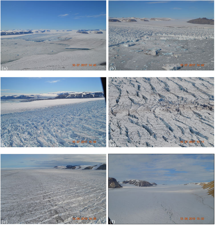
Figure 2. Negribreen Glacier System during surge, overview and surface structures. Aerial photographs collected during the 2017 airborne geophysical observation and ICESat-2 validation campaign over the NGS Negribreen campaign (Geomathematics, Remote Sensing and Cryospheric Sciences Laboratory, University of Colorado Boulder). Photographs by U. Herzfeld and T. Trantow (Flight 2, 2017–07–15) (Herzfeld and Trantow, 2021). (a) Overview of the NGS during the acceleration phase of the surge in July 2017. The heavily crevassed surface of the surging Negribreen (background) contrasts the smooth surface of slow-moving Ordonnansbreen (foreground and background right). Surface melt streams are visible on the Ordonnansbreen ice surface indicated as darker features in the foreground of the photograph. (b) Calving front of Negribreen, where heavily crevassed ice advances into the Arctic sea. Ordnonnansbreen in background. (c) Heavy crevassing caused by the surge in the foreground, with minimal or no crevassing in the background (lower Negribreen). (d) Shear crevasses caused by the surge (Negribreen). (e) Fields of parallel crevasses formed by the surge (upper Negribreen). (f) Surface melt stream on non-surging Ordnonnansbreen (view upglacier).

The complicated and hazardous nature of surging glacier systems calls for the need to fully understand the physical processes that occur during a surge at various spatiotemporal resolutions, which requires a large and comprehensive database and in turn, the infrastructure to efficiently analyze these data. In this paper, we demonstrate the capability of GEOCLASS-image to extract information on the acceleration phase of the NGS by classifying surface crevasses and melt captured in high-resolution satellite imagery. Crevasses of different types form as the surge progresses, which reflect the dynamic forces the ice experiences (Herzfeld and Zahner, 2001; Herzfeld et al., 2013). The complexity of this problem illustrates that geophysical knowledge is required to effectively design and evaluate a ML system for understanding the physical processes involved in the surge phenomenon.

In turn, the multitude of many different ice-surface types that occur in close proximity as a consequence of the rapid transformation of the glacier surface during surge makes the NGS an ideal testbed for development of an advanced ML approach that combines the advantages of a physically constrained NN and a data-driven CNN. The resultant NN, developed and trained for the NGS, can be expected to generalize to many other types of Arctic and subArctic glacier systems, such as those in Greenland, Alaska and the Canadian Archipelago.

1.2 Image classification

In addition to physical knowledge, large amounts of data are needed to extract the complex information described in the glaciological problem section, and the data needs to effectively capture the relevant processes under investigation. In contrast, advance of NNs, specifically CNNs, has been supported by and measured against a relatively small collection of published bench-mark data sets (He et al., 2016a; b; Song et al., 2019). As they are unrelated to geosciences, these data sets are not useful to advance knowledge in the geosciences. Development of the GEOCLASS-image CI has relied on utilization of Maxar WorldView image data (Herzfeld et al., 2024). Generalization to facilitate use of other data sets is one of the objectives of the software described here.

1.3 NNs in the geosciences

A review of NNs, especially in the geosciences and in (satellite) image classification is given in (Herzfeld et al., 2024). An under-researched problem in NN development is the creation of labeled training data sets (Meyer and Pebesma, 2021) of sufficient quality and size to allow training of deep networks, such as CNNs with many layers (Goodfellow et al., 2016; Song et al., 2019; Herzfeld et al., 2024). To address this gap, GEOCLASS-image includes a module for labeling training data and an approach for increasing the size of such training data sets through a combination of expert knowledge and NN action (Herzfeld et al., 2024). In GEOCLASS-image (v2.0), additional options to further increase versatility in labeling and training are realized. Other challenges associated with advancing remote-sensing-data classification, especially in the Earth sciences, identified in the literature (e.g.,.Song et al. (2019); Meyer and Pebesma (2021); Virts et al. (2020); Liu et al. (2020), include a need for development of image-classification-problem-specific CNN architectures and time-efficiency of training CNNs for image classification. GEOCLASS-image (v2.0) addresses all three. In this paper, we build on approaches described in (Herzfeld et al., 2024), such as using a shallow, physically driven network to increase training image quantity, to then drive the training of a deep network, and present alternatives to this approach. Here, we will introduce a new, combined NN model (VarioNet) that integrates a geostatistically-informed multi-layer perceptron (VarioMLP) (Herzfeld and Zahner, 2001) and a relatively shallow CNN (ResNet-18) (He et al., 2016a). ResNets are a family of so-called residual networks with depths of up to 1,001 layers (He et al., 2016a; b, 2021), of which ResNet-18 is the one with the least number of layers. In GEOCLASS-image, we use a form of ResNet, because ResNets have been found to excel at image classification problems and ResNet-18 is sufficient for the task at hand (Herzfeld et al., 2024).

To facilitate open science, we include a summarized user guide for the GEOCLASS-image (v2.0) CI, including software download, data set labeling, training and NN model derivation and application.

2 Approach

2.1 Overview of GEOCLASS-image

GEOCLASS-image is designed as a user friendly CI dedicated to ML and image classification for cryospheric scientists and geoscientists in general, as described in (Herzfeld et al., 2024). In order to achieve this goal, a multi-step approach is needed, which is visualized in the flow diagram in Figure 3. A basic understanding of the workflow of GEOCLASS-image is required to provide context to the advancements in the new version of GEOCLASS-image (v2.0), which range from technical data-handling to a more complex ML approach that facilitates the design of a combined neural-network architecture.

Figure 3

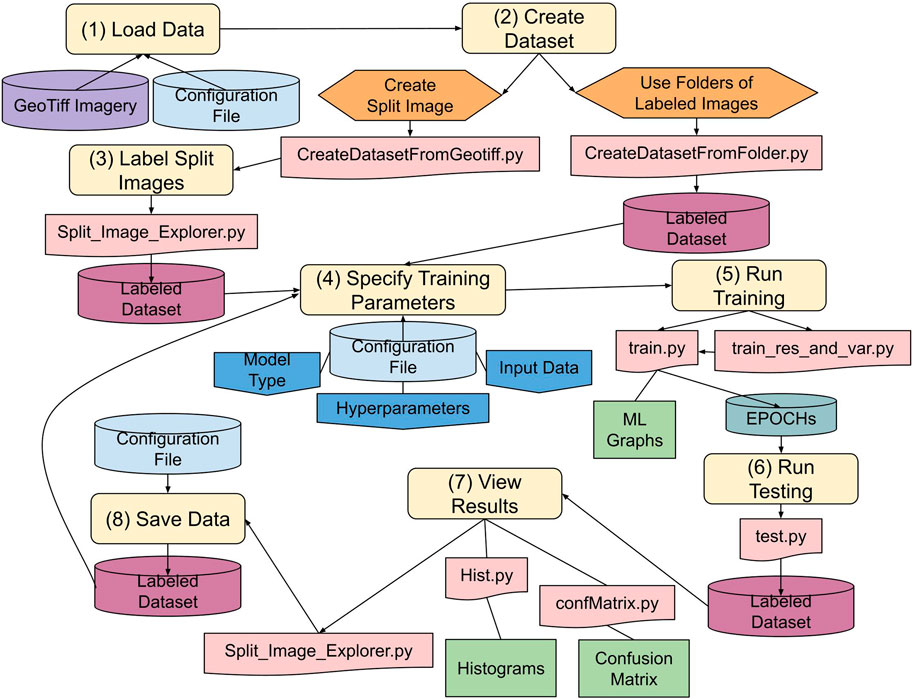
Figure 3. Flow diagram of GEOCLASS-image (v2.0), showing operation steps, inputs/outputs, datasets, configuration files and the feedback loop for dataset labeling and NN training.

The GEOCLASS-image workflow includes the following steps:

(1) Data Loading

(2) Dataset Creation

(3) Labeling of split-images

(4) Specification of Training Parameters

(5) Run Training

(6) Run Testing

(7) Visualization of Results

(8) Data Saving

2.1.1 High-level overview of the workflow

Data Loading (Step 1) includes visualization of one or several satellite images of the study area and provides utility tools that allow interaction of the user with the study area, here, the region of the Negribreen Glacier System, though a graphical user interface (GUI). Coordinate transformations are handled in this step. Central to the GEOCLASS approach is the identification of crevasse types, or other glacier surface types such as melt streams and melt ponds, in small subsets of the satellite image, called “split-images”. The creation of a good set of labeled training data is key to a successful classification and typically a bottleneck in the acceptance of a new ML approach in a geoscience discipline, as highlighted in the introduction. To this end, sets of split-images are created from a loaded satellite image in step (2) “Create Dataset” and then labeled in step (3) using the module “Split Image Explorer”. Alternative to using the GUI for data-set creation and labeling, crevasse classes can be identified for pre-existing split-images, stored in a directory with a subdirectory for each surface type class. A labeled dataset resultant from steps (2) and (3) is then ready for use in the training of several ML models in the next steps (4)–(7), with saving of the labeled data sets carried out in step (8). Repeating steps can be employed for optimizing the labeled training dataset, improving class association, and optimizing training parameters until a well-functioning NN model is achieved.

Step (4) summarizes specification of the NN architecture and related training parameters. GEOCLASS-image (v2.0) offers three machine learning models: These include a data-driven (ResNet-18), a physically driven (VarioMLP), and a combined (VarioNet) neural network type: The purely data-driven model looks at the unprocessed image values, whereas the physically driven model takes physically determined parameters derived from image values as input, and the combined model builds on both architectures. The integration of the two basic models, ResNet-18 and VarioMLP, into a computationally combined model constitutes one of the core advancements of GEOCLASS-image (v2.0) over GEOCLASS-image (v1.0), see Section 2.2. The diversity of ML models enables multiple approaches, enhancing the versatility of the cyberinfrastructure.

Steps (5)–(8) revolve around the creation and management of datasets. In order to satisfy the need of datasets in the cyrosciences, intuitive forms of dataset management and creation are necessary. This requires the user to be able to create and save large datasets in a condensed form to reduce the size of these files. These datasets must also be adjustable and easy to edit to increase usability. Once a dataset is created, the user must be able to use this to train and test at least one of the ML models. Through a feedback loop, steps (4)–(8) allow for variability in the parameters used to train each model which gives the user more control over the training and validation process. Once a model is trained, this model can then be used to classify all split-images in a dataset. One can then save these predictions to create large datasets (8), or use the predictions to train more complex models.

2.2 Advancement of surface classification in GEOCLASS-image (v2.0)

In this paper, we describe advancements of surface classification using the GEOCLASS-image CI on three different levels:

2.2.1 Utility functions

First, we introduce improvements to the technical implementation that are on the level of the user interface and the input/output of GEOCLASS. The most significant changes include the ability to write out training data sets. However, these changes facilitate the higher-level advancements of our NN infrastructure, the creation of shareable, labeled training data sets as are essential for advancing the use and broader acceptance of GEOCLASS by the glaciological and other science communities, where users may not have in-depth skills in ML. This addresses topic (2) discussed in the introduction.

2.2.2 Combined neural network architecture

A core piece of the work presented in this paper is the introduction of a new approach for the derivation of a combined neural network architecture (VarioNet) that leverages the advantages of two types of NNs, a physically driven neural network with a MLP for class association (VarioMLP) and a convolutional neural network (ResNet-18). The physically driven NN utilizes the connectionist-geostatistical classification method (Herzfeld and Zahner, 2001), which in itself combines two steps into a NN structure: The first step is an automated analysis of spatial structures detectable in high-resolution image data using vario functions, the second is a class association using a MLP. Central to the derivation of the combined NN architecture for VarioNet is a weighted fusion approach that includes one or several additional blocks in the sense of (He et al., 2016a), see Figure 4, as described in Section 4.3.

Figure 4

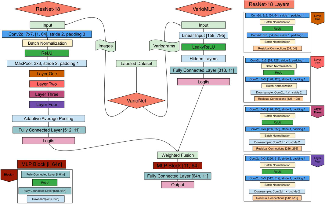
Figure 4. VarioNet NN design, architecture and training flow, integrating and combining ResNet-18 and VarioMLP by addition of a third NN architecture component. This third NN component consists of n MLP Blocks, specified by the user (here, n = 1) with the final dimension of the block equaling 64 $\cdot$ n. The input dimension, i, for these blocks is determined by n, with i corresponding to the total number of classes specified by the user for the first block, and i equaling 64 $\cdot$ n for all other blocks. The size of the final fully connected layer of each network also corresponds to the total number of classes specified by the user (here, 11).

The previous version GEOCLASS-image (v1.0) (Herzfeld et al., 2024) has facilitated an integration of the two approaches, “deep learning” and physically constrained neural networks. Representing the deep learning approach by the relatively shallow CNN, ResNet-18, and using the connectionist-geostatistical classification method implemented in the form of VarioMLP, we took the following approach for a synthesis of the two methods, creating VarioCNN: In essence, VarioMLP is employed to create optimized labeled data sets using a feed-back loop, which then were used to train VarioCNN, using the CNN, ResNet-18 for training. In contrast, VarioNet, to be developed in this paper, realizes a combination at the level of weighted fusion as a component of the neural network architecture.

2.2.3 Determination of weights in the fusion component of VarioNet

The two models, VarioMLP and ResNet-18, are being integrated using a weighting scheme, which is part of the combined structure for VarioNet. While it is easy to recognize that each model has its own advantages, the determination of weights that measure their respective contribution is a problem that we examine using two different approaches. First, we use a discrete optimization. Second, we explore and apply the concept of adaptive weighting.

2.2.4 Capturing the complexity of the surge process by a classification with 11 different crevasse and water-based ice-surface types

To capture the complex nature of a surge in an Arctic glacier system and the large variety of spatially heterogeneous surface structures that result from this process, we develop a classification scheme based on 11 distinct surface classes, which we use to create a labeled training dataset and subsequently to train the ML model, VarioNet. This capability is a step forwards towards the solution of the glaciological problem (Topic 1 in the introduction).

2.2.5 Upward compatibility

While the functionality of GEOCLASS-image (v2.0) is upward compatible with GEOCLASS-image (v1.0), the main benefits of the GEOCLASS-image (v2.0) CI result from its modular design. This allows for improvements and expansions as needed. Because the approach used for this software is modular, it can prove effective in a wide range of applications. Specifically, ML tactics and techniques can be easily applied to cryospheric problems allowing scientists to utilize the vast data currently accessible through Open Science practices. The GEOCLASS-image software also allows users to create their own labeled datasets without hand-labeling all the images. This feature is crucial to the cryospheric sciences and applications community, as large labeled training datasets are lacking, requiring scientists to hand-label datasets. While hand-labeled datasets may be more accurate, depending on the labeler, many ML models require large datasets on the magnitude of 10,000 images for generalized predictions (Krizhevsky et al., 2012; Herzfeld et al., 2024).

2.3 Geophysical application and data sets

The evolution of the current surge in the Negribreen Glacier System will be employed to evaluate the performance of the GEOCLASS-image software. To the end, we will utilize a crevasse-centered approach (Mayer and Herzfeld, 2000; Herzfeld et al., 2004; Trantow and Herzfeld, 2018; Herzfeld et al., 2022), building on the physical knowledge that crevasses are the surface signature of the deformation that results from glacial acceleration during the surge (Section 1 and see Mayer and Herzfeld (2000), Herzfeld et al. (2014), Herzfeld et al. (2024).

In order to study this glaciological phenomenon using GEOCLASS-image, high-resolution satellite imagery of the NGS from the surge is needed as input data. Specifically, sub-meter spatial resolution is required for the crevasse-centered approach. This requirement is met by the panchromatic band from Maxar’s WorldView satellites. The panchromatic band offers the highest resolution in WorldView and many other satellites, making it the most suitable source for spatial classification. Maxar satellites have collected optical satellite image data, which are available for cryospheric science uses as value-added products through the Polar Geospatial Center and the NASA Commercial SmallSat Data Acquisition (CSDA) Program, these are a widely used form of commercial imagery data (NASA, 2025; Polar Geospatial Center, 2025). Images for the tests of the GEOCLASS-image software range from May of 2016 to August of 2022 (Herzfeld et al., 2024). Each WorldView satellite has a revisit time of approximately 1.5 days, making it well-suited for monitoring the rapidly changing glaciological features of a surging glacier (Earth Observation Portal, 2023a; Earth Observation Portal, 2023b). However, WorldView data are optical image data and as such are affected by cloud cover, which often limits ground views in the Arctic. In consequence, only a relatively small number of useful datasets exist for the study of the surge in the NGS (Herzfeld et al., 2024). Airborne geophysical data, including image, time-lapse and lidar altimeter data, collected over the NGS in 2017, 2018, and 2019 by the second author and her group at the Geomathematics, Remote Sensing and Cryospheric Sciences Laboratory, University of Colorado Boulder, are used for evaluation of the labeled training data set and the results of the classification based on different neural network models derived here (Herzfeld and Trantow, 2021). This is used to determine the accuracy and effectiveness of the GEOCLASS-image software and the different machine learning models provided in its cyberinfrastructure.

The use of machine learning to classify complex crevasse structures has been demonstrated for other surge type glaciers such as the Bering-Bagley Glacier System, Alaska (Herzfeld and Zahner, 2001; Herzfeld et al., 2013), using nine classes. In the study that introduces and applies GEOCLASS-image (v1.0), six different crevasse classes are employed: Undisturbed Snow, One Directional, Multidirectional, Shear, Shear/Chaos, and Other. Here, we expand the surface types for the classification, as seen in Figure 5 to include water-based features: Melt Streams/Ponds and Sea Ice, along with nine crevasse-derived classes that are essential for capturing the complexity of the integrated ML system, VarioNet, developed in this work.

Figure 5

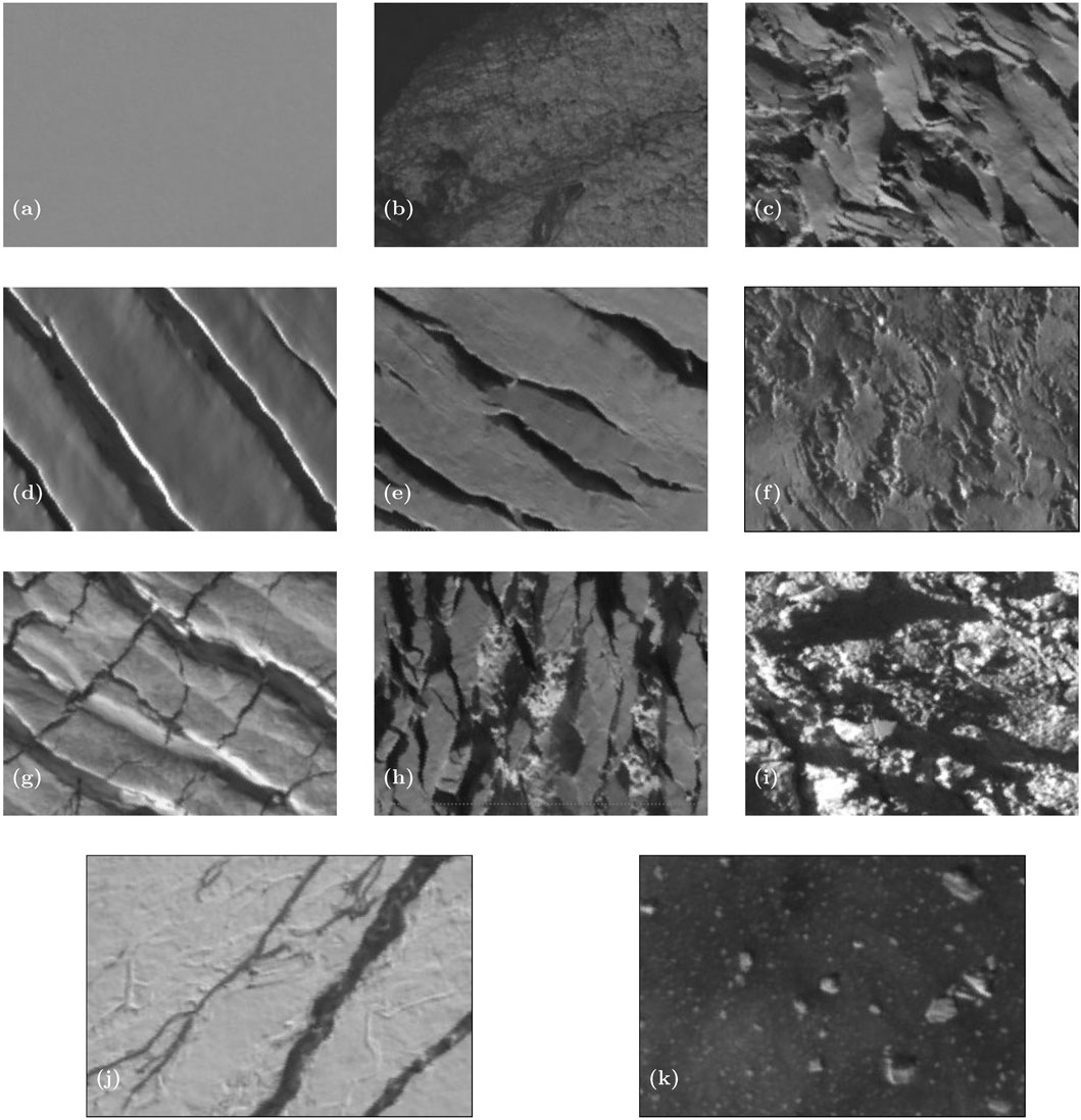
Figure 5. Example split-image for the physically derived crevasse classes. These classes were created based on the underlying physics and dynamics that cause the crevasse to form. (a) Class 1: Undisturbed Snow, (b) Class 2: Slow Moving Ice, (c) Class 3: Shear, (d) Class 4: Parallel, (e) Class 5: Parallel with Shear, (f) Class 6: Subordinate Shear, (g) Class 7: Multidirectional, (h) Class 8: Multigenerational, and (i) Class 9: Chaos. This figure also includes examples of split-images used for the water based classes (j) Class 10: Melt Streams and Melt Ponds, and (k) Class 11: Sea Ice. WorldView2 data set: WV02_20160625170309_1030010059AA
3500_16JUN25170309-P1BS-50080768
1050_01_P004_u16ns3413.tif. WorldView1 data set: WV01_20170530144716_1020010060152
E00_17MAY30144716-P1BS-5014817910
90_01_P004_u16ns3413.tif. WorldView1 data set: WV01_20180526211954_102001007158C
A00_18MAY26211954-P1BS-5023473130
40_01_P005_u16ns3413.tif.

3 Uprades to GEOCLASS-image utility functions

After the first release of the GEOCLASS-image CI many changes were made to the individual programs inside the CI. A number of small changes were implemented for optimization and to increase the ease of use of these programs; however, significant changes were made to increase the versatility of GEOCLASS-image. These upgrades were implemented to give the user more options for training, testing, creating datasets, and more. The goal of these improvements is to broaden the applications of the software and increase the user variability to fit individual needs. These modifications were also made for Open Science as it improved the output datasets available through this public software. In summary, software upgrades were installed to increase the versatility of input used, approaches used, and the output created.

3.1 Versatility of input

To derive a training data set, split-images are created from the WorldView data set and labeled by surface type (class type). In GEOCLASS-image (v1.0), the only way to view these labeled images, create datasets, and train the model was by use of the GUI. Due to the format of these datasets, one could only create a dataset for the specific area of interest, limiting the datasets to a single glacial system. The upgrades in GEOCLASS-image (v2.0) enable users to employ training images without geo-referencing data, from multiple glaciers and separate regions, which allows for more general datasets and classifications. In addition to using the GUI, labeled training images can now be exported into a directory that contains a subdirectory for each crevasse/surface class, thus facilitating application of the labeled training data sets within as well as independently of GEOCLASS-image. The new process allows us to create benchmark data sets in glaciology, suitable for assessment of classification approaches.

Another implementation for versatility of input comes in the sizing of the split-images created. While v1.0 already allowed the user to change the image size for a dataset, there was no reason for these images not to be square in shape as ResNet-18 excels with square images. For the second release of GEOCLASS-image it was deemed that the use of 3-4-5 images (sides proportional to 3 and 4, with the diagonal proportional to 5) could improve computation time and increase accuracy for VarioMLP. This geometry allows for pixel intensity values for real pixels as every lag step would relate to a pixel. Using square images with VarioMLP allowed for this along the sides of the image but the diagonal never corresponded to a real pixel value.

3.2 Versatility of output

In order to properly accommodate for the need of datasets in the cryospheric community, several enhancements to the CI were made allowing for greater versatility in the saving of datasets. Through a new variable in the configuration file, the user can now save all predictions in a dataset. Another addition to the configuration file allows the user to save “equal” datasets. This feature allows the user to create a dataset in which the class with the least associated images sets the maximum class size. For the other classes, the images with the highest confidence will be saved until the total number of images for that class is equal to the maximum class size. The confidence is calculated based on the probability that the image labeled by the model is the correct class, as formulated in Section 5.3.2. This minimizes the bias in the network and serves to prevent over-classification for classes with the largest number of images labeled.

4 Deriving a combined neural network

There are three approaches available to the user in GEOCLASS-image (v2.0): a data-driven approach through ResNet-18, a physically driven approach through the use of VarioMLP, and combination of the previous approaches with VarioNet. The data-driven approach has proven critical for many aspects of image recognition and classification. The reliance on every pixel causes this approach to have a high computational cost but will have a high accuracy if each class is visually different. The constraints of this approach can be seen in the networks inability to be validated with physical phenomena. With no physical constraints, the network can make predictions off incorrect patterns it finds leading to a poor performance on validation datasets.

Unlike the data-driven ResNet-18, VarioMLP is considered a physically driven approach due to the input data trained on. The network is driven based on vario functions, which give insight to the structural patterns found inside the image. These patterns occur on the basis of ice dynamics, which are confined by the physics of the glacier. Since vario functions are used to differentiate between the different physically derived patterns, it would reason that vario functions are physics-based data, making VarioMLP a physically driven approach (Herzfeld and Zahner, 2001). However, with increasing complexity, this approach decreases in effectiveness as different classifications of crevasses can cause similar underlying patterns that VarioMLP could mistake. The relationships between vario functions and surface signatures of the surge process are further described in Herzfeld et al. (2004), Herzfeld et al. (2024).

A new ML model, VarioNet, combines both approaches through a weighted fusion of the respective models’ outputs before passing this through a NN structure. The user can control the weight of each approach through the basic weight function $y=\alpha x+\beta x^{\prime }$ where $y$ is the input to the model, $\alpha$ and $\beta$ are the weights where $\alpha +\beta =1$, and $x$ and $x^{\prime }$ are the output of ResNet-18 and VarioMLP respectively.

4.1 VarioMLP

Given that crevasses form as a result of physical processes, a physically driven model can be expected to prove effective in their classification. VarioMLP is a physically driven multi-layer perceptron with back-propagation of errors that uses the geospatial data from the first order vario function of the image (Herzfeld and Zahner, 2001; Herzfeld et al., 2024). An example of how these vario functions may look can be seen in Figure 6. The vario function $\gamma$ is calculated based on Equation 1 for every valid pixel indexed by i, with the user specifying the total number of lag steps n.

$\gamma \left(h\right)=\frac{1}{2n}{\displaystyle \sum _{i=1}^n}{\left(z\left(x_i\right)-z\left(x_i+h\right)\right)}^2(1)$

Figure 6

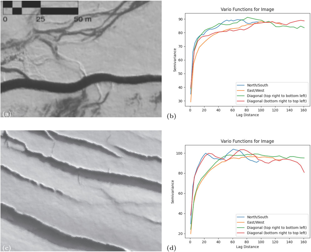
Figure 6. Visual and structural analysis for an example of two ice-surface classes, a melt stream (Class 10) and a parallel crevasse (Class 4). Structural analysis was conducted through the calculation of directional vario functions in GEOCLASS-image (v2.0). split-images selected from a WorldView-2 image from 06/26/2016 Note the visually similar appearance of the associated vario fucntions for both classes. Vario functions calculated with a lag step of three for the vertical, four for the horizontal, and five for the diagonal with a total of 33 lag steps. (a) Melt stream. (b) Directional vario function for melt stream split-image. (c) Parallel crevasse. (d) Directional vario function for parallel crevasse split-image. WorldView2 data set: WV02_20160625170309_1030010059AA
3500_16JUN25170309-P1BS-50080768
1050_01_P004_u16ns3413.tif.

In this equation $z(x_i)$ represents the pixel intensity taken at $x_i$, and h is the distance separating each measurement where $n\cdot x$ is the dimension of the image in that direction. To limit edge effects, a lag threshold is used to limit the range of the first pixel in each pair. The lag threshold will then determine the total lag-steps as the original dimension gets scaled by the lag threshold, and this becomes the maximum extent for the first point thus limiting the number of pairs. After the vario function is calculated in every direction, the image goes through a random rotation. This rotation is to account for the spatial variability across a crevasse, for instance, ice that only crevasses in a single direction would have differing vario functions depending on the direction of motion of the glacier, which varies spatially. From tests of how vario functions are effected by rotations and flips, it was determined that there are only four unique combinations of directional vario functions. Because of this, only three directional vario functions, horizontal, vertical, and one of the diagonals, are used as the input of VarioMLP. The architecture of VarioMLP revolves around an input node per vario-function value. For example, for an image with 33 lag-steps this would be 99 as there are three directions, each with 33 lag-steps. The size of the output node corresponds to the total number of classes being used as specified in the configuration program (Herzfeld and Zahner, 2001). The last variable for the architecture of VarioMLP is the number of hidden layers. The optimal hidden layer size found for the majority of ice-surface classification was [5,2]. Increasing the number of hidden layers can lead to an over-complication of the network typically resulting in overfitting (Herzfeld et al., 2024).

With the use of VarioMLP, the GEOCLASS-image approach does not require any preprocessing or data enhancement such as despeckling. The vario function component of the original connectionist-geostatistical method facilitates the extraction of spatial signatures from noisy data and data with missing pixels (Herzfeld and Zahner, 2001).

There are two different vario function scripts used for GEOCLASS-image. The first is only used when the split-images are of a certain size. If the split-images were saved in a shape proportional to a 3-4-5 rectangle, then this spatial characteristic is used to optimize the calculated vario function. This script uses the proportionality of the image to have a different lag step in each direction corresponding. For example, if an image of size [201, 268] was used with a lag-threshold of 0.5, the total lag number would be 33 as $\frac{201\cdot 0.5}{3}=\frac{268\cdot 0.5}{4}=33.5$ which is rounded down to 33. In the vertical direction the pixel intensity would be calculated every 3 pixels, in the horizontal every 4, and in the diagonal direction every 5 pixels. The advantages of using images of this proportion are two-fold as all the gray values are calculated from real pixels and the geometry allows for faster calculations. If an image does not have this intrinsic geometry, the image is cropped to its smallest dimension, then the lag step is calculated from the specified total amount of lag steps and the new dimensionality of the image. While calculating the vario functions for these images, the pixel intensity will be recalculated from the nearest pixel. This is due to the geometry of squares as the diagonal has the length of the sides multiplied by $\sqrt{2}$.

4.2 ResNet-18

Deep learning has led to many breakthroughs in image classification (He et al., 2016a; He et al., 2016b, He et al., 2021). ResNet-18 is a branch of widely used deep residual networks (ResNets) that has 18 deep layers, making it faster but less accurate than deeper versions of ResNet (He et al., 2016a). While there are many pretrained versions of ResNet-18 available for use, due to the lack of cryospheric datasets, the ResNet-18 architecture was used in the form available on pytorch. The main issue with using deep networks for image recognition is the degradation problem where network accuracy can decrease if the model passes a certain depth (He et al., 2016a). Another issue that is rather unique to the world of geosciences is the absence of physical validation of image classification. For deep, data-driven networks, like ResNet-18, image classification is based off raw pixel data. While this can be effective for many image classification problems, the network can form incorrect perceptions as there is no physical information being taken from the image. This limitation can be seen in the melt type classifications, image data may be similar to a crevasse but structurally they are very different. A second example of the limitations of ResNet-18 is the fact that it typically misclassifies Shear crevasses as will be demonstrated and analyzed in Section 6.2. In Figure 7a, ResNet-18 accurately predicts the images it is trained on but fails to perform as well on the validation dataset, resulting in overfitting. This flaw for geophysical application calls for the need of a combined approach that utilizes a data and physically driven machine leaning models (Reichstein et al., 2019).

Figure 7

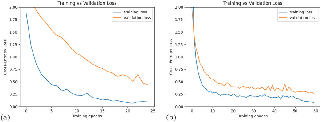
Figure 7. Graphs of training loss and validation loss, created during model training, used for model evaluation. (a) Example of an overfitting situation, from a ResNet-18 training run. While the training loss approaches zero, the validation loss remains high. Training and validation loss do not converge. (b) Example of a good training process, indicating good model performance. Validation and training losses decrease at similar rates and converge. Example from from the training of VarioNet with 50 normal epochs and 10 fine epochs.

4.3 VarioNet

The combination of data-driven and physically driven ML models is achieved with the creation of VarioNet, new in v2.0 of GEOCLASS-image. This ML model uses a data-fusion technique to combine the full architecture of VarioMLP and ResNet-18 as shown in Figure 4. The combined architecture allows for the network to make predictions based off structural patterns from the ice surfaces as well as utilizing deep residual learning based on the raw pixel data. A combined network can be more effective for structurally based image classification. VarioNet combines the important geospatial features unique to these complex classifications with modern ML to provide data and physically based predictions on structurally complex ice-surfaces.

In the flow diagram in Figure 4 we see that VarioNet is trained as follows: We train VarioMLP and ResNet 18 separately, using the same labeled training data set. Then, the raw outputs (in the form of logits, which are un-normalized scores the network assigns for each class per image) for each network are combined in a weighted fusion approach, illustrated by the curved flow arrows in Figure 4. The logits from both neural nets (VarioMLP and ResNet-18) become the inputs of a MLP. This MLP was coded to follow the logic and architecture of ResNet as described in He et al. (2016a) with a user-scalable depth to accommodate for a variety of classification tasks. The MLP consists of n blocks, where each block has (1) a fully connected layer that scales the input to a dimension of 64 $\cdot$ n, (2) ReLu activation, (3) another fully connected layer with same number of input nodes as output nodes, (4) a downsample layer with the same input and output dimensions as the first fully connected layer. Once the training data passes through all the blocks, the data is passed through a final fully connected layer with an output dimension equal to the total number of classes specified by the user.

While designing VarioNet, experiments were conducted to determine the optimal architecture. These trails included modifying the number of blocks, the scale factor, and the addition of a bottleneck layer as described by He et al. (2016a). VarioNet was tested with one, three, and five blocks, scale factors of 32, 64, 128, and 256, and bottleneck layers of various sizes were implemented at different points in the flow diagram. It was determined that for the classifications in this paper, VarioNet performed best with one block, no bottlenecks, and a scale factor of 64.

5 Application: surface classification, NN derivation, and optimization

5.1 Creation of dataset

To evaluate the performance of the three networks on geophysically confined classes, a relatively complex dataset was used for training. This dataset consists of nine classes which relate to the type of crevasse formed and two classes representing melt features (streams/ponds) and sea ice. The individual classes for this new dataset are as follows: Undisturbed Snow, Slow Moving Ice, Shear, Parallel, Parallel with Shear, Subordinate Shear, Multigenerational, Multidirectional, Chaos, Melt Streams/Ponds, and Sea Ice. These classes were developed by expanding upon previous classifications performed using the GEOCLASS-image CI (Herzfeld et al., 2024). Example split-images for each class can be visualized in Figure 5. A total of 750 split-images were labeled, with 600 images used for training and the other 150 images used for validation. With the exception of Melt Streams/Ponds and Sea Ice having 50 and 25 labeled images, respectively, 75 images were labeled for all crevasse-based classes to reduce biasing from an unequal dataset. As seen in Figure 8, these split-images were sourced from the following WorldView dataset: WV02_20160625170309, WV01_20170530144716, WV01_20180526211954. Given the high spatial, visual, and structural variability for Subordinate Shear, Melt Streams, Melt Ponds, and Sea Ice images, it was theorized that these would be the hardest classes to detect, and thus VarioNet should have the highest accuracy for these classes. ResNet-18 was hypothesized to excel for Undisturbed Snow, Slow Moving Ice and visually distinct crevasse classes such as Shear, Parallel, and Parallel with Shear. For more structurally complex classes such as Multigenerational, Multidirectional, and Chaos it was expected that VarioMLP would outperform ResNet-18.

Figure 8

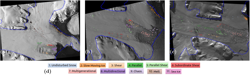
Figure 8. Labeled Dataset used for classification experiments. (a) Labeled images taken from the 2016 WV image, (b) images labeled from the 2017 WV dataset, (c) training and validation imagery from the 2018 WV image, and (d) legend for the labels WorldView2 data set: WV02_20160625170309_1030010059AA
3500_16JUN25170309-P1BS-50080768
1050_01_P004_u16ns3413.tif. WorldView1 data set: WV01_20170530144716_102001006015
2E00_17MAY30144716-P1BS-50148179
1090_01_P004_u16ns3413.tif. WorldView1 data set: WV01_20180526211954_102001007158
CA00_18MAY26211954-P1BS-50234731
3040_01_P005_u16ns3413.tif.

5.2 Training

Universal training and testing scripts are used in the GEOCLASS-image CI, allowing the user to specify all parameters in the configuration file and run one program for training and another for testing regardless of the model. In the configuration file, there are a variety of parameters the user can control to change how the models are trained. Some of these parameters are universal, such as the train with images parameter, while some are specific to the model being trained. The universal parameters are (1) train test split, (2) train with images, (3) use Compute Unified Device Architecture (CUDA), (4) number of epochs, (5) learning rate, (6) batch size, (7) activation and (8) optimizer which are standard parameters for NN training (Maas et al., 2013; Nair and Hinton, 2010; Kingma and Ba, 2014; Goodfellow et al., 2016; Luebke, 2008; Shorten and Khoshgoftaar, 2019) or specific to VarioMLP and introduced in (Herzfeld et al., 2024).

For the purposes of this paper, a train test split of 0.8 was used, meaning 80% of the labeled data was used for training while the other 20% was used for validation of the network. The network’s performance on the training and validation datasets is tracked using training and validation losses. These losses are calculated based on Equations 2 and 3 where L is the loss, N is the size of the dataset, C represents the total number of classes, $y$ represents the label for each split-image fed through a model and $\widehat{y}$ is the label predicted by the model.

$L=\frac{1}{N}{\displaystyle \sum _{i=1}^N}\text{Loss}\left(y_i,{\widehat{y}}_i\right)(2)$

$\text{Loss}\left(y,\widehat{y}\right)=-\frac{1}{N}{\displaystyle \sum _{i=1}^N}{\displaystyle \sum _{k=1}^C}{y}_{i,k}\log \left({\widehat{y}}_{i,k}\right)(3)$

These calculated losses are then saved in the form of a machine learning graph as seen in Figure 7. The graphs are used to determine network performance such as underfitting or overfitting. When a network performs well, both training and validation loss will be low and converge as the number of epochs increases, as exemplified in Figure 7b. Train with images, as the name entails, uses the folder of images specified in the configuration file to train the specified model if the variable is true. The use of CUDA allows for parallel computing using the computer’s graphics processing unit (GPU) to reduce training time. The rest of the universal parameters are parameters seen across machine learning applications and will vary based on the needs of the user. For the purposes of the experiments in this paper, a learning rate of 5e-5, batch size of 2, Leaky Rectified Linear Unit (Leaky ReLU) activation, and the Adam optimizer were used (Maas et al., 2013; Nair and Hinton, 2010; Kingma and Ba, 2014). For the number of epochs, multiple values were used. In order to observe the longterm behavior of each model, an epoch size of fifty was used. A high number of epochs was used to get a sense of over or under training as well as giving a good estimation of how many epochs were needed for an accurate prediction. The remaining training parameters are specific to VarioMLP or VarioNet (Herzfeld et al., 2024). As previously stated, VarioMLP allows for the user to specify the hidden layers. The user is also able to change the number of lag steps for the calculation of the vario function in the configuration file.

5.2.1 Training VarioNet

The input for VarioNet is a weighted combination of outputs produced by ResNet-18 and VarioMLP meaning the training processes is more involved than that of ResNet-18 or VarioMLP. Although VarioNet uses the same universal training and testing scripts used for ResNet-18 and VarioMLP, to get optimal weights for ResNet-18 and VarioMLP, the user has to run a separate training program. This program trains ResNet-18 and VarioMLP on the labeled dataset and their weights are saved inside the working folder. This feature allows VarioNet to load pre-trained versions of these networks in order to increase the accuracy of the combined network. Once the weights of ResNet-18 and VarioMLP are saved, one can run the universal training and testing scripts on VarioNet. It’s important to note that after training ResNet-18 and VarioMLP, a variable called train indices will be updated in the configuration file. This is to ensure that the same images are being used for training and validation while training Resnet-18 and VarioMLP as when training VarioNet to minimize bias. While training VarioNet, there are two stages to optimize the training process. First, VarioNet is trained the same way the other models are trained, using the same number of epochs and learning rate to get a general classification. Next, the training program ensures that all of the weights are unfrozen and the learning rate is lowered to fine tune the whole network. The latter stage will train the network for the amount of time specified by the number of fine epochs in the configuration file.

5.3 Experiments for optimization of weights in a fused neural network

To investigate the relative importance of integrating two different NN types, a CNN and a physically driven MLP, into a single neural network structure, we conducted three experiments to optimize the weights of the respective NN types. The first approach is discrete optimization to determine optimal weights. The second and third approaches utilize adaptive weighting, with different formulas for weight determination.

5.3.1 Discrete weight optimization

To find the optimal weights for VarioNet with fusion, the lowest validation loss achieved during training and the validation accuracy of the network were tracked. The optimal weights were determined using a stepwise discrete optimization with an interval of 0.1. As seen in Table 1, the resultant optimally weighted combined NN is achieved by weights of $\beta =0.45$ for ResNet18 and $\alpha =0.55$ for VarioMLP. Surprisingly, VarioNet performed adequately regardless of the weights as the accuracy on the validation dataset never dropped below 91%. This indicates that VarioNet extracts necessary information from the input logits, despite how the logits were weighted before fusion. For example, when driven with $\alpha =0.95$ and $\beta =0.05$ VarioNet had an accuracy of 92.5%, even though VarioMLP had an accuracy of 52.3%, see Section 6.1. This is significant because it suggests that the superior performance is intrinsic to the architecture of VarioNet.

Table 1

Table 1. 11 Class fusion weights sensitivity study.

5.3.2 Adaptive weight optimization

To avoid the need of sensitivity studies for future classification tasks, an option was added to automatically calculate fusion weights for each image, motivated by an approach described in Zhang et al. (2018) where the confidence of a CNN is used to determine whether a model should use a CNN or MLP to classify each image.

The confidence for each network is calculated from each logit, defined in Equation 4 where z is the logit, W is the weights matrix, x is the input feature vector, and b is the bias vector. The confidence, derived from the softmax function described in Equation 5, gives an array of length N where $z_n\in [\mathrm{0,1}]$ and ${\sum }_1^N{z}_n=1$, where n is the indexed class and N is the total number of classes. For each class n, the output from the softmax function of $z_n$ represent the probabilities that the image belongs to class n. The predicted class for each image is then selected based on the class with the highest confidence.

The idea of adaptive weighting is that the weights are initialized using a softmax function, which can either depend on the confidence of the CNN alone (Equation 6) or be formulated in a symmetric fashion using the confidence of both network types (Equation 7). The adaptive weighting process evaluates confidence for each small batch of training images and then recalculates the measure as the process continues. This is illustrated in Figure 9.

Figure 9

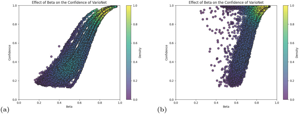
Figure 9. Plots showing the effect of beta, the weight of ResNet-18, on the confidence of VarioNet on testing data. Points are colored by density with the scale showing the normalized densities that range from zero to one. (a) This plot shows which beta values were used for training data when beta was calculated based off the confidence of ResNet-18. (b) This plot was created from the same dataset as (a) but beta was calculated based on both ResNet-18’s and VarioMLP’s confidence.

Following a similar logic as that used by Zhang et al. (2018), the first method of adaptive fusion was derived. For this method, the weight of ResNet-18, $\beta$, is determined from the confidence of ResNet-18 as seen in Equation 6. For the second method, it was assumed that when ResNet-18’s confidence is low, VarioMLP’s confidence would also be low, and that the most accurate prediction would come from VarioNet using approximately equally weighted logits from both VarioMLP and ResNet-18. The equation for $\beta$ for this method can be found in Equation 7 with z representing the logits from ResNet-18 and y representing the logits from VarioMLP. For every method the weight of VarioMLP was determined by the following equation: $\alpha =1-\beta$ where $\alpha ,\beta \in [\mathrm{0,1}]$.

The distributions of $\beta$, as seen in Figure 9, shows the confidence of VarioNet increasing as $\beta$ increases for both methods. Incorporating the inverse confidence of VarioMLP increases the overall accuracy of VarioNet, the accuracy of VarioNet at lower values of $\beta$, and the average value of $\beta$. From these findings it was determined that the second method is more robust and accurate and was therefore implemented in VarioNet for the second release of GEOCLASS-image.

$\mathbf{z}=Wx+b(4)$

$\text{softmax}\left(z_n\right)=\frac{e^{z_n}}{{\sum }_{j=1}^N{e}^{z_j}},\text{for\hspace{0.17em}}n=\mathrm{1,2},\dots ,N(5)$

$\beta =Max\left(softmax\left(z\right)\right)(6)$

$\beta =\frac{Max\left(softmax\left(z\right)\right)+\left[1-Max\left(softmax\left(y\right)\right)\right]}{2}(7)$

As seen in Figure 9a, adaptive weighting with Equation 6 tends to result in a close correlation between $\beta$ and the confidence of VarioNet. This nearly linear relation indicates that the adaptive weighting process is not able to shift effectively between the weights of MLP and CNN. Therefore, the logic behind using a combined model is rendered useless as its performance is exclusively dependent on one of the approaches. Equation 7 resulted in a more even weighting with lower $\beta$ values relating to high confidence for VarioNet as seen in Figure 9. As a result of the symmetrical approach taken with Equation 7, VarioNet is able to shift away from the CNN and towards a balanced weighting between ResNet-18 and VarioMLP for the optimally combined result.

5.3.3 Optimized weighted fusion

For a visual comparison in the difference of discrete and adaptive fusion using Equation 7, both trained models of VarioNet were used to classify all split-images over the NGS from the WV dataset described in Section 5.1. The resulting predictions can be seen in Figure 10, where both models resulted in a very similar spatial distribution of classes. These similarities can also be visualized in Figure 11a with discrete weighting resulting in a slightly higher accuracy for Class 6: Subordinate Shear. Adaptive weighting resulted in an accuracy of 92.5% without fine tuning and as seen in Table 2, an accuracy of 95.5% with the optimal fine tuning learning rates. Discrete weighting was able to slightly increase the accuracy of VarioNet on the validation dataset to 94.0%. However, as can be visualized in Figure 11b, fine tuning decreased the accuracy of VarioNet on Subordinate Shear meaning the total accuracy the fine-tuned discretely weighted model of VarioNet barely increased to 94.1%.

Figure 10

Figure 10. Classification results from VarioNet trained with discrete (a–c) and adaptive (d–f) weighting. For adaptive weighting, Equation 7 was used to determine fusion weights. Classifications are arranged in chronological order from 2016 (a, d) till 2018 (c, f). The two weighting methods result in nearly identical predictions for the 11 classes (g). WorldView2 data set: WV02_20160625170309_1030010059AA
3500_16JUN25170309-P1BS-50080768
1050_01_P004_u16ns3413.tif. WorldView1 data set: WV01_20170530144716_102001006015
2E00_17MAY30144716-P1BS-50148179
1090_01_P004_u16ns3413.tif. WorldView1 data set : WV01_20180526211954_102001007158
CA00_18MAY26211954-P1BS-50234731
3040_01_P005_u16ns3413.tif.

Figure 11

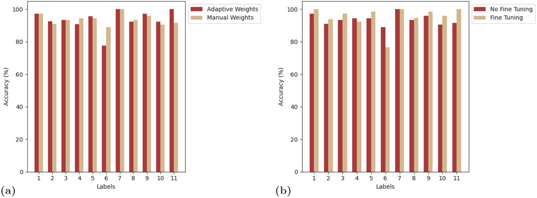
Figure 11. Histograms to visualize how VarioNet behaves under different training conditions. VarioNet was trained and validated with the same dataset where the accuracy for each class was calculated based on the validation dataset. (a) This graph shows the effect of adaptive weighting on the accuracy of VarioNet for a 11 class prediction. The light tan histograms shows the optimal weights found from Table 1 where the weight of ResNet-18 was 0.45 and 0.55 was the weight for VarioMLP. The dark brown histograms represent the accuracy of VarioNet when using adaptive weights. Both tests were trained without fine tuning. (b) This histogram shows the effect of fine tuning VarioNet. The light tan bars represent an additional 10 fine epochs with a learning rate of 5e-6, where the dark brown relates to training without fine tuning. The same discrete weights as in (a) were used for both tests. The labels correspond to the classes as seen in Figure 14J.

Table 2

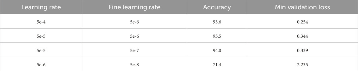
Table 2. Learning rate sensitivity study, training and testing were conducted with the same dataset over 50 normal and 10 fine epochs, using adaptive weighting.

Overall, discrete weighting will give less freedom to the network, decreasing training time and allow the user to gain a better sense of how the weights of ResNet-18 and VarioMLP will affect the predictions from VarioNet based on the classification task. Adaptive weighting will increase training time as it recalculates the fusion weights for ResNet-18 and VarioMLP each batch. As a result, this method can be used for more complex classification tasks where the optimal fusion weights vary heavily depending on the class. As shown in Table 1, VarioNet performed consistently across different weightings, indicating that recalculating weights by batch will have minimal impact on classification results for this study.

6 Application and validation

After VarioNet, ResNet-18 and VarioMLP were trained with the same hyperparameters, as detailed in Section 5.2, the epoch with the lowest validation loss was selected from the plots in Figure 12 for each model. Using the GEOCLASS-image CI, the models were loaded with weights corresponding to the epoch selected for each model: 49 for VarioNet, 48 for ResNet-18 and 42 for VarioMLP. These trained models were then applied to classify all 33,234 split-images from the same WorldView dataset used for labeling, as described in Section 5.1. The GUI allows individual analysis of each model’s prediction and confidence levels, as well as comparison of the full-scale spatial class distribution against prior domain knowledge for validation. The CI also allows for a quantitative analysis through the validation dataset created during training.

Figure 12

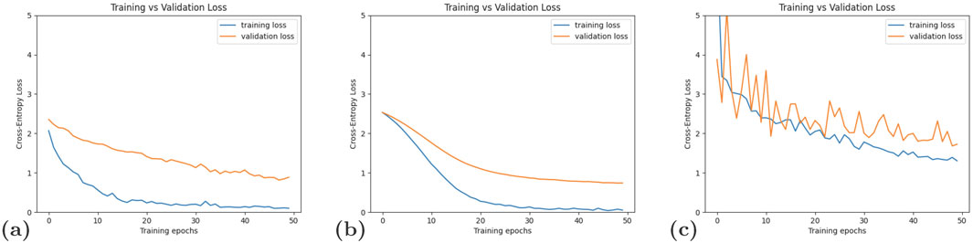
Figure 12. Training and validation loss graphs for the 11 class predictions from the three NN types trained. All networks were trained and validated with the same dataset and hyperparameters for 50 epochs. (a) Smooth training loss graph for ResNet-18 showing overfitting. (b) Smooth raining loss graph for VarioNet showing slight overfitting. (c) Noisy training loss graph for VarioMLP showing overfitting.

6.1 Validation dataset analysis

The complete labeled dataset created by each model, VarioNet, ResNet-18 and VarioMLP, was subset to only include the split-images that were used for validation through the variable train indices as described in Section 5.2. These datasets were then used to determine each network’s overall accuracy as well as give a class-by-class analysis as seen in Figures 11, 13. As detailed in Section 5.3.3, VarioNet performed adequately regardless of the fusion method used. As seen in Figure 11a, discrete weighting resulted in better accuracy for Subordinate Shear, but a lower accuracy for Sea Ice when compared to discrete weighting. With 10 epochs of fine tuning, the accuracy from discrete weighting for Subordinate Shear drastically decreased, as seen in Figure 11b. This resulted in the overall accuracy on the validation dataset increasing from 94.0% to 94.1%. With adaptive weights, the accuracy of VarioNet slightly decreased to 92.5% when trained for 50 epochs, but increased up to 95.5% from fine tuning with the optimal learning rate as seen in Table 2.

Figure 13

Figure 13. Histogram for the accuracy of the three NN types, ResNet-18 (dark brown), VarioNet (tan), and VarioMLP (purple), trained on the same 11 class dataset. VarioNet was trained using the optimal discrete weights found in Table 1, all networks were trained with the same hyperparameters for the same number of epochs, 50. The labels correspond to the classes as seen in Figure 14j.

The accuracy of the three models is evaluated for each ice-surface class in Figure 13. Of the three models, VarioNet resulted in the highest validation accuracy for Slow Moving Ice, Parallel, Subordinate Shear and Multigenerational Crevasses. On the other hand, VarioNet did not have the lowest accuracy for any class, compared to ResNet-18 and VarioMLP. As a result, this combined NN resulted in the highest accuracy when compared to the other networks available through GEOCLASS-image. Although ResNet-18 labeled more of the validation dataset correctly for the following classes: Unidsturbed Snow, Shear, Parallel with Shear, Melt Streams/Ponds and Sea Ice, it had an overall accuracy of 89.2%. This decrease in overall accuracy is the result of relatively poor performance for Subordinate Shear and Multidirectional crevasses. While VarioMLP labeled only 52.3% of validation images correctly, this model correctly labeled 100% of the validation images for the Multidirectional and Chaos classes. VarioMLP performed the worst on Shear crevasses in the validation dataset, having a lower than 40% accuracy for Shear and Subordinate Shear. However, as seen in Section 6.2 VarioMLP has a tendency to correctly classify the shear types, while also producing false positives.

6.2 Geophysical validation and interpretation

The time series of the three classifications from VarioMLP, ResNet-18 and VarioNet allow a geophysical interpretation of the evolution of the surge in the NGS, based on surface signatures of two types of geophysical processes that occur during the surge: (1) Deformation and (2) occurrence of supraglacial water (see, Figure 14). The interpretation is based on the results from this classification, augmented by airborne field observations of the surge and satellite image analysis (Herzfeld et al., 2024; Herzfeld et al., 2021; Herzfeld et al., 2022; Trantow and Herzfeld, 2024b). In 2016, the surge had affected only a small area near the calving front of the glacier. The surge started upstream of the calving front, in a region where three heavily crevassed across-flow regions are seen in Figure 8a and then quickly progressed downglacier, reaching the calving front by the time the 2016 imagery was collected. All three models capture the complex crevasse types (Shear, Subordinate Shear, Multidirectional) in the 2016 image correctly, however, there are significant differences in the correct association of the individual classes by each network. Generally, VarioMLP and VarioNet individually perform well at detecting the longitudinally oriented regimes, whereas ResNet-18 is best at recognizing the transverse-oriented crevasse fields as Multidirectional.

Figure 14

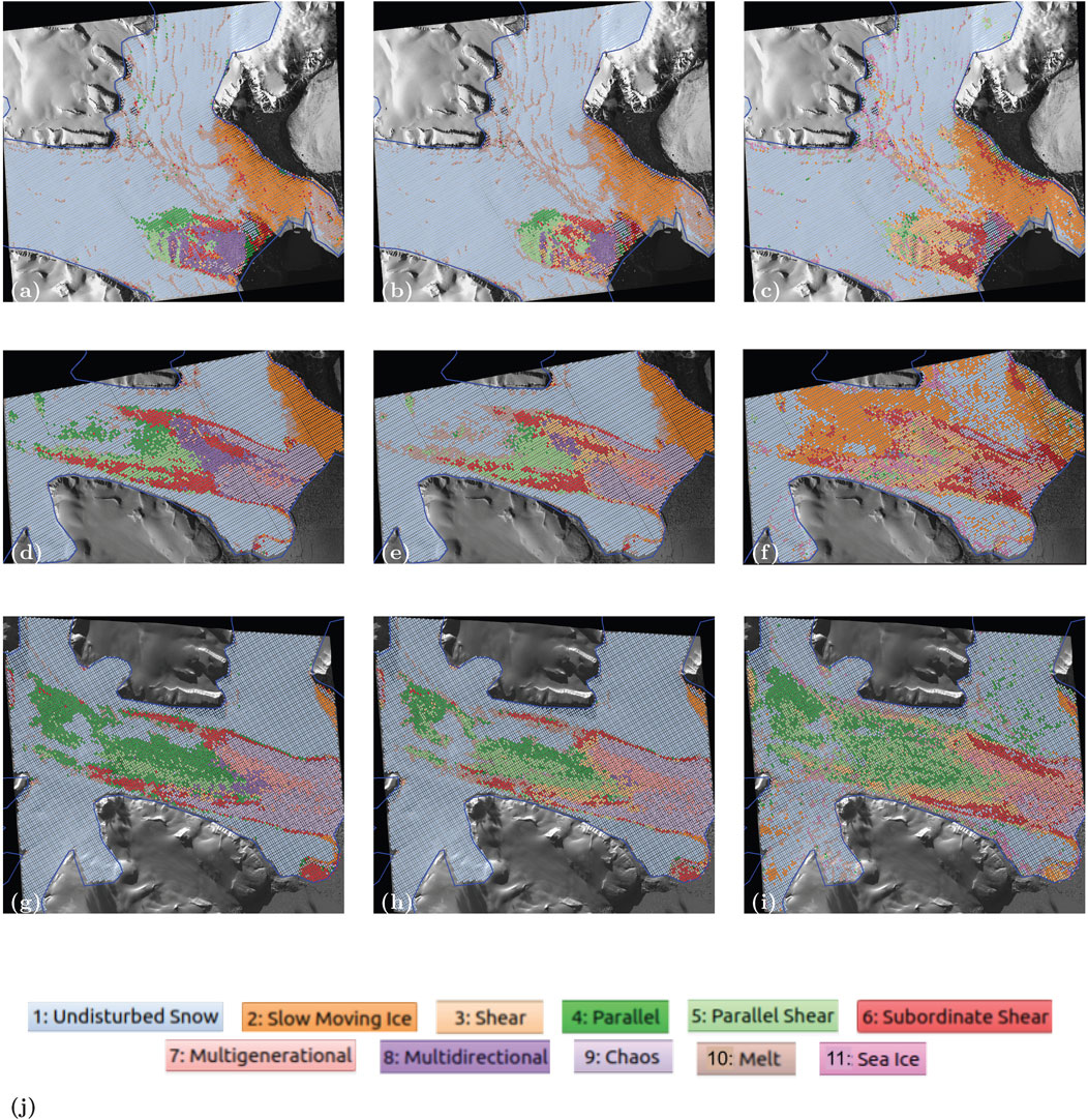
Figure 14. Results of ice-surface classifications from three NN types for the evolution of NGS from June 2016 to May 2018 visualized through WorldView-1 and WorldView-2 imagery. All the networks were trained and validated with the same dataset. VarioNet was trained using the optimal discrete weights found in Table 1. (a) Classification resultant from ResNet-18 for 2016. (b) Classification resultant from VarioNet for 2016. (c) Classification resultant from VarioMLP for 2016. (d) Classification resultant from ResNet-18 for 2017. (e) Classification resultant from VarioNet for 2017. (f) Classification resultant from VarioMLP for 2017. (g) Classification resultant from ResNet-18 for 2018. (h) Classification resultant from VarioNet for 2018. (i) Classification resultant from VarioMLP for 2018. (j) Legend for the classifications results. WorldView2 data set: WV02_20160625170309_1030010059AA
3500_16JUN25170309-P1BS-50080768
1050_01_P004_u16ns3413.tif. WorldView1 data set: WV01_20170530144716_102001006015
2E00_17MAY30144716-P1BS-50148179
1090_01_P004_u16ns3413.tif. WorldView1 data set: WV01_20180526211954_102001007158
CA00_18MAY26211954-P1BS-50234731
3040_01_P005_u16ns3413.tif.

New to this classification is the inclusion of water-based surface classes, specifically, Melt Streams/Ponds and Sea Ice. The Sea Ice class was introduced to prevent misclassification in the region in front of the calving front, where, during the surge, large amounts of calved ice mixed with seasonally receding sea ice (see, Figures 2a,b). Inclusion of the Sea Ice type is largely needed because the location of the ice front changed rapidly during the surge. Trantow and Herzfeld (2024b) observed the formation of a retreating bay in July 2017, an area between Ordonnansbreen and Negribreen, which was partly filled with icebergs and partly with open water. A similar scenario may explain the identification of a smooth surface (labeled as Undisturbed Snow by VarioMLP, Figure 14c).

The occurrence of surface melt streams is typical for slow-moving ice, which characterizes the entire Ordonnansbreen (the side glacier joining Negribreen from the north, Figure 1; cf. Figure 2f). VarioNet classifies Melt Streams/Ponds correctly, an ability that is inherited from ResNet-18.

An essential component of the classification of structural surface signatures, or results of deformation in general, is the ability to classify Shear (Herzfeld et al., 2004). Shear is almost completely missed by ResNet-18, which is a result of the solely data-driven classification of ResNets and CNNs in general (Herzfeld et al., 2024). VarioMLP tends to correctly identify shear types, however, it also renders false positives. VarioNet has an ability to overcome both these deficiencies. This ability is a key property of the VarioNet approach.

Parallel and Parallel Shear always occur in the uppermost regions of the area that has been affected by the surge expansion. This characteristic is captured to some extent by all three neural network types across all three years. As the kinematic wave of the surge advances into non-surging ice, thin parallel crevasses form first (see, (Herzfeld et al., 2021), and the imagery included there). Parallel Shear should occur between regions of Parallel and Shear, something ResNet-18 fails to demonstrate. VarioNet tends to label one-directional crevasses as Parallel Shear as opposed to just Parallel. VarioMLP has a tendency to correctly classify Parallel Shear, more so than the class Parallel. For these classes as well, VarioNet results in the best recognition and classification of Parallel and Parallel Shear.

Some misclassifications that occur may be attributed to differences in surface reflectance in the original imagery, as opposed to differences in structural change. For example, the class Slow Moving Ice in the 2016 and 2017 classification maps does include Slow Moving Ice, however, the extent of Slow Moving Ice is much larger than the orange regions. Differences in material properties such as progressing firn saturation affect the classification likely as a result of a labeling bias.

A definite strength of the neural network experiments presented here is that the thematic maps resultant from VarioNet correctly show the expansion of the surge and the location of the shear zones, which are features that have escaped many previous mapping attempts. Especially, the shear along the northern and southern margins, depicted as Subordinate Shear. ResNet-18 applied to the 2017 imagery (Figure 14d) has a tendency to misclassify Multidirectional, where the actual classes are Multigenerational or Shear. VarioNet does better in this regard. In general, the complex classes of Chaos and Multigenerational/Multidirectional are difficult to differentiate. The summer of 2017 marked the height of the acceleration in Negribreen, rendering complex deformation that transformed pre-existing crevasse types to Multigenerational and Chaos. In VarioNet, these classes indeed dominate in the lower region of the NGS, encompassing the area where crevassing already occurred in 2016, and adjacent areas. Among the three models, VarioNet excels at identifying regions where the ice was still undisturbed, labeled here in a simplified fashion as Undisturbed Snow.

In summary, VarioMLP demonstrates strong performance in capturing structurally complex patterns, while ResNet-18 is more effective at recognizing spatially simpler imagery in areas that deviate significantly from the training data. Closer analysis shows that only a few split-images were selected from the 2016 transverse crevasse fields for training. Overall, VarioMLP demonstrates a distinct ability to distinguish between classes that appear similar in pattern but differ in crevasse formation, which is driven by ice surface deformation during spatially complex transformations. VarioNet has the ability to overcome the weaknesses of the input models, ResNet-18 and VarioMLP, and as a result, the time series of maps resultant from VarioNet renders the best representation of the crevasse provinces and their evolution during the surge in 2016–2018. In addition, VarioNet produces the highest confidence for evolution of the surge. As seen in Figure 15, ResNet-18 has a high confidence for uncrevassed regions, but this confidence drastically drops in the heavily crevassed central regions. Although VarioMLP has low confidence for all regions of the NGS, VarioNet is able to classify the crevassed areas with a higher confidence than ResNet-18.

Figure 15

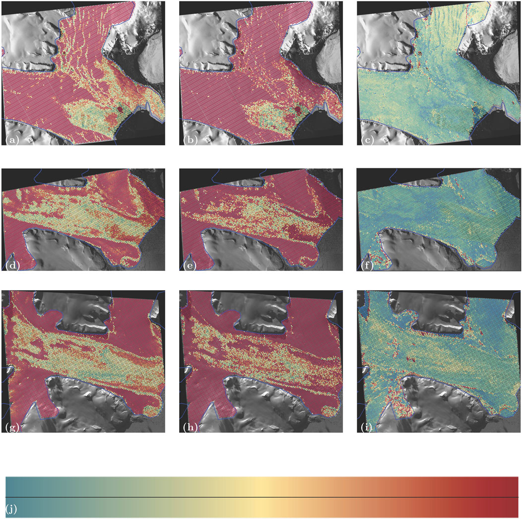
Figure 15. Results of ice-surface classifications from three NN types for the evolution of NGS from June 2016 to May 2018 visualized through WorldView-1 and WorldView-2 imagery. All the networks were trained and validated with the same dataset. VarioNet was trained using the optimal discrete weights found in Table 1 (a) Confidence resultant from ResNet-18 for 2016. (b) Confidence resultant from VarioNet for 2016. (c) Confidence resultant from VarioMLP for 2016. (d) Confidence resultant from ResNet-18 for 2017. (e) Confidence resultant from VarioNet for 2017. (f) Confidence resultant from VarioMLP for 2017. (g) Confidence resultant from ResNet-18 for 2018. (h) Confidence resultant from VarioNet for 2018. (i) Confidence resultant from VarioMLP for 2018. (j) Legend for confidence results. WorldView2 data set: WV02_20160625170309_1030010059AA
3500_16JUN25170309-P1BS-50080768
1050_01_P004_u16ns3413.tif. WorldView1 data set: WV01_20170530144716_102001006015
2E00_17MAY30144716-P1BS-50148179
1090_01_P004_u16ns3413.tif. WorldView1 data set: WV01_20180526211954_102001007158
CA00_18MAY26211954-P1BS-50234731
3040_01_P005_u16ns3413.tif.

The approach taken in this paper, as visualized in Figure 4, to combine a data-driven CNN and a physically based MLP, successfully created a network that overcomes the shortcomings of each individual approach. VarioNet combines the advantages of both models, ResNet-18 and VarioMLP, rendering a NN model that allows classification of a structurally large and complex region (33,234 split-images) from a labeled data set of 750 images with a 80/20% split for training and validation data.

7 Summary, conclusions and outlook

7.1 Summary

GEOCLASS-image is a CI for classification of ice-surface types of glaciers based on high-resolution satellite image data. The software has been implemented for application to MAXAR WorldView1 and WorldView 2 imagery.

The objective of this paper is to describe and demonstrate the capabilities of the second release of GEOCLASS-image. Specifically, to showcase a new NN that combines a data and physically based approach. This paper also serves as a software description with a more detailed walkthrough of the software that is available on GitHub (Herzfeld et al., 2025).

The new version includes several generalizations and capabilities that increase the applicability and versatility of the software significantly. The main achievements that set GEOCLASS-image (v2.0) apart from GEOCLASS-image (v1.0) (Herzfeld et al., 2023) are as follows:

(1) Labeled training data sets: Version 2.0 presents a solution to the problem of creating labeled training data for cryospheric problems for which such data do not currently exist.

(2) GEOCLASS-image (v2.0) includes an approach for the derivation and training of a new NN architecture, termed VarioNet, that combines the advantages of a data-driven and physically driven NNs, by integrating the physically driven VarioMLP with the data-driven ResNet-18 through introduction of an additional NN component.

As seen in Table 3, the main functionalities of GEOCLASS-image can be broken down into subsections with the majority of implemented improvements for GEOCLASS-image (v2.0) relating to the management of datasets. Most of these improvements appeal to the ease of use and versatility and aim to broaden the applications of the software.

Table 3

Table 3. Main features of GEOCLASS-image in release v1.0 and v2.0.

7.2 Main results

7.2.1 Versatility of input and output

GEOCLASS-image (v1.0) was created with a user-friendly GUI to offer an appealing framework for users in the cryospheric science and applications community that would not require much understanding of ML. However, the GUI-centered approach resulted in some limitations, which have been resolved in v2.0 through implementation of several improvements regarding versatility of data input and output. GEOCLASS-image (v2.0) now offers options for user-friendly, system immanent training and application using the GUI, as well as for importing and exporting datasets to facilitate interoperability with other software, essential for advancing Open Science. For input, GEOCLASS-image has the ability to include additional images outside of the area of interest, which may complement images selected from the uploaded WorldView data, resulting, for example, from a different application. For output, in addition to using the GUI, labeled training images can now be exported into a directory that contains a subdirectory for each crevasse/surface class, thus facilitating application of the labeled training data sets within and independently of GEOCLASS-image. The new process allows us to create benchmark data sets in glaciology, suitable for assessment of classification approaches.

7.2.2 Open science

Open Science calls for sharing and improving the accessibility of datasets, which the updates to the GEOCLASS-image infrastructure hope to accomplish as they and have been tested to ensure ease of use and functionality. The biggest improvement for Open Science comes from the changes to the Split Image Explorer. The Split Image Explorer has been modified to specifically aid in the creation of datasets for the cryospheric community. These changes not only simplify the process of saving datasets, but also added needed options to customize these datasets. All of these options have been created with ease of use in mind and can be modified through the configuration file allowing users to easily switch between desired settings. In addition, these improvements allow users to create datasets with the same amount of images in each class, for the desired classes, a feature implemented to improve the effectiveness of labeled training datasets for machine learning applications. Lastly, another important upgrade is an option for saving predictions from multiple scenes. Now the user is able to save every single prediction above a specified confidence threshold, which allows for the creation of larger and more accurate datasets.

7.2.3 VarioNet

The publication of GEOCLASS-image (v2.0) includes a prototype combined neural network (VarioNet) that takes structural calculations, previously realized in the connectionist-geostatistical approach that results in VarioMLP, and input directly from images, as is typical in CNNs for image classification, specifically ResNet-18. VarioNet employs a data fusion approach as follows: VarioMLP and ResNet-18 are first trained separately, using the same labeled training dataset. In a second training step, the raw outputs of VarioMLP and ResNet-18, or so-called logits (unnormalized scores the network assigns for each class per image), are combined and passed through one or several additional NN blocks. These logits are then fused together through discrete or adaptive weighting. VarioNet includes a two-step training process where the latter stage lowers the learning rate and re-trains to fine-tune the model for the classification of more complex ice surfaces. The VarioNet approach facilitates differentiation between visually or structurally similar classes. This type of data fusion approach allows the user to leverage the effect each network has on the final network. The benefits of this approach are apparent when comparing the prediction maps created by each NN available through GEOCLASS-image. Specifically, VarioNet performs best in situations where classes originally missed by the data-based approach are over classified by the physically-based approach. This is best exemplified in the Shear and Sea Ice classes in Figure 14.

7.3 Conclusion

An efficient, scientific software tool should be easy to use, expandable, accurate, and tested rigorously. The GEOCLASS-image (v2.0) CI serves to aid remote sensing analysis conducted by cryospheric scientists and offers an intuitive, user friendly tool that facilitates image classification over complex ice surfaces. The GEOCLASS-image software is designed using a modular approach that allows for improvements and expansions. For the second release of GEOCLASS-image, the modularity of the design was tested through the addition of new features, programs, and a new model architecture. The additional features and NN were tested through ice-surface classifications for the current surge in the NGS. The multitude of different crevasse classes that occur in close proximity as a consequence of the rapid transformation of the glacier surface during surge makes the NGS an ideal testbed for the creation of a NN that combines the advantages of a physically constrained NN and a data-driven CNN. The resultant NN can be expected to generalize to other types of glacier systems, such as those in Greenland, Alaska and the Canadian Archipelago.

Through the classification of the NGS with each type of NN, it is evident that VarioNet is a promising combined approach for image classification of complex geophysical processes, such as the surge of an Arctic glacier. The predictions produced by VarioNet were nearly identical for discrete and adaptive weighting, hinting at the importance of the NN block utilized by VarioNet. With both weighting methods VarioNet is capable of overcoming the shortcomings of the data-driven ResNet-18 and physically based VarioMLP to produce a more geophysically accurate prediction for the surge of the NGS from 2016 until 2018.

The second release of GEOCLASS-image has only been tested with Linux Ubuntu 22.04.4 and used for the Negribreen Glacier System, Svalbard, and a basic classification of the Bering Glacier System, Alaska.

7.4 Outlook

The GEOCLASS-image cyberinfrastructure, realized here for Maxar WorldView1 and WorldView2 satellite imagery, can be expected to generalize easily to classification of any high-resolution satellite imagery. Applications in this study are carried our for a specific cryospheric sciences problem, the classification of glacier surface types, but computationally similar applications can be envisioned in other geoscience disciplines, including land surface classification, land-cover/land-use classification and sea-ice classification.

Data availability statement

The datasets presented in this study can be found in online repositories. The names of the repository/repositories and accession number(s) can be found below: https://github.com/Herzfeld-Lab/GEOCLASS-image/releases/tag/v2.0.

Author contributions

ST: Conceptualization, Formal Analysis, Investigation, Methodology, Software, Validation, Visualization, Writing – original draft, Writing – review and editing. UH: Conceptualization, Funding acquisition, Methodology, Project administration, Resources, Supervision, Writing – original draft, Writing – review and editing. TT: Conceptualization, Data curation, Methodology, Supervision, Visualization, Writing – original draft, Writing – review and editing.

Funding

The author(s) declare that financial support was received for the research and/or publication of this article. The work in this paper was primarily funded by U.S. National Science Foundation (NSF) Office of Advanced Cyberinfrastructure award OAC-1835256. Research on the surge in the NGS and data collection were supported by the U.S. National Aeronautics and Space Administration (NASA) Earth Sciences Division under awards 80NSSC20K0975, 80NSSC18K1439 and NNX17AG75G and by the U.S. National Science Foundation (NSF) under awards OPP-1745705 and OPP-1942356 (Office of Polar Programs). Research on WorldView data analysis was also supported by NASA Earth Sciences under the CSDAP. Principal Investigator for all awards is Ute Herzfeld. Helicopter support was facilitated by the Norwegian Polar Center. Collection of airborne data in Svalbard was conducted with permission of the National Security Authority of Norway, the Civil Aviation Authority of Norway and the Governor of Svalbard, registered as Research in Svalbard Project RIS-10827 “NEGRIBREEN SURGE”. The data collection was also partly supported through a 2018 Access Pilot Project (2017_0010) of the Svalbard Integrated Observing System (SIOS). All this support is gratefully acknowledged.

Acknowledgments

Thanks are due to Jack Hessburg, Tasha Markley, Adam Hayes, Rachel Middleton, Griffin Hale, Lukas Goetz-Weiss, Alex Weltman, Alfredo de La Pena Gonzales, Connor Meyers and Chris Higginson, all Geomathematics Lab, University of Colorado Boulder, to Oliver Zahner for previous work on the classification methods and the GEOCLASS software. Maxar WorldView satellite imagery from the surge of the Negribreen Glacier System was acquired with help from the Polar Geospatial Center, University of Minnesota, here we are indebted to Paul Morin, Jonathan Pundsack, Cole Kelleher, Stephanie Linde and colleagues, and through the NASA Commercial Small Satellite Program (CSDAP).

Conflict of interest

The authors declare that the research was conducted in the absence of any commercial or financial relationships that could be construed as a potential conflict of interest.

Generative AI statement

The author(s) declare that no Generative AI was used in the creation of this manuscript.

Publisher’s note

All claims expressed in this article are solely those of the authors and do not necessarily represent those of their affiliated organizations, or those of the publisher, the editors and the reviewers. Any product that may be evaluated in this article, or claim that may be made by its manufacturer, is not guaranteed or endorsed by the publisher.

Supplementary material

The Supplementary Material for this article can be found online at: https://www.frontiersin.org/articles/10.3389/feart.2025.1572982/full#supplementary-material

References

Camps-Valls, G., Tuia, D., Zhu, X. X., and Reichstein, M. (2021). Deep learning for the Earth Sciences: a comprehensive approach to remote sensing, climate science and geosciences. John Wiley and Sons.

Google Scholar

Deng, J., Dong, W., Socher, R., Li, L. J., Li, K., and Fei-Fei, L. (2009). “Imagenet: a large-scale hierarchical image database,” in 2009 IEEE conference on computer vision and pattern recognition (IEEE), 248–255.

Google Scholar

Earth Observation Portal (EOPortal) (2023a). Worldview-1. Available online at: https://www.eoportal.org/satellite-missions/worldview-1. (Accessed February 1, 2024).

Google Scholar

Earth Observation Portal (EOPortal) (2023b). Worldview-2. Available online at: https://www.eoportal.org/satellite-missions/worldview-2 (Accessed February 1, 2024).

Google Scholar

Goodfellow, I., Bengio, Y., and Courville, A. (2016). Deep learning. MIT press.

Google Scholar

Harrison, W., and Post, A. (2003). How much do we really know about glacier surging?. Ann. Glaciol. 36, 1–6. doi:10.3189/172756403781816185

CrossRef Full Text | Google Scholar

He, K., Zhang, X., Ren, S., and Sun, J. (2016a). “Deep residual learning for image recognition,” in Proceedings of the IEEE conference on computer vision and pattern recognition, 770–778.

Google Scholar

He, K., Zhang, X., Ren, S., and Sun, J. (2016b). “Identity mappings in deep residual networks,” in Computer vision–ECCV 2016: 14th European conference, Amsterdam, The Netherlands, october 11–14, 2016, proceedings, Part IV 14 (Springer), 630–645.

Google Scholar

He, Z., Li, J., Liu, L., He, D., and Xiao, M. (2021). Multiframe video satellite image super-resolution via attention-based residual learning. IEEE Trans. Geoscience Remote Sens. 60, 1–15. doi:10.1109/tgrs.2021.3072381

CrossRef Full Text | Google Scholar

Herzfeld, U., McDonald, B., and Weltman, A. (2013). Bering Glacier and Bagley Ice Valley surge 2011: crevasse classification as an approach to map deformation stages and surge progression. Ann. Glaciol. 54 (63), 279–286. doi:10.3189/2013aog63a338

CrossRef Full Text | Google Scholar

Herzfeld, U., Trantow, T., Lawson, M., Hans, J., and Medley, G. (2021). Surface heights and crevasse types of surging and fast-moving glaciers from ICESat-2 laser altimeter data — application of the density-dimension algorithm (DDA-ice) and validation using airborne altimeter and Planet SkySat data. Sci. Remote Sens. 3, 1–20. doi:10.1016/j.srs.2020.100013

CrossRef Full Text | Google Scholar

Herzfeld, U. C., Clarke, G. K. C., Mayer, H., and Greve, R. (2004). Derivation of deformation characteristics in fast-moving glaciers. Comput. and Geosciences 30, 291–302. doi:10.1016/j.cageo.2003.10.012

CrossRef Full Text | Google Scholar

Herzfeld, U. C., Hessburg, J., Hayes, A., and Trantow, T. (2023). GEOCLASS-image (v1.0). Available online at: https://github.com/Herzfeld-Lab/GEOCLASS-image/releases/tag/v1.0. (Accessed February 1, 2024). doi:10.5281/zenodo.10232912

CrossRef Full Text | Google Scholar

Herzfeld, U. C., Hessburg, L. J., Trantow, T. M., and Hayes, A. N. (2024). Combining “deep learning” and physically constrained neural networks to derive complex glaciological change processes from modern high-resolution satellite imagery: application of the GEOCLASS-image system to create VarioCNN for glacier surges. Remote Sens. 16, 1854. doi:10.3390/rs16111854

CrossRef Full Text | Google Scholar

Herzfeld, U. C., Lawson, M., Trantow, T., and Nylen, T. (2022). Airborne validation of ICESat-2 ATLAS data over crevassed surfaces and other complex glacial environments: results from experiments of laser altimeter and kinematic GPS data collection from a helicopter over a surging Arctic glacier (negribreen, svalbard). Remote Sens. 14, 1185–1224. doi:10.3390/rs14051185

CrossRef Full Text | Google Scholar

Herzfeld, U. C., McDonald, B., Wallin, B. F., Krabill, W., Manizade, S., Sonntag, J., et al. (2014). Elevation changes and dynamic provinces of Jakobshavn Isbræ, Greenland, derived using generalized spatial surface roughness from ICESat GLAS and ATM data. J. Glaciol. 60, 834–848. doi:10.3189/2014JoG13J129

CrossRef Full Text | Google Scholar

Herzfeld, U. C., and Trantow, T. (2021). Airborne laser altimeter, global positioning system (GPS), inertial measurement unit (IMU) and imagery campaign of the surging Negribreen Glacier, svalbard. Available online at: https://arcticdata.io/catalog/view/ (Accessed February 1, 2024).

Google Scholar

Herzfeld, U. C., Twickler, S., and Trantow, T. (2025). GEOCLASS-image (v2.0). Available online at: https://github.com/Herzfeld-Lab/GEOCLASS-image/releases/tag/v2.0 (Accessed February 1, 2024).

Google Scholar

Herzfeld, U. C., and Zahner, O. (2001). A connectionist-geostatistical approach to automated image classification, applied to the analysis of crevasse patterns in surging ice. Comput. and Geosciences 27, 499–512. doi:10.1016/S0098-3004(00)00089-3

CrossRef Full Text | Google Scholar

Huang, G., Liu, Z., Van Der Maaten, L., and Weinberger, K. Q. (2017). “Densely connected convolutional networks,” in Proceedings of the IEEE conference on computer vision and pattern recognition, 4700–4708.

Google Scholar

Jiskoot, H. (2011). Glacier surging. Encycl. Snow, Ice Glaciers, 415–428. doi:10.1007/978-90-481-2642-2_559

CrossRef Full Text | Google Scholar

Kingma, D. P., and Ba, J. (2014). Adam: a method for stochastic optimization. arXiv Prepr. arXiv:1412.6980. doi:10.48550/arXiv.1412.6980

CrossRef Full Text | Google Scholar

Krizhevsky, A., Sutskever, I., and Hinton, G. E. (2012). Imagenet classification with deep convolutional neural networks. Adv. neural Inf. Process. Syst. 25.

Google Scholar

Lefauconnier, B., and Hagen, J. O. (1991). Surging and calving glaciers in eastern Svalbard. Meddelelser, Nor. Polarinst. 116, 1–133.

Google Scholar

Lin, M., Chen, Q., and Yan, S. (2013). Network in network. arXiv Prepr. arXiv:1312.4400. doi:10.48550/arXiv.1312.4400

CrossRef Full Text | Google Scholar

Liu, X., Hu, Q., Cai, Y., and Cai, Z. (2020). Extreme learning machine-based ensemble transfer learning for hyperspectral image classification. IEEE J. Sel. Top. Appl. Earth Observations Remote Sens. 13, 3892–3902. doi:10.1109/jstars.2020.3006879

CrossRef Full Text | Google Scholar

Luebke, D. (2008). “Cuda: scalable parallel programming for high-performance scientific computing,” in 2008 5th IEEE international symposium on biomedical imaging: from nano to macro (IEEE), 836–838.

Google Scholar

Maas, A. L., Hannun, A. Y., and Ng, A. Y. (2013). “Rectifier nonlinearities improve neural network acoustic models,” in Proc. icml (Atlanta, GA), 3.

Google Scholar

Mayer, H., and Herzfeld, U. (2000). Structural glaciology of the fast-moving jakobshavn isbræ, Greenland, compared to the surging Bering Glacier, Alaska, USA. Ann. Glaciol. 30, 243–249. doi:10.3189/172756400781820543

CrossRef Full Text | Google Scholar

Meyer, H., and Pebesma, E. (2021). “Estimating the area of applicability of remote sensing-based machine learning models with limited training data,” in 2021 IEEE international geoscience and remote sensing symposium IGARSS (IEEE), 2028–2030.

Google Scholar

Nair, V., and Hinton, G. E. (2010). “Rectified linear units improve restricted Boltzmann machines,” in Proceedings of the 27th international conference on machine learning (Haifa, Israel: ICML-10), 807–814.

Google Scholar

NASA (2025). Smallsat data evaluation. Available online at: https://www.earthdata.nasa.gov/about/csda/smallsat-data-evaluation (Accessed February 1, 2024).

Google Scholar

Polar Geospatial Center (2025). Polar geospatial center, data + services. Available online at: https://www.pgc.umn.edu/data/ (Accessed February 1, 2024).

Google Scholar

Reichstein, M., Camps-Valls, G., Stevens, B., Jung, M., Denzler, J., Carvalhais, N., et al. (2019). Deep learning and process understanding for data-driven earth system science. Nature 566, 195–204. doi:10.1038/s41586-019-0912-1

PubMed Abstract | CrossRef Full Text | Google Scholar

Shorten, C., and Khoshgoftaar, T. M. (2019). A survey on image data augmentation for deep learning. J. big data 6, 60–48. doi:10.1186/s40537-019-0197-0

CrossRef Full Text | Google Scholar

Simonyan, K., and Zisserman, A. (2014). Very deep convolutional networks for large-scale image recognition. arXiv:1409.1556.

Google Scholar

Song, J., Gao, S., Zhu, Y., and Ma, C. (2019). A survey of remote sensing image classification based on CNNs. Big earth data 3, 232–254. doi:10.1080/20964471.2019.1657720

CrossRef Full Text | Google Scholar

Tai, C., Xiao, T., Zhang, Y., Wang, X., and Wainan, E., (2015). Convolutional neural networks with low-rank regularization. arXiv Prepr. arXiv:1511.06067. doi:10.48550/arXiv.1511.06067

CrossRef Full Text | Google Scholar

Trantow, T., and Herzfeld, U. C. (2018). Crevasses as indicators of surge dynamics in the Bering Bagley Glacier System, Alaska: numerical experiments and comparison to image data analysis. J. Geophys. Res. Earth Surf. 123, 1615–1637. doi:10.1029/2017JF004341

CrossRef Full Text | Google Scholar

Trantow, T., and Herzfeld, U. C. (2024a). Evolution of a surge cycle of the bering-bagley Glacier System from observations and numerical modeling. J. Geophys. Res. Earth Surf. 129, e2023JF007306. doi:10.1029/2023JF007306

CrossRef Full Text | Google Scholar

Trantow, T., and Herzfeld, U. C. (2024b). Progression of the surge in the Negribreen Glacier System from two years of ICESat-2 measurements. J. Glaciol. doi:10.31223/X5NT1Z

CrossRef Full Text | Google Scholar

Virts, K., Shirey, A., Priftis, G., Ankur, K., Ramasubramanian, M., Muhammad, H., et al. (2020). “A quantitative analysis on the use of supervised machine learning in earth science,” in IGARSS 2020-2020 IEEE international geoscience and remote sensing symposium (IEEE), 2252–2255.

Google Scholar

Xiang, C., Zhang, L., Tang, Y., Zou, W., and Xu, C. (2018). MS-CapsNet: a novel multi-scale capsule network. IEEE Signal Process. Lett. 25, 1850–1854. doi:10.1109/lsp.2018.2873892

CrossRef Full Text | Google Scholar

Zhang, C., Pan, X., Li, H., Gardiner, A., Sargent, I., Hare, J., et al. (2018). A hybrid MLP-CNN classifier for very fine resolution remotely sensed image classification. ISPRS J. Photogrammetry Remote Sens. 140, 133–144. doi:10.1016/j.isprsjprs.2017.07.014

CrossRef Full Text | Google Scholar