An exploration of the relative influence of physical models for Omori’s law

Omori’s law states that the rate of aftershocks decays as a function of inverse time. There are multiple physical explanations that we reduce into a nonlinear mixed effects relation of three terms: (1) a Rate/State expression that can account for static/dynamic and viscoelastic triggering caused directly by the mainshock, (2) a fluid diffusion triggering term, and (3) a randomized secondary triggering (cascade) term. We fit free physical-model parameters to an observed aftershock sequence through two nonlinear regression methods to find the relative contributions of physics-based models in an observed aftershock sequence. Results from both methods show that Rate/State models overpredict aftershock rates by ∼0–30%. Secondary aftershocks cause a net negative contribution (seismicity rate reduction that corrects overprediction by other terms) ranging between ∼0 and 30%. All regression solutions yield negative secondary triggering contributions without being guided to do so. A physical explanation for this is that aftershock occurrence relieves stress from the crust, ultimately causing the sequence to extinguish itself. Fluid diffusion triggering contributions range from ∼0 to 20%. Diffusion processes are observed to be shorter in time than the full duration of an aftershock sequence and they are also spatially limited, diminishing their influence. Our results apply to an aftershock decay curve from the 2016 Central Apennines earthquake sequence, meaning that our specific results may not be general. Our primary conclusion is that any one physical model cannot alone fit the observed sequence as well as the combination of three we investigated.

1 Introduction

Aftershocks are defined as events of generally lesser magnitude following a larger main shock that are distributed around the fracture area of the main shock (e.g., Uidas, 1999). In 1894, Fusakichi Omori observed that the rate of aftershocks decays as the inverse of time following a main shock (Omori and Coll, 1894). An improved fit to observed aftershock rates can be made by applying Tokuji Utsu’s (1961) formulation as k/(c + t)^p, where k, c, and p, are constants that can vary with different sequences, with the exponent p usually ranging from ∼0.7 to 1.5. Additional modifications to Utsu’s formula were made by Shcherbakov et al. (2004) to incorporate earthquake magnitude scaling laws, as did Hainzl and Marsan (2008). It was noted by Utsu et al. (1995) that the Epidemic Type Aftershock Sequence (ETAS) models by Yosihiko Ogata (e.g., Ogata, 1988) achieved an improved representation of aftershock characteristics because these models account for secondary triggering (cascades) of earthquakes by aftershocks of the main shock (e.g., Ogata, 1998; Ziv, 2003).

In this paper we explore fits of a blend of physics-based aftershock rate models to observations through regression methods. We assess the relative roles of acknowledged physical causes of earthquake triggering to better understand their role in Omori’s law under the possibility that more than one cause is operating in any given aftershock sequence. We consider three primary modes of earthquake triggering within aftershock sequences and their relationships to Omori’s law: (1) static stress and/or dynamic triggering caused by slip of the mainshock, (2) fluid diffusion triggering, and (3) secondary triggering through aftershock cascades by static and dynamic earthquake triggering. Each of these triggering modes have physics-based explanations for Omori’s law. We explicitly do not include models that identify parameters based on empirical observations, and the point of this study is to see if any one, or a blend of physical models can fit observations. We do not intend to solve aftershock occurrence globally. This paper is instead intended to show a method on how we might assess the relative roles of different physical models/concepts in aftershock sequences. We intentionally fit a single aftershock sequence that is associated with a very high-resolution catalog as a proof of concept.

We combine relations describing the three triggering modes into one equation and we minimize the number of free parameters by combining constants together to broadly represent the physics of aftershock triggering. We use that relation and its parameters to fit an observed aftershock sequence from a high-resolution earthquake catalog of the 2016 Central Apennines, Italy earthquake sequence that is complete to M1.04 (Tan et al., 2021). We focus on the 64-day series following the initial mainshock, the M6.0 Amatrice earthquake, because this well-studied, high-quality catalog occurred in a region where there is evidence that multiple physical processes influencing aftershock occurrences have occurred. We use two different nonlinear regression methods for fitting to assess method dependence.

2 Physical models for aftershock occurrence

Aftershocks occurring on or near the rupture plane have been explained as a result of incomplete mainshock rupture and/or heterogeneous slip (e.g., Bullen and Bolt, 1985). Elastic strain caused by the mainshock has also been invoked to explain aftershocks away from the primary rupture plane as early as Clarence Dutton’s (1904, p. 62) statement, ‘‘. . . portions of the raised or sunken mass are subject to stresses which from time to time give rise to further movements. . . .’‘. Dutton’s (1904) and Bullen and Bolt’s (1985) explanations are consistent with modern concepts of stress transfer caused by fault slip that mostly correlate with the spatial pattern of off-fault aftershocks (Figure 1) (e.g., Harris, 1998 and references therein; Stein, 1999; Freed, 2005). Mancini et al. (2019) showed that static stress-based forecasting during the 2016 Central Apennines sequence was as effective as statistical ETAS simulations, particularly when secondary triggering by M ≥ 3 earthquakes was included.

Figure 1

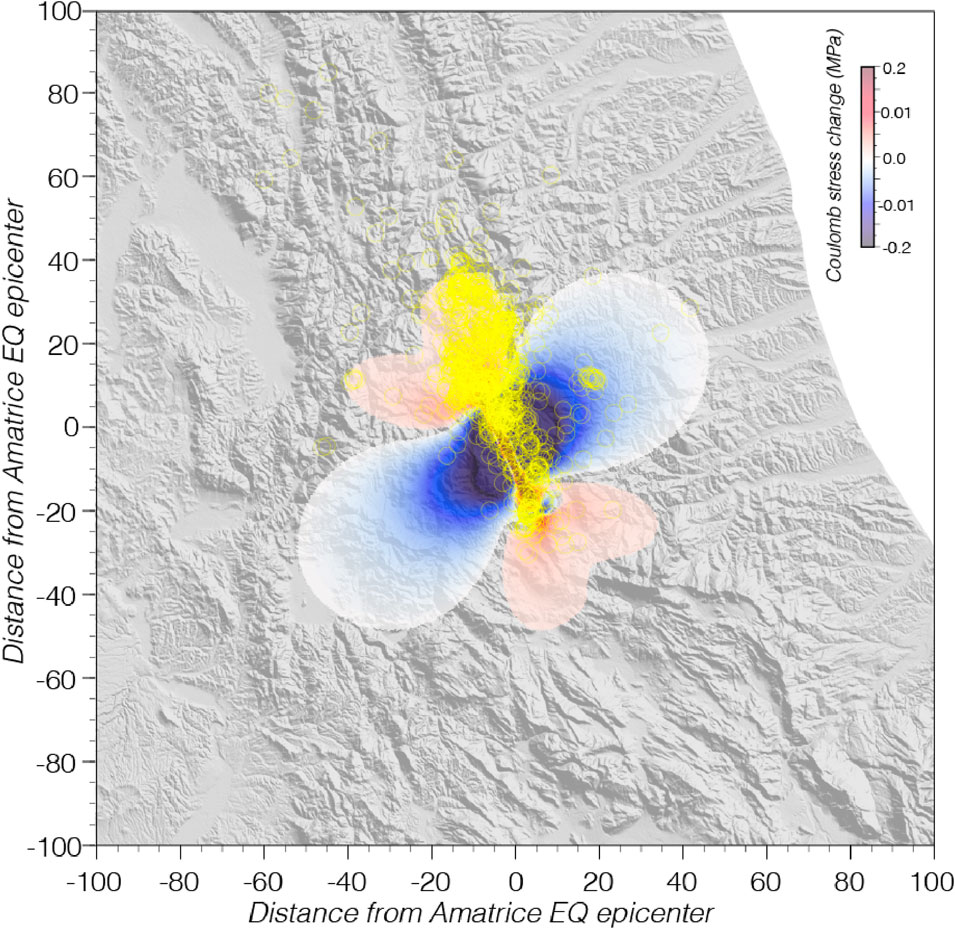
Figure 1. Example Coulomb spatial forecast of earthquake activity (M ≥ 3) following the 24 August 2016 M = 6.2 Amatrice mainshock in central Italy. Aftershock epicenters (yellow circles) are superposed on static stress change calculations made after the mainshock up until the Visso (October 26, 2016) Red colors show regions of increased failure stress (up to 0.2 MPa), and blue decreased (stress shadows). Note that not all aftershocks can be explained by the initial static stress change but may be caused by dynamic and/or secondary triggering.

It is also well established that earthquakes can be triggered by changes in pore fluid pressure that can alter the frictional state and contact area on a locked fault by forcing it open (Biot, 1941; Hubbert and Rubey, 1959). Human induced pore fluid pressure changes are observed to trigger earthquakes (Evans, 1966; Ellsworth, 2013 and references contained therein), and observations have also been made of fluid pressure changes caused by an earthquake that in turn triggers other earthquakes (e.g., Nur and Booker, 1972; Malagnini et al., 2012; Tung and Masterlark, 2018; Albano et al., 2019; Miller, 2020; Kato, 2024). Fluid diffusion triggering is observed within the Central Apennines mainshock sequence (e.g., Albano et al., 2019; Chiarabba, et al., 2020; Malagnini et al., 2022) (Figures 2, 3). In Figure 2, earthquake clusters are identified that have distinct progressions through time (t) and space (d) as $d\left(t\right)\propto \sqrt{t}$ in a similar mode as observed in the Apennines by Malagnini et al. (2012).

Figure 2

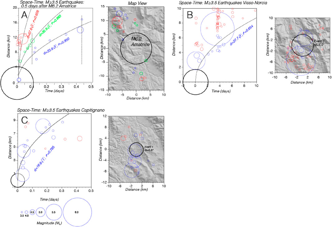
Figure 2. Diffusion vs. time as interpreted by fitting time sequences to functions of t-^1/2, and spatial migration from Malagnini et al. (2022). (A) three different simultaneous diffusion processes may be recognized, mostly to the north of the Amatrice main shock. Map view to the right. (B) Diffusion process associated with the mainshocks of Visso (October 26, 2016) and Norcia (October 30, 2016), with a map view to the right. (C) Capitignano. Diffusion process associated to the seismic sequence of Capitignano (January 18, 2017). Map view to the right.

Figure 3

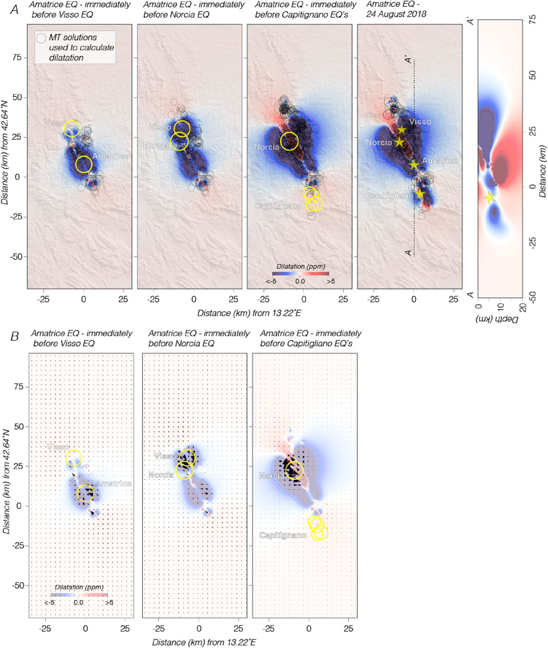
Figure 3. (A) Cumulative dilatation is calculated by Malagnini et al. (2022) assuming the SW dipping moment tensor solutions of M ≥ 3 earthquakes were the rupture planes. Yellow circles are events associated with potential diffusion triggering shown in Figure 2. Dilatation is shown on horizontal planes at 5 km depth, and a cross section is shown to the right. (B) Expected relative flow magnitudes and directions resulting from coseismic dilatation changes caused by M ≥ 3 earthquakes beginning with the 24 August 2016 Amatrice earthquake to times just before the Visso, Norcia, and Capitignano earthquakes.

Additionally, elastic dislocation modeling by Malagnini et al. (2022) of dilatation induced by mainshocks within the 2016 Central Apennines sequence and modeled fluid flow changes imply that higher fluid pressures might be expected at sequential mainshock locations (Figure 3). While not proving a pore fluid pressure earthquake triggering mode, these models and observations are consistent with the process. That and the abundant observations of human induced earthquakes (e.g., Evans, 1966; Ellsworth, 2013 and references contained therein) support the inclusion of a fluid diffusion model in our exploration.

Earthquakes are also observed to be triggered dynamically by passing seismic waves (e.g., Hill et al., 1993). The predominant indicator of dynamic triggering is that its aftershock spatial decay is more gradual than that from a static stress change, which diminishes as a function of distance d, as d^-3. Dynamic triggering close to the mainshock is most likely caused by shorter period direct P- and S-wave phases with amplitudes that decay with distance more gradually than static stresses (e.g., Parsons and Velasco, 2009). Interpretations of observed spatial aftershock decay rates vary (e.g., Felzer and Brodsky, 2006; Richards-Dinger et al., 2010), making it difficult to determine how important dynamic triggering is in the near source region. Earthquakes can be triggered at global distances by longer period surface waves (e.g., Velasco et al., 2008; Parsons et al., 2014 and references contained therein). The proportion of earthquakes triggered dynamically was estimated to be 34% vs. 66% static triggering after 3 M ≥ 7.0 California mainshocks by Hardebeck and Harris (2022), based on the occurrence of aftershocks in static stress-reduced areas (also visible in Figure 1). Similarly, Parsons (2002) found a ratio of 31% dynamic vs. 69% static triggering from M ≥ 5 aftershocks of global M ≥ 7.0 mainshocks.

Post mainshock viscoelastic relaxation in the deep crust and upper mantle can increase stresses on upper crustal faults that trigger earthquakes, and the duration of these processes can be much longer than the early phases of aftershock production (e.g., Freed and Lin, 2001; Pollitz and Sacks, 2002; Morikami and Mitsui, 2020). Earthquakes also appear to be triggered by adjacent slow slip zones (e.g., Sammis et al., 2016; Segou and Parsons, 2018; 2020), this process can also take years to occur, though Moutote et al. (2023) observed a slow slip process that encompassed the 2017 Valparaiso M6.9 foreshock-mainshock-aftershock sequence. Aftershocks have been attributed to viscoelastic stress recovery on and adjacent to the mainshock fault (e.g., Yamashita, 1979; Zhang and Shcherbakov, 2016). Mikumo. (1979) assumed a distribution of viscoelastic relaxation times, which then numerically gave a power law decay in the rate of aftershocks.

3 Physical models for Omori-law aftershock decay

Key questions addressed here are, how do the aftershock triggering modes discussed above translate into Omori’s law, and which are most influential? Dieterich (1994) showed that Rate/State friction laws (Ruina, 1983) can explain Omori’s law by the spatial distribution of times to instability of nucleation processes. The concepts are also consistent with changes in stressing rate after a mainshock caused by afterslip, and/or viscoelastic processes (e.g., Pranger et al., 2022). The aftershock rate R(t) can be expressed as

$R\left(t\right)=\frac{r}{\left(\mathit{exp}\left(\frac{-\Delta \tau }{a\sigma }\right)-1\right)\mathit{exp}\left(\frac{-t}{t_a}\right)+1}(1)$

where r is a reference seismicity rate, $\Delta \tau$ is the static stress change induced by the mainshock, a is a dimensionless rate/state parameter, σ is normal stress, and t_a is the aftershock duration which, in this paper, is the time from the 24 August 2016 Amatrice mainshock up to the 26 October 2016 Visso mainshock (Figure 4). Dieterich (1994) describes the process as “Seismicity is modeled as a sequence of earthquake nucleation events in which the distribution of initial conditions over the population of nucleation sources and stressing history control the timing of earthquakes. The model is implemented using solutions for nucleation of unstable fault slip on faults with experimentally derived rate- and state dependent fault properties.” Rate/State friction can also be applied to fit dynamically triggered earthquakes to an Omori law decay if two assumptions are made: (1) the experimental observation of a power-law distribution of frictional contact areas (Dieterich and Kilgore, 1996) also occurs in natural fault zones, and (2) there is a constant change (damage) to the critical slip distance D_c of frictional contacts caused by passing seismic waves (Parsons, 2005). Additionally, Rate/State friction can be applied to the concept of time-varying viscoelastic stress recovery and relaxation times Yamashita, 1979, Mikumo. (1979).

Figure 4

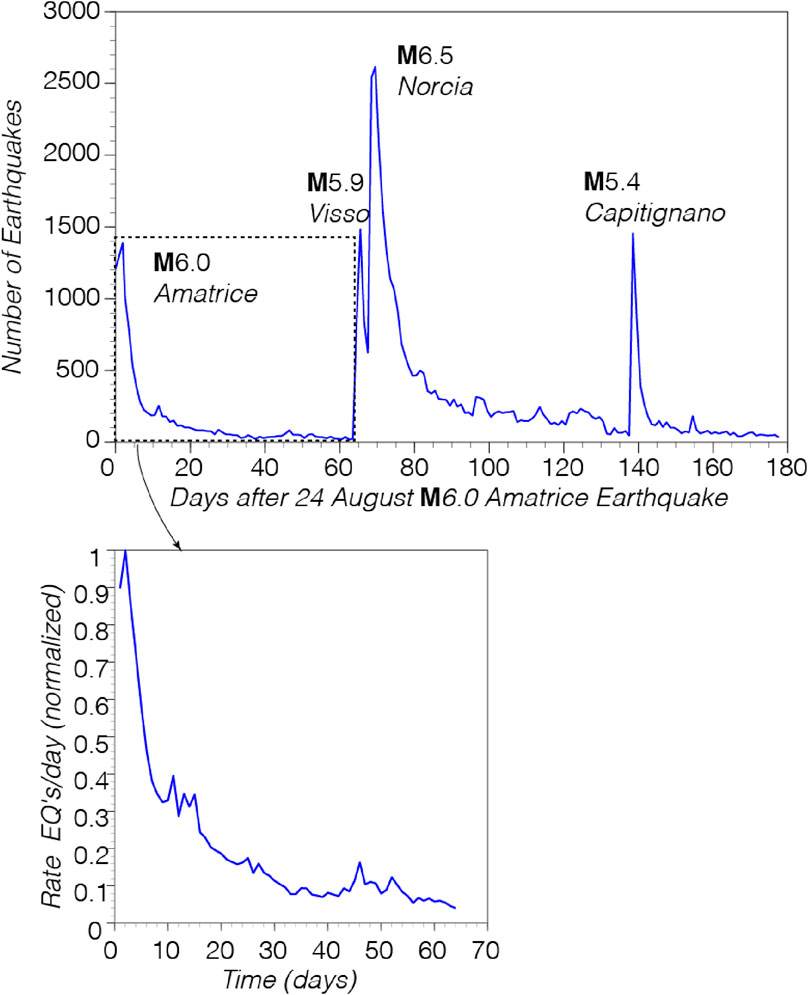
Figure 4. Daily earthquake numbers vs. time during the 2016 multi-mainshock sequence in the Central Apennines region of Italy from the high-resolution catalog by Tan et al. (2021). Inset shows the normalized aftershock rate during the first 64 days of the sequence after the first mainshock (Amatrice M6.0) that we fit to physics-based models of Omori’s law.

Fluid diffusion triggering is observed to be time dependent, and Nur and Booker (1972) developed an expression based on dislocation models in a porous medium as

$\frac{dN}{dT}=\frac{1}{\mathrm{\Omega }}{\int }_V\frac{\partial P}{\partial t}dV(2)$

Where P is pore fluid pressure, V is volume and $\mathrm{\Omega }$ is a constant. Malagnini et al. (2012) derived an expression for 1-D fluid diffusion under a steady state fluid pressure change based on the Nur and Booker (1972) relation as

$\frac{dN}{dT}=\frac{1}{\alpha }\frac{\left(P_0-P_1\right)}{2\sqrt{\pi D{t}^3}}{\int }_0^{\infty }xexp\left(-\frac{x^2}{4Dt}\right)dx=\frac{\left(P_0-P_1\right)\sqrt{D}}{\mathrm{\Omega }\sqrt{\pi }}\frac{1}{\sqrt{t}}(3)$

which implies that

$\frac{dN}{dT}\propto \frac{1}{\sqrt{t}}(4)$

Thus, the rate of fluid diffusion triggered aftershocks differs from the Omori-law time dependence of

$\frac{dN}{dT}\propto \frac{1}{t}(5)$

meaning that fluid diffusion may need to be accompanied by other aftershock-generating mechanisms to achieve Omori time dependence.

Cascades of secondary aftershock triggering can have important effects on the Omori decay after a mainshock. They create multiple series of peaks and decays that overprint the primary decay curve and scale with the magnitude of each aftershock (e.g., Ogata, 1998; Helmstetter and Sornette, 2002; Ziv, 2003; Ouillon and Sornette, 2005; Hainzl and Marsan, 2008). We use a randomized scaling term to fit secondary aftershock triggering because, while the rate of triggered events by the mainshock is predictable, the magnitudes of these events are not. This is an issue because larger aftershocks can trigger enough secondary aftershocks to significantly perturb the aftershock rate curve at unpredictable magnitudes within a sequence.

Putting the three terms together (Equations 3–5) and combining constant terms results in a nonlinear mixed effects problem as

$\frac{dN}{dT}=\left[\frac{r_{ref}}{\left(\Delta -1\right)\left(\exp \left(\frac{-t}{f}\right)\right)+1}\right]+\left[\frac{D}{\sqrt{t}}\right]+c\left(R^{0,1}t\right)(6)$

where t is time. The first term is the static and/or dynamic triggering rate, with r_ref being the reference (background) steady state seismicity rate. We treat r_ref as an unknown constant because the high-resolution catalog contains only ∼10 days of pre-mainshock observations, which is not long enough to constrain the background rate. We simplify the static stress change term $\mathit{exp}\left(\frac{-\Delta \tau }{a\sigma }\right)$ from Equation 1 as an unknown constant $\Delta$. The value f is the aftershock duration, which is constant. The second term is fluid diffusion triggering, and we apply an unconstrained constant D that represents diffusivity (Malagnini et al., 2012). The third term is the secondary triggering term with an unconstrained scaling constant c multiplied by a random number generator ranging between 0 and 1 (R^0,1). Our philosophy is to allow unconstrained ranges of values for free parameters to minimize bias, and to see if there are consistent trends in the results that can teach us about the underlying physics of Omori’s law. Of particular interest to us is the relative contributions between static stress triggering with Rate/State decay, fluid diffusion, and secondary triggering, allowing for the possibility that one or more terms might have ∼ zero contributions to solutions that match the observed aftershock decay curve with minimum RMS (root mean square) misfits.

4 Fitting an observed aftershock sequence with nonlinear regression

We use two regression approaches for fitting Equation 6 to an observed aftershock sequence, which in this case is the 64-day sequence after the 24 August 2016 M6.0 Amatrice earthquake up to and just prior to the 26 October 2016 M5.9 Visso and 30 October 2016 M6.5 Norcia mainshock earthquakes (Figure 4). We are fitting the high-resolution earthquake catalog of the 2016 Central Apennines, Italy earthquake sequence by Tan et al. (2021) that is complete to M_L>0.3 (M > 1.04). It is important to have as complete a catalog as possible to best represent Omori’s law because many smaller events can be undetected, especially during the earliest parts of the sequence when so many low-magnitude aftershocks are occurring that it can be difficult to resolve all of them.

Our hypothesis is that there is a mix of at least three physical causes of aftershocks that operate simultaneously. We thus have four unconstrained parameters to solve for in the equation for combined physical models of Omori’s law (Equation 6). The first method we use is a simulated annealing regression (Kirkpatrick et al., 1983; Černy, 1985) to find minimum RMS misfits to the observed sequence. Minimizing RMS error is a nonlinear and multivariable optimization procedure because the observed and theoretical decay curves (Equation 6) are nonlinear functions in time. Simulation of the observed curve is begun by using a stochastic sampling method for four free parameters. It starts from a random initial state and continues until a maximum of one million steps have been taken to minimize the RMS misfit between the model and the observed curve (Figure 4). All parameters are completely unconstrained in the simulated annealing regression and can be negative or positive, which can mean over or under predicting aftershock rates.

The underdetermined nature of the problem requires multiple iterations, so we calculate groups of 100 solutions minimized over one million attempts, which are then sorted for the lowest RMS misfit. Parameter values form the lowest RMS solution are then used as a starting point to explore neighboring points for better fits by perturbation within ±20% of their values. We allow those that increase the objective by returning higher RMS misfits to avoid trapping in local minima. Finally, the solutions are again refined by perturbing parameters within ±10% of their values and are limited to solution parameters that have lower RMS misfits than the input values. The compute cost is low enough that no cooling schedule is needed, which is sometimes used in simulated annealing to begin restricting the solution space to reduce the computational load. We run 1,000 independent regressions following the above-described steps to reasonably explore the solution space, and to identify trade-offs between parameters. We show the best fit solution, and the disaggregation of the three components from Equation 6 in Figure 5. This solution shows the contributions of physical models to be 114% static stress/Rate-State triggering, 9% fluid diffusion and −23% secondary triggering. We achieve low RMS misfits because the random secondary triggering term enables fitting to rate fluctuations associated with higher magnitude aftershocks; these fluctuations are not noise, but are an important part of the overall signal (e.g., Ogata, 1998; Helmstetter and Sornette, 2002; Ziv, 2003; Ouillon and Sornette, 2005; Hainzl and Marsan, 2008).

Figure 5

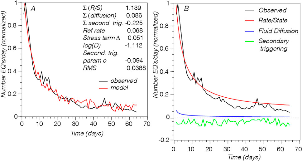
Figure 5. (A) Best fit model to observed by simulated annealing regression. Summed contributions from the three terms in Equation 6 are given, as well as the four free parameter values. In (B) the three weighted models are disaggregated so that each of their effects on the model fit can be seen.

We employ a second regression to test if there is method dependence on the results. We use a local interior-point optimization method for each of 1,000 random realizations of the secondary triggering term to minimize misfit to Equation (6). Interior-point regression involves a gradient search method (Forsgren et al., 2002; Boyd and Vandenberghe, 2004) that achieves optimization by going through the middle of a solid (e.g., convex hull) defined by the constraints rather than around its surface. The constraints together with the objective function (minimizing misfit) are combined using a logarithmic barrier function with the necessary Karush-Kuhn-Tucker (KKT) conditions. The nonlinear system of equations is then solved using Newton’s method. Interior-point implementations rely heavily on very efficient code (e.g., Cholesky decomposition) for factoring sparse symmetric matrices. Convergence for the interior-point method is determined by an augmented Lagrangian merit function (Birgin and Martínez, 2014). The interior-point method differs slightly from our application of the simulated annealing regression because the Rate/State reference rate (r), parameter (Δ), and diffusivity constant (D) are subject to positivity constraints.

We found that regularization was required for the interior-point approach to get low misfit solutions. This is the process of adding an additional constraint to the model to reduce its complexity by forcing certain predictor variables to have a smaller impact on the outcome or, no effect at all. We use LASSO (Least Absolute Shrinkage and Selection Operator) (Tibshirani, 1996) to help with feature selection and reduce the complexity of the model. It does this by regularizing the coefficients of each predictor variable, meaning it applies an L1 penalty for large coefficient values to bring them down to a size that is more manageable. This helps overall model accuracy by reducing the number of variables used while improving predictive power. LASSO can set the coefficient of some predictors toward zero, effectively eliminating them from the model. This helps to reduce complexity further and improve interpretability by reducing the number of variables included in a model.

As an alternative to using independent random variables for the secondary triggering term as given in Equation 6, the interior point algorithm also applied 1,000 realizations of an Ornstein-Uhlenbeck (O-U) random walk. The O-U random walk has random variations from a central expectation (zero for the secondary triggering term) that grow with time, and a restoring force that pulls values back toward that expectation (reversion parameter) that controls the dominant period of random fluctuations. We experimented with different reversion values to minimize cumulative RMS misfits. We show the best fit solution in Figure 6, which shows the relative contributions of physical models to be ∼120% static stress/Rate-State triggering, and −20% secondary triggering, with fluid diffusion triggering being effectively zero. The best-fit solutions from the interior point methods come from applying independent random variables for the secondary triggering term, whereas applying the O-U random walk to solutions causes consistently larger RMS misfits (see Supplementary Figure S2).

Figure 6

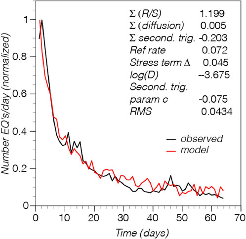
Figure 6. Best fit model to observed by interior point regression. Parameter values and sums from Equation 6 are given.

5 Results

We find multiple regression solutions with varying RMS misfits. We calculate 1,000 regressions with each method to understand the relative contributions to the overall model from each term representing a physical model. We find the contributions by summing up the number of predicted earthquakes made by each term and dividing that number by the total prediction of all three terms. In Figure 7 we show distributions of the relative contributions of each of the three terms in Equation 6. The range of contributions from both methods are remarkably consistent (Figures 7A,B) with distribution means and standard deviations that are nearly the same, with the Rate/State contribution mean of 1.170 for the simulated annealing regression vs. 1.169 for the interior point, with standard deviations of 0.064 and 0.063. For the secondary triggering term, the means are the same at −1.19 with standard deviations of 0.059 and 0.063. The fluid diffusion distributions are non-Gaussian. In general, the Rate/State model alone overpredicts the aftershock rate by ∼0–30%, while secondary aftershocks cause a negative contribution ranging between ∼0 and 30%, with a fluid diffusion contribution ranging from ∼0 to 20%. These results come from very different regression methods, implying that this may be a necessary outcome based on the how the mixed effects problem was posed in Equation 6, as well as our choice of the observed sequence. Additionally, Rate/State parameters can be distance dependent (e.g., Page et al., 2024), meaning that applying a fixed set of parameters for the entire sequence could cause misfit. Most aftershocks of the M6.0 Amatrice are contained within a 25 km radius of the mainshock (Figure 3A).

Figure 7

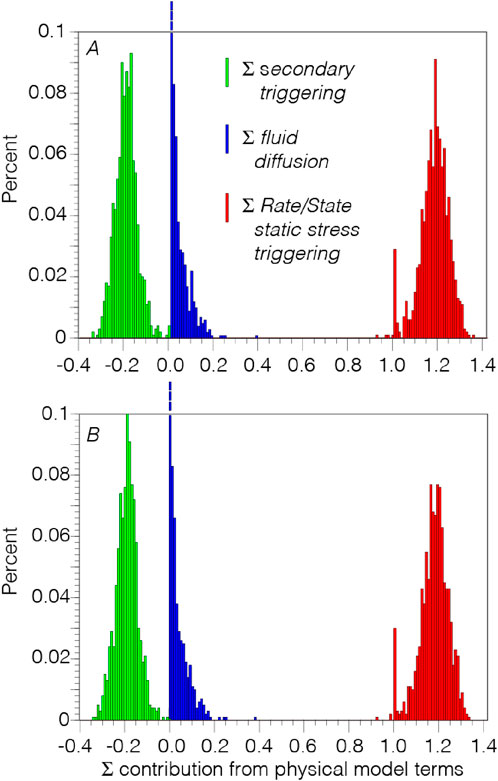
Figure 7. (A) Distributions of the sum contribution to predicted number of earthquakes from the Rate/State model (red histogram), the fluid diffusion model (blue histogram), and secondary triggering (green histogram) for random secondary triggering using the simulated annealing regression. In (B) the same information is shown from the interior point regression. The results from both regression models are similar.

While the two regression methods show very similar distributions of relative physical-model contributions, we find that the distributions of RMS misfit differ (Figure 8) between methods. There is overlap but the interior point regressions tend to have higher misfit values than do the simulated annealing regressions.

Figure 8

Figure 8. Histogram plots show the distributions of RMS misfits for 1,000 solutions from simulated annealing (red columns) and interior point (blue columns) regressions. In general, these plots show a wide range of possible values, but the most frequent values in the weighting parameters correlate with the lower RMS misfits identified in Figure 6.

We explore further to see if there are characteristic sets of parameters that cluster in a lower RMS state, which might lead us to further conclusions about the relative influence of different physical models for Omori’s law. We plot the relationships between the Rate/State static stress change term, secondary triggering term, RMS misfit, and number of solutions for both regression methods (Figure 9). These plots reveal that the most frequent solutions are not associated with the lowest RMS misfits.

Figure 9

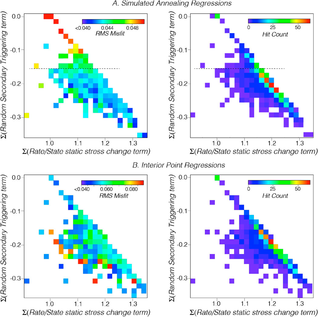
Figure 9. (A) Simulated annealing regression results: Left side shows a plot of summed contribution from Rate/State static stress triggering vs. the summed contribution from random secondary triggering vs. RMS misfit. Cooler colors show lower RMS values. The right side has the same axes except the relative frequency of solutions are colored with the summed number of solutions shown as a hit count. In (B) the same results are shown for the Interior Point regression. The frequency of solutions is very similar to the simulated annealing results (Figure 7), but the RMS misfit distributions are different.

We plot each parameter against RMS misfit for both regressions (Figures 10, 11) in isolation to determine if there are any weights or parameter values that have relatively stronger influences on fitting the observed aftershock sequence. We do not find what appear to be functional relationships between the free parameters and RMS misfits when they are isolated. We show linear regression fitting to the broadly scattered data for reference, but the data are not related through linear functions. We note that the simulated annealing regression results show parameters that are more scattered as function of RMS misfit, whereas the interior point values are more tightly clustered.

Figure 10

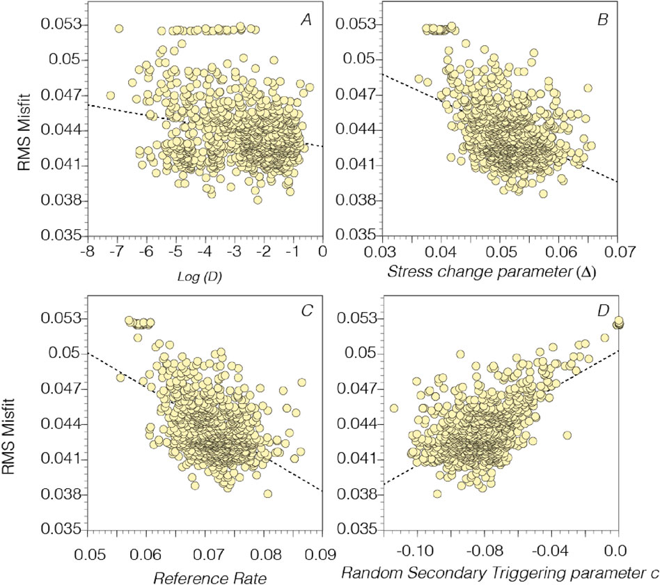
Figure 10. Plots of 1,000 simulated annealing regression parameter value results vs. RMS misfit. In (A) the log of the Diffusion parameter (D) is plotted with a simple linear regression applied that does not show a significant relationship vs. RMS. In (B) the stress change parameter (Δ) in the Rate/State expression (Equation 6) is plotted that shows a slight regression relationship. In (C) the reference rate term (r_ref) in the Rate/State expression (Equation 6) is plotted that also has a possible inverse relationship vs. RMS. In (D) it appears that the random secondary triggering parameter (c) seems to yield lower RMS values when c is more negative.

Figure 11

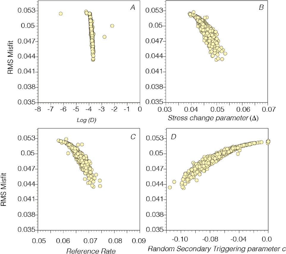
Figure 11. Plots of 1,000 interior point regression parameter value results vs. RMS misfit. Generally, the interior point results vs. RMS misfit are more tightly clustered than the simulated annealing regression results (Figure 10). The apparent relationships between parameter values vs. RMS have similar trends vs. RMS as do the simulated annealing regressions (Figure 10).

We find that all solutions from both regressions for the c parameter in the random secondary triggering term of Equation 6 yield negative values. It is the only parameter to have negative values amongst those that have no positivity constraints (positivity is limited to weighting the Rate/State reference rate (r), Rate/State parameter (Δ), and the diffusivity constant (D) in only the interior point method). Thus, because of the consistently negative c parameter in our solutions, the third term in Equation 6 is always subtracted from the first two. We provide a physical explanation of this in a later section of the paper.

We plot parameters as histograms (Figures 12, 13) that enable us to identify the most frequent values. If there is more than one peak on the histograms, then we have a suggestion of a tradeoff between parameters. We find that the same tradeoffs that were evident in Figure 7 are also seen in the histogram plots, between weighting of the Rate/State and secondary triggering components.

Figure 12

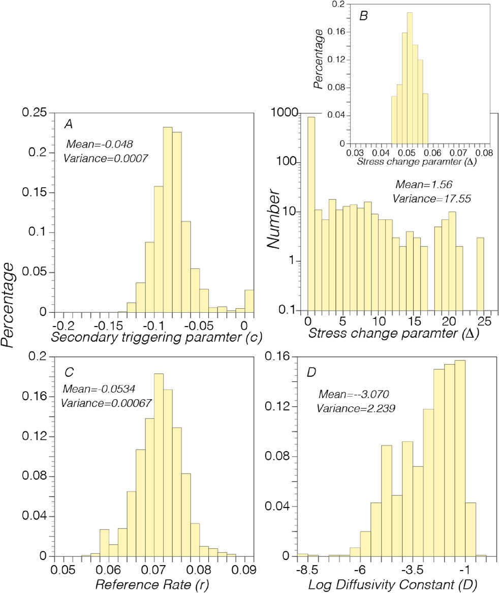
Figure 12. Distributions of free parameters from 1,000 simulated annealing regressions fitting Equation 6 to the observed aftershock sequence. The secondary triggering parameter (c), stress change parameter (Δ), and the reference rate (r_ref) appear to be approximately normally distributed. The distribution of the Log diffusivity (D) appears consistent with the observed range for faults and intervening rock (with Log(D) ranging from −1 to −5 (e.g., Brodsky and Saffer, 2020). The stress change parameter Δ (shown in panel b) has a higher variance with the majority of values ranging between 0.04–0.06 (see inset panel), though there are some values that reach as high as 25.

Figure 13

Figure 13. Distributions of free parameters from 1,000 interior point regressions fitting Equation 6 to the observed aftershock sequence. The parameters appear are more narrowly distributed than the simulated annealing values. The distribution of the Log diffusivity (D) is mostly consistent with the observed range for faults and intervening rock (with Log(D) ranging from ∼10⁻¹ to 10⁻⁵ (e.g., Brodsky and Saffer, 2020).

5.1 Overfitting?

We attempt to fit the first 64 days of the observed Amatrice aftershock sequence (Figure 4) as closely as possible using Equation 6, including small perturbations in aftershock rates. In machine learning there can be issues when fitting observed training data too closely because matching noise in the data can yield parameter values that cannot be generalized for prediction. Here we are not trying to find universal parameter values, but instead are interested in the relative roles of different physical processes involved in a single sequence. Additionally, if a given aftershock sequence is complete above a magnitude threshold, then we can expect that temporal fluctuation is not measurement error or noise intrusion but is instead the result of physical processes. Indeed, we can show that daily rate fluctuations are a result of the largest magnitudes of events and their secondary aftershocks occurring in each bin by comparing against daily moment sums (Figure 14). We have chosen to fit these rate fluctuations using a random function because, while the overall rate decay is predictable, the distribution of higher magnitude aftershocks that provoke rate changes is less so, as we discuss in the next section.

Figure 14

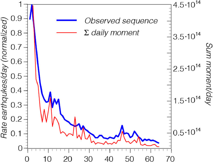
Figure 14. Comparison between observed aftershock sums in daily bins and daily moment sums indicate the effects of secondary earthquake triggering and their attendant aftershocks (e.g., Ogata, 1998; Helmstetter and Sornette, 2002; Ziv, 2003; Ouillon and Sornette, 2005; Hainzl and Marsan, 2008).

6 Explanation of results and parameter values

In this section we discuss two initially surprising results that are consistent across both regression methods. These are: (1) the uniformly negative c parameter values that scale the random secondary triggering factors of Equations 6, and (2) The relatively low weighting of fluid diffusion processes in fitting the observed aftershock sequence including near-zero weighting from the interior point algorithm, despite independent observations of these processes in the Apennines (Malagnini et al., 2012; Albano et al., 2019; Chiarabba et al., 2020; Malagnini et al., 2022). These results make sense to us upon reflection as described below.

6.1 Negative secondary triggering parameter

In our formulation, the exponential decay of aftershocks with time can be attributed to the declining array of nucleation zones in Rate/State theory, the diffusive nature of pore fluid pressure changes, and the occurrence of the aftershocks themselves and their secondary triggering. The uniform negative solutions for the random triggering parameter c are consistent with aftershocks decreasing an additional net differential stress state over time. According to static stress changes, each earthquake (including the mainshock) during the sequence creates volumes where the differential stress state is increased and decreased. Earthquakes are the response to the gradual increase in tectonic stress on faults that accumulates because of plate motions (e.g., Reid, 1910), and can be triggered if they are close to failure. While each aftershock can trigger others, they remove more stress than they create (Figure 15). We expect that the region under the influence of the mainshock and aftershocks will have a lower stress state than existed before they happened. In this way, the occurrence of aftershocks is a self-extinguishing process that must be subtracted from the exponential theoretical decay curves to most accurately fit observed sequences.

Figure 15

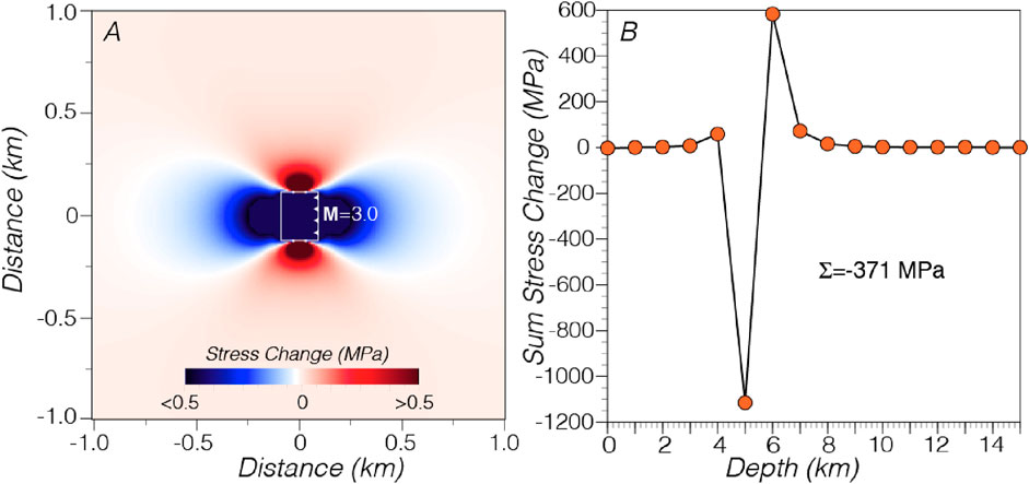
Figure 15. In (A) we simulate the stress change from a M3 within a 5 km cube. We then sum up the cumulative stress change within the cube (B), quantifying the sum of the stress change volume and verifying that it is indeed negative, which supports the regression solutions that are uniformly negative for the secondary triggering term.

It is abundantly clear that larger aftershocks and their associated secondary aftershocks do temporarily increase the total number of events as can be seen in the complete Amatrice series (Figure 4), where larger (M > 3.5) earthquakes cause significant temporary rate increases. We used a random distribution to include secondary earthquake triggering, meaning that we assume that the ratio of larger magnitude events to smaller ones is constant. In other words, we are assuming that the b-value is relatively constant throughout the sequence. The b-values vs. time in the Amatrice aftershock sequence was measured by Van der Elst (2021) who noted using what is called the β+ estimate, that the “b-value drops significantly after the first M6.2 earthquake in August but shows only a gradual increase and recovery after the final M6.6 earthquake in October.” Additionally, Mitsui (2024) noted that “Our findings indicated that the estimates produced by the b-positive method showed negligible variation between the 10-day and 1000-day aftershock periods (correlation coefficient of 0.95)”. This was found by Davidsen and Baiesi (2016), who noted self-similarity and that “the GR relation for triggered events needs to be modified if only triggered events over short time intervals are considered.”

The regression methods, while providing good overall fits, are not able to capture the initial rate increase spikes caused by secondary triggering from aftershocks of equal or greater magnitude as the mainshock. However, the methods do capture smaller spikes and the broader net decrease in aftershocks caused by reduced stress in the crust from the occurrence of thousands of earthquakes. We note that the very large (M > 5) aftershocks/mainshocks within the Amatrice sequence all occurred just at the edge of static stress change influence (Figure 3), implying that the physical processes driving the largest secondary events may be spatially more distinct from the initial aftershock decay of the initiating M6 Amatrice shock.

6.2 Low fluid diffusion weighting, and near-zero weighting from the interior point regression

Given the high pore fluid pressure that exists in the Apennines (e.g., Bonini, 2007), we were initially surprised that the regressions were returning such low weighting on fluid induced aftershock triggering following the Amatrice earthquake. There are however factors associated with fluid diffusion that likely mute their overall contributions to an Omori-law aftershock sequence that is extensive in time and space.

One factor we note is somewhat dependent on our regression methods. We find that the fluid diffusion term in the interior point regression method is weighted at ∼ zero, which is much lower than the simulated annealing regression, which has values up to 20% (Figure 7). This appears to be a result of regularization that is required for convergence in the interior point regression. Regularization seeks a smoother fit by minimizing parameters of lesser influence on the solution that could be interpreted as noise. The LASSO regularization applied in the interior point method seeks to essentially zero out parameters of low influence on the solutions, which explains the different outcomes in weighting fluid diffusion.

While there are methodological reasons for low weighting of fluid diffusion, there are also physical reasons. Previous modeling of diffusion processes within the Central Apennines indicate that the durations of the fluid pulses are short, being limited to 10 days or less (Figure 2) (Malagnini et al., 2012; Malagnini et al., 2022). Thus, they might not strongly influence the full 64-day-long sequence that we are fitting. Additionally, there are spatial constraints associated with high-pressure fluids such that they can be trapped within linear fault zones, or deep beneath the brittle crust in horizontal decollements (e.g., Bonini, 2007). Malagnini et al. (2012) noted that a diffusion signal could only be identified in a limited area where seismicity was migrating across a fault plane. Thus, given the massive number of small earthquakes (∼350,000 with M ≥ 1.04; Tan et al., 2021) that were broadly distributed temporally and spatially across the region following the Amatrice shock, the fluid diffusion signal is likely masked because of spatial and temporal limitations. Though in some cases fluid diffusion can be a dominant factor in seismicity rates (e.g., Miller, 2020; Jia et al., 2020). We did investigate a shorter duration catalog (8 days after the Amatrice mainshock and did find a larger proportion (0.356) as compared with of fluid diffusion triggering than we found using the full sequence up to the Visso shock (0.086). However, as we note in Supplementary Figure S2, the shorter sequence we analyzed is noisier and lacks the curvature we observe in longer sequences, diminishing our confidence in the fit to competing parameters.

6.3 Covariance

We computed a covariance matrix, which shows the potential tradeoffs between sets of parameters used in the regressions (Figure 16). Each parameter is also plotted against all the others (Figure 16). We note that, for the most part, the associations between parameters show relatively small values with absolute values less that 0.08 (Figure 16). The exception is the relationship between the fluid diffusion parameter (log(D), where D is a diffusivity constant) and the stress change parameter Δ), which has a covariance value that is two orders of magnitude higher than the combination of the other variables. When these two parameters are plotted against one another, there is a wide semi-horizontal spread (Figure 16), which may imply that these two parameters are more poorly constrained than the others.

Figure 16

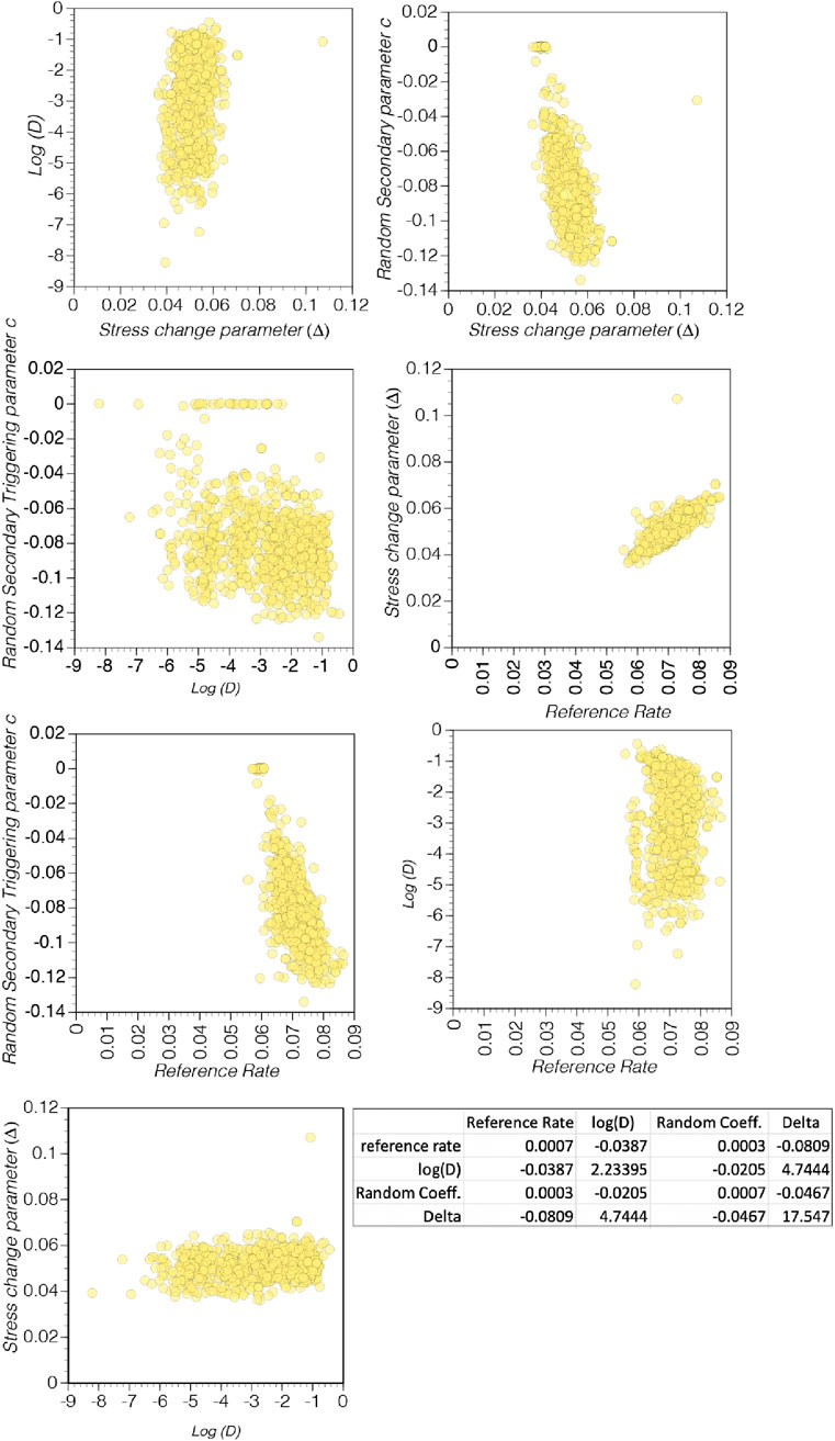
Figure 16. Plots of each variable from Equation 6 against all other variables. These plots identify variable covariance, which would be evident if there is an identifiable trend where there is an apparent functional relationship. The strongest example of this is the plot of reference rate vs. the stress change parameter Δ.

7 Conclusions

We apply two regression methods towards fitting an aftershock sequence to an equation that represents three physical models/concepts for earthquake triggering to understand the relative influences of: (1) static/dynamic stress changes from the mainshock, (2) fluid diffusion triggering, and (3) the random magnitude distribution vs. time amongst secondary triggering by aftershocks. There are four unconstrained parameters in Equation 6, which combines the three physical model terms. These are a reference seismicity rate, a static stress change term, a fluid diffusivity term, and a scaling constant for random secondary triggering. These four constants are solved by minimizing misfit to the first 64 days of aftershocks following the 24 August 2016 M6.0 Amatrice mainshock (Figure 4). We calculate 1,000 solutions from each regression method and find some consistent patterns amongst the solutions.

In all solutions the Rate/State model alone overpredicts the aftershock rate by 100%–130%, which is balanced by the random secondary triggering model which underpredicts by 0% to −30%. The fluid diffusion model predicts a 0%–20% contribution. Both regressions methods we used returned very similar and consistent results (Figure 7), including negative scaling factors for secondary triggering that appears to be required to fit the observed sequence that were not imposed. We conclude this is a necessary subtraction because while each earthquake that follows the mainshock triggers subsequent aftershocks, the net effect of each of them is to remove stress from the crust, leading to a self-extinguishing process (Figure 15).

Fluid diffusion triggering is consistently weighted low in both regression methods despite evidence that it is an important process in the Apennines (e.g., Bonini, 2007; Malagnini et al., 2012; Albano et al., 2019; Chiarabba, et al., 2020; Malagnini et al., 2022) (Figures 2, 3). We conclude that this is because diffusion processes are limited in time and space and thus do not have a strong signal over a long aftershock sequence.

Unaddressed by our regressions are the physical causes of secondary triggered earthquakes that each have their own Omori Law sequences that contribute to the overall signal. We have modeled this as rate effects from a uniform aftershock magnitude distribution (Figure 15b) that is subtracted from the expected sequence of the primary mainshock. We note here that there may be more opportunities for dynamic triggering within the sequence than from a single mainshock, to which roughly a third of the aftershocks have been attributed if fluid diffusion causes are neglected (e.g., Parsons, 2002; Hardebeck and Harris, 2022). These relatively small rate fluctuations that might be construed as noise are influential in our solutions such that they have as much as a 35% contribution to the overall aftershock time series distribution. This likely explains why statistical (e.g., Ogata, 1998; Ziv, 2003) or static stress change aftershock forecasts (Mancini et al., 2022) that update and account for secondary triggering are more accurate, which is a consideration for operational aftershock forecasting.

Results from regressions have enabled us to quantify ranges of the relative influences of physical processes on an aftershock rate distribution provided that the three models expressed in Equation 6 are correct and comprehensive. The primary conclusion that we reach is that any one physical model cannot alone fit the observed sequence as well as the combination of all three that we investigated (Figure 17). The concept of inverting for parameter values can be adapted to additional and/or alternative physical models in the future.

Figure 17

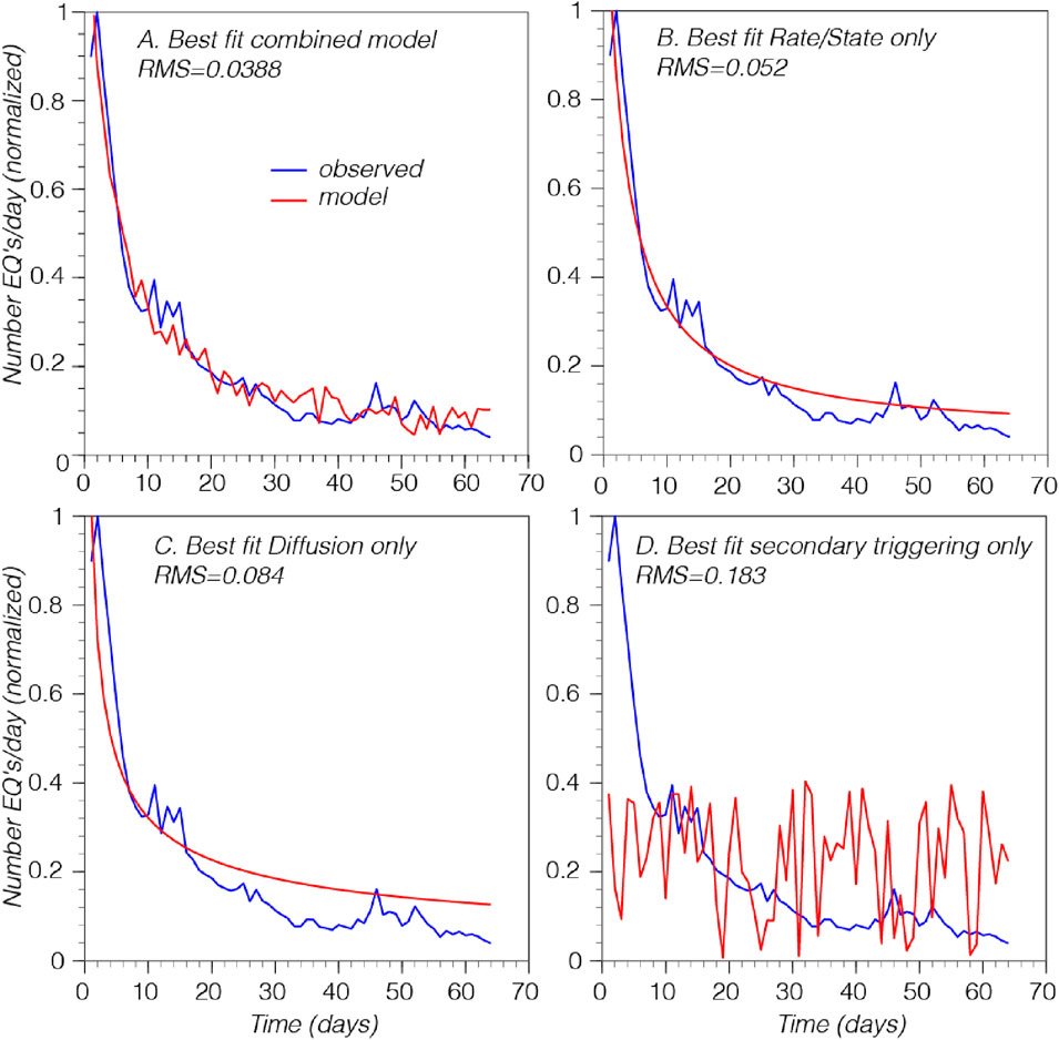
Figure 17. (A) The best fit model from the simulated annealing inversion based on all three terms of Equation 6. In (B) the best fit to observed to a Rate/State model only. In (C) and (D) the best fits applying only fluid diffusion and secondary triggering are shown. No individual model achieves as good a fit as the combined terms do.

Plain language summary

Aftershocks are most numerous immediately after a mainshock occurs, and we have known since Fusakichi Omori’s work in 1894 that they decay roughly as a function of 1/time. There are multiple observations/models for why this happens, and we are curious whether a mixture of these concepts is responsible, and if so, what is the relative importance of each. We distill these ideas into an equation of three terms: (1) a model of time-dependent friction on faults that causes a delayed response to stress changes instigated by the mainshock, (2) increased fluid pressure caused by the mainshock that pushes open fault walls enabling aftershocks to occur, and (3) aftershocks that can trigger additional aftershocks (secondary triggering). We use two different computational methods to find the best combinations of models that fit an observed aftershock sequence. We find that time dependent frictional responses to stress changes is the dominant cause of aftershocks as modified by the effects of secondary triggering. We find the impact of fluids in the crust is smaller for a long aftershock sequence but can be more important over shorter time periods, and that secondary aftershocks reduce stress in the crust and suppress continued seismicity.

Data availability statement

Publicly available datasets were analyzed in this study. This data can be found here: https://pmc.ncbi.nlm.nih.gov/articles/PMC9674631/

Author contributions

TP: Writing – review and editing, Conceptualization, Validation, Investigation, Formal Analysis, Software, Visualization, Writing – original draft. EG: Validation, Formal Analysis, Writing – review and editing, Writing – original draft, Methodology, Software, Conceptualization, Investigation. LM: Conceptualization, Methodology, Writing – original draft, Writing – review and editing, Investigation.

Funding

The author(s) declare that no financial support was received for the research and/or publication of this article.

Conflict of interest

The authors declare that the research was conducted in the absence of any commercial or financial relationships that could be construed as a potential conflict of interest.

Generative AI statement

The author(s) declare that no Generative AI was used in the creation of this manuscript.

Any alternative text (alt text) provided alongside figures in this article has been generated by Frontiers with the support of artificial intelligence and reasonable efforts have been made to ensure accuracy, including review by the authors wherever possible. If you identify any issues, please contact us.

Publisher’s note

All claims expressed in this article are solely those of the authors and do not necessarily represent those of their affiliated organizations, or those of the publisher, the editors and the reviewers. Any product that may be evaluated in this article, or claim that may be made by its manufacturer, is not guaranteed or endorsed by the publisher.

Supplementary material

The Supplementary Material for this article can be found online at: https://www.frontiersin.org/articles/10.3389/feart.2025.1619887/full#supplementary-material

References

Albano, M., Barba, S., Saroli, M., Polcari, M., Bignami, C., Moro, M., et al. (2019). Aftershock rate and pore fluid diffusion: insights from the amatrice-visso-norcia (italy) 2016 seismic sequence. J. Geophys. Res. Solid Earth 124, 995–1015. doi:10.1029/2018JB015677

CrossRef Full Text | Google Scholar

Biot, M. A. (1941). General theory of three-dimensional consolidation. J. Appl. Phys. 12, 155–164. doi:10.1063/1.1712886

CrossRef Full Text | Google Scholar

Birgin, E. G., and Martínez, J. M. (2014). Practical augmented lagrangian methods for constrained optimization. Philadelphia, Pennsylvania: Society for Industrial and Applied Mathematics.

Google Scholar

Bonini, M. (2007). Interrelations of mud volcanism, fluid venting, and thrust-anticline folding: examples from the externalnorthern apennines (Emilia-Romagna, Italy). J. Geophys. Res. 112, B08413. doi:10.1029/2006JB004859

CrossRef Full Text | Google Scholar

Boyd, S., and Vandenberghe, L. (2004). Convex optimization. Cambridge, UK: Cambridge University Press, 715.

Google Scholar

Brodsky, E. E., and Saffer, D. M. (2020). The hydraulic diffusivity of faults. Fall Meeting 2020: American Geophysical Union.

Google Scholar

Bullen, K. E., and Bolt, B. A. (1985). An introduction to the theory of seismology. 4th Edn. Cambridge University Press, 499.

Google Scholar

Černy, V. (1985). Thermodynamical approach to the traveling salesman problem: an efficient simulation algorithm. J. Optim. Theory Appl. 45 (1985), 41–51. doi:10.1007/bf00940812

CrossRef Full Text | Google Scholar

Chiarabba, C., Buttinelli, M., Cattaneo, M., and De Gori, P. (2020). Large earthquakes driven by fluid overpressure: the apennines normal faulting system case. Tectonics 39, e2019TC006014. doi:10.1029/2019TC006014

CrossRef Full Text | Google Scholar

Davidsen, J., and Baiesi, M. (2016). Self-similar aftershock rates. Phys. Rev. E 94, 022314. doi:10.1103/PhysRevE.94.022314

PubMed Abstract | CrossRef Full Text | Google Scholar

Dieterich, J. A. (1994). A constitutive law for rate of earthquake production and its application to earthquake clustering. J. Geophys. Res. 99, 2601–2618. doi:10.1029/93jb02581

CrossRef Full Text | Google Scholar

Dieterich, J. H., and Kilgore, B. D. (1996). Imaging surface contacts: power law contact distributions and contact stresses in quartz, calcite, glass, and acrylic plastic. Tectonophysics 256, 219–239. doi:10.1016/0040-1951(95)00165-4

CrossRef Full Text | Google Scholar

Ellsworth, W. L. (2013). Injection-induced earthquakes. Science 341, 1225942. doi:10.1126/science.1225942

PubMed Abstract | CrossRef Full Text | Google Scholar

Evans, D. M. (1966). The Denver area earthquakes and the Rocky Mountain Arsenal disposal well. Mt. Geol. 3, 23–26.

Google Scholar

Felzer, K. R., and Brodsky, E. E. (2006). Decay of aftershock density with distance indicates triggering by dynamic stress. Nature 441 (7094), 735–738. doi:10.1038/nature04799

PubMed Abstract | CrossRef Full Text | Google Scholar

Forsgren, A., Gill, P. E., and Wright, M. H. (2002). Interior methods for nonlinear optimization. SIAM Rev. 44 (4), 525–597. doi:10.1137/s0036144502414942

CrossRef Full Text | Google Scholar

Freed, A. M. (2005). Earthquake triggering by static, dynamic, and postseismic stress transfer. Annu. Rev. Earth Planet. Sci. 33, 335–367. doi:10.1146/annurev.earth.33.092203.122505

CrossRef Full Text | Google Scholar

Freed, A. M., and Lin, J. (2001). Delayed triggering of the 1999 hector Mine earthquake by viscoelastic stress transfer. Nature 411 (6834), 180–183. doi:10.1038/35075548

PubMed Abstract | CrossRef Full Text | Google Scholar

Hainzl, S., and Marsan, D. (2008). Dependence of the omori-utsu law parameters on main shock magnitude: observations and modeling. J. Geophys. Res. 113, B10309. doi:10.1029/2007JB005492

CrossRef Full Text | Google Scholar

Hardebeck, J. L., and Harris, R. A. (2022). Earthquakes in the shadows: why aftershocks occur at surprising locations. Seismic Rec. 2 (3), 207–216. doi:10.1785/0320220023

CrossRef Full Text | Google Scholar

Harris, R. A. (1998). Introduction to special section: stress triggers, stress shadows, and implications for seismic hazard. J. Geophys. Res. 103, 24347–24358. doi:10.1029/98JB01576

CrossRef Full Text | Google Scholar

Helmstetter, A., and Sornette, D. (2002). Diffusion of epicenters of earthquake aftershocks, Omori’s law, and generalized continuous-time random walk models. Phys. Rev. E Stat. Nonlinear, Soft Matter Phys. 66, 061104. doi:10.1103/PhysRevE.66.061104

PubMed Abstract | CrossRef Full Text | Google Scholar

Hill, D. P., Reasonberg, P. A., Michael, A., Arabasz, W. J., Beroza, G., Brune, J. N., et al. (1993). Seismicity in the Western United States remotely triggered by the M 7.4 landers, California, earthquake of June 28, 1992. Science 260, 1617–1623. doi:10.1126/science.260.5114.1617

PubMed Abstract | CrossRef Full Text | Google Scholar

Hubbert, M. K., and Rubey, W. W. (1959). Role of fluid pressures in mechanics of overthrust faulting: I. Mechanics of fluid-filled porous solids and its application to overthrust faulting. Geol. Soc. Amer. Bull. 70, 115–166. doi:10.1130/0016-7606(1959)70[115:ROFPIM]2.0.CO;2

CrossRef Full Text | Google Scholar

Jia, K., Zhou, S., Zhuang, J., Jiang, C., Guo, Y., Gao, Z., et al. (2020). Nonstationary background seismicity rate and evolution of stress changes in the changning salt mining and shale-gas hydraulic fracturing region, sichuan basin, China. Seismol. Res. Lett. 91, 2170–2181. doi:10.1785/0220200092

CrossRef Full Text | Google Scholar

Kato, A. (2024). Implications of fault-valve behavior from immediate aftershocks following the 2023 M_j6.5 earthquake beneath the noto peninsula, central Japan. Geophys. Res. Lett. 51, e2023GL106444. doi:10.1029/2023GL106444

CrossRef Full Text | Google Scholar

Kirkpatrick, S., Gelatt, C. D., and Vecchi, M. P. (1983). Optimization by simulated annealing. Science 220, 671–680. doi:10.1126/science.220.4598.671

PubMed Abstract | CrossRef Full Text | Google Scholar

Malagnini, L., Lucente, F. P., De Gori, P., Akinci, A., and Munafo’, I. (2012). Control of pore fluid pressure diffusion on fault failure mode: insights from the 2009 l’Aquila seismic sequence. J. Geophys. Res. 117, B05302. doi:10.1029/2011JB008911

CrossRef Full Text | Google Scholar

Malagnini, L., Parsons, T., Munafò, I., Mancini, S., Segou, M., and Geist, E. L. (2022). Crustal permeability changes inferred from seismic attenuation: impacts on multi-mainshock sequences. Front. Earth Sci. 10, 963689. doi:10.3389/feart.2022.963689

CrossRef Full Text | Google Scholar

Mancini, S., Segou, M., Werner, M. J., and Cattania, C. (2019). Improving physics-based aftershock forecasts during the 2016-2017 central Italy earthquake Cascade. J. Geophys. Res. Solid Earth 124, 8626–8643. doi:10.1029/2019JB017874

CrossRef Full Text | Google Scholar

Mancini, S., Segou, M., Werner, M. J., Parsons, T., Beroza, G., and Chiaraluce, L. (2022). On the use of high-resolutionand deep-learning seismic catalogsfor short-term earthquake forecasts: potential benefits and current limitations. J. Geophys. Res. Solid Earth 127, e2022JB02520. doi:10.1029/2022JB025202

PubMed Abstract | CrossRef Full Text | Google Scholar

Mikumo, T., and Miyatake, T. (1979). Earthquake sequences on a frictional fault model with non-uniform strengths and relaxation times. J. Int. 59 (3), 497–522. doi:10.1111/j.1365-246X.1979.tb02569.x

CrossRef Full Text | Google Scholar

Miller, S. A. (2020). Aftershocks are fluid-driven and decay rates controlled by permeability dynamics. Nat. Commun. 11, 5787. doi:10.1038/s41467-020-19590-3

PubMed Abstract | CrossRef Full Text | Google Scholar

Mitsui, Y. (2024). Stable estimation of the gutenberg–richter b-values by the b-positive method: a case study of aftershock zones for magnitude-7 class earthquakes. Earth Planets Space 76, 92. doi:10.1186/s40623-024-02035-2

CrossRef Full Text | Google Scholar

Morikami, S., and Mitsui, Y. (2020). Omori-like slow decay (p < 1) of postseismic displacement rates following the 2011 tohoku megathrust earthquake. Earth, Planets Space 72, 37. doi:10.1186/s40623-020-01162-w

CrossRef Full Text | Google Scholar

Moutote, L., Itoh, Y., Lengliné, O., Duputel, Z., and Socquet, A. (2023). Evidence of a transient aseismic slip driving the 2017 Valparaiso earthquake sequence, from foreshocks to aftershocks. J. Geophys. Res. Solid Earth 128, e2023JB026603. doi:10.1029/2023JB026603

CrossRef Full Text | Google Scholar

Nur, A., and Booker, J. R. (1972). Aftershocks caused by pore fluid flow? Science 4024, 885–887. doi:10.1126/science.175.4024.885

PubMed Abstract | CrossRef Full Text | Google Scholar

Ogata, Y. (1988). Statistical models for earthquake occurrences and residual analysis for point processes. J. Am. Stat. Assoc. 83, 9–27. doi:10.1080/01621459.1988.10478560

CrossRef Full Text | Google Scholar

Ogata, Y. (1998). Space-time point process models for earthquake occurrences. Ann. Inst. Stat. Mech. 50, 379–402. doi:10.1023/a:1003403601725

CrossRef Full Text | Google Scholar

Omori, F., and Coll, J. (1894). On after-shocks of earthquakes. Sci. Imp. Univ. Tokyo 7, 111–200.

Google Scholar

Ouillon, G., and Sornette, D. (2005). Magnitude-dependent omori law: theory and empirical study. J. Geophys. Res. 110, B04306. doi:10.1029/2004JB003311

CrossRef Full Text | Google Scholar

Page, M. T., van der Elst, N. J., and Hainzl, S. (2024). Testing rate-and-state predictions of aftershock decay with distance. Seismol. Res. Lett. 95, 3376–3386. doi:10.1785/0220240179

CrossRef Full Text | Google Scholar

Parsons, T. (2002). Global omori law decay of triggered earthquakes: large aftershocks outside the classical aftershock zone. J. Geophys. Res. 107 (B9), 2199. doi:10.1029/2001JB000646

CrossRef Full Text | Google Scholar

Parsons, T. (2005). A hypothesis for delayed dynamic earthquake triggering. Geophys. Res. Lett. 32, L04302. doi:10.1029/2004GL021811

CrossRef Full Text | Google Scholar

Parsons, T., and Velasco, A. A. (2009). On near-source earthquake triggering. J. Geophys. Res. 114. doi:10.1029/2008JB006277

CrossRef Full Text | Google Scholar

Parsons, T., Segou, M., and Marzocchi, W. (2014). The global aftershock zone. Tectonophysics 618, 1–34. doi:10.1016/j.tecto.2014.01.038

CrossRef Full Text | Google Scholar

Pollitz, F. F. (1992). Postseismic relaxation theory on the spherical Earth. Bull. Seismol. Soc. Am. 82, 422–453. doi:10.1029/97JB01277

CrossRef Full Text | Google Scholar

Pollitz, F. F., and Sacks, I. S. (2002). Sress triggering of the 1999 hector mine earthquake by transient deformation following the 1992 landers earthquake, bulletin of the seismological society of America. Bull. Seismol. Soc. Am. 92 (4), 1487–1496. doi:10.1785/0120000918

CrossRef Full Text | Google Scholar

Pranger, C., Sanan, P., May, D. A., Le Pourhiet, L., and Gabriel, A.-A. (2022). Rate and state friction as a spatially regularized transient viscous flow law. J. Geophys. Res. Solid Earth 127, e2021JB023511. doi:10.1029/2021JB023511

CrossRef Full Text | Google Scholar

Reid, H. F. (1910). The Mechanics of the earthquake, the California Earthquake of April 18, 1906, report of the State investigation Commission. Washington, D.C: Carnegie Institution of. p. 16–28.

Google Scholar

Richards-Dinger, K., Stein, R., and Toda, S. (2010). Decay of aftershock density with distance does not indicate triggering by dynamic stress. Nature 467, 583–586. doi:10.1038/nature09402

PubMed Abstract | CrossRef Full Text | Google Scholar

Ruina, A. L. (1983). Slip instability and state variable friction laws. J. Geophys. Res. 88 (10), 10359–10370. doi:10.1029/jb088ib12p10359

CrossRef Full Text | Google Scholar

Sammis, C. G., Smith, S. W., Nadeau, R. M., and Lippoldt, R. (2016). Relating transient seismicity to episodes of deep creep at parkfield, California. Bull. Seismol. Soc. Am. 106 (4), 1887–1899. doi:10.1785/0120150224

CrossRef Full Text | Google Scholar

Segou, M., and Parsons, T. (2018). Testing Earthquake links in Mexico from 1978 to the 2017M = 8.1 Chiapas andM = 7.1 Puebla Shocks. Geophys. Res. Lett. 45, 708–714. doi:10.1002/2017GL076237

CrossRef Full Text | Google Scholar

Segou, M., and Parsons, T. (2020). The Role of Seismic and Slow Slip Events in Triggering the 2018 M7.1 Anchorage Earthquake in the Southcentral Alaska Subduction Zone. Geophys. Res. Lett. 47, e2019GL086640. doi:10.1029/2019GL086640

CrossRef Full Text | Google Scholar

Shcherbakov, R., Turcotte, D. L., and Rundle, J. B. (2004). A generalized Omori's law for earthquake aftershock decay. Geophys. Res. Lett. 31 (11), L11613. doi:10.1029/2004gl019808

CrossRef Full Text | Google Scholar

Stein, R. S. (1999). The role of stress transfer in earthquake occurrence. Nature 402, 605–609. doi:10.1038/45144

CrossRef Full Text | Google Scholar

Tan, Y. J., Waldhauser, F., Ellsworth, W. L., Zhang, M., Zhu, W., Michele, M., et al. (2021). Machine-Learning-Based High-Resolution Earthquake Catalog Reveals How Complex Fault Structures Were Activated during the 2016–2017 Central Italy Sequence. Seismic Rec. 1, 11–19. doi:10.1785/0320210001

CrossRef Full Text | Google Scholar

Tibshirani, R. (1996). Regression shrinkage and selection via the lasso. J. Roy. Stat. Soc. Ser. B 58, 267–288. doi:10.1111/j.2517-6161.1996.tb02080.x

CrossRef Full Text | Google Scholar

Tung, S., and Masterlark, T. (2018). Delayed poroelastic triggering of the 2016 October Visso earthquake by the August Amatrice earthquake, Italy. Geophys. Res. Lett. 45, 2221–2229. doi:10.1002/2017GL076453

CrossRef Full Text | Google Scholar

Uidas, A. (1999). Principles of seismology. New York, NY: Cambridge Univ. Press, 475.

Google Scholar

Utsu, T., Ogata, Y., and Matsu'ura, R. S. (1995). The Centenary of the Omori Formula for a Decay Law of Aftershock Activity. J. Phys. Earth 43, 1–33. doi:10.4294/jpe1952.43.1

CrossRef Full Text | Google Scholar

van der Elst, N. J. (2021). B-positive:A robust estimator of aftershock magnitude distribution in transiently incomplete catalogs. J. Geophys. Res. Solid Earth 126, e2020JB021027. doi:10.1029/2020JB021027

CrossRef Full Text | Google Scholar

Velasco, A. A., Hernandez, S., Parsons, T., and Pankow, K. (2008). Global ubiquity of dynamic earthquake triggering. Nat. Geosci. 1, 375–379. doi:10.1038/ngeo204

CrossRef Full Text | Google Scholar

Yamashita, T. (1979). Aftershock occurrence due to viscoelastic stress recovery and an estimate of the tectonic stress field near the San Andreas fault system. Bull. Seismol. Soc. Am. 69 (3), 661–687. doi:10.1785/BSSA0690030661

CrossRef Full Text | Google Scholar

Zhang, X., and Shcherbakov, R. (2016). Power-law rheology controls aftershock triggering and decay. Sci. Rep. 6, 36668. doi:10.1038/srep36668

PubMed Abstract | CrossRef Full Text | Google Scholar

Ziv, A. (2003). Foreshocks, aftershocks, and remote triggering in quasi-static fault models. J. Geophys. Res. 108 (B10), 2002JB002318. doi:10.1029/2002JB002318

CrossRef Full Text | Google Scholar