Detrended fluctuation analysis based on best-fit polynomial

Introduction

In various systems in nature, a broad variety of signals present complex behaviour that can exhibit long-term persistence, such as DNA sequences, human gait, and weather records (Chianca et al., 2005). Long-term persistence is also commonly referred to as long-range correlation (LRC), which implies that there is non-negligible dependence between the present and all points in the past (Timothy et al., 2017). Many climatic observations show LRC (Jiang et al., 2015), which means past climate has a long-term effect on the future evolutionary trend of the climate system (Bartos and Jánosi, 2006). Quantifying the LRC is crucial for understanding the dynamics of the systems. If a time series is characterized by LRC, then its autocorrelation function decays by a power law, as $C\left(n\right)\sim n^{-\alpha }$, where n is the lag time and C(n) is the autocorrelation (Kantelhardt et al., 2001). Scaling exponent can be used to quantitatively describe the strength of LRC of a time series, which can be estimated by various methods, such as fluctuation analysis (FA), detrended fluctuation analysis (DFA) and rescaled range (R/S) analysis (Hurst, 1951; Peng et al., 1992; Peng et al., 1994).

Most signals from complex physical and biological systems are nonstationary and are embedded in various trends, which leads to difficulties in quantifying the LRCs of the signals. R/S and power spectral analysis can only be used for stationary time series. DFA shows an advantage over the conventional methods. DFA can systematically eliminate nonstationary trends by changing the order of polynomial fitting, and avoids the spurious detection of apparent self-similarities which may be an artefact of extrinsic trends (Kantelhardt et al., 2002). DFA has been widely applied in climate research, such as quantifying the LRC of climate systems (Zhao et al., 2017), evaluating the dynamic characteristics of climate system models (Blender and Fraedrich, 2003), and further the performance of climate system model. Zhao et al. (2021) investigated the LRC characteristics of global air temperature of 8 models from CMIP5, and indicated that four models perform better than the others over most regions of the global ocean. However, the nonlinear filtering properties involved with detrending in the DFA method may induce instabilities in the scaling exponent estimation (Kiyono and Tsujimoto, 2016).

Many studies managed to improve the DFA method by introducing different detrending techniques, such as the centered moving average (CMA) method (Ramirez et al., 2005), the modified detrended fluctuation analysis (MDFA) (Kiyono et al., 2005), detrended moving average (DMA) method (Arianos and Carbone, 2007), and orthogonal detrended fluctuation analysis (Govindan, 2020). Different methods show various advantages and limitations (Chen et al., 2005; He et al., 2011). DFA analysis based on empirical mode decomposition (EMD) performs better than the classic DFA when the time series is strongly anticorrelated (Qian et al., 2011). CMA performance is slightly superior to DFA (Shao et al., 2012). DMA method performs better than DFA for signals with scaling exponent between 0.2 and 0.8, while DFA performs better when the scaling exponent exceeding 0.8 (Xu et al., 2005). Numerical analysis shows traditional DFA still has advantages in some situations (Grech and Mazur, 2005; Bashan et al., 2008).

In this study, the traditional DFA and its modification were used to estimate the scaling exponents of LRC of time series produced by FFM. DFA methods are described and then the results of DFA with different polynomial order are presented. Next, the results of regular DFA and the alternative method are systematically compared. And then, the influence of time series length on the calculated results is investigated. In the end, the main conclusion of this study and a brief discussion are presented.

Methods

Detrended fluctuation analysis

DFA can be used to estimate the strength of the LRC in a time series (Peng et al., 1994; Hu et al., 2001). DFA is performed using the following steps:

(1) The anomalies of a time series {x(i), i = 1, 2, …, N} are first calculated, and then gradually accumulate to form a new time series {Y(i), i = 1, 2, …, N}.

(2) The profile Y(i) is separated into non-overlapping segments with equal length $\tau$. Considering statistical reliability, τ varies from 10 to N/4 (Kantelhardt et al., 2002) with the interval of 1 in this study.

(3) In each segment, the polynomial trend of order p is calculated and then eliminated from the segment to obtain the fluctuation time series. When p = 2, a 2nd-order polynomial function is used to fit the profile (DFA-2). DFA-6 uses a 6nd-order polynomial function. DFA-2 is used the most frequently among different DFA-n methods.

(4) The variance of all the fluctuation time series is averaged to obtain the mean variance fluctuation function $F_p\left(\mathrm{\tau }\right)$. If there is a power law relationship between $F_p\left(\mathrm{\tau }\right)$ and $\tau$, then

$F_p\left(\mathrm{\tau }\right)\sim {\tau }^{\mathit{\alpha }}(1)$

here, α is the scaling exponent. If α = 0.5, the time series is a random sequence without long-term persistence. If 0.5<α<1.0, the time series has long-term persistence. If 0<α<0.5, an anti-correlation exists in the time series.

Best-fit polynomial

We propose to use best-fit polynomial in step (3). In each non-overlapping segment, the trend of the time series is calculated by best-fit polynomial functions with the maximum order varying from 2 to k. Then the best-fit degree of a polynomial fit is selected by minimizing the chi-square method. However, there is a problem in determining the value of k. We performed two independent sets of tests to show the effect of polynomial order on the DFA results. In each group, 2000 time series with length of 20,000 were generated by Fourier-filtering method (Peng et al., 1991). The actual scaling exponents are 0.3 and 0.8, respectively. The box charts of the scaling exponents calculated by different DFA-n are shown in Figure 1.

FIGURE 1

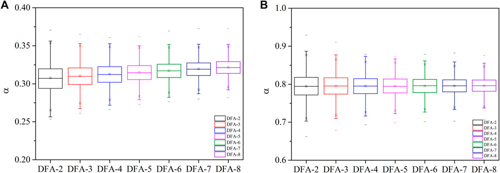
FIGURE 1. The box chart for DFA-n tests and the actual scaling exponents of the time series is 0.3 (A) and 0.8 (B).

For both group tests, the range of calculated scaling exponents decreases with polynomial order (Figures 1A,B). The minimum value of DFA-n results for time series of 0.3 increased apparently while the maximum value basically unchanged (Figure 1A). The median value of DFA-n results also showed an increasing trend with the order of polynomial functions in Figure 1A. In Figure 1B, the maximum value of DFA-n results decreased while the minimum value increased. Thus, the median value of DFA-n results varied little with order for time series with scaling exponents of 0.8. The median value error is more apparent for signals of 0.3 than those of 0.8 with the increase of n-order. In general, the range and median value of DFA-n results vary little for order varying from 6 to 8. Considering computational cost, the maximum order of the best-fit polynomial can be set to 6, and the minimum order is set to 1. DFA based on best-fit polynomial with the maximum order of 6 is described as DFA-BEST6 in this study.

Results

Comparison of DFA-2, DFA-6 and DFA-BEST6

The LRC exponents calculated by DFA-2, DFA-6 and DFA-BEST6 were compared in Figure 2. The actual scaling exponent of time series varies from 0.3 to 0.9 with an increment of 0.1 from test 1 to test 7. The 10,000 time series generated by the FFM method is used in each test. The sample size is 20,000 in each time series. The box chart shows the median, maximum, minimum and interquartile value of the estimated exponents for 10,000 time series (Figure 2). Results of DFA-2, DFA-6, and DFA-BEST6 can all characterize the LRC reliably. The range of scaling exponents calculated by the three DFA methods increases with the actual value. The range of the DFA-2 results are greater than those from DFA-6 and DFA-BEST6. The range of scaling exponents obtained by DFA-BEST6 is the smallest among the three methods. The median values of DFA-2 and DFA-6 are close to the actual values when the scaling exponent is greater than 0.5, while larger than the actual values when it is smaller than 0.5. For DFA-BEST6, the computed scaling exponents are close to the actual values in all tests, especially when the actual value is smaller than 0.5.

FIGURE 2

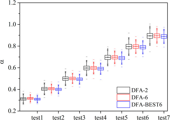
FIGURE 2. The box chart for results of DFA-2, DFA-6 and DFA-BEST6 methods for 10,000 time series.

Further comparison of the results from DFA-6 and DFA-BEST6 were shown in histograms (Figures 3A,B). The scaling exponents from DFA-BEST6 varied from 0.26 to 0.36, while the results from DFA-6 varied from 0.27 to 0.37. The percentage of scaling exponents from 0.29 to 0.32 calculated by DFA-BEST6 is 82.9%, while that calculated by DFA-6 is 70.5%. Results of DFA-BEST6 centred around 0.31 while those of DFA-6 centred around 0.32 (Figure 3A). For time series of 0.9, distributions of the results of DFA-6 and DFA-BEST6 are consistent and concentrated around the actual value, which shows better performance than the time series of 0.3 (Figure 3B). The percentage of scaling exponents between 0.86 and 0.92 from DFA-BEST6 is 83%, and that from DFA-6 is 82.6%. In general, the results of DFA-BEST6 are more concentrated around the actual value than DFA-6, which indicates better performance.

FIGURE 3

FIGURE 3. The histograms of scaling exponents simulated by DFA-6 and DFA-BEST6 for time series with actual scaling exponents of 0.3 (A) and 0.9 (B), respectively.

Traditional DFA and the alternative methods presented above all can successfully detect LRCs in signals well. DFA-BEST6 shows better performance than the other two methods statistically. In Figure 4 we show an example of a time series produced by FFM with a scaling exponent of 0.7. The result of DFA-BEST6 is equal to the actual value. However, the scaling exponent calculated by DFA-2 and DFA-6 are both 0.74, which is larger than the actual value. Both DFA-2 and DFA-6 have larger values of the root mean square fluctuation functions than DFA-BEST6, which indicates the variance of the results of DFA-BEST6 is smaller than those of DFA-2 and DFA-6.

FIGURE 4

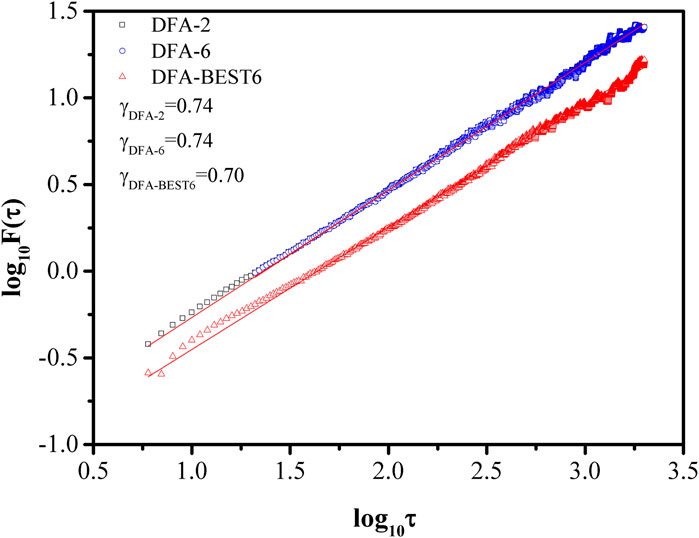
FIGURE 4. Fluctuation Function $\mathrm{F}\left(\tau \right)$ from the DFA-2, DFA-6, and DFA-BEST6 for time series with scaling exponent of 0.7. The black squares denote the results of DFA-2, blue circles denote DFA-6, and red triangles denote DFA-BEST6.

The 20,000 samples of time series used in Figure 4 are shown in Figure 5A, showing the stochastic character. In Figure 5B, the estimated trend Ys(i) (red lines) in DFA-2 shows discontinuous jumps at the end points of each window. For DFA-6, the estimated trend Ys(i) also shows discontinuous jumps at the end of each window (Figure 5C). However, the deviation of fitted trend from the cumulative anomaly in Figure 5C is smaller than that in Figure 5B. In contrast, the estimated trend in DFA-BEST6 shows continuous behaviour (Figure 5D). The deviation of fitted trend from the cumulative anomaly in DFA-BEST6 is the smallest among the three methods, which is consistent with the results in Figure 4.

FIGURE 5

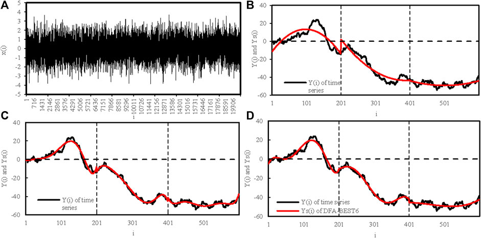
FIGURE 5. (A) time series with the length of 20,000, and the profiles Y(s) (black lines) and the fitted profiles Ys(i) (red lines) calculated by (B) DFA-2, (C) DFA-6, and (D) DFA-BEST6 method. The box size s = 200.

Influence of time series length

For time series with scaling exponent of 0.3, the scaling exponents calculated by DFA-2, DFA-6, and DFA-BEST6 are stable when the time series length approaches 1,000 (Figure 6A). The variance range of results of DFA-6 is smaller than those of DFA-2 and DFA-BEST6 when the time series length is greater than 1,000, and vice versa. For the time series of 0.9, the effect of the data length is less pronounced compared to the time series of 0.3. The calculated scaling exponents are stable when the time series reaches 500 (Figure 6B). The performance of DFA-BEST6 is better than those of DFA-2 and DFA-6 as the length of the time series increases.

FIGURE 6

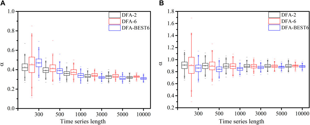
FIGURE 6. The box chart for results of DFA-2, DFA-6 and DFA-BEST6 tests for 2000 samples with data length varied from 300 to 10,000 and scaling exponents of (A) 0.3, (B) 0.9.

To quantify the degree of bias in the median exponents estimated from DFA-2, DFA-6 and DFA-BEST6. Relative error is calculated as follows: $\mathrm{E}=\frac{E_{est}-E_{act}}{E_{act}}*100$, where $E_{est}$ is the median exponent estimated by three methods and $E_{act}$ is the actual exponent of the long-range correlated data used in the analysis. E takes on a value zero if an approximation correctly characterizes the exponent. In Figure 7, we show the variation of E as a function of actual scaling exponent for DFA-2, DFA-6, and DFA-BEST6. For the short dataset containing 3,000 samples, the relative error of exponents estimated is about 6.9%, 14.7% and 6.2% for DAF-2, DFA-6 and DFA-BEST6, respectively (Figure 7A). For 20,000 samples, the exponents estimated form DAF-2 show a relative error of about 3.7% and those from DFA-BEST6 show a relative error of about 3.2%, whereas those from DFA-6 show a relative error of about 5.5% (Figure 7B). The relative error for the 20,000 samples is smaller than that for 3,000 samples, and results estimated from DFA-BEST6 are relatively more stable than other two methods.

FIGURE 7

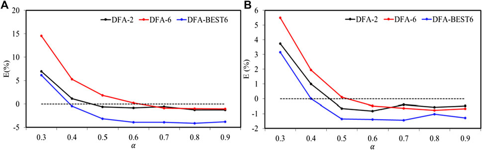
FIGURE 7. Relative error: the biases of the median of estimated exponents from the actual ones are shown for DFA-2, DFA-6 and DFA-BEST6 in (A) for 3,000 samples and in (B) for 20,000 samples.

Conclusion and discussion

In this paper, we introduce a variant of the DFA method using best-fit polynomial to characterize long-range correlations. By systematically comparing with the results of DFA-n (n = 2, 3,..., 8), we found the result of DFA-n with high order is better than that of low order when the scaling exponents is larger than 0.5. However, the improvement is slight when the order exceeds 6. Then the order of 6 is chosen as the highest order of the best-fit polynomial. The detrending procedure using n-order polynomial results in discontinuous jumps at the end points of each window, a property that may induce an increase in the estimation error.

A modification to the DFA is proposed in this study, which uses best-fit polynomial to detrend local trend in each segment. Numerical studies have shown that best-fit polynomial can effectively improve the bias at the end of each window. The proposed method performs as well as the traditional DFA method in estimating the scaling exponent when the exponents of the time series exceed 0.5. DFA-BEST6 characterizes the long-range correlations better than the original approach when scaling exponents are below 0.5. DFA-BEST6 can eliminate the external linearing trend as well as DFA-2 (see Supplementary Material). The estimation of the LRC reaches a stable state when the data length is larger than 1,000. The data length has a stronger effect on signals of smaller scaling exponents. DFA-BEST6 quantifies the LRC exponent with a relative error of about 6.2% for short datasets (3,000 samples) and a relative error of about 3.2% for long datasets (20,000 samples).

The results of this study have shown that a methodological improvement in DFA by modifying the detrending algorithm. Although DFA-BEST6 is able to improve the estimation of the scaling exponent, there is an overfitting phenomenon in the results, especially for signals with strong LRC. Moreover, this approach would require a considerably larger computational cost than regular DFA. These need further studies to improve the method.

Data availability statement

The raw data supporting the conclusion of this article will be made available by the authors, without undue reservation.

Author contributions

SZ and WH contributed to conception and design of the study. SZ organized the database and performed the statistical analysis. SZ wrote the first draft of the article. WH, YJ, YM, XX, and SW revised the article.

Funding

This research was supported by National Natural Science Foundation of China (Grant Nos. 41875120, 41975086 and 42175067).

Acknowledgments

The authors would like to thank the reviewers and editors for the beneficial and helpful suggestions for this manuscript.

Conflict of interest

The authors declare that the research was conducted in the absence of any commercial or financial relationships that could be construed as a potential conflict of interest.

Publisher’s note

All claims expressed in this article are solely those of the authors and do not necessarily represent those of their affiliated organizations, or those of the publisher, the editors and the reviewers. Any product that may be evaluated in this article, or claim that may be made by its manufacturer, is not guaranteed or endorsed by the publisher.

Supplementary material

The Supplementary Material for this article can be found online at: https://www.frontiersin.org/articles/10.3389/fenvs.2022.1054689/full#supplementary-material

References

Arianos, S., and Carbone, A. (2007). Detrending moving average algorithm: A closed-form approximation of the scaling law. Phys. A Stat. Mech. its Appl. 382, 9–15. doi:10.1016/j.physa.2007.02.074

CrossRef Full Text | Google Scholar

Bartos, I., and Jánosi, I. M. (2006). Nonlinear correlations of daily temperature records over land. Nonlinear process. geophys. 13, 571–576. doi:10.5194/npg-13-571-2006

CrossRef Full Text | Google Scholar

Bashan, A., Bartsch, R., Kantelhardt, J. W., and Havlin, S. (2008). Comparison of detrending methods for fluctuation analysis. Phys. A Stat. Mech. its Appl. 387, 5080–5090. doi:10.1016/j.physa.2008.04.023

CrossRef Full Text | Google Scholar

Blender, R., and Fraedrich, K. (2003). Long time memory in global warming simulations. Geophys. Res. Lett. 30, 1769–1772. doi:10.1029/2003GL017666

CrossRef Full Text | Google Scholar

Chen, Z., Hu, K., Carpena, P., Bernaola-Galvan, P., Stanley, H. E., and Ivanov, P. C. (2005). Effect of nonlinear filters on detrended fluctuation analysis. Phys. Rev. E 7, 011104. doi:10.1103/PhysRevE.71.011104

PubMed Abstract | CrossRef Full Text | Google Scholar

Chianca, C. V., Ticona, A., and Penna, T. J. P. (2005). Fourier-detrended fluctuation analysis. Phys. A Stat. Mech. its Appl. 357, 447–454. doi:10.1016/j.physa.2005.03.047

CrossRef Full Text | Google Scholar

Govindan, R. B. (2020). Detrended fluctuation analysis using orthogonal polynomials. Phys. Rev. E 101, 010201. doi:10.1103/PhysRevE.101.010201

PubMed Abstract | CrossRef Full Text | Google Scholar

Grech, D., and Mazur, Z. (2005). Statitical properties of old and new techniques in detrended analysis of time series. Acta. Phys. Pol. B 36, 2403–2413.

Google Scholar

He, W. P., Wu, Q., Cheng, H. Y., and Zhang, W. (2011). Comparison of applications of different filter methods for de-noising detrended fluctuation analysis. Acta Phys. Sin. 60, 029203. (in Chinese). doi:10.7498/aps.60.029203

CrossRef Full Text | Google Scholar

Hu, K., Ivanov, P. C., Chen, Z., Carpena, P., and Stanley, H. E. (2001). Effect of trends on detrended fluctuation analysis. Phys. Rev. E 64, 011114. doi:10.1103/PhysRevE.64.011114

PubMed Abstract | CrossRef Full Text | Google Scholar

Hurst, H. E. (1951). Long-term storage capacity of reservoirs. Trans. Am. Soc. Civ. Eng. 116, 770–799. doi:10.1061/taceat.0006518

CrossRef Full Text | Google Scholar

Jiang, L., Li, N., Fu, Z. T., and Zhang, J. P. (2015). Long-range correlation behaviors for the 0-cm average ground surface temperature and average air temperature over China. Theor. Appl. Climatol. 119, 25–31. doi:10.1007/s00704-013-1080-0

CrossRef Full Text | Google Scholar

Kantelhardt, J. W., Koscielny-Bunde, E., Rego, H. H. A., Havlin, S., and Bunde, A. (2001). Detecting long-range correlations with detrended fluctuation analysis. Phys. A Stat. Mech. its Appl. 295, 441–454. doi:10.1016/s0378-4371(01)00144-3

CrossRef Full Text | Google Scholar

Kantelhardt, J. W., Zshiegner, S. A., Koscielny-Bunde, E., Bunde, A., Havlin, S., and Stanley, H. E. (2002). Multifractal detrended fluctuation analysis of nonstationary time series. Phys. A Stat. Mech. its Appl. 316, 87–114. doi:10.1016/s0378-4371(02)01383-3

CrossRef Full Text | Google Scholar

Kiyono, K., Struzik, Z. R., Aoyagi, N., Togo, F., and Yamamoto, Y. (2005). Phase transition in a healthy human heart rate. Phys. Rev. Lett. 95, 058101. doi:10.1103/PhysRevLett.95.058101

PubMed Abstract | CrossRef Full Text | Google Scholar

Kiyono, K., and Tsujimoto, Y. (2016). Nonlinear filtering properties of detrended fluctuation analysis. Phys. A Stat. Mech. its Appl. 462, 807–815. doi:10.1016/j.physa.2016.06.129

CrossRef Full Text | Google Scholar

Peng, C. K., Buldyrev, S. V., Goldberger, A. L., Havlin, S., Sciortino, F., Simons, M., et al. (1992). Long-range correlations in nucleotide sequences. Nature 356, 168–170. doi:10.1038/356168a0

PubMed Abstract | CrossRef Full Text | Google Scholar

Peng, C. K., Buldyrev, S. V., Havlin, S., Simons, M., Stanley, H. E., and Goldberger, A. L. (1994). Mosaic organization of DNA nucleotides. Phys. Rev. E 49, 1685–1689. doi:10.1103/PhysRevE.49.1685

PubMed Abstract | CrossRef Full Text | Google Scholar

Peng, C. K., Havlin, S., Schwartz, M., and Stanley, H. E. (1991). Directed-polymer and ballistic-deposition growth with correlated noise. Phys. Rev. A 44, 2239–R2242. doi:10.1103/PhysRevA.44.R2239

PubMed Abstract | CrossRef Full Text | Google Scholar

Qian, X. Y., Zhou, W. X., and Gu, G. F. (2011). Modified detrended fluctuation analysis based on empirical mode decomposition. Physica. A: Statistical Mechanics and Its Applications 390, 4388–4395.

CrossRef Full Text | Google Scholar

Ramirez, J. A., Eduardo, R., and Echeverra, J. C. (2005). Detrending fluctuation analysis based on moving average filtering. Phys. A Stat. Mech. its Appl. 354, 199–219. doi:10.1016/j.physa.2005.02.020

CrossRef Full Text | Google Scholar

Shao, Y. H., Gu, G. F., Jiang, Z. Q., Zhou, W. X., and Sornette, D. (2012). Comparing the performance of FA, DFA and DMA using different synthetic long-range correlated time series. Sci. Rep. 2, 835. doi:10.1038/srep00835

PubMed Abstract | CrossRef Full Text | Google Scholar

Timothy, T., Gramacy, R. B., Watkins, N. W., and Franzke, C. L. E. (2017). A brief history of long memory: Hurst, Mandelbrot and the road to ARFIMA. Entropy 19 (9), 437. doi:10.3390/e19090437

CrossRef Full Text | Google Scholar

Xu, L., Ivanov, P. C., Hu, K., Chen, Z., Carbone, A., and Stanley, H. E. (2005). Quantifying signals with power-law correlations: A comparative study of detrended fluctuation analysis and detrended moving average techniques. Phys. Rev. E 71, 051101. doi:10.1103/PhysRevE.71.051101

PubMed Abstract | CrossRef Full Text | Google Scholar

Zhao, S. S., He, W. P., Dong, T. Y., Zhou, J., Xie, X. Q., Mei, Y., et al. (2021). Evaluation of the performance of CMIP5 models to simulate land surface air temperature based on long-range correlation. Front. Environ. Sci. 9, 628999. doi:10.3389/fenvs.2021.628999

CrossRef Full Text | Google Scholar

Zhao, S. S., He, W. P., and Jiang, Y. D. (2017). Evaluation of NCEP-2 and CFSR reanalysis seasonal temperature data in China using detrended fluctuation analysis. Int. J. Climatol. 38, 252–263. doi:10.1002/joc.5173

CrossRef Full Text | Google Scholar