Performances of Machine Learning Algorithms in Predicting the Productivity of Conservation Agriculture at a Global Scale

Introduction

Increasing food production and its stability over time becomes more difficult due to the negative effects of climate change on agricultural systems (Renard and Tilman, 2019; Ortiz-Bobea et al., 2021). The development of sustainable cropping systems, such as conservation agriculture (CA), has been proposed as a path to increase food security (Pradhan et al., 2018), preserve biodiversity (González-Chávez et al., 2010; Page et al., 2020), and increase the resilience of agriculture to climate change (Kassam et al., 2009; Michler et al., 2019). Numerous experiments have been conducted to compare the productivity of different farming practices or cropping systems under a diversity of soil and climate conditions. The wealth of experimental data available offers an opportunity to identify the most efficient practices and systems based on robust scientific evidence. In this context, meta-analysis has become a standard method for analysing experimental agricultural data and estimating mean effect sizes as a way of summarizing the performances of cropping systems. Specifically, several meta-analyses were conducted during the past decade to estimate the average performances of CA compared to CT (Pittelkow et al., 2015a; Pittelkow et al., 2015b; Corbeels et al., 2020) showing conflicting results on the relative performance of CA. Although meta-analysis is a powerful tool to analyse large experimental datasets, this approach has several limitations (Fitz-Gibbon, 1984; Eisler, 1990; Flather et al., 1997). One of them is that while mean effect sizes can summarize experiments conducted in contrasting conditions and account for the average performance of a practice or system, they cannot provide a detailed description of the variability induced by local conditions (Walker et al., 2008; Goulding et al., 2011; Krupnik et al., 2019). This is an important limitation for the analysis of agricultural production because crop yields are highly dependent on the local climate conditions (Pittelkow et al., 2015a; Pittelkow et al., 2015b; Steward et al., 2018), soil characteristics (Holland, 2004; Govaerts et al., 2007; Farooq and Siddique, 2015), and agricultural management practices (Scopel et al., 2013; Pittelkow et al., 2015a; Pittelkow et al., 2015b; Farooq and Siddique, 2015; Su et al., 2021a), which often vary in time and space. This makes it hard for standard meta-analyses to provide accurate predictions for a given geographical region.

To gain further insight and overcome this limitation, we define a new approach to analyse large experimental agricultural datasets based on standard machine learning algorithms. These algorithms have proven their usefulness over the last few years and are now widely used in numerous areas to process and analyse complex, heterogeneous and high-dimensional data (Schmidt et al., 2019). Here, we have relied on these algorithms to develop a machine learning pipeline (Figure 1) that standardizes the process of comparing the performance of different cropping systems and mapping them at the global scale. The proposed framework includes several steps covering algorithms selection, model training, model tuning by cross-validation, model testing, and global projection of results. The value of this pipeline is illustrated using a recent global crop yield dataset (Su et al., 2021b) comparing cropping systems under CA systems (and their variants) and CT systems. Twelve different machine learning algorithms (See Supplementary Table S1 for the details) are applied to train for classification, regression and quantile regression models. These models are used to analyse the yield ratio of CA vs. CT $\left(\frac{Yiel{d}_{CA}}{Yiel{d}_{CT}}\right)$, relative yield change $\left(\frac{Yiel{d}_{CA}-Yiel{d}_{CT}}{Yiel{d}_{CT}}\right)$ and the range of relative yield change as a function of climate variables, geolocations, soil characteristics, crop management practices. The results are used to identify the most suitable machine learning algorithms to assess the performance of a range of no-tillage systems from continuous and categorical data. The proposed pipeline can be easily adapted to analyse land management systems in general or to compare and identify suitable machine learning algorithms for other types of datasets.

FIGURE 1

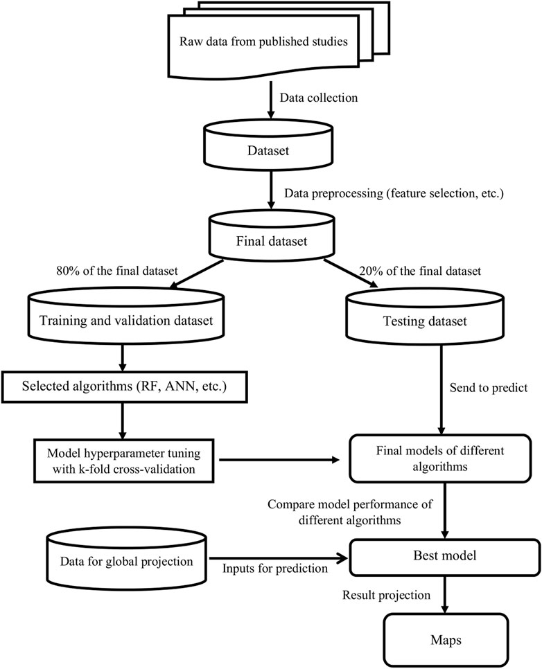
FIGURE 1. Proposed machine learning pipeline for predicting the performance of cropping systems and comparing different algorithms.

Moreover, we also developed a new evaluation metric for quantile regression, error score (ES), which can assess the overall model performance for the interval prediction ability for all quantiles, rather than simply using the traditional prediction interval coverage probability (PICP) that can only evaluate the interval prediction ability for a specific prediction interval ($1-\alpha$).

Methods

Dataset Establishment

The literature search was conducted in February 2020 using the keywords ‘conservation agriculture or no-till or no tillage or zero tillage and ‘yield or yield change’ in the websites ‘ScienceDirect’ and ‘Science Citation Index’. The details of the paper screening and data collection procedure (Supplementary Figure S1) were described in previous publications (Su et al., 2021a; Su et al., 2021b). The final dataset includes 4,403 paired yield observations for no tillage (NT) and CT under different farming practices for eight major crop species, which were extracted from 413 papers (published between 1983 and 2020). The experimental sites cover 50 countries from 1980 to 2017. This dataset contains both numerical data (such as climatic conditions, year of NT implementation) and categorical data (such as soil characteristics, crop species and different farming practices).

Model Training

A first series of models are trained to classify yield gain $\left(\frac{Yiel{d}_{CA or NT}}{Yiel{d}_{CT}}>1\right)$ versus yield loss $\left(\frac{Yiel{d}_{CA or NT}}{Yiel{d}_{CT}}<1\right)$, namely random forest (Ho, 1995) (RF), random forest with spatial correlations (Rousset and Ferdy, 2014) (RF with spaMM), gradient boosting (Friedman, 1999; Friedman, 2001) (GBM), extreme gradient boosting (Friedman, 1999; Friedman, 2001; Schmidhuber et al., 2018) (XGBOOST), artificial neural networks with different number of hidden layers (Haykin, 1998; Bergmeir and Benítez, 2012) (ANNs), k-nearest neighbours (Hastie et al., 2009) (KNN), support vector machines (Cortes and Vapnik, 1995) (SVM), naïve bayes (Hand and Yu, 2001; Hastie et al., 2009) (NB), and generalized linear model (Nelder and Wedderburn, 1972) (GLM). A second series of models are trained for quantitatively predicting the ratio of relative yield change $\frac{Yiel{d}_{CA}-Yiel{d}_{CT}}{Yiel{d}_{CT}}$, namely RF, RF with spaMM, GBM, XGBOOST, ANNs, KNN, SVM, and GLM. Finally, a third series of models are trained to predict quantiles of this relative yield change, namely quantile regression forest (Meinshausen, 2006) (QRF), quantile regression gradient boosting (Friedman, 1999; Friedman, 2001) (QRGBM), quantile regression neural networks (Cannon, 2011; Cannon, 2018) (QRNN). Thus, these models predict the ranges of relative yield change for different probability coverages.

As shown in Figure 1, all the models are trained based on 80% of the dataset, while the rest 20% is used for model testing. And these models are trained based on the model inputs that describing climate conditions over crop growing seasons (precipitation balance, minimum temperature, average temperature, and maximum temperature), soil texture, agricultural management practices (crop rotation, soil cover, fertilization, weed and pest control, irrigation and CA/NT implementation year) and location (latitude and longitude). Note that CA is defined as NT with soil cover and with crop rotation based on the FAO’s definition (Food and Agriculture Organization of the United Nations FAO, 2021). The brief description of algorithms and packages used were listed Supplementary Table S1.

Model Tuning With 10-Fold Cross-Validation

The hyperparameters of all the algorithms except GLM are tuned by searching the hyperparameter space (grid search (Chan and Treleaven, 2015), see Supplementary Table S2) for the best score of 10-fold cross-validation. In detail, the model performance under current setting of hyperparameters is calculated from 10-fold cross-validation. In each fold of the cross-validation, 90% of the training dataset are used to train the model, and 10% of the training dataset is used to test the model performance. This testing dataset is not overlapping in each fold and covers the whole dataset after the cross-validation. The cross-validation procedure was repeated for all the hyper-parameters within the searching grid, after which the hyperparameters that give the best performance are selected for use in model testing stage. As for GLM, the final model is selected with a stepwise algorithm (Venables and Ripley, 2002) implemented using the step function (from the ‘stats’ package, version 4.0.4 in R) run with AIC (Aho et al., 2014).

In cross-validation, the performance of classification model is assessed based on the area under the receiver operating characteristics curve (AUC) (Fernández, 2018). AUC corresponds to the probability that a classifier can rank a positive instance (yield gain in this case) higher than a negative one (yield loss). Thus, a higher AUC indicates a superior classification performance by the model (Fernández, 2018; Su et al., 2021a). The performance of quantitative predictions of relative yield change $\left(\frac{Yiel{d}_{CA}-Yiel{d}_{CT}}{Yiel{d}_{CT}}\right)$ is assessed using the root-mean-square error (RMSE), which estimates the differences between predictions and the observations. Lower RMSE values indicate a better model (Carpenter, 1960). Quantile regression models were assessed by comparing the coverage probability (PICP) of the range of values defined by the quantiles from $\frac{\alpha }{2}$ and $\left(1-\frac{\alpha }{2}\right)$ to its nominal target prediction interval ($1-\alpha$) (Newcombe, 1998; Landon and Singpurwalla, 2008; Wang, 2008; Khosravi et al., 2010). Here we set $(1-\alpha )=0.8$, thus, the model with the PICP value closest to 0.8 is selected as the final model (see Supplementary Figure S2).

The performances from cross-validation for all the models are presented in Supplementary Table S3–5.

Model Testing

The performances of the trained models are determined using an independent testing dataset including 20% of the total number of data (Figure 1) using the criteria AUC (Fernández, 2018) and RMSE (Carpenter, 1960) for classification models and regression models, respectively. For quantile regression models, the prediction interval coverage probability (PICP) can only represent the interval prediction ability of the model at the range defined by the quantiles from $\frac{\alpha }{2}$ and $\left(1-\frac{\alpha }{2}\right)$ (Newcombe, 1998; Landon and Singpurwalla, 2008; Wang, 2008; Khosravi et al., 2010). To assess the overall performance for all quantiles, we generalized this approach by plotting PICP vs. its corresponding prediction interval $(1-\alpha )$ for $(1-\alpha )$ ranging between 0 and 1, then comparing the resulting curve to the reference line (1:1 line). The error score (ES) is then defined by Eq. 1 and can be written as the area between the curve of PICPs vs. $(1-\alpha )$ and the 1:1 line, divided by 0.5, which serves here as a benchmark. This value of 0.5 is reached when the PICP is independent from $\alpha$. The criterion ES measures the overall performance of the model over all quantiles. Smaller ES values indicate better model interval prediction ability.

$Error Score=\frac{Area between the curve of PICPs vs. (1-\propto ) and 1:1 line }{0.5 } \times 100\%(1)$

Interval scores (IS) (Gneiting and Raftery, 2007; Papacharalampous et al., 2019) for $\left(1-\alpha \right)$ = 0.5, 0.8 and 0.9 were also calculated for different quantile regression models to cross-check the relevance of this new criterion (Supplementary Figure S3). The interval score is defined by Eq. 2, where the upper ($u$) and lower ($l$) endpoints are the predicted quantiles at levels $\frac{\alpha }{2}$ and $\left(1-\frac{\alpha }{2}\right)$, respectively. The first term of the IS indicates the range of prediction interval, while the second and third terms are the penalty scores added to this range when the observations are outside the prediction interval. For a given $\left(1-\alpha \right)$, a smaller IS indicates a better model performance.

$Interval Score=\left(u-l\right)+\frac{2}{\alpha }\left(l-x\right)1\left\{x<l\right\}+\frac{2}{\alpha }\left(x-u\right)1\{x>u\} (2)$

The final performances from model testing for all the models are presented in Supplementary Table S3–5.

Global Projection

The algorithms with the best final model performance are used for classification (yield gain vs. loss), for quantitative prediction (ratio of relative yield change of CA vs. CT), and for computing intervals (intervals of relative yield change ratios). Model outputs include the probabilities of yield gain with CA for the classification models, the relative yield change with CA for regression models, and the 10th and 90th percentiles of relative yield change for the range regression models. These outputs are mapped at the global scale with climate data over the 1981–2010 time slice at a spatial resolution of $0.5°\text{ latitude }\times 0.5°\text{ longitude}$ (average air temperature (NOAA/OAR/ESRLPSL, 2020), maximum air temperature (NOAA/OAR/ESRLPSD, 2020), minimum air temperature (NOAA/OAR/ESRLPSD, 2020), precipitation (NOAA/OAR/ESRLPSL, 2020), potential evapotranspiration (Miralles et al., 2011; Martens et al., 2017)). As for the farming practices, we set up CA as a combination of no tillage with crop rotation and with soil cover, and CT as a combination of tillage without crop rotation and without soil cover. Both systems are incorporated with fertilizer utilization and weed and pest control. All maps are generated with MATLAB R2020a (Version 9.8.0.1451342). Details of model settings for global projection and the sources of climate data and soil data are listed in Supplementary Table S6.

Results

Random forest (RF), GBM, and XGBOOST show better classification performance, with AUC values equal to 0.790, 0.786, 0.783, respectively, while the more traditional algorithms GLM and NB have lower performance, with AUC values of 0.644 and 0.647, respectively (Figure 2, Supplementary Table S3). With ANN, the best classification accuracy was obtained using two hidden layers, with an AUC value of 0.752 (Figure 2, Supplementary Table S3).

FIGURE 2

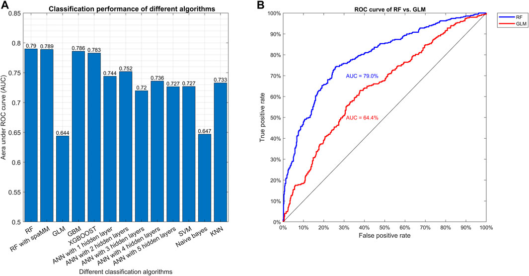
FIGURE 2. Comparison of different classification algorithms based on AUC. Plot (A) shows the AUC in the final testing step for the various algorithms after model tuning. Plot (B) shows the ROC curve of the best (RF) and the worst (GLM) algorithms.

The regression models achieved RMSEs larger than 0.25, and R squared ($R^2$) of all algorithms under 0.6 (Figure 3A, Supplementary Table S4), revealing low to moderate explanatory power. Among these algorithms, the best performance is achieved by RF, with a $R^2$ of 0.52, and a RMSE of 0.25, while GLM has the worst performance, with a $R^2$ of 0.12, and a RMSE of 0.34 (Figure 3A, Supplementary Table S4). Figures 3B,C show the scatterplot of observations versus predictions of relative crop yield change from the RF and GLM models, respectively. Predictions with GLM are poorly related to observations, while RF is able to explain a substantial fraction of the total variability.

FIGURE 3

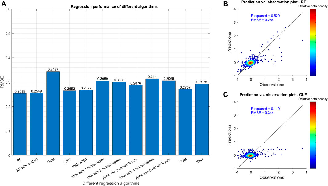
FIGURE 3. Comparison of different regression algorithms based on RMSE. Plot (A) shows the RMSE in the final testing step for the various algorithms after model tuning. The number after ANN indicates the number of hidden layers in the neural networks. Plots (B,C) are the scatterplots of observations and predictions of relative crop yield change from the best (RF) and the worst (GLM) algorithms, respectively. All the models were trained with the training dataset in which the outliers (data points outside the 95% confidence interval) were filtered.

For range regression models, different rankings are obtained depending on whether outliers in the dataset were included or not (Figure 4). With outliers included, the best performance is obtained with QRF (ES = 1.73%), while QRGBM performs better when the outliers were filtered (ES = 1.38%). QRNN performs better with one than with two hidden layers, but never outperforms QRF and QRGBM (with ES equals to 5.35 and 15.69% without and with outliers, respectively). The results of interval scores for different prediction intervals (0.5, 0.8 and 0.9) also show that QRF has the best performance among all algorithms (Supplementary Figure S3). QRGBM has a relatively low ES (Figure 4) and a relatively high IS (Supplementary Figure S3A) when the outliers are included. This indicates that, for QRGBM, the observations fall within the prediction interval in expected proportions (i.e., 0.5, 0.8 and 0.9), although relatively large errors can occur for data falling outside the prediction interval.

FIGURE 4

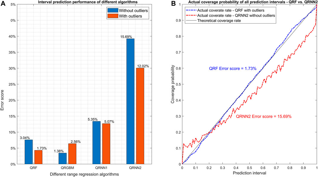
FIGURE 4. Comparison of different range regression algorithms based on ES. Plot (A) shows the error score in the final testing step for the various algorithms after model tuning. Plots (B) and c show the actual coverage rates for all the prediction intervals of the best (QRF) and worst algorithm (QRNN2). The number after QRNN indicates the number of hidden layers in the quantile regression neural networks. All the models were trained both with and without the outliers (outside 95% confidence interval) in the original dataset filtered to check if the algorithms can handle outliers.

The productivity of CA vs. CT systems for spring barley was mapped at the global scale. To reveal the differences among models, we mapped the probability of yield gain (Figures 5A,B) and relative yield change (Supplementary Figure S4) of CA vs. CT based on the results obtained with the best (RF) and the worst (GLM) algorithms. Results obtained with both algorithms show that - with fertilizer inputs and an appropriate control of weeds and pests - the probability of yield gain with CA vs. CT is higher than 0.5 in western North America, central Asia, and many regions in the east and central Africa, while the probability is lower in eastern North America and Europe (Figure 5A, Figure 5B). However, there are many inconsistencies in the predictions of the two algorithms in other regions. For example, according to RF, the use of CA instead of CT would most likely lead to yield loss (with a probability of yield gain under 0.5) in south America, and in most regions within eastern and southern Asia, while opposite results are provided by GLM in those regions (Figure 5A, Figure 5B, respectively). This contradiction reveals that the choice of an inappropriate model (such as GLM, here) would lead to wrong conclusions, highlighting the importance of the model selection step in our procedure. This is confirmed by the relative yield changes of CA vs. CT mapped with the RF and GLM models in Supplementary Figure S4. According to RF, yield gains are expected when shifting from CT to CA in western North America, central Asia, and many regions in the east and central Africa, while yield losses are predicted over most of Europe (Supplementary Figure S4A). This is in line with the results from RF classification model (Figure 5A). Conversely, according to the results of the GLM regression model, yield gains are predicted in eastern North America and Europe, while yield losses are predicted in central Asia (Supplementary Figure S4B), which is not consistent with the GLM classification model (Figure 5B) and RF models (Figure 5A, Supplementary Figure S4A).

FIGURE 5

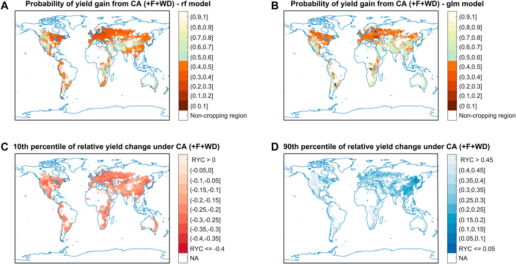
FIGURE 5. Global projection obtained with the algorithms of classification and quantile regression. Plots (A,B) show the maps of probability of barley yield gain with CA vs. CT based on the best classification (RF) and the worst (GLM) algorithms, respectively. Regions with a probability of yield gain lower than 0.5 are highlighted in red. Plots (C,D) show the maps of relative yield change with CA vs. CT under 10th and 90th percentiles, respectively, based on QRF algorithm. There was a 90% chance that the relative yield change will be higher than the ratio shown on the map in plot c, and conversely a 10% chance that the relative change will be lower.

To describe the uncertainty associated with this projection, we plotted the relative yield change of CA vs. CT that corresponding to 10th and 90th percentiles (Figures 5C,D). We show that there is 10% chance that the relative yield change of CA vs. CT will be higher than 0.45 in western North America, southern South America, eastern and central Africa (Figure 5D), while there is 10% chance that relative yield changes be lower than 0.35 in part of western North America, central Asia, and northern China (Figure 5C). We also plotted the differences between the 10th and 90th percentiles, and the results show that the uncertainty in western North America, central Africa, central Asia are relatively larger than other regions (Supplementary Figure S5).

SHAP dependence plot (Roth, 1988) was generated with respect to two control variables: the precipitation balance (PB = precipitation - evapotranspiration) (Steward et al., 2018; Su et al., 2021a; Su et al., 2021b; Su et al., 2021c) and the number of years since the switch to no tillage (NTyear). This is an alternative to partial dependence plots (PDP), and a means to assess how PB and NTyear would affect the performance of CA. While PDPs show average effects, the SHAP dependence plot also shows the variance on its y-axis. The results show that a relatively lower PB or a longer period of no tillage implementation is likely to improve the performance of CA compared to CT (Supplementary Figures S6, S7, respectively).

Discussion

In this study, we trained a broad set of machine learning (ML) models for different purposes: classification, quantitative prediction, and range prediction. This is the first time that 12 ML algorithms are implemented and compared in an application dealing with a major, global issue for agriculture. And we developed a new evaluation metric for quantile regression, the error score, based on the traditional coverage probability of a specific prediction interval, which enables us to assess the overall interval prediction ability for all quantiles and the interval prediction ability is for each prediction interval. It is a more accurate and comprehensive evaluation metric than coverage probability in evaluating and comparing quantile regression models.

Here we produced global maps obtained with the most accurate algorithms, which reveal a strong geographical variation (Sun et al., 2020; Su et al., 2021a; Su et al., 2021c) of the probability of yield gain with CA, and of the predicted relative yield change resulting from its adoption over convention tillage. This result shows that the mere presentation of an average effect size - as often done in standard meta-analyses - does not provide sufficient information on the performance of one cropping system compared to another. Contrary to standard meta-analyses, our approach can be used to describe the variability of this relative performance and to identify geographical areas where one cropping system outranks the other with a higher spatial resolution. This is an important advantage in a context where the choice of cropping systems should be adapted to the local context to provide optimal performance. Here, the global maps generated from our machine learning approach reveal that CA can be competitive in western North America and central Asia, in particular in dry regions, where CA tends to have better performance (Supplementary Figure S6). The result is consistent with recent studies (Pittelkow et al., 2015a; Pittelkow et al., 2015b; Su et al., 2021a), and related to the fact that no tillage and soil cover can reduce soil evapotranspiration (O’Leary and Connor, 1997; Nielsen et al., 2005; Page et al., 2020) and increase the water holding ability (Liu, 2013), which help the crops coping with agricultural drought, thus, potentially increasing the crop yield and CA competitiveness in dry regions.

Our comparative analysis shows that, RF has the best performance for both classification and quantitative prediction, followed by GBM, XGBOOST, ANNs, SVM, and KNN, while GLM and NB have the worst performance compared to other algorithms. The reason why RF and GBM perform better is likely linked to the type of data used for model training. As many agricultural datasets, our dataset includes both quantitative and categorical features. RF, GBM, SVM are able to handle such heterogeneous features, while ANNs, KNN, XGBOOST work usually better with numerical and homogeneous inputs (Ali et al., 2019; Zhou, 2021). Converting categorical features to numerical will also increase the number of feature inputs, it will dramatically increase the computational time for, e.g., ANNs (Nataraja and Ramesh, 2019). Moreover, the numerical features in our dataset are in very different scales, it is necessary to normalize them for ANNs and KNN to reduce effects of disparate ranges (Sarle et al., 1991; Han et al., 2011; Ali et al., 2019). Concerning SVM, it gives poor performance with large dataset (Nataraja and Ramesh, 2019). Finally, VB and GLM are often inaccurate when the data are heterogeneous and when the responses are non-linear (Nataraja and Ramesh, 2019). Other studies from agriculture-related sectors also reported similar trend in the performance of machine learning algorithms. For example, Cao et al. (2021) reported that RF had better performance than ANNs in wheat yield prediction. Rahmati et al. (2020) revealed that RF had better classification ability than SVM when predicting agricultural droughts in Australia. Dubois et al. (2021) reported that RF and SVM had better quantitative prediction ability than ANNs for forecasting soil moisture in the short-term. In other fields, Uddin et al. (2019) unveiled that in disease detection, RF had the highest chance to show excellent classification capability (with an AUC over 0.8), followed by SVM, NB, ANNs, KNN. However, RF is not systematically ranked first in previous studies (Bozdağ et al., 2020; Schwalbert et al., 2020; Khanam and Foo, 2021) and the performance of different algorithms may shift depending on the type of applications and data provided. It is therefore essential to evaluate a range of different candidate algorithms for each application, and not to systematically rely on the same approach. Our methodological framework appears very useful in this context because it allows the comparison of several algorithms on an objective basis.

Concerning interval prediction, it is reported that the performances of quantile regression algorithms often vary depending on the quantiles considered (Newcombe, 1998; Wang, 2008; David et al., 2018; He et al., 2020; Córdoba et al., 2021). This highlights the importance of evaluating these algorithms for a wide range of quantiles. In this perspective, the new evaluation metric we developed for quantile regression - error score (ES) - is meaningful and can be used to assess any quantile regression model over the whole range of quantiles. This criterion can be used to select or tune algorithms performing over a large range of quantiles and not only for specific quantile values.

In this study, we prove that the experimental data collected from published studies can be used to conduct more complex analyses via machine learning techniques (such as the random forest algorithm) than those done in standard meta-analyses, usually based on linear models. The maps created from the machine learning pipeline we proposed here provides detailed geographical information about the performance of one agricultural system compared to a reference baseline, and this pipeline can be easily adapted to analyse a diversity of outcomes or land management systems. These may involve the effects of crop management practices on soil organic carbon dynamics, greenhouse gas emissions, biodiversity, etc. for different types of cropping systems, such as organic agriculture or agroforestry, and thus provide valuable information on the local performance of sustainable farming practices together with a global perspective.

Code Availability Statement

All the R and MATLAB codes are available under request from the corresponding author.

Data Availability Statement

The datasets presented in this study can be found in online repositories. The names of the repository/repositories and accession number(s) can be found below: https://doi.org/10.6084/m9.figshare.12155553.

Author Contributions

YS wrote the main manuscript text, HZ, BG and DM modified it; YS collected the data; All authors designed the machine learning pipeline together; YS and HZ worked on the model training, model cross-validation, model testing, and model comparison; YS, BG and DM worked together to prepare the figures and tables; All authors reviewed the manuscripts.

Funding

This work was supported by the ANR under the “Investissements d’avenir” program with the reference ANR-16-CONV-0003 (CLAND) and by the INRAE CIRAD meta-program “GloFoods”.

Conflict of Interest

The authors declare that the research was conducted in the absence of any commercial or financial relationships that could be construed as a potential conflict of interest.

Publisher’s Note

All claims expressed in this article are solely those of the authors and do not necessarily represent those of their affiliated organizations, or those of the publisher, the editors and the reviewers. Any product that may be evaluated in this article, or claim that may be made by its manufacturer, is not guaranteed or endorsed by the publisher.

Supplementary Material

The Supplementary Material for this article can be found online at: https://www.frontiersin.org/articles/10.3389/fenvs.2022.812648/full#supplementary-material

References

Aho, K., Derryberry, D., and Peterson, T. (2014). Model Selection for Ecologists: the Worldviews of AIC and BIC. Ecology 95, 631–636. doi:10.1890/13-1452.1

PubMed Abstract | CrossRef Full Text | Google Scholar

Ali, N., Neagu, D., and Trundle, P. (2019). Classification of Heterogeneous Data Based on Data Type Impact on Similarity. Editors. A. Lotfi, H. Bouchachia, A. Gegov, C. Langensiepen, and M. McGinnity (Springer International Publishing). doi:10.1007/978-3-319-97982-3_21

CrossRef Full Text | Google Scholar

Bergmeir, C., and Benítez, J. M. (2012). Neural Networks in R Using the Stuttgart Neural Network Simulator: RSNNS. J. Stat. Softw. 46. doi:10.18637/jss.v046.i07

CrossRef Full Text | Google Scholar

Bozdağ, A., Dokuz, Y., and Gökçek, Ö. B. (2020). Spatial Prediction of PM10 Concentration Using Machine Learning Algorithms in Ankara, Turkey. Environ. Pollut. 263, 114635. doi:10.1016/j.envpol.2020.114635

PubMed Abstract | CrossRef Full Text | Google Scholar

Cannon, A. J. (2018). Non-crossing Nonlinear Regression Quantiles by Monotone Composite Quantile Regression Neural Network, with Application to Rainfall Extremes. Stoch Environ. Res. Risk Assess. 32, 3207–3225. doi:10.1007/s00477-018-1573-6

CrossRef Full Text | Google Scholar

Cannon, A. J. (2011). Quantile Regression Neural Networks: Implementation in R and Application to Precipitation Downscaling. Comput. Geosciences 37, 1277–1284. doi:10.1016/j.cageo.2010.07.005

CrossRef Full Text | Google Scholar

Cao, J., Zhang, Z., Luo, Y., Zhang, L., Zhang, J., Li, Z., et al. (2021). Wheat Yield Predictions at a County and Field Scale with Deep Learning, Machine Learning, and Google Earth Engine. Eur. J. Agron. 123, 126204. doi:10.1016/j.eja.2020.126204

CrossRef Full Text | Google Scholar

Carpenter, R. G. (1960). Principles and Procedures of Statistics, with Special Reference to the Biological Sciences. Eugenics Rev. 52, 172–173.

Google Scholar

Chan, S., and Treleaven, P. (2015). Continuous Model Selection for Large-Scale Recommender Systems. doi:10.1016/b978-0-444-63492-4.00005-8

CrossRef Full Text | Google Scholar

Corbeels, M., Naudin, K., Whitbread, A. M., Kühne, R., and Letourmy, P. (2020). Limits of Conservation Agriculture to Overcome Low Crop Yields in Sub-saharan Africa. Nat. Food 1, 447–454. doi:10.1038/s43016-020-0114-x

CrossRef Full Text | Google Scholar

Córdoba, M., Carranza, J. P., Piumetto, M., Monzani, F., and Balzarini, M. (2021). A Spatially Based Quantile Regression forest Model for Mapping Rural Land Values. J. Environ. Manage. 289, 112509. doi:10.1016/j.jenvman.2021.112509

CrossRef Full Text | Google Scholar

Cortes, C., and Vapnik, V. (1995). Support-vector Networks. Mach Learn. 20, 273–297. doi:10.1007/bf00994018

CrossRef Full Text | Google Scholar

David, M., Luis, M. A., and Lauret, P. (2018). Comparison of Intraday Probabilistic Forecasting of Solar Irradiance Using Only Endogenous Data. Int. J. Forecast. 34, 529–547. doi:10.1016/j.ijforecast.2018.02.003

CrossRef Full Text | Google Scholar

Dubois, A., Teytaud, F., and Verel, S. (2021). Short Term Soil Moisture Forecasts for Potato Crop Farming: A Machine Learning Approach. Comput. Electro. Agric. 180, 105902. doi:10.1016/j.compag.2020.105902

CrossRef Full Text | Google Scholar

Eisler, I. (1990). Meta-analysis: Magic wand or exploratory tool? Comment on Markus et al. J. Fam. Ther. 12, 223–228. doi:10.1046/j.1990.00389.x

CrossRef Full Text | Google Scholar

Farooq, M., and Siddique, K. H. M. (2015). Conservation Agriculture. Springer.

Google Scholar

Fernández, A. (2018). Learning from Imbalanced Data Sets. Springer International Publishing.

Google Scholar

Fitz-Gibbon, C. T. (1984). Meta-Analysis: An Explication. Br. Educ. Res. J. 10, 135–144.

Google Scholar

Flather, M. D., Farkouh, M. E., Pogue, J. M., and Yusuf, S. (1997). Strengths and Limitations of Meta-Analysis: Larger Studies May Be More Reliable. Controlled Clin. Trials 18, 568–579. doi:10.1016/s0197-2456(97)00024-x

PubMed Abstract | CrossRef Full Text | Google Scholar

Food and Agriculture Organization of the United Nations FAO (2021). Conservation Agriculture. Available at: http://www.fao.org/conservation-agriculture/en/ (Accessed May 16, 2021).

Google Scholar

Friedman, J. H. (2001). Greedy Function Approximation: A Gradient Boosting Machine. Ann. Stat. 29. doi:10.1214/aos/1013203451

CrossRef Full Text | Google Scholar

Friedman, J. H. (1999). Stochastic Gradient Boosting. Comput. Stat. Data Anal. 38, 367–378.

Google Scholar

Gneiting, T., and Raftery, A. E. (2007). Strictly Proper Scoring Rules, Prediction, and Estimation. J. Am. Stat. Assoc. 102, 359–378. doi:10.1198/016214506000001437

CrossRef Full Text | Google Scholar

González-Chávez, M. d. C. A., Aitkenhead-Peterson, J. A., Gentry, T. J., Zuberer, D., Hons, F., and Loeppert, R. (2010). Soil Microbial Community, C, N, and P Responses to Long-Term Tillage and Crop Rotation. Soil Tillage Res. 106, 285–293. doi:10.1016/j.still.2009.11.008

CrossRef Full Text | Google Scholar

Goulding, K. W. T., Trewavas, A., and Giller, K. E. (2011). Feeding the World: a Contribution to the Debate. World Agric. 2, 32–38.

Google Scholar

Govaerts, B., Fuentes, M., Mezzalama, M., Nicol, J. M., Deckers, J., Etchevers, J. D., et al. (2007). Infiltration, Soil Moisture, Root Rot and Nematode Populations after 12 Years of Different Tillage, Residue and Crop Rotation Managements. Soil Tillage Res. 94, 209–219. doi:10.1016/j.still.2006.07.013

CrossRef Full Text | Google Scholar

Han, J., Pei, J., and Kamber, M. (2011). Data Mining: Concepts and Techniques. Elsevier.

Google Scholar

Hand, D. J., and Yu, K. (2001). Idiot's Bayes: Not So Stupid after All. Int. Stat. Rev./Revue Internationale de Statistique 69, 385. doi:10.2307/1403452

CrossRef Full Text | Google Scholar

Hastie, T., Tibshirani, R., and Friedman, J. (2009). The Elements of Statistical Learning. New York: Springer.

Google Scholar

Haykin, S. (1998). Neural Networks: A Comprehensive Foundation. New Jersey: Prentice Hall PTR.

Google Scholar

He, F., Zhou, J., Mo, L., Feng, K., Liu, G., and He, Z. (2020). Day-ahead Short-Term Load Probability Density Forecasting Method with a Decomposition-Based Quantile Regression forest. Appl. Energ. 262, 114396. doi:10.1016/j.apenergy.2019.114396

CrossRef Full Text | Google Scholar

Ho, T. K. (1995). “Random Decision Forests,” in Proceedings of 3rd International Conference on Document Analysis and Recognition.

Google Scholar

Holland, J. M. (2004). The Environmental Consequences of Adopting Conservation Tillage in Europe: Reviewing the Evidence. Agric. Ecosyst. Environ. 103, 1–25. doi:10.1016/j.agee.2003.12.018

CrossRef Full Text | Google Scholar

Kassam, A., Friedrich, T., Shaxson, F., and Pretty, J. (2009). The Spread of Conservation Agriculture: Justification, Sustainability and Uptake. Int. J. Agric. Sustainability 7, 292–320. doi:10.3763/ijas.2009.0477

CrossRef Full Text | Google Scholar

Khanam, J. J., and Foo, S. Y. (2021). A Comparison of Machine Learning Algorithms for Diabetes Prediction. ICT Express 7, 432–439. doi:10.1016/j.icte.2021.02.004

CrossRef Full Text | Google Scholar

Khosravi, A., Nahavandi, S., and Creighton, D. (2010). Construction of Optimal Prediction Intervals for Load Forecasting Problems. IEEE Trans. Power Syst. 25, 1496–1503. doi:10.1109/tpwrs.2010.2042309

CrossRef Full Text | Google Scholar

Krupnik, T. J., Andersson, J. A., Rusinamhodzi, L., Corbeels, M., Shennan, C., and Gérard, B. (2019). Does Size Matter? A Critical Review of Meta-Analysis in Agronomy. Ex. Agric. 55, 200–229. doi:10.1017/s0014479719000012

CrossRef Full Text | Google Scholar

Landon, J., and Singpurwalla, N. D. (2008). Choosing a Coverage Probability for Prediction Intervals. The Am. Statistician 62, 120–124. doi:10.1198/000313008x304062

CrossRef Full Text | Google Scholar

Liu, Y. (2013). Effects of Conservation Tillage Practices on the Soil Water-Holding Capacity of a Non-irrigated Apple Orchard in the Loess Plateau. China, 130 7–12.

Google Scholar

Martens, B., Miralles, D. G., Lievens, H., van der Schalie, R., de Jeu, R. A. M., Fernández-Prieto, D., et al. (2017). GLEAM V3: Satellite-Based Land Evaporation and Root-Zone Soil Moisture. Geosci. Model. Dev. 10, 1903–1925. doi:10.5194/gmd-10-1903-2017

CrossRef Full Text | Google Scholar

Meinshausen, N. (2006). Quantile Regression Forests. J. Machine Learn. Res. 7, 983–999.

Google Scholar

Michler, J. D., Baylis, K., Arends-Kuenning, M., and Mazvimavi, K. (2019). Conservation Agriculture and Climate Resilience. J. Environ. Econ. Manag. 93, 148–169. doi:10.1016/j.jeem.2018.11.008

CrossRef Full Text | Google Scholar

Miralles, D. G., Holmes, T. R. H., De Jeu, R. A. M., Gash, J. H., Meesters, A. G. C. A., and Dolman, A. J. (2011). Global Land-Surface Evaporation Estimated from Satellite-Based Observations. Hydrol. Earth Syst. Sci. 15, 453–469. doi:10.5194/hess-15-453-2011

CrossRef Full Text | Google Scholar

Nataraja, P., and Ramesh, B. (2019). Machine Learning Algorithms for Heterogeneous Data: A Comparative Study. Int. J. Comp. Eng. Tech. 10. doi:10.34218/ijcet.10.3.2019.002

CrossRef Full Text | Google Scholar

Nelder, J. A., and Wedderburn, R. W. M. (1972). Generalized Linear Models. J. R. Stat. Soc. Ser. A (General) 135, 370. doi:10.2307/2344614

CrossRef Full Text | Google Scholar

Newcombe, R. G. (1998). Two-sided Confidence Intervals for the Single Proportion: Comparison of Seven Methods. Statist. Med. 17, 857–872. doi:10.1002/(sici)1097-0258(19980430)17:8<857:aid-sim777>3.0.co;2-e

CrossRef Full Text | Google Scholar

Nielsen, D. C., Unger, P. W., and Miller, P. R. (2005). Efficient Water Use in Dryland Cropping Systems in the Great Plains. Agron.j. 97, 364–372. doi:10.2134/agronj2005.0364

CrossRef Full Text | Google Scholar

NOAA/OAR/ESRL PSD, (2020). CPC Global Daily Temperature. Available at: https://www.esrl.noaa.gov/psd/data/gridded/data.cpc.globaltemp.html (Accessed February 25, 2020).

Google Scholar

NOAA/OAR/ESRL PSL, (2020). University of Delaware Air Temperature & Precipitation. Available at: https://www.esrl.noaa.gov/psd/data/gridded/data.UDel_AirT_Precip.html (Accessed February 25, 2020).

Google Scholar

O’Leary, G. J., and Connor, D. J. (1997). Stubble Retention and Tillage in a Semi-arid Environment: 1. Soil Water Accumulation during Fallow. Field Crops Res. 52, 209–219.

Google Scholar

Ortiz-Bobea, A., Ault, T. R., Carrillo, C. M., Chambers, R. G., and Lobell, D. B. (2021). Anthropogenic Climate Change Has Slowed Global Agricultural Productivity Growth. Nat. Clim. Chang. 11, 306–312. doi:10.1038/s41558-021-01000-1

CrossRef Full Text | Google Scholar

Page, K. L., Dang, Y. P., and Dalal, R. C. (2020). The Ability of Conservation Agriculture to Conserve Soil Organic Carbon and the Subsequent Impact on Soil Physical, Chemical, and Biological Properties and Yield. Front. Sustain. Food Syst. 4. doi:10.3389/fsufs.2020.00031

CrossRef Full Text | Google Scholar

Papacharalampous, G., Tyralis, H., Langousis, A., Jayawardena, A. W., Sivakumar, B., Mamassis, N., et al. (2019). Probabilistic Hydrological Post-Processing at Scale: Why and How to Apply Machine-Learning Quantile Regression Algorithms. Water 11, 2126. doi:10.3390/w11102126

CrossRef Full Text | Google Scholar

Pittelkow, C. M., Liang, X., Linquist, B. A., van Groenigen, K. J., Lee, J., Lundy, M. E., et al. (2015b). Productivity Limits and Potentials of the Principles of Conservation Agriculture. Nature 517, 365–368. doi:10.1038/nature13809

PubMed Abstract | CrossRef Full Text | Google Scholar

Pittelkow, C. M., Linquist, B. A., Lundy, M. E., Liang, X., van Groenigen, K. J., Lee, J., et al. (2015a). When Does No-Till Yield More? A Global Meta-Analysis. Field Crops Res. 183, 156–168. doi:10.1016/j.fcr.2015.07.020

CrossRef Full Text | Google Scholar

Pradhan, A., Chan, C., Roul, P. K., Halbrendt, J., and Sipes, B. (2018). Potential of Conservation Agriculture (CA) for Climate Change Adaptation and Food Security under Rainfed Uplands of India: A Transdisciplinary Approach. Agric. Syst. 163, 27–35. doi:10.1016/j.agsy.2017.01.002

CrossRef Full Text | Google Scholar

Rahmati, O., Falah, F., Dayal, K. S., Deo, R. C., Mohammadi, F., Biggs, T., et al. (2020). Machine Learning Approaches for Spatial Modeling of Agricultural Droughts in the South-East Region of Queensland Australia. Sci. Total Environ. 699, 134230. doi:10.1016/j.scitotenv.2019.134230

PubMed Abstract | CrossRef Full Text | Google Scholar

Renard, D., and Tilman, D. (2019). National Food Production Stabilized by Crop Diversity. Nature 571, 257–260. doi:10.1038/s41586-019-1316-y

PubMed Abstract | CrossRef Full Text | Google Scholar

Roth, A. E. (1988). The Shapley Value. Cambridge, United Kingdom: Cambridge University Press. doi:10.1017/CBO9780511528446

CrossRef Full Text | Google Scholar

Rousset, F., and Ferdy, J.-B. (2014). Testing Environmental and Genetic Effects in the Presence of Spatial Autocorrelation. Ecography 37, 781–790. doi:10.1111/ecog.00566

CrossRef Full Text | Google Scholar

Sarle, W. S., Kaufman, L., and Rousseeuw, P. J. (1991). Finding Groups in Data: An Introduction to Cluster Analysis. J. Am. Stat. Assoc. 86, 830. doi:10.2307/2290430

CrossRef Full Text | Google Scholar

Schmidhuber, J., Sur, P., Fay, K., Huntley, B., Salama, J., Lee, A., et al. (2018). The Global Nutrient Database: Availability of Macronutrients and Micronutrients in 195 Countries from 1980 to 2013. Lancet Planet. Health 2, e353–e368. doi:10.1016/s2542-5196(18)30170-0

PubMed Abstract | CrossRef Full Text | Google Scholar

Schmidt, J., Marques, M. R. G., Botti, S., and Marques, M. A. L. (2019). Recent Advances and Applications of Machine Learning in Solid-State Materials Science. Npj Comput. Mater. 5, 83. doi:10.1038/s41524-019-0221-0

CrossRef Full Text | Google Scholar

Schwalbert, R. A., Amado, T., Corassa, G., Pott, L. P., Prasad, P. V. V., and Ciampitti, I. A. (2020). Satellite-based Soybean Yield Forecast: Integrating Machine Learning and Weather Data for Improving Crop Yield Prediction in Southern Brazil. Agric. For. Meteorology 284, 107886. doi:10.1016/j.agrformet.2019.107886

CrossRef Full Text | Google Scholar

Scopel, E., Triomphe, B., Affholder, F., Da Silva, F. A. M., Corbeels, M., Xavier, J. H. V., et al. (2013). Conservation Agriculture Cropping Systems in Temperate and Tropical Conditions, Performances and Impacts. A Review. Agron. Sustain. Dev. 33, 113–130. doi:10.1007/s13593-012-0106-9

CrossRef Full Text | Google Scholar

Steward, P. R., Dougill, A. J., Thierfelder, C., Pittelkow, C. M., Stringer, L. C., Kudzala, M., et al. (2018). The Adaptive Capacity of Maize-Based Conservation Agriculture Systems to Climate Stress in Tropical and Subtropical Environments: A Meta-Regression of Yields.. Agric. Ecosyst. Environ. 251, 194–202. doi:10.1016/j.agee.2017.09.019

CrossRef Full Text | Google Scholar

Su, Y., Gabrielle, B., Beillouin, D., and Makowski, D. (2021a). High Probability of Yield Gain through Conservation Agriculture in Dry Regions for Major Staple Crops. Sci. Rep. 11, 3344. doi:10.1038/s41598-021-82375-1

PubMed Abstract | CrossRef Full Text | Google Scholar

Su, Y., Gabrielle, B., and Makowski, D. (2021b). A Global Dataset for Crop Production under Conventional Tillage and No Tillage Systems. Sci. Data 8, 33. doi:10.1038/s41597-021-00817-x

CrossRef Full Text | Google Scholar

Su, Y., Gabrielle, B., and Makowski, D. (2021c). The Impact of Climate Change on the Productivity of Conservation Agriculture. Nat. Clim. Change. doi:10.1038/s41558-021-01075-w

CrossRef Full Text | Google Scholar

Sun, W., Canadell, J. G., Yu, L., Yu, L., Zhang, W., Smith, P., et al. (2020). Climate Drives Global Soil Carbon Sequestration and Crop Yield Changes under Conservation Agriculture. Glob. Change Biol. 26, 3325–3335. doi:10.1111/gcb.15001

CrossRef Full Text | Google Scholar

Uddin, S., Khan, A., Hossain, M. E., and Moni, M. A. (2019). Comparing Different Supervised Machine Learning Algorithms for Disease Prediction. BMC Med. Inform. Decis. Mak 19, 281. doi:10.1186/s12911-019-1004-8

PubMed Abstract | CrossRef Full Text | Google Scholar

Venables, W. N., and Ripley, B. D. (2002). Modern Applied Statistics with S. New York: Springer. doi:10.1007/978-0-387-21706-2

CrossRef Full Text | Google Scholar

Walker, E., Hernandez, A. V., and Kattan, M. W. (2008). Meta-analysis: Its Strengths and Limitations. Cleveland Clinic J. Med. 75, 431–439. doi:10.3949/ccjm.75.6.431

CrossRef Full Text | Google Scholar

Wang, H. (2008). Coverage Probability of Prediction Intervals for Discrete Random Variables. Comput. Stat. Data Anal. 53, 17–26. doi:10.1016/j.csda.2008.07.017

CrossRef Full Text | Google Scholar

Zhou, Z.-H. (2021). Machine Learning. Springer Singapore.

Google Scholar