Employing the agricultural classification and estimation service (ACES) for mapping smallholder rice farms in Bhutan

1 Introduction

The unique vantage point of Earth observation (EO) data and their ability to provide ubiquitous global coverage, a diverse range of information, as well as frequent revisit rates has unlocked previously incomprehensible sources and avenues for addressing global challenges and development goals, especially pertaining to food security (Griggs et al., 2013; Assembly, 2015; Dhu et al., 2017). To that, EO based approaches have long been utilized as a key tool in crop type mapping (McNairn and Brisco, 2004; Steele-Dunne et al., 2017). Within recent years, more approaches are actively leveraging analysis ready data (ARD) and pixel based classification approaches (Orynbaikyzy et al., 2019; Tamiminia et al., 2020; Yang et al., 2022).

However, with the access and availability of geospatial and EO data rapidly increased, there has remained a gap for enabling end-users to readily apply and make decisions using EO data (Giuliani et al., 2017; Nativi et al., 2019; Gomes et al., 2020). In particular, leveraging EO to address agriculture and food security issues in geophysically complex locations, either due to terrain, cloud cover, or sparse data, remains an obstacle for the remote sensing community (Li et al., 2018; Flores-Anderson et al., 2019; Jiang et al., 2021). Additionally, developing a robust and transparent sampling approach and modeling framework to combat these two issues remains a challenge (Stehman, 2005; Olofsson et al., 2014; Bey et al., 2016).

As part of the “Advancing Science, Technology, Engineering, and Mathematics in Bhutan through Increased Earth Observation Capacity” initiative, our research team enabled 1) the use of EO into the decision making process with our Bhutan partners; 2) developed a geospatial web application and software system known as Agricultural Classification and Estimation Service (ACES) to combat the various geophysical limitations and unique challenges within Bhutan; and 3) co-developed and deployed a robust sampling and modeling framework for the country-level ACES application. This article will specifically outline the ACES geospatial application’s climate smart approach and provide a clear outline of the methodologies employed for future implementation of the framework for end-users.

2 Materials and methods

2.1 Study area and time period

The 38,394 km² Kingdom of Bhutan is predominantly a mountainous country (Gilani et al., 2015; Bureau, 2022). Bhutan is located between China and India amidst the Himalayan range, see Figure 1, and is comprised of six ecological zones: alpine, cool temperate, warm temperate, dry sub-tropical, humid-subtropical, and wet sub-tropical (Agriculture, B. M. and Forests, 1992; Bureau, 2022). The elevation range of these zones are between 100 m to over 7,500 m moving on a latitudinal gradient south to north (Ohsawa, 1987; Katwal, 2013; Bruggeman et al., 2016; Hydrology, N. C. and Meteorology, 2019). Across Bhutan, the country experiences a variety of climactic conditions due to the topography, with the following seasons: spring, summer, autumn, winter, and a Monsoon season beginning in June and ending in September (Tobgay, 2006; Chhogyel and Kumar, 2018; Hydrology, N. C. and Meteorology, 2020). A majority of the population resides in valleys and lowlands, which is primarily where agriculture cultivation is located (Walcott, 2009).

FIGURE 1

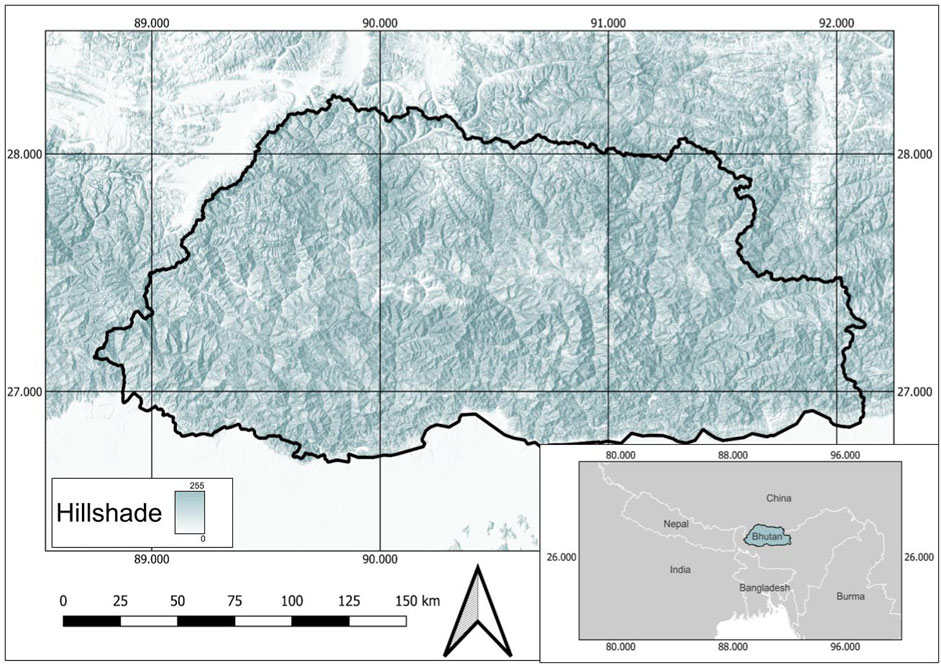
FIGURE 1. Study area map of the Kingdom of Bhutan.

Within Bhutan, rice plays a central role both culturally and as a key driver for national food security (Tshewang et al., 2016). Rice is the main food staple in the country. It is grown across the country but predominantly cultivated in three dzongkhags (districts), specifically Samtse, Punakha, and Sarpang, and national reporting is provided at the gewog (sub-district) level (Bureau, 2022). Over the past 3 decades, there has been minimal reported agricultural expansion across Bhutan, with agriculture comprising only 2.8% of the total area (Gilani et al., 2015; Uddin et al., 2021; Bureau, 2022). Additionally, the majority of agriculture within Bhutan is dominated by subsistence farming, and the average smallholder farm is 3 acres per household (Statistics, N. B, 2012; Katwal, 2013). Due to the extreme topography of Bhutan there are a range of rice cultivation strategies, the two prevalent methods are: irrigated lowland paddy fields (200–700 m above sea level) and upland terraced paddy fields (Bureau, 2021) (700–1,600 m above sea level) which account for 80% of the total national rice production (Ghimiray, 2012; Neuhoff et al., 2014). In Bhutan, there are three main phases for rice cultivation efforts consisting of nursery production, transplantation, and harvest. These align with the 5 distinct stages of rice plant develop: 1) growth of both tillers and leaves from the main stem; 2) stem development and elongation, both stages occurring in the nursery production phase; 3) defined stems as known as tillering; 4) leaf senescence, both stages in the transplantation phase; and 5) panicle and grain development concluding with the harvesting phase (Nelson et al., 2014). This is relevant as the modeling effort aims to focus on rice production fields across these phenological distinct stages through including a range of EO indices to capture phenological characteristics as well as observable cultivation practices during the key growing season of rice (May-October) (Tobgay, 2006). The focus of this research and paper was for the entire country of Bhutan, producing country wide rice classification maps for the years 2016–2021.

2.2 Existing approaches

Pertaining to crop type mapping and rice classification specifically previous studies have focused on course resolution, 500 m, wall to wall country or regional level maps (Gumma et al., 2011) or finer resolution maps at 30 m, but only for specific cultivation zones (Tashi, 2018). Building upon applications using Landsat (Dong et al., 2016), Sentinel-2 (Ni et al., 2021) and Sentinel-1 (Park et al., 2018; O’Shea et al., 2020), The ACES platform leverages an array of spatial resolutions to produce countrywide annual rice maps. This platform’s seamless combination of EO data sets allows for rapid implementation and classification at vast scales. Over the past decade, crop type mapping methods have been rapidly diversifying due to new data sources and scalable cloud technologies. These methods include phenological response mapping or temporal fitting (Xiao et al., 2006; Brown et al., 2012), leveraging derived optical and radar indices (Oguro et al., 2001; Nguyen et al., 2012; Chen et al., 2016), and algorithm approaches such as object-oriented machine learning or deep learning image analyses (Zhang et al., 2009; Lasko et al., 2018; Singha et al., 2019; Poortinga et al., 2021). These advancements in crop type mapping, specifically rice mapping and field extent mapping methods, integrate traditional knowledge of crop growth cycles with multi-source Earth observing data (Zhao et al., 2021). Through recent progress of cloud computing platforms like Google Earth Engine (GEE), remote sensing and data analysis tools are becoming increasingly centralized and more easy to facilitate multi-source data techniques, large-scale analyses, and the incorporation of auxiliary data sets for agricultural mapping purposes (Gorelick, 2013; Dong et al., 2016; Carrasco et al., 2019; Chong et al., 2021).

Due to the extreme terrain and remote nature of Bhutan, developing an EO-informed framework that centralizes field and training data collection, model generation of classified crop type, in this case rice, and incorporates climatic data was critical for enabling country-level decision making. This prompted the need to co-develop a geospatial service. The SERVIR Service Planning Toolkit was leveraged with partners at the Bhutan Department of Agriculture, the National Plant Protection Center, the National Statistics Bureau, and the Ugyen Wangchuck Institute for Conservation and Environment to co-develop the ACES web application and software package (Frankel-Reed, 2018; Searby et al., 2019; Thapa et al., 2021).

2.3 Earth observation data

2.3.1 Optical

Optical EO were obtained using the GEE platform. The ACES platform can leverage the following optical imagery: Landsat 8 Collection 2 Tier 1 calibrated top-of-atmosphere (TOA) reflectance, Landsat 8 Operational Land Imager (OLI)/Thermal Infrared Sensor (TIRS) Level 2 Collection 2, Landsat 7 Level 2, Collection 2, Tier 1 Enhanced Thematic Mapper Plus (ETM+), and Sentinel-2 (S-2) MultiSpectral Instrument (MSI) Level-2A imagery.

As part of the ARD ingestion process on the GEE platform, the Landsat 8 collection was computed to top-of-atmosphere resulting in a pre-processed Landsat 8 Collection 2 Tier 1 calibrated TOA reflectance data set (Chander et al., 2009). Additionally, the Landsat 8 collection has been pre-processed to surface reflectance using the Land Surface Reflectance Code (LaSRC) algorithm (Landsat, 2022). The Landsat 7 ETM + surface reflectance was created using the Landsat Ecosystem Disturbance Adaptive Processing System (LEDAPS) algorithm (Schmidt et al., 2013). The S-2 MSI was pre-processed using sen2cor to create the surface reflectance (Main-Knorn et al., 2017). All the aforementioned data sets are available in GEE as ARD image collections to then be utilized by ACES software system.

Landsat imagery is managed by and can be alternately accessed from the National Aeronautics and Space Administration (NASA) and the United States Geological Survey (USGS). The Landsat mission offers imagery at 30 m spatial resolution for blue, green, red, Near-Infrared (NIR), and Short-Wave Infrared 1 and 2 (SWIR 1 and 2) bands on a 16-day repeat cycle. While the European Space Agency (ESA) provides the S-2 sensor data which operates at a 10 m spatial resolution for the blue, green, red, and NIR bands, and at a 20 m resolution for the SWIR 1 and 2 bands. S-2 has the advantage of a 5–10-day repeat cycle when both of the two sensors are used. With moderate to high spatial resolutions and repeat cycles, Landsat and S-2 are suitable for crop mapping. Relying on the ACES software system, all optical image collections were further pre-processed in GEE to remove shadows and clouds using the QA pixels bands, methods and examples available in the Supporting Material section. Optical indices were then derived on the cloud free images, using the ACES system.

2.3.2 Sentinel-1

Sentinel-1 (S-1), an active Synthetic Aperture Radar (SAR) C-band sensor, was used in this framework. This sensor has the ability to collect data in distinct polarizations and operate in multiple acquisition modes at various ground sampling distances (GSD) (Mayer et al., 2021). The S-1 provides Level-1 Interferometric Wide Swath (IW) mode and Ground Range Detected (GRD) data set with a spatial resolution of 10 m (Potin et al., 2012). The S-1 GRD image collection available in GEE was ingested and pre-processed using the Sentinel-1 SNAP7 Toolbox (Sentinel Application Platform, http://step.esa.int/main/toolboxes/snap/). Wherein GRD border noise reduction, thermal noise reduction, and radiometric calibration were then performed, followed by a geometric terrain correction using the Shuttle Radar Topography Mission (STRM) to produce a standard radar backscatter data set in dB units as the final image collection available in GEE (Farr et al., 2007).

The SAR imagery was then further pre-processed using the ACES system. A Radiometric Terrain Flattening Algorithm (Small, 2011; Reiche, 2015; Vollrath et al., 2020) was applied, followed by a Lee-sigma speckle filtering (Lee et al., 2008; Huang C. et al., 2018)approach to reduce noise. The S-1 image collection was then filtered for IW Swath mode and sorted into ascending and descending Vertical-Vertical VV) and Vertical-Horizontal (VH) transmitter-receiver polarizations data sets resulting in the final pre-processed S-1 SAR image collection, all of which is done automatically using ACES. Like S-2, S-1 is provided by ESA. S-1 provides 10 m spatial resolution and a 6–10-day repeat cycle when both S-1 A and S-1 B sensors are combined.

2.3.3 Additional data sets

High-resolution imagery available through Norway’s International Climate and Forests Initiative (NICFI) provides monthly and biannual Planet imagery mosaics of the tropics. Planet and NICFI Basemaps for Tropical Forest Monitoring were used in the training data collection and independent model validation steps. The NICFI Basemaps are available at approximately 5 m spatial resolution, with new maps produced on a monthly and biannual basis (Team, 2017). The PlanetScope Dove satellite system, used for these steps, is equipped with spectral bands including Blue (455–515 nm), Green (500–590 nm), Red (590–670 nm), and NIR (780–860 nm) (Lemajic and Åstrand, 2018). This NICFI imagery was accessed via GEE. The imagery was imported into the Collect Earth Online (CEO) (Saah et al., 2019) platform for the training data collection and independent model validation efforts. Additionally, the Digital Elevation Model (DEM) 30 m data from the Shuttle Radar Topography Mission (SRTM) (Farr et al., 2007) was also used. Specifically, the elevation and derived slope were used as input features. The SRTM DEM data set is available in GEE as an existing image.

2.3.4 Indices

Band indices from optical and SAR imagery can improve the detection or quantification of specific surface characteristics. The Normalized Difference Vegetation Index (NDVI) and Soil-Adjusted Vegetation Index (SAVI) are well-established indices calculated from optical imagery used in vegetation monitoring. The number of publications using NDVI for vegetation monitoring has been increasing and has been shown to be informative for detecting focal vegetation or agriculture classes (Rouse Jr et al., 1973; Huang et al., 2021). Similarly, the SAVI is sensitive to vegetation, but adjusts for soil-vegetation interactions (Huete, 1988). The Normalized Difference Water Index (NDWI) and the Modified Normalized Difference Water Index (MNDWI) exploit the differences between reflectance in the green and the NIR and SWIR 1 bands, respectively, highlighting the presence of water or flooded fields (McFeeters, 1996; Xu, 2006). The Normalized Difference Moisture Index (NDMI) index is used to quantify vegetation water content and can also signify the presence of vegetation. Previous studies have used NDMI, often alongside SAR, to quantify soil moisture or discriminate crops for agricultural applications (Kyere et al., 2020; Tripathi and Tiwari, 2022). Additionally, tasseled caps indices, using Landsat 8 EO optical TOA imagery, produced brightness, greenness, wetness, fourth, fifth, and sixth indices which were calculated using bandwise computations, outlined in Table 1. All computations and generation of indices were performed using the ACES system in GEE (Kauth and Thomas, 1976; Crist and Kauth, 1986; Baig et al., 2014).

TABLE 1

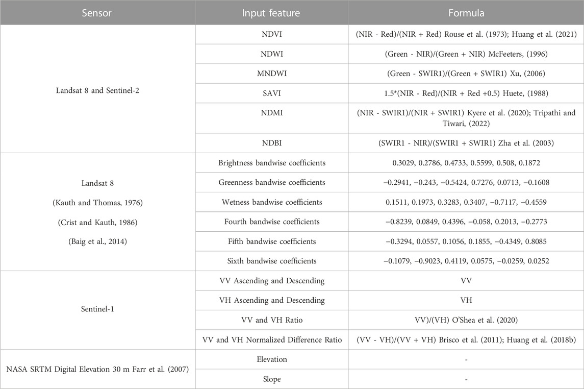
TABLE 1. Set of 28 EO derived features used for model inputs in the ACES system.

However, optical sensors like Landsat are limited by cloud cover and heavy rainfall. SAR bypasses issues of cloud cover and adds information about the structure of the land surface (Flores-Anderson et al., 2019). SAR indices not only complement optical imagery by filling in these information gaps but can also be important predictors of rice presence in studies implementing similar modeling efforts (O’Shea et al., 2020). The structure of both lowland and upland rice fields in Bhutan are generally arranged linearly within a field, where transplanted rice crops display a vertical structure during the growing season. This vertical structure exhibits volume scattering and double bounce scattering properties; these scattering types are considered relatively sensitive to VV and VH polarizations (Flores-Anderson et al., 2019). For this reason, SAR indices such as the (VV)/(VH) ratio and the normalized difference ratio have been used to effectively distinguish the unique structural signature of rice in Asia (Brisco et al., 2011; Chen et al., 2016; Lasko et al., 2018). Overall the integration of optical and SAR data has been shown to enhance the accuracy of rice mapping (Choudhury, 2004; Zhao et al., 2021).

Data was acquired according to availability within the study period and the phenology of rice. Landsat 7 was not used for the following analysis; however, the ACES platform allows end-users to leverage this sensor for future historical analyses. For Landsat 8, S-2, and S-1, a median composite for the growing season months May-October was utilized to derive the input features. Lastly, a DEM and derived elevation and slope products were used as input features. In total, 28 EO features were employed as model inputs, all of which are displayed in Table 1.

2.4 Training sample design

To effectively detect the focal class of rice using a machine learning approach, the model must be provided with a supervised training data set (Talukdar et al., 2020). Preparing and generating a high quality EO-oriented training data set to facilitate the model learning process requires a rigorous sampling design. Within Bhutan, forest is the dominant landcover class currently comprising 71% of the total area and Bhutan is mandated to remain 60% forest in the future (Gilani et al., 2015; Bureau, 2022). To that, agriculture, at 2%–4% of the landscape, remains a sparse class, and developing a sampling design to capture this limited class was needed. The primary sampling domains were uniform 10 kha areas centered on major rice-growing Dzongkhags of Bhutan. There were a total of five primary sampling domains, covering the Dzongkhags of Paro, Punakha, Samtse, Sarpang, and Wangdue Phodrang. A total of 100 uniform 10 ha secondary sampling units were then randomly distributed within each of these five primary sampling units. Within each secondary sampling unit, 30 m × 30 m assessment plots were distributed using a stratified random sampling approach. The strata used to place these samples were agriculture and non-agriculture land cover classes as defined by the SERVIR 2018 Regional Land Cover Monitoring System (RLCMS), an open-source land cover product covering the Hindu Kush-Himalaya region (Uddin et al., 2021). For further detail and access, explore International Centre for Integrated Mountain Development’s (ICIMOD) Regional Database System. The assessment plot area was selected as it corresponded to the spatial resolution of the most coarse EO data, Landsat 8.1,001 30 × 30 m assessment plots were placed across the 100 secondary plot units for each of the five primary sampling units, resulting in a total of 5,005 assessment plots. The training sampling designed is outlined in Figure 2.

FIGURE 2

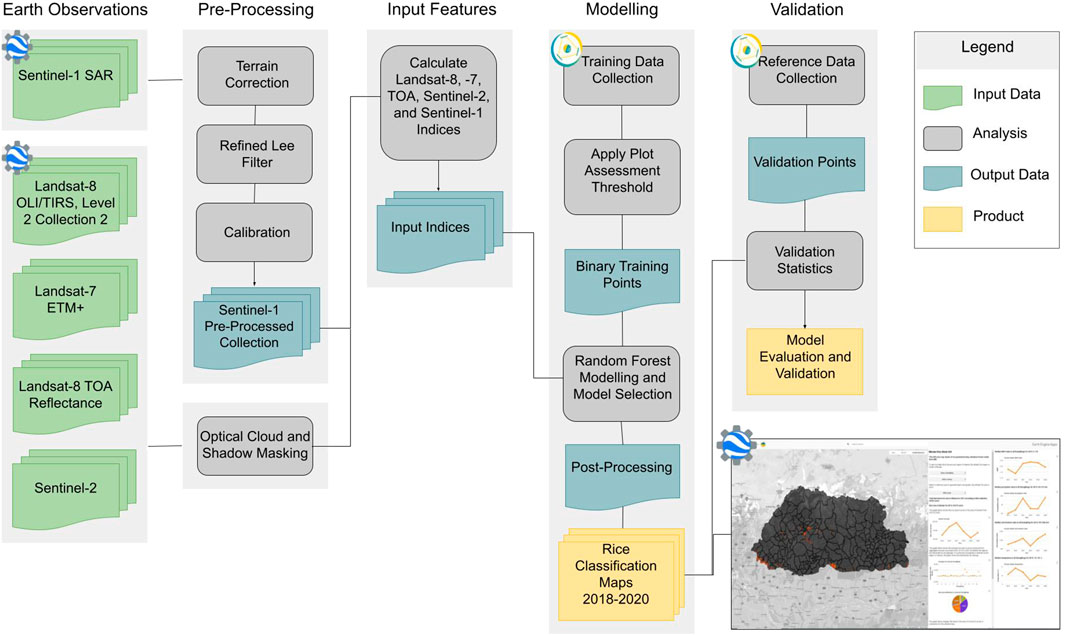
FIGURE 2. Agricultural classification and estimation service (ACES) workflow.

Interpretation of high-resolution NICFI imagery was used to categorize each 30 × 30 m assessment plot as either rice or non-rice (Woodward et al., 2018). The open source software CEO (Saah et al., 2019) allows users to inspect high and very high-resolution data anywhere in the world enabling customized sampling surveys. For all 5,005 assessment plots, a survey within CEO was designed wherein nine equidistant points were bounded within the 30 × 30 m plot to aid the data collection team in categorizing the plot. Each point represented 1/9 of the assessment plot area and required a categorization of rice/non-rice for the survey, resulting in a total of 45,045 responses. Plots that did not have sufficient imagery (e.g., cloud cover) were “flagged” in CEO. Only 1 plot was flagged, resulting in a total of 5,004 usable plots. A team of data collectors classified each assessment unit as either rice or non-rice utilizing the following decision tree approach shown in Figure 3.

FIGURE 3

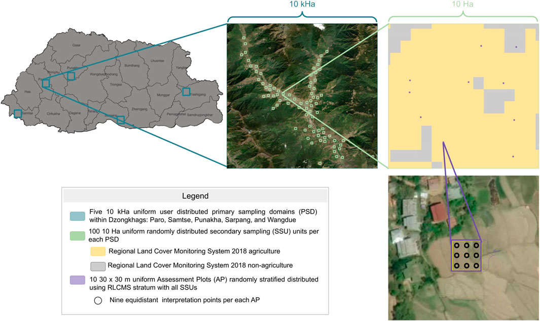
FIGURE 3. Training Sample Design leveraging Google Earth Engine, Collect Earth Online, and SERVIR’s Regional Land Cover Monitoring System.

Preliminary testing of 5,004 assessment plots and subsequent 45,036 points was conducted to identify the plot level binary threshold at distinct ratios. When considering an entire 30 × 30 m assessment plot as rice or non-rice various thresholds starting with less than or equal to (LTE) 2 of the 9 equidistant points were reported as rice were applied. A total of six distinct thresholded training data sets, 2/9, 3/9, 4/9, 5/9, 6/9, and 7/9, where the ratio of mixed focal class was perturbed were investigated.

2.4.1 Independent model validation sample design

To independently assess the performance of the produced models, an additional random stratified sample across Bhutan was employed. This stratification was performed based on the output of the final model for the years 2019 and 2020. Thus, there were two strata for each year, predicted rice and predicted non-rice. For each year, 300 points were randomly generated within each strata resulting in a total of 1,200 points generated. Of these 1,200 plots, 1 was removed due to insufficient imagery for the necessary time period, resulting in a total of 1,199 points used in the independent validation.

Similar to the training sample design aforementioned, Planet NICFI imagery was interpreted using CEO for all 1,199 points. The same dimensions of a 30 × 30 m plot were used for the interpretation. However, in this case, interpreters were instructed to categorize a plot as rice if over 50% of the assessment plot was interpreted to be rice. This data set was leveraged only for the independent model assessment.

2.5 Model

A Random Forest (Breiman, 2001) supervised machine learning model was used for classifying rice. Specifically, this Random Forest algorithm utilized the smileRandomForest function available within GEE and as a method in the ACES system. The Random Forest algorithm is an ensemble-based method where “n” number of decision trees are used to make the final prediction. Random Forest has both classification and regression modes. For the classification mode, the class is determined by the majority of decisions from the ensemble, and for regression the average of the predictions is used. The classification mode was used for this analysis as a binary rice/non-rice output was produced.

2.5.1 Preliminary model testing

A series of preliminary testing efforts were conducted to evaluate the sensitivity and influence of data set inputs and Random Forest model parameters to develop the most robust model by perturbing the following model constituents: Input data, Bag Fraction, Min Leaf Population, Number of Trees, and Variables Per Split.

As aforementioned, the six LTE distinct rice/non-rice thresholds were defined at the plot level, and are referred to as LTE2, LTE3, LTE4, LTE5, LTE6, and LTE7. The bag fraction hyperparameter ranged from 0.5 to 1 at increments of 0.1, resulting in six unique settings. The minimum leaf population ranged from one to five, thus resulting in five unique settings in the preliminary phase. The number of trees ranged from 30–120 at increments of 10, producing 10 unique settings. Finally, the model was set to enable variable splits between null (i.e., no limit) and the total number of input feature bands, in this case 28. As this was a binary state, only two unique settings were produced for these components.

With the series of preliminary tests, a total of 3,600 unique models were generated (Input Data: 6 X Bag fraction: 6 X Min Leaf Population: 5 X Number of Trees: 10 X Variables Per Split X 2). Figure 7 provides a pairwise model performance comparison for each LTE threshold set to each hyperparameter tuning approach. For each of the 3,600 models, 75% of input data was used for model training, and the remaining 25% were separated for testing purposes. These splits were kept the same for each of the 3,600 iterations. Following this series of trials, the best-performing model for each set of LTE iterations are shown in Table 2 in the results section.

TABLE 2

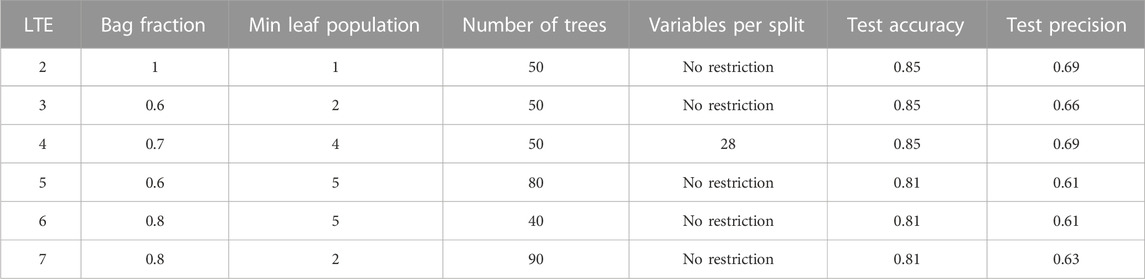
TABLE 2. Reported highest overall accuracy and kappa scores for each LTE model set.

2.6 Post-processing

An additional post-processing step outlined in Figure 4 was added to remove the erroneous model prediction for the final ACES web application portal. Specifically, predicted rice pixels classified as either glacier, bare soil, or bare rock from the corresponding annual RLCMS map were removed as these were evident model over-predictions. Lastly, in GEE, a connected pixel filter set to 30 m was used to remove disconnected or non-contiguous predictions thereby removing clear misclassifications for the final application.

FIGURE 4

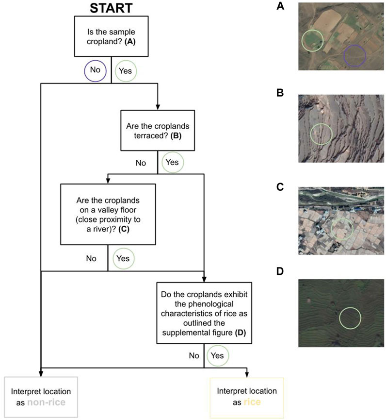
FIGURE 4. Image interpretation decision tree used to categorize assessment plots when collecting training and validation data using Collect Earth Online.

2.7 Accuracy assessment

The following metrics were used to evaluate the cadre of models and perform the independent model evaluation: Overall Accuracy (Eq. 1) Precision (Eq. 2), Recall (Eq 3), F1-score (Eq. 4), and Cohen’s Kappa (Eq. 5).

Using a standard confusion matrix, overall accuracy, precision, and recall are produced. Overall accuracy is the summed number of correctly classified observations divided by the total number of observations. Precision is the ratio of correctly predicted positive observations to the total predicted positive observations, while recall is the ratio of correctly predicted positive observations to all the observations in the focal class. This is often referred to as sensitivity. The F-1 Score (Van Rijsbergen, 1979; Chicco and Jurman, 2020) is then calculated using precision and recall and is the harmonic mean of precision and recall, taking into account both the false positives and false negatives. Cohen’s kappa (Cohen, 1960; Artstein and Poesio, 2008) measures inter-annotator agreement. Kappa is based on the confusion matrix and computes a score that expresses the level of agreement between two annotators.

$OverallAccuracy=TP+TN/TP+TN+FP+FN(1)$

$Precision=TP/TP+FP(2)$

$Recall=TP/TP+FN(3)$

$F1Score=2*\left(Recall*Precision\right)/\left(Recall*Precision\right)(4)$

$Kappa\left(K\right)=\left(p_o-p_e\right)/\left(1-p_e\right)(5)$

Where:

Positive in this case is the presence of rice while Negative refers to a non-rice classification.

TP is the True Positives, when the actual class and the predicted class are both positive.

TN is the True Negatives, when the actual and predicted class are both negative.

FP is the False Positives, when the actual class is negative whereas the predicted class is positive.

FN is the False Negative, when the actual class is positive, but the predicted class is negative.

p_o is the probability of agreement for the focal class

p_e is the expected agreement between both classes when labels are randomly assigned.

3 Results

3.1 Model trials

All of the evaluation metrics were used in ranking and selecting the best-performing model from the set of preliminary trials. For each LTE model set, the best-performing models are displayed in Table 2. From that array of six training LTE data sets, the LTE2 models outperformed the other five data sets. As displayed in Figure 5, and Figure 7 both LTE2 and LTE4 observed overall high median accuracies. However, LTE4 displayed more outliers and thus lower evaluation metrics. Additionally, LTE data sets 5 through 7 displayed lower median accuracies and a wide range of variability. Comparing all 3,600 models collectively through ranking all evaluation metrics, model 555 displayed the highest testing metrics: Overal Accuracy: 85.09%, Precision: 88, Recall: 88, F-1 score: 88, Kappa: 68. Specifically, model 555 was parameterized with the following settings: number of trees: 120, variables per split: no restriction, minimum leaf population: 3, bag fraction: 0.8, and utilized the LTE2 data set for training. This “LTE2 555” model was used for all future analyses. Elevation, S2 MNDWI, and VH ascending were the top three highest important input variables, for the LTE 555 model, as displayed in Figure 6.

FIGURE 5

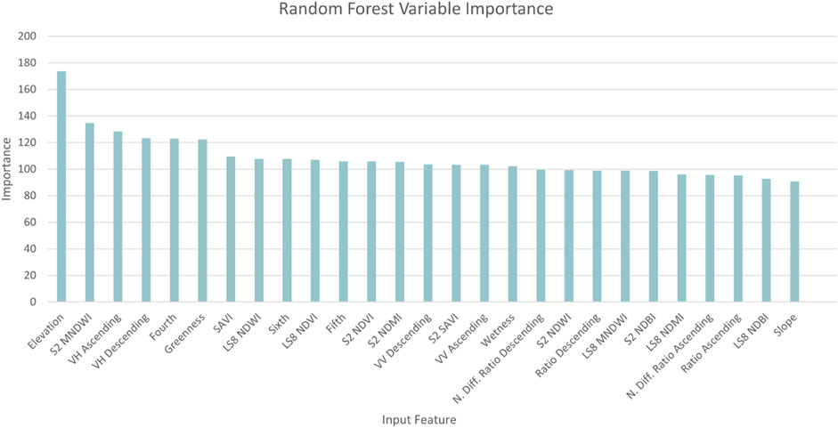
FIGURE 5. LTE2 555 model variable importance.

FIGURE 6

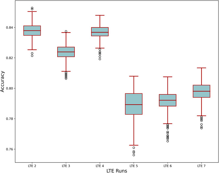
FIGURE 6. Distribution evaluation of the 3,600 model outputs by LTE model sets comparing test accuracies.

For each of the hyperparameter turning model constituents outlined in Figure 7 which displays a high range of variability in test accuracy when investigating bag fraction. The setting of .08 displayed a relatively tighter distribution especially for the LTE2-LTE4 data sets. In general, we observed that an increasing number of trees resulted in improved accuracies most evident in LET 2 and LTE 4. For both the minimum leaf population and variables per split for the 3,600 models and each of the LTE data sets we did not observe a clear advantage for perturbing these model as the test accuracies distributions were consistently expansive.

FIGURE 7

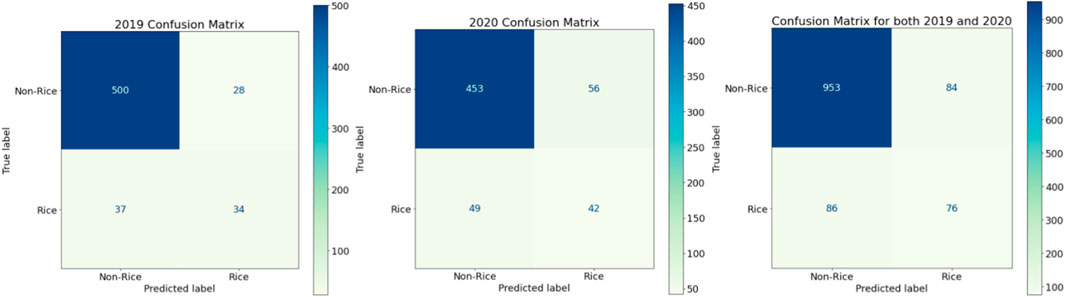
FIGURE 7. Independent validation classification results.

3.2 Independent validation results

An independent validation was conducted utilizing the LTE2 555 model. This effort leverages 1,199 independent validation points with the independently observed rice plots: 62, 98, and non-rice 537, 502, for 2019 and 2020 respectively. Reported metrics for the LTE2 555 model are provided in Table 3 and the confusion matrices for 2019, 2020, and collectively are reported in Figure 8. As evident in Figure 9 and in the reported Table 3, the Precision, Recall, F-1, and Kappa metrics for both 2019 and 2020 were relatively low. The independent validation class balance between rice and non-rice plot was greatly skewed to non-rice. This is a symptom of agriculture being a sparse class, and a 50% threshold for the independent validation at the assessment plot level. Figure 9 displays country level rice prediction for 2020 and outlines the spatial distribution of the independent validation data used for the analysis.

TABLE 3

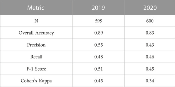
TABLE 3. Independent Validation reported metrics for 2019 and 2020 LTE2 555 model output.

FIGURE 8

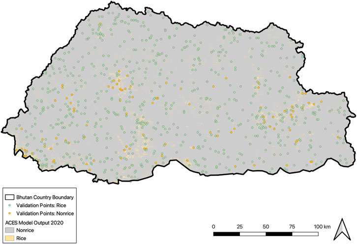
FIGURE 8. Independent validation ACES model output 2020.

FIGURE 9

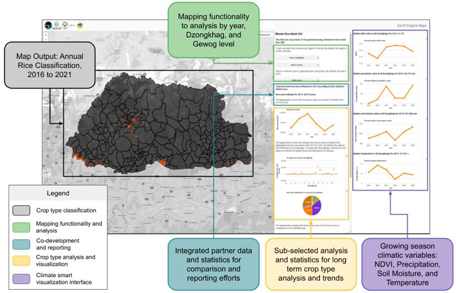
FIGURE 9. Agricultural Classification and Estimation Service (ACES) web application interface outlining crop type classifications, tool functionality, interactive statistics and analysis panel, and finally climate smart visualization interface.

3.3 Application and implementation

Leveraging the methodology available in the ACES software system outlined above, rice extent classification was performed for the growing season (May-October) for the years of 2016–2021, using the LTE2 555 model. These layers are hosted as a Google Cloud Asset along with the geospatial ACES tool to enable end-users and practitioners to query and interact with the data via a web browser. This application allows end-users to visualize 5 years of rice crop extent for the entire country of Bhutan and seamlessly filter by district and sub-district regions. ACES summarizes the predicted annual rice area extent by the filtered region and incorporates the rice statistics reported by Department of Agriculture and the National Statistics Bureau of Bhutan, allowing for direct comparison within the dashboard. Predicted annual rice area gain and/or loss are plotted for all years to evaluate the crop rotation dynamics by a given region. In addition, the ACES application has a dedicated climate and phenology-focused information panel, displaying soil moisture, accumulated precipitation, air temperature at 2 m above the surface, and the median NDVI for the user-selected regions and years as shown Supplementary Figure S2. Both the soil moisture and precipitation data sets are acquired from the University of Idaho TerraClimate group (Abatzoglou et al., 2018). The temperature data set is from the European Centre for Medium-Range Weather Forecasts (ECMWF) European ReAnalysis 5 (ERA5) project (Muñoz-Sabater et al., 2021). Lastly, the median NDVI is derived using the same process outlined in 2.3. Each of these data sets are available in GEE and these EO and model data sets were co-designed as they are relevant climactic and phenological indicators for informing crop condition.

Due to the co-developed nature of the ACES tool, it has the ability to complement decision-makers’ efforts by providing consistent, efficient metrics for reporting at the sub-district level. ACES provides key agriculturally relevant data quantification as well as climate smart and streamlined EO solutions into a single dashboard to inform a more resilient food security planning process. The focus on developing geospatial capacity and co-development of platforms aligns with the nation’s intent and drive to go digital, and at the same time the application provides option for data triangulation. Lastly, the ACES web application and software package are both open source and freely available and the partners are working to integrate the ACES system into the Renewable Natural Resources (RNR) statistics and by the Policy and Planning Division (PPD) for direct use.

4 Discussion

The creation and co-development of a geospatial application, when well designed, has the ability to enable users to leverage previously esoteric and inaccessible data sources and solutions. Specifically, a geospatial service well positioned within an organization’s decision-making process has the ability to drastically improve efficiency be that by creating centralized databases, moving previous tabular data into a spatial context and data structure, or integrating an array of data sources, such as climactic or biogeophysical information. With a lower barrier for making data-informed decisions, from a co-developed service, institutions and organizations are more well positioned to combat existing and future environmental challenges. As the ACES application and software are available, significant monitoring, evaluation, and learning (MEL) will be required to assess the impact stemming from this climate-smart tailored geospatial application.

As part of the co-creation of the ACES system, crucial data processing steps, limitations, and caveats were identified. Specifically, Bhutan is a country that experiences a high percentage of cloud cover, which in turn may affect the quantity and quality of the optical imagery employed for the modeling efforts during the growing season. From the set of 3,600 preliminary model Elevation, S2 MNDWI, and VH Ascending were consistently reported as the highest percent contribution for all 28 input features to the model, with elevation being the most important input variable for all LTE sets. The S2 MNDWI optical imagery input variable remained a consistently important variable indicating that the median compositing approach for the growing season helped to alleviate the reduced number of observations due to cloudy conditions. Additionally, significant pre-processing of S-1 was required to combat the common topographic errors when employing the S-1 GRD products. These additional steps significantly increased the processing and technical data manipulation. However, this resulted in a vastly improved data set, as VH Ascending was consistently an important variable in the LTE sets. We would recommend researchers and practitioners to pursue this level of additional S-1 pre-processing, especially in extremely mountainous terrain such as Bhutan.

A standardized sampling protocol for surveying and collecting training data was also developed. The sampling protocol, utilizing CEO, is a system that will enable stakeholders to replicate surveys for annual data collection. See the Supporting Material for an example CEO standardized survey. As part of the preliminary testing, a significant focus of the analysis centered on evaluating inherently heterogeneous 30 × 30 m assessment plots. As Bhutan has extremely complex terrain, terraced fields are especially challenging when modeling due to the constrained field sizes and mixed land cover classes within plots. The evaluation of each of the LTE sets allowed a clearer understanding regarding the heterogeneity tolerance level at the plots. With LTE2 555 being outlined as the best reported heterogeneity split, where at least two of the nine equidistant points were observed as rice, this suggests a greater preference for class balance over homogeneous plots. More testing with varied plot sizes and/or greater survey population size will better elucidate this trend in future research. However, this flexibility in the sampling design enables end-users to moderate their own heterogeneity tolerance threshold at the plot level, which is critical in extremely mountainous and diverse landscapes. This standardized framework for field data collection is critical in that it greatly reduces the level of effort needed for generating remote sensing-oriented field collections and systematizes the spatial data for reporting and further analysis.

Lastly, a robust model was developed through a rigorous series of preliminary testing and independent validation. The series of hyperparameter testing conducted in the preliminary trials helped to elucidate the most optimized parameterization and lended useful insight as to the most impactful tuning approaches on model performance. Specifically the hyperparameter bag fraction and number of trees model settings were identified as the most informative settings. Specifically a bag fraction at 0.8 for the LTE 2 data set displayed the lowest test accuracy variability and is a recommended tuning setting for future implementations using ACES. Additionally, we observed the correlation between the increased number of trees and increasing test accuracies thereby we conclude employing a high number of trees for training purposes when leveraging the ACES system. The other model hyperparameter, minimum leaf population and variables per split, did not offer a clear accuracy distinction.

From this robust preliminary model trial effort, the best performing model was identified: LTE2 555. This random forest model provided 2020 evaluation metrics for Overall Accuracy: 85%, 83%; Precision: .88, .43; Recall: .88, .46; F-1 score: .88, .45; and Kappa: .68 .34 for test and independent validation respectively. The accuracy remained relatively high between the testing and the independent validation phases. However there was a reduction of Precision, Recall, F-1 score, and Kappa between these two distinct phases. We surmise that these decreased evaluation metrics stem from the independent validation rice/non-rice imbalance. For instance, for 2020 of the 600 distributed plots 453 were interpreted as non-rice seen in Figure 7. This imbalance can greatly affect the utility of the final maps. Specifically, the independent evaluation metrics support that the model is very accurate, however this accuracy is most telling for detecting non-rice instances due to the lack of independent validation rice observations and thereby lower evaluation metrics. Therefore future independent validation approaches will look to also utilize the nine equidistant assessment plot interpretation approach, as a threshold of 50% as identified through the LTE trials is unsuitable for the complex terrain of Bhutan. With future work planned to incorporate a more balanced independent validation approach we expect metrics like Precision, Recall, F-1, and Kappa to improve for this distinct phase. As outlined in the paper, the methodologies employed for testing and developing the LTE2 555 Random Forest model will enable stakeholders, researchers, and practitioners to leverage the classification framework for future rice mapping efforts. With this clear description of the modeling framework, we hope that this will greatly reduce the barrier to future applications leveraging the software package ACES.

4.1 Future work

Developing a MEL assessment to evaluate the impact of the ACES application will be critical in the coming years. Specifically, exploring the value of this framework from the stakeholder perspective will allow for future iterations and an improved ACES application coupled with geospatial capacity-building efforts.

In future studies, we will investigate the data collection team agreement strategy for scaled data collection, especially surrounding independent validation efforts. Due to a small number of misinterpreted training points, we will further stress a greater rigor for future training sampling collection efforts. Additionally, we recommend future CEO data collection efforts to specifically incorporate more locations with glaciers and/or perennial snow as these were observed sparse classes. This increased incorporation of landscape diversity in the training data set could strengthen the model performance. Additionally for future preliminary model testing we will explore perturbing the number of trees far beyond the highest setting of 120. Identifying the test accuracy performance peak is warranted in future implementations of the ACES system.

As the ACES application focuses solely on rice classification, as it was considered the highest priority by partners, all development focused on this key species. However, the ACES software package is highly flexible and has the ability to be redeployed geographically and/or adjusted to focus on a different focal crop type. Exploring the sensitivity of the LTE2 555 model settings both in different geographies and on new crop types will be a future step for this research group. Additionally, partners will plan to use the ACES application for ground thruthing to assess the tool, as part of their annual field surveys.

Data availability statement

The datasets presented in this study can be found in online repositories. The names of the repository/repositories and accession number(s) can be found in the article/Supplementary Material.

Author contributions

Conceptualization, TM, BB, FM, AP, and TW; methodology, TM, BB, FM, MM, KW, SJ, MK, AP, TW, LP, ND, CT, and WD; software, TM, BB, and WD; validation, TM, BB, FM, MM, KW, SJ, and MK; formal analysis, TM and BB; investigation, TM and BB; resources, TM, BB, FM, MM, KW, SJ, MK, AP, LP, and WD; data curation, TM, BB, FM, MM, TW, LP, ND, CT, and WD; writing—original draft preparation, TM, BB, FM, MM, KW, SJ, and MK; writing—review and editing, TM, BB, FM, MM, KW, SJ, MK, AP, TW, LP, ND, CT, and WD visualization, TM, BB, FM, MM, KW, SJ, and MK; supervision, TM; project administration, TM; funding acquisition, TM. All authors have read and agreed to the published version of the manuscript.

Funding

This research was funded by the joint US Department of State and NASA through the Inter-Agency Agreement: 1931CQ19Y000. Additionally, this research was funded through the US Agency for International Development (USAID) and NASA initiative Cooperative Agreement Number: AID486-A-14-00002. Individuals affiliated with the University of Alabama in Huntsville (UAH) are funded through the NASA Applied Sciences Capacity Building Program, NASA Cooperative Agreement: 80MSFC22M004.

Conflict of interest

The authors declare that the research was conducted in the absence of any commercial or financial relationships that could be construed as a potential conflict of interest.

Publisher’s note

All claims expressed in this article are solely those of the authors and do not necessarily represent those of their affiliated organizations, or those of the publisher, the editors and the reviewers. Any product that may be evaluated in this article, or claim that may be made by its manufacturer, is not guaranteed or endorsed by the publisher.

Supplementary material

The Supplementary Material for this article can be found online at: https://www.frontiersin.org/articles/10.3389/fenvs.2023.1137835/full#supplementary-material

References

Abatzoglou, J. T., Dobrowski, S. Z., Parks, S. A., and Hegewisch, K. C. (2018). Terraclimate, a high-resolution global dataset of monthly climate and climatic water balance from 1958–2015. Sci. data 5, 170191–170212. doi:10.1038/sdata.2017.191

PubMed Abstract | CrossRef Full Text | Google Scholar

Agriculture, B. M. and Forests (1992). Ministry of agriculture and forests: Renewable natural resources research strategy and plan.

Google Scholar

Artstein, R., and Poesio, M. (2008). Inter-coder agreement for computational linguistics. Comput. Linguist. 34, 555–596. doi:10.1162/coli.07-034-r2

CrossRef Full Text | Google Scholar

Assembly, U. G. (2015). Transforming our world: The 2030 agenda for sustainable development. 21 october 2015. Retrieved from.

Google Scholar

Baig, M. H. A., Zhang, L., Shuai, T., and Tong, Q. (2014). Derivation of a tasselled cap transformation based on landsat 8 at-satellite reflectance. Remote Sens. Lett. 5, 423–431. doi:10.1080/2150704x.2014.915434

CrossRef Full Text | Google Scholar

Bey, A., Sánchez-Paus Díaz, A., Maniatis, D., Marchi, G., Mollicone, D., Ricci, S., et al. (2016). Collect Earth: Land use and land cover assessment through augmented visual interpretation. Remote Sens. 8, 807. doi:10.3390/rs8100807

CrossRef Full Text | Google Scholar

Breiman, L. (2001). Random forests. Mach. Learn. 45, 5–32. doi:10.1023/a:1010933404324

CrossRef Full Text | Google Scholar

Brisco, B., Kapfer, M., Hirose, T., Tedford, B., and Liu, J. (2011). Evaluation of c-band polarization diversity and polarimetry for wetland mapping. Can. J. Remote Sens. 37, 82–92. doi:10.5589/m11-017

CrossRef Full Text | Google Scholar

Brown, M., De Beurs, K., and Marshall, M. (2012). Global phenological response to climate change in crop areas using satellite remote sensing of vegetation, humidity and temperature over 26 years. Remote Sens. Environ. 126, 174–183. doi:10.1016/j.rse.2012.08.009

CrossRef Full Text | Google Scholar

Bruggeman, D., Meyfroidt, P., and Lambin, E. F. (2016). Forest cover changes in Bhutan: Revisiting the forest transition. Appl. Geogr. 67, 49–66. doi:10.1016/j.apgeog.2015.11.019

CrossRef Full Text | Google Scholar

Bureau, B. N. S. (2021). Bhutan national statistics bureau agriculture-statistics 2021.

Google Scholar

Bureau, B. N. S. (2022). Bhutan national statistics bureau: Statistical yearbook of Bhutan.

Google Scholar

Carrasco, L., O’Neil, A. W., Morton, R. D., and Rowland, C. S. (2019). Evaluating combinations of temporally aggregated sentinel-1, sentinel-2 and landsat 8 for land cover mapping with Google Earth engine. Remote Sens. 11, 288. doi:10.3390/rs11030288

CrossRef Full Text | Google Scholar

Chander, G., Markham, B. L., and Helder, D. L. (2009). Summary of current radiometric calibration coefficients for landsat mss, tm, etm+, and eo-1 ali sensors. Remote Sens. Environ. 113, 893–903. doi:10.1016/j.rse.2009.01.007

CrossRef Full Text | Google Scholar

Chen, C., Son, N., Chen, C., Chang, L., and Chiang, S. (2016). Rice crop mapping using sentinel-1a phenological metrics. Int. Archives Photogrammetry, Remote Sens. Spatial Inf. Sci. 41.

CrossRef Full Text | Google Scholar

Chhogyel, N., and Kumar, L. (2018). Climate change and potential impacts on agriculture in Bhutan: A discussion of pertinent issues. Agric. Food Secur. 7, 79–13. doi:10.1186/s40066-018-0229-6

CrossRef Full Text | Google Scholar

Chicco, D., and Jurman, G. (2020). The advantages of the matthews correlation coefficient (mcc) over f1 score and accuracy in binary classification evaluation. BMC genomics 21, 6–13. doi:10.1186/s12864-019-6413-7

PubMed Abstract | CrossRef Full Text | Google Scholar

Chong, L., Liu, H.-j., Lu, L.-p., Liu, Z.-r., Kong, F.-c., and Zhang, X.-l. (2021). Monthly composites from sentinel-1 and sentinel-2 images for regional major crop mapping with Google Earth engine. J. Integr. Agric. 20, 1944–1957. doi:10.1016/s2095-3119(20)63329-9

CrossRef Full Text | Google Scholar

Choudhury, I., and Chakraborty, M. (2004). Analysis of temporal sar and optical data for rice mapping. J. Indian Soc. Remote Sens. 32, 373–385. doi:10.1007/bf03030862

CrossRef Full Text | Google Scholar

Cohen, J. (1960). A coefficient of agreement for nominal scales. Educ. Psychol. Meas. 20, 37–46. doi:10.1177/001316446002000104

CrossRef Full Text | Google Scholar

Crist, E. P., and Kauth, R. (1986). The tasseled cap de-mystified. Photogrammetric Eng. remote Sens. 52.

Google Scholar

Dhu, T., Dunn, B., Lewis, B., Lymburner, L., Mueller, N., Telfer, E., et al. (2017). Digital Earth Australia–unlocking new value from Earth observation data. Big Earth Data 1, 64–74. doi:10.1080/20964471.2017.1402490

CrossRef Full Text | Google Scholar

Dong, J., Xiao, X., Menarguez, M. A., Zhang, G., Qin, Y., Thau, D., et al. (2016). Mapping paddy rice planting area in northeastern Asia with landsat 8 images, phenology-based algorithm and Google Earth engine. Remote Sens. Environ. 185, 142–154. doi:10.1016/j.rse.2016.02.016

PubMed Abstract | CrossRef Full Text | Google Scholar

Farr, T. G., Rosen, P. A., Caro, E., Crippen, R., Duren, R., Hensley, S., et al. (2007). The shuttle radar topography mission. Rev. Geophys. 45. doi:10.1029/2005rg000183

CrossRef Full Text | Google Scholar

Flores-Anderson, A. I., Herndon, K. E., Thapa, R. B., and Cherrington, E. (2019). The SAR handbook: Comprehensive methodologies for forest monitoring and biomass estimation. Tech. Rep.

Google Scholar

Frankel-Reed, J. (2018). “Reflecting on a decade of collaboration between nasa and usaid: Deriving value from space for international development,” in Yearbook on Space policy 2016 (Springer), 163–174.

CrossRef Full Text | Google Scholar

Ghimiray, M. (2012). An analysis of rice varietal improvement and adoption rate by farmers in Bhutan. J. Renew. Nat. Resour. Bhutan 8, 13–24.

Google Scholar

Gilani, H., Shrestha, H. L., Murthy, M., Phuntso, P., Pradhan, S., Bajracharya, B., et al. (2015). Decadal land cover change dynamics in Bhutan. J. Environ. Manag. 148, 91–100. doi:10.1016/j.jenvman.2014.02.014

CrossRef Full Text | Google Scholar

Giuliani, G., Nativi, S., Obregon, A., Beniston, M., and Lehmann, A. (2017). Spatially enabling the global framework for climate services: Reviewing geospatial solutions to efficiently share and integrate climate data and information. Clim. Serv. 8, 44–58. doi:10.1016/j.cliser.2017.08.003

CrossRef Full Text | Google Scholar

Gomes, V. C., Queiroz, G. R., and Ferreira, K. R. (2020). An overview of platforms for big Earth observation data management and analysis. Remote Sens. 12, 1253. doi:10.3390/rs12081253

CrossRef Full Text | Google Scholar

Gorelick, N. (2013). “Google Earth engine,” in EGU general assembly conference abstracts (American Geophysical Union Vienna, Austria) 15, 11997.

Google Scholar

Griggs, D., Stafford-Smith, M., Gaffney, O., Rockström, J., Öhman, M. C., Shyamsundar, P., et al. (2013). Sustainable development goals for people and planet. Nature 495, 305–307. doi:10.1038/495305a

PubMed Abstract | CrossRef Full Text | Google Scholar

Gumma, M. K., Nelson, A., Thenkabail, P. S., and Singh, A. N. (2011). Mapping rice areas of south Asia using modis multitemporal data. J. Appl. remote Sens. 5, 053547. doi:10.1117/1.3619838

CrossRef Full Text | Google Scholar

Huang, C., Chen, Y., Zhang, S., and Wu, J. (2018a). Detecting, extracting, and monitoring surface water from space using optical sensors: A review. Rev. Geophys. 56, 333–360. doi:10.1029/2018rg000598

CrossRef Full Text | Google Scholar

Huang, S., Tang, L., Hupy, J. P., Wang, Y., and Shao, G. (2021). A commentary review on the use of normalized difference vegetation index (ndvi) in the era of popular remote sensing. J. For. Res. 32, 1–6. doi:10.1007/s11676-020-01155-1

CrossRef Full Text | Google Scholar

Huang, W., DeVries, B., Huang, C., Lang, M. W., Jones, J. W., Creed, I. F., et al. (2018b). Automated extraction of surface water extent from sentinel-1 data. Remote Sens. 10, 797. doi:10.3390/rs10050797

CrossRef Full Text | Google Scholar

Huete, A. R. (1988). A soil-adjusted vegetation index (savi). Remote Sens. Environ. 25, 295–309. doi:10.1016/0034-4257(88)90106-x

CrossRef Full Text | Google Scholar

Hydrology, N. C. and Meteorology (2019). National center for hydrology and meteorology: Analysis of historical climate and climate projection for Bhutan.

Google Scholar

Hydrology, N. C. and Meteorology (2020). National center for hydrology and meteorology:Bhutan state of the climate 2020.

Google Scholar

Jiang, R., Sanchez-Azofeifa, A., Laakso, K., Xu, Y., Zhou, Z., Luo, X., et al. (2021). Cloud cover throughout all the paddy rice fields in guangdong, China: Impacts on sentinel 2 msi and landsat 8 oli optical observations. Remote Sens. 13, 2961. doi:10.3390/rs13152961

CrossRef Full Text | Google Scholar

Katwal, T. (2013). “Multiple cropping in bhutanese agriculture: Present status and opportunities,” in Regional consultative meeting on popularizing multiple cropping innovations as a means to raise productivity and farm income in SAARC countries, peradeniya, kandy, srilanka.

Google Scholar

Kauth, R. J., and Thomas, G. (1976). “The tasselled cap–a graphic description of the spectral-temporal development of agricultural crops as seen by landsat,” in LARS symposia, 159.

Google Scholar

Kyere, I., Astor, T., Graß, R., and Wachendorf, M. (2020). Agricultural crop discrimination in a heterogeneous low-mountain range region based on multi-temporal and multi-sensor satellite data. Comput. Electron. Agric. 179, 105864. doi:10.1016/j.compag.2020.105864

CrossRef Full Text | Google Scholar

Landsat, U. (2022). Landsat 8–9 collection 2 (c2) level 2 science product (l2sp) guide. NC, USA: United States Geological Survey: Asheville, 1–42.

Google Scholar

Lasko, K., Vadrevu, K. P., Tran, V. T., and Justice, C. (2018). Mapping double and single crop paddy rice with sentinel-1a at varying spatial scales and polarizations in hanoi, vietnam. IEEE J. Sel. Top. Appl. Earth Observations Remote Sens. 11, 498–512. doi:10.1109/jstars.2017.2784784

CrossRef Full Text | Google Scholar

Lee, J.-S., Wen, J.-H., Ainsworth, T. L., Chen, K.-S., and Chen, A. J. (2008). Improved sigma filter for speckle filtering of sar imagery. IEEE Trans. Geoscience Remote Sens. 47, 202–213.

Google Scholar

Lemajic, B. V. S., and Åstrand, P. J. (2018). New sensors benchmark report on planetscope.

Google Scholar

Li, P., Feng, Z., and Xiao, C. (2018). Acquisition probability differences in cloud coverage of the available landsat observations over mainland southeast Asia from 1986 to 2015. Int. J. Digital Earth 11, 437–450. doi:10.1080/17538947.2017.1327619

CrossRef Full Text | Google Scholar

Main-Knorn, M., Pflug, B., Louis, J., Debaecker, V., Müller-Wilm, U., and Gascon, F. (2017). “Sen2cor for sentinel-2,” in Image and signal processing for remote sensing XXIII (SPIE), 10427, 37–48.

CrossRef Full Text | Google Scholar

Mayer, T., Poortinga, A., Bhandari, B., Nicolau, A. P., Markert, K., Thwal, N. S., et al. (2021). Deep learning approach for sentinel-1 surface water mapping leveraging Google Earth engine. ISPRS Open J. Photogrammetry Remote Sens. 2, 100005. doi:10.1016/j.ophoto.2021.100005

CrossRef Full Text | Google Scholar

McFeeters, S. K. (1996). The use of the normalized difference water index (ndwi) in the delineation of open water features. Int. J. remote Sens. 17, 1425–1432. doi:10.1080/01431169608948714

CrossRef Full Text | Google Scholar

McNairn, H., and Brisco, B. (2004). The application of c-band polarimetric sar for agriculture: A review. Can. J. Remote Sens. 30, 525–542. doi:10.5589/m03-069

CrossRef Full Text | Google Scholar

Muñoz-Sabater, J., Dutra, E., Agustí-Panareda, A., Albergel, C., Arduini, G., Balsamo, G., et al. (2021). Era5-land: A state-of-the-art global reanalysis dataset for land applications. Earth Syst. Sci. Data 13, 4349–4383. doi:10.5194/essd-13-4349-2021

CrossRef Full Text | Google Scholar

Nativi, S., Santoro, M., Giuliani, G., and Mazzetti, P. (2019). Towards a knowledge base to support global change policy goals. Int. J. digital earth 13, 188–216. doi:10.1080/17538947.2018.1559367

CrossRef Full Text | Google Scholar

Ndikumana, E., Ho Tong Minh, D., Dang Nguyen, H. T., Baghdadi, N., Courault, D., Hossard, L., et al. (2018). Estimation of rice height and biomass using multitemporal sar sentinel-1 for camargue, southern France. Remote Sens. 10, 1394. doi:10.3390/rs10091394

CrossRef Full Text | Google Scholar

Nelson, A., Setiyono, T., Rala, A. B., Quicho, E. D., Raviz, J. V., Abonete, P. J., et al. (2014). Towards an operational sar-based rice monitoring system in Asia: Examples from 13 demonstration sites across Asia in the riice project. Remote Sens. 6, 10773–10812. doi:10.3390/rs61110773

CrossRef Full Text | Google Scholar

Neuhoff, D., Tashi, S., Rahmann, G., and Denich, M. (2014). Organic agriculture in Bhutan: Potential and challenges. Org. Agric. 4, 209–221. doi:10.1007/s13165-014-0075-1

CrossRef Full Text | Google Scholar

Nguyen, T. T. H., De Bie, C., Ali, A., Smaling, E., and Chu, T. H. (2012). Mapping the irrigated rice cropping patterns of the mekong delta, vietnam, through hyper-temporal spot ndvi image analysis. Int. J. remote Sens. 33, 415–434. doi:10.1080/01431161.2010.532826

CrossRef Full Text | Google Scholar

Ni, R., Tian, J., Li, X., Yin, D., Li, J., Gong, H., et al. (2021). An enhanced pixel-based phenological feature for accurate paddy rice mapping with sentinel-2 imagery in Google Earth engine. ISPRS J. Photogrammetry Remote Sens. 178, 282–296. doi:10.1016/j.isprsjprs.2021.06.018

CrossRef Full Text | Google Scholar

Oguro, Y., Suga, Y., Takeuchi, S., Ogawa, M., Konishi, T., and Tsuchiya, K. (2001). Comparison of sar and optical sensor data for monitoring of rice plant around hiroshima. Adv. Space Res. 28, 195–200. doi:10.1016/s0273-1177(01)00345-3

CrossRef Full Text | Google Scholar

Ohsawa, M. (1987). Life zone ecology of the Bhutan Himalaya. Laboratory of Ecology, Chiba University Chiba, Japan.

Google Scholar

Olofsson, P., Foody, G. M., Herold, M., Stehman, S. V., Woodcock, C. E., and Wulder, M. A. (2014). Good practices for estimating area and assessing accuracy of land change. Remote Sens. Environ. 148, 42–57. doi:10.1016/j.rse.2014.02.015

CrossRef Full Text | Google Scholar

Orynbaikyzy, A., Gessner, U., and Conrad, C. (2019). Crop type classification using a combination of optical and radar remote sensing data: A review. Int. J. remote Sens. 40, 6553–6595. doi:10.1080/01431161.2019.1569791

CrossRef Full Text | Google Scholar

O’Shea, K., LaRoe, J., Vorster, A., Young, N., Evangelista, P., Mayer, T., et al. (2020). Improved remote sensing methods to detect northern wild rice (zizania palustris l.). Remote Sens. 12, 3023. doi:10.3390/rs12183023

CrossRef Full Text | Google Scholar

Park, S., Im, J., Park, S., Yoo, C., Han, H., and Rhee, J. (2018). Classification and mapping of paddy rice by combining landsat and sar time series data. Remote Sens. 10, 447. doi:10.3390/rs10030447

CrossRef Full Text | Google Scholar

Poortinga, A., Thwal, N. S., Khanal, N., Mayer, T., Bhandari, B., Markert, K., et al. (2021). Mapping sugarcane in Thailand using transfer learning, a lightweight convolutional neural network, nicfi high resolution satellite imagery and Google Earth engine. ISPRS Open J. Photogrammetry Remote Sens. 1, 100003. doi:10.1016/j.ophoto.2021.100003

CrossRef Full Text | Google Scholar

Potin, P., Bargellini, P., Laur, H., Rosich, B., and Schmuck, S. (2012). “Sentinel-1 mission operations concept,” in 2012 IEEE international geoscience and remote sensing symposium (IEEE), 1745–1748.

CrossRef Full Text | Google Scholar

Reiche, J. (2015). Combining SAR and optical satellite image time series for tropical forest monitoring. Wageningen University and Research. Ph.D. thesis.

Google Scholar

Rouse, J. W., Haas, R. H., Schell, J., and Deering, D. (1973). Monitoring the vernal advancement and retrogradation (green wave effect) of natural vegetation. Tech. Rep.

Google Scholar

Saah, D., Johnson, G., Ashmall, B., Tondapu, G., Tenneson, K., Patterson, M., et al. (2019). Collect Earth: An online tool for systematic reference data collection in land cover and use applications. Environ. Model. Softw. 118, 166–171. doi:10.1016/j.envsoft.2019.05.004

CrossRef Full Text | Google Scholar

Schmidt, G., Jenkerson, C. B., Masek, J., Vermote, E., and Gao, F. (2013). Landsat ecosystem disturbance adaptive processing system (ledaps) algorithm description.

Google Scholar

Searby, N. D., Irwin, D., and Kim, T. (2019). “Servir: Leveraging the expertise of a space agency and a development agency to increase impact of Earth observation in the developing world,” in International astronautical congress (TAC). MSFC-E-DAA-TN73625.

Google Scholar

Singha, M., Dong, J., Zhang, G., and Xiao, X. (2019). High resolution paddy rice maps in cloud-prone Bangladesh and northeast India using sentinel-1 data. Sci. data 6, 26–10. doi:10.1038/s41597-019-0036-3

PubMed Abstract | CrossRef Full Text | Google Scholar

Small, D. (2011). Flattening gamma: Radiometric terrain correction for sar imagery. IEEE Trans. Geoscience Remote Sens. 49, 3081–3093. doi:10.1109/tgrs.2011.2120616

CrossRef Full Text | Google Scholar

Statistics, N. B (2012). Poverty analysis report. national bureau of statistics. royal government of bhutan.

Google Scholar

Steele-Dunne, S. C., McNairn, H., Monsivais-Huertero, A., Judge, J., Liu, P.-W., and Papathanassiou, K. (2017). Radar remote sensing of agricultural canopies: A review. IEEE J. Sel. Top. Appl. Earth Observations Remote Sens. 10, 2249–2273. doi:10.1109/jstars.2016.2639043

CrossRef Full Text | Google Scholar

Stehman, S. (2005). Comparing estimators of gross change derived from complete coverage mapping versus statistical sampling of remotely sensed data. Remote Sens. Environ. 96, 466–474. doi:10.1016/j.rse.2005.04.002

CrossRef Full Text | Google Scholar

Talukdar, S., Singha, P., Mahato, S., Pal, S., Liou, Y.-A., Rahman, A., et al. (2020). Land-use land-cover classification by machine learning classifiers for satellite observations—A review. Remote Sens. 12, 1135. doi:10.3390/rs12071135

CrossRef Full Text | Google Scholar

Tamiminia, H., Salehi, B., Mahdianpari, M., Quackenbush, L., Adeli, S., and Brisco, B. (2020). Google Earth engine for geo-big data applications: A meta-analysis and systematic review. ISPRS J. Photogrammetry Remote Sens. 164, 152–170. doi:10.1016/j.isprsjprs.2020.04.001

CrossRef Full Text | Google Scholar

Tashi, D. (2018). Mapping change in rice cultivation using geospatial science in the Paro valley, Bhutan from 1995-2011. Ph.D. thesis, Flinders University, College of Science and Engineering.

Google Scholar

Team, P. (2017). Planet application program interface: In space for life on earth. San Francisco, CA, 40.

Google Scholar

Thapa, R. B., Bajracharya, B., Matin, M. A., Anderson, E., and Epanchin, P. (2021). Service planning approach and its application. A Decade Exp. SERVIR 23.

CrossRef Full Text | Google Scholar

Tobgay, S. (2006). Agriculture diversification in Bhutan. Tech. Rep.

Google Scholar

Tripathi, A., and Tiwari, R. K. (2022). Synergetic utilization of sentinel-1 sar and sentinel-2 optical remote sensing data for surface soil moisture estimation for rupnagar, Punjab, India. Geocarto Int. 37, 2215–2236. doi:10.1080/10106049.2020.1815865

CrossRef Full Text | Google Scholar

Tshewang, S., Sindel, B. M., Ghimiray, M., and Chauhan, B. S. (2016). Weed management challenges in rice (oryza sativa l.) for food security in Bhutan: A review. Crop Prot. 90, 117–124. doi:10.1016/j.cropro.2016.08.031

CrossRef Full Text | Google Scholar

Uddin, K., Matin, M. A., Khanal, N., Maharjan, S., Bajracharya, B., Tenneson, K., et al. (2021). “Regional land cover monitoring system for hindu kush himalaya,” in Earth observation science and applications for risk reduction and enhanced resilience in Hindu Kush Himalaya region (Springer), 103–125.

CrossRef Full Text | Google Scholar

Van Rijsbergen, C. (1979). “Information retrieval: Theory and practice,” in Proceedings of the joint IBM/university of newcastle upon tyne seminar on data base systems, 79.

Google Scholar

Vollrath, A., Mullissa, A., and Reiche, J. (2020). Angular-based radiometric slope correction for sentinel-1 on Google Earth engine. Remote Sens. 12, 1867. doi:10.3390/rs12111867

CrossRef Full Text | Google Scholar

Walcott, S. (2009). Geographical field notes urbanization in Bhutan. Geogr. Rev. 99, 81–93. doi:10.1111/j.1931-0846.2009.tb00419.x

CrossRef Full Text | Google Scholar

Woodward, B. D., Evangelista, P. H., Young, N. E., Vorster, A. G., West, A. M., Carroll, S. L., et al. (2018). Co-Rip: A riparian vegetation and corridor extent dataset for Colorado river basin streams and rivers. ISPRS Int. J. Geo-Information 7, 397. doi:10.3390/ijgi7100397

CrossRef Full Text | Google Scholar

Xiao, X., Boles, S., Frolking, S., Li, C., Babu, J. Y., Salas, W., et al. (2006). Mapping paddy rice agriculture in south and southeast Asia using multi-temporal modis images. Remote Sens. Environ. 100, 95–113. doi:10.1016/j.rse.2005.10.004

CrossRef Full Text | Google Scholar

Xu, H. (2006). Modification of normalised difference water index (ndwi) to enhance open water features in remotely sensed imagery. Int. J. remote Sens. 27, 3025–3033. doi:10.1080/01431160600589179

CrossRef Full Text | Google Scholar

Yang, L., Driscol, J., Sarigai, S., Wu, Q., Chen, H., and Lippitt, C. D. (2022). Google Earth engine and artificial intelligence (ai): A comprehensive review. Remote Sens. 14, 3253. doi:10.3390/rs14143253

CrossRef Full Text | Google Scholar

Zha, Y., Gao, J., and Ni, S. (2003). Use of normalized difference built-up index in automatically mapping urban areas from tm imagery. Int. J. remote Sens. 24, 583–594. doi:10.1080/01431160304987

CrossRef Full Text | Google Scholar

Zhang, Y., Wang, C., Wu, J., Qi, J., and Salas, W. A. (2009). Mapping paddy rice with multitemporal alos/palsar imagery in southeast China. Int. J. Remote Sens. 30, 6301–6315. doi:10.1080/01431160902842391

CrossRef Full Text | Google Scholar

Zhao, R., Li, Y., and Ma, M. (2021). Mapping paddy rice with satellite remote sensing: A review. Sustainability 13, 503. doi:10.3390/su13020503

CrossRef Full Text | Google Scholar