Land development and road salt usage drive long-term changes in major-ion chemistry of streamwater in six exurban and suburban watersheds, southeastern Pennsylvania, 1999–2019

1 Introduction

Recent studies in urbanized areas of northern regions have documented the occurrence of the “freshwater salinization syndrome (FSS),” a watershed-scale increase of salinity and delivery of major ions and metals over time (Bäckström et al., 2004; Dugan et al., 2017; Kaushal et al., 2017; Moore et al., 2017; Bird et al., 2018; Haq et al., 2018; Kaushal et al., 2018; Kaushal et al., 2019; Dugan et al., 2020; Kaushal et al., 2021). In regions affected by roadway deicing application, there have been documented increases of Na⁺ and Cl⁻ in rivers and streams (Interlandi and Crockett, 2003; Kaushal et al., 2005; Kelly et al., 2008; Dailey et al., 2014; Moore et al., 2017). These observed increases are often greatest in watersheds with the highest amounts of impervious surface cover (ISC) and where road deicing salts, which are mainly NaCl but may also contain small amounts of CaCl₂ and MgCl₂, have been applied for decades (Kaushal et al., 2005; Dailey et al., 2014; Corsi et al., 2015; Moore et al., 2020; Rossi et al., 2022). Na⁺ and Cl⁻ concentrations in surface waters are often highest in winter months and early spring when roadway runoff enters streams as overland flow either directly or via storm drains (Interlandi and Crockett, 2003; Kaushal et al., 2005; Steele et al., 2010; Kelly et al., 2012; Corsi et al., 2015; Moore et al., 2017). However, road salt runoff can also infiltrate roadside soils and leach into groundwater. This contaminated groundwater is then discharged into streams year round as baseflow, leading to elevated salt concentrations during summer and fall (Kaushal et al., 2005; Kelly et al., 2008; Kelly et al., 2012; Robinson et al., 2017; Snodgrass et al., 2017).

The corresponding influx of Na⁺ to the subsurface can induce reverse cation exchange reactions, whereby abundant Na⁺ may displace more strongly bound calcium (Ca²⁺), magnesium (Mg²⁺), and potassium (K⁺) from negatively charged mineral surfaces (Rhodes et al., 2001; Martínez and Bocanegra, 2002; Bird et al., 2018; Haq et al., 2018; Schuler and Relyea, 2018; Askri et al., 2022). Once these cations are displaced, there is a higher likelihood that they will leach into waterways via baseflow. As a consequence, many streams in the northeastern and midwestern United States, where road salt is applied, also exhibit increasing concentrations of Ca²⁺, Mg²⁺, and K⁺ over time (Bird et al., 2018; Kaushal et al., 2018). Similar to Na⁺ and Cl⁻, concentrations of these cations are more elevated in watersheds with greater percentages of ISC in the upstream areas (Moore et al., 2017). Additionally, increasing Na⁺ concentrations can exacerbate the physical and chemical weathering of concrete infrastructure by salt crystallization, thereby releasing Ca²⁺, sulfate (SO₄^2-), and bicarbonate (HCO₃⁻) to surface waters (Thaulow and Sahu, 2004; Shi et al., 2010; Wright et al., 2011; Kaushal et al., 2014; Moore et al., 2017; Owan and Badawy, 2019). These ions ultimately correspond to the use of crushed limestone (CaCO₃) and gypsum (CaSO₄ · H₂O) as the binding/hydration agents in Portland cement (Lerch, 2008; Lothenbach et al., 2008). Yet, delineating the impacts of road salt driven changes in major ion flux for mixed use watersheds also requires an understanding of other potential sources. For example, elevated export of Ca²⁺ and HCO₃⁻ has been shown in agricultural watersheds affected by lime application (Raymond et al., 2008; Barnes and Raymond, 2009; Kaushal et al., 2018). Additionally, increased SO₄^2- concentrations in agricultural watersheds have been linked to the use of sulfur compounds in fertilizers and soil amendments (Schilling and Wolter, 2001; Spoelstra et al., 2021). From an urban perspective, detergents and disinfectants at wastewater treatment plants (WWTPs) have been identified as sources of Na⁺, Cl⁻, and HCO₃⁻ (Kaushal et al., 2005; Steele and Aitkenhead-Peterson, 2011; Kaushal et al., 2013). Finally, acid rain driven mineral weathering has also been linked to increasing base cation concentrations in northeastern watersheds (Likens et al., 1996; Kaushal et al., 2017).

Regardless of origin, increases of major ion concentrations in streamwater have implications for both human health and infrastructure. With respect to drinking water, the U.S. Environmental Protection Agency (USEPA) established non-enforceable secondary maximum contaminant levels (SMCLs) of 250 mg L^-1 for Cl⁻ (United States Environmental Protection Agency, 2021b) and recommends Na⁺ concentrations not exceed 30–60 mg L^-1; both to avoid adverse effects on taste (USEPA, 2003). However, the USEPA recommends Na⁺ concentrations not exceed 20 mg L^-1 for individuals restricted to a total sodium intake of 500 mg day^-1 (United States Environmental Protection Agency, 2003). Yet, in roadway deicing agent impacted regions, Na⁺ concentrations well in excess of 20 mg L^-1 have been identified in both streamwater samples collected in close proximity to drinking water intakes (Interlandi and Crockett, 2003; Kaushal et al., 2021; Rossi et al., 2022), as well as treated drinking water (Cruz et al., 2022). For example, Cruz et al. (2022) found that wintertime Na⁺ spikes in Philadelphia, Pennsylvania region tap water (up to 126 mg L^-1) contributed between 13.7% and 31.3% to the recommended daily sodium intake limits ingested by adults on non-restricted (2,500 mg day^-1) and “low salt” diets (<1,500 mg day^-1), respectively. Furthermore, studies from other snow affected locales have found a positive association between tap water sodium concentrations and diastolic and/or systolic blood pressure (Hallenbeck et al., 1981; Tuthill and Calabrese, 1981; Talukder et al., 2017).

Elevated Cl⁻ concentrations can also impact drinking water infrastructure and the associated treatment practices. Both the Chloride to Sulfate Mass Ratio (CSMR) and Larson Ratio (LR (chloride + sulfate)/alkalinity) quantify the potential to corrode lead, copper, iron, and steel drinking water distribution networks (Nguyen et al., 2011; Pieper et al., 2017; Stets et al., 2018; United States Environmental Protection Agency, 2022b). For example, CSMR values >0.5 and LR values >1.2 signify enhanced corrosion potential (Edwards and Triantafyllidou, 2007; Agatemor and Okolo, 2008; Nguyen et al., 2011; Masten et al., 2016; Pieper et al., 2017). Previous studies evaluating CSMR and/or LR ratios in streamwater samples collected from roadway deicing agent impacted regions found these ratios are increasing due to both an increase in Cl⁻ inputs from road salt runoff, as well as a decrease in sulfate deposition as a result of more stringent air pollution regulations (National Atmospheric Deposition Program, 1997; Elkin et al., 2016; Bird et al., 2018; Stets et al., 2018; National Atmospheric Deposition Program, 2020).

Increasing corrosivity of source water and drinking water supplies can mobilize metals, such as lead (Pb), resulting in serious impacts to human health, particularly for infants and children. Pb exposure can slow mental development and leave children with lifelong learning disabilities (Cecil et al., 2008; McLaine et al., 2013; Aizer et al., 2018; United States Environmental Protection Agency, 2021a). In adults, Pb exposure can lead to neurological and kidney disorders, as well as high blood pressure (Stewart et al., 2006; Leff et al., 2018). For example, the Flint Water Crisis in Flint, Michigan was partially attributed to a switch of water sources from the more dilute Lake Huron (City of Detroit) to the road salt impacted Flint River (City of Flint). This switch resulted in changes to the CSMR values in treated drinking water from 0.45 for the City of Detroit (Torrice, 2016) to values ranging from 2.8 to 3.8 for the City of Flint (Masten et al., 2016). The corresponding Pb leaching from pipe networks ultimately impacted the children of Flint, with 4.9% showing elevated blood lead levels, an increase from the 2.4% of children with elevated blood lead levels prior to the shift of water sources (Hanna-Attisha et al., 2016). While the Flint Water Crisis is an extreme case, many water suppliers have historically monitored these ratios and implemented corrosion control measures to negate these impacts. However, increased corrosivity of source waters will likely lead to additional costs of treatment and infrastructure for water delivery. Thus, understanding the drivers behind corrosivity and changes to ion fluxes to water supplies are of paramount importance.

Despite implications for major ion increases in surface waters in areas of road salt application, few datasets exist that include corresponding flow and chemistry information (Kaushal et al., 2017; Bird et al., 2018; Kaushal et al., 2021; Rossi et al., 2022). Additionally, fewer studies have attempted to link the potential for salinization to controlling factors, such as changing extent of ISC, and its impacts on water use in exurban and suburban watersheds (Bird et al., 2018; Rossi et al., 2022). This study examines changes in ISC and associated major ion concentrations (Na⁺, Mg²⁺, Ca²⁺, K⁺, Cl⁻, SO₄^2-, HCO₃⁻) in streams draining six southeastern Pennsylvania watersheds characterized by low ISC (i.e., <15%). These suburban and exurban watersheds have experienced notable increases in population growth and ISC over the past 20 years (Rossi et al., 2022). We use a corresponding 20+ year dataset of monthly streamwater quality samples (1999–2019) produced by a water utility, daily stream discharge data from the U.S. Geological Survey (USGS), and the Weighted Regressions on Time, Discharge, and Season (WRTDS) model to determine baseflow (August ̶ November), winter (December ̶ March), and annual flow-normalized concentrations of each streamwater quality parameter (Hirsch and De Cicco, 2015; Hirsch et al., 2018a). A redundancy analysis (RDA) was employed to determine the relationships between streamwater quality parameters and other variables, such as ISC, LULC, and permitted wastewater discharge volume within each watershed. Finally, changes in streamwater Na⁺ concentrations as well as CSMR and LR ratios were evaluated for potential impacts to infrastructure and human health.

2 Methods

2.1 Study area

The six study watersheds (Chester Creek, East Branch Brandywine Creek (EBBC), Ridley Creek, Crum Creek, Neshaminy Creek, and Perkiomen Creek) are in southeastern Pennsylvania. The watersheds range in area from 73.9 to 935 km² and are interspersed through six counties which form a suburban/exurban ring around the Philadelphia, PA metropolitan area (Rossi et al., 2022). Generally, suburban areas are located directly outside the city, while exurban areas are both less populated and developed than the suburban areas (Figure 1). The study area is characterized by a humid subtropical climate with temperatures ranging from −10.6°C–42.2°C. On average, the minimum daily temperature attains subfreezing (0°C) conditions 88 days a year, while the maximum daily temperature attains subfreezing conditions 10 days a year. From 2001 ̶ 2020, the average annual precipitation was approximately 127 cm, while the average annual snowfall was approximately 66 cm (National Oceanic and Atmospheric Administration (NOAA) Station #: USC00366370; Norristown, PA US; 40.10967°, −75.33708°) (Supplementary Table S1). Undeveloped land in the study watersheds is primarily covered by deciduous forest. A previous analysis of U.S. Census Bureau data for the study area in Rossi et al. (2022), found two of these counties (Berks and Chester) have population densities which fall below the 3.86 persons/hectare threshold for “urban” previously put forth by Theobald (2001). In addition, four of the six study counties (Berks, Chester, Lehigh, and Montgomery) have experienced population growth rates equal to or greater than 10% from 2000 ̶ 2020 (Rossi et al., 2022).

FIGURE 1

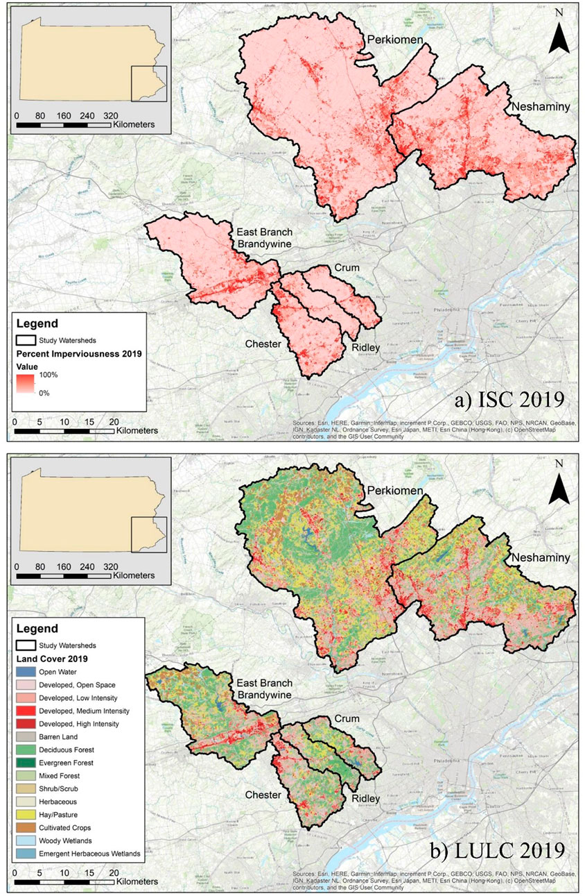
FIGURE 1. Maps of the six southeastern Pennsylvania watersheds and their underlying impervious surface cover (ISC) and land use land cover (LULC); (A) ISC from 2019 and (B) LULC from 2019.

2.2 Major ions and discharge data

Streamwater quality data for major cations (Na⁺, K⁺, Mg²⁺, Ca²⁺) and anions (Cl⁻, SO₄^2-, and HCO₃⁻), including concentrations, were obtained from Aqua Pennsylvania, Inc (Aqua), a regional water utility for the years 1999–2019. Of note, HCO₃⁻ concentrations were calculated using the alkalinity (reported as CaCO₃). Water samples were obtained monthly from the streamwater tap located within the water utility plant in each of the study watersheds. Major ion concentrations were determined using ion chromatography, while the alkalinity as CaCO₃ concentrations were determined using titration. Daily mean discharge data for each day of the study period were determined at the U.S. Geological Survey (USGS) gaging stations closest to the Aqua sampling sites (Supplementary Table S2), and downloaded from USGS Water Data for the Nation (U.S. Geological Survey, 2020). Except for Crum and Perkiomen, the gaging stations were located within approximately two miles of the respective sampling location.

2.3 Specific conductance calculations

The reported concentrations of dissolved constituents were used to compute the total dissolved solids (TDS), specific conductance at 25°C (SC), and ionic contributions to SC according to methods reported by Cravotta and Brady (2015) and McCleskey et al. (2023). The TDS was computed as the sum of major dissolved constituents, where the mass of the inorganic carbon in the residue is approximately half that in the original water sample and which approximates the mass in the anhydrous residue determined by the standard “residue on evaporation” measurement (U.S. Geological Survey, 1989). Aqueous speciation with PHREEQC (Parkhurst and Appelo, 2013) was used to determine the molal concentrations of aqueous species in order to compute the ionic contributions to SC, and the corresponding SC on the basis of those ions (McCleskey et al., 2012; McCleskey et al., 2023). The measured SC, which was available for the last 10 years of sampling, compared favorably to computed values of SC, as shown in Supplementary Figure S1.

2.4 Weighted regressions on time, discharge, and season analysis

Following the WRTDS methodology outlined in Rossi et al. (2022), the monthly streamwater quality parameters collected by Aqua along with the USGS daily mean discharge data for all days of the year were entered into the Weighted Regressions on Time, Discharge, and Season (WRTDS) model within the Exploration and Graphics for RivEr Trends (EGRET) program in R (Hirsch and De Cicco, 2015; Hirsch et al., 2018a). The model was used to calculate the average annual flow-normalized concentrations for Na⁺, Mg²⁺, Ca²⁺, Cl⁻, SO₄^2-, and HCO₃⁻, in all six watersheds. K⁺ was calculated for Chester, Neshaminy, and Perkiomen watersheds only, due to a lack of data. The average annual flow-normalized concentrations for each water quality parameter were calculated for the water year (October-September) for 21 years of data. Likewise, they were calculated for baseflow months (August ̶ November; as determined by an analysis of long-term monthly flow data for the study watersheds), and winter months (December ̶ March). The flow normalization equation used in the WRTDS method can be defined as follows:

$E\left[C_{fn}\left(T\right)\right]={\displaystyle {\int }_0^{\infty }}w\left(Q,T\right)·f_{Ts}\left(Q\right)dQ$

Where $E\left[C_{fn}\left(T\right)\right]$ is the flow-normalized concentration for time T (a specific day of a specific year), $w\left(Q,T\right)$ is the WRTDS estimate of concentration as a function of Q (discharge) and T (time, years), and $f_{Ts}\left(Q\right)$ is the probability density function (pdf) of discharge, specific to a particular time of year, designated as Ts (Hirsch and De Cicco, 2015). The WRTDS model gives increased weight to data points that are similar in time, streamflow, and season, using a tricube weight function with a half-window width of 7 years in the time dimension, 2 natural log units in the streamflow dimension, and 0.5 years in the seasonal dimension (Corsi et al., 2015).

Similar to Rossi et al. (2022) and consistent with other recent studies, this study uses the extended methodology of the WRTDS model, which assumes the probability distribution of discharge is non-stationary from year to year, to calculate the management trend component (MTC) and streamflow trend component (QTC) (Choquette et al., 2019; Murphy and Sprague, 2019; Mazumder et al., 2021; Rossi et al., 2022). The MTC shows how watershed management (such as development) impacts trends, while the QTC shows how changes in streamflow impact trends. The sum of the MTC and QTC is the water quality trend (WQT). To run the extended WRTDS methodology, it is recommended that the change in discharge over the study period is greater than 10%. A streamflow trend analysis demonstrated that the changes in the median and mean daily discharge values were greater than 10% over the study period in all watersheds except Crum and Perkiomen.

The block-bootstrap technique was used to determine the uncertainty of the WQT for each water quality parameter (Na⁺, Mg²⁺, Ca²⁺, K⁺, Cl⁻, SO₄^2-, and HCO₃⁻) using the EGRETci package in R (Hirsch et al., 2018b). For each site, 100 bootstrap replicates were performed, and the likelihood that the trend direction was correct was computed (Murphy and Sprague, 2019). Although the same study watersheds and methods are utilized as those referenced in Rossi et al. (2022), this study builds upon the aforementioned study. Rossi et al. (2022) focuses on changes in Cl⁻ concentrations over time and its relationship with ISC and road salt. This study analyzes additional ions (Na⁺, Mg²⁺, Ca²⁺, SO₄^2-, and HCO₃⁻) to evaluate the FSS, and its relationship with controlling factors, such as WWTP discharge volume, % ISC and % agriculture in the upstream area. Additionally, these ions are used to calculate the CSMRs and LRs and evaluate potential impacts to drinking water infrastructure.

2.5 Chloride to Sulfate Mass Ratio and Larson Ratio

Annual CSMR and LR values were calculated for each year of the study period to determine the relative change over time for potential corrosivity of surface water. The CSMR has been previously used to describe the potential for water to corrode lead and iron infrastructure (Nguyen et al., 2011; Pieper et al., 2017; Stets et al., 2018). We calculated the CSMR using the annual flow-normalized chloride and sulfate concentration values from the WRTDS model as follows:

$\mathrm{C}\mathrm{S}\mathrm{M}\mathrm{R}={\mathrm{C}\mathrm{l}}^{-}/{\mathrm{S}\mathrm{O}}_4^{2-}(1)$

where the Cl⁻ concentration (mg L^-1) is divided by SO₄^2- (mg L^-1). A non-flow-normalized CSMR value greater than ∼0.5 can accelerate corrosion of metallic components in drinking water facilities and distribution networks (Edwards and Triantafyllidou, 2007; Nguyen et al., 2011; Pieper et al., 2017).

Additionally, the Larson Ratio describes the potential for water to corrode iron and steel pipes, but combines Cl⁻ and SO₄⁻ and also takes alkalinity into account (Larson and Skold, 1958; Stets et al., 2018). We calculated the LR using the annual flow-normalized chloride, sulfate, and alkalinity concentration values from the WRTDS model as follows:

$\mathrm{L}\mathrm{R}=\left(\left({\mathrm{C}\mathrm{l}}^{-}/35.453\right)+\left(2\mathrm{x}\left({\mathrm{S}\mathrm{O}}_4^{2-}/96.06\right)\right)\right)/\left(\left(\mathrm{A}\mathrm{l}\mathrm{k}\mathrm{a}\mathrm{l}\mathrm{i}\mathrm{n}\mathrm{i}\mathrm{t}\mathrm{y}/50.04\right)\right)(2)$

where Cl⁻ (mg L^-1), SO₄^2- (mg L^-1), and alkalinity (mg L^-1 as CaCO₃) concentrations were divided by their respective molecular mass and multiplied by their associated valence charge to convert to equivalents. A non-flow-normalized LR value greater than 1.2 indicates a greater potential for corrosion than lower values (Agatemor and Okolo, 2008; Masten et al., 2016).

2.6 Impervious surface cover and land use land cover analysis

The watersheds were delineated as described in Rossi et al. (2022) using ArcMap 10.8.1 and ArcHydro (ESRI, Inc., Redlands, CA). Additionally, the total percentages of impervious surface cover (ISC) and land use land cover (LULC) classes for the years 2001, 2004, 2006, 2008, 2011, 2013, 2016, and 2019 were determined for each watershed as described in Rossi et al. (2022), using data obtained from the National Land Cover Database (NLCD) on the Multi-Resolution Land Characteristics Consortium website (Yang et al., 2018; Jin et al., 2019; Homer et al., 2020; Multi-Resolution Land Characteristics Consortium, 2021a; Multi-Resolution Land Characteristics Consortium, 2021b). The calculated percent change of LULC and imperviousness is the percentage value in 2001 subtracted from the percentage value in 2019. Supplementary Table S3 describes the NLCD LULC classes that were combined to create the three LULC categories used in this analysis (developed, agricultural, and forested land).

2.7 National pollutant discharge elimination system (NPDES) permits

NPDES permits issued for all sewage treatment plants (STPs) and non-industrial wastewater treatment plants (WWTPs) within the study watersheds were compiled using the USEPA’s Facility Registry Service dataset (Environmental Protection Agency Facility Registry Service, 2021). The permit number and total permitted discharge volume were documented for each STP and non-industrial WWTP. We cross-referenced our permit search by using the historical imagery feature in Google Earth to determine if the STPs and WWTPs were active for the entire study period and adjusted the permitted discharge volume accordingly.

2.8 Statistical analyses

Most statistical analyses presented herein were carried out using R software Version 4.0.4 (R Core Team, 2021) and JMP 16.0.0 (2022). Pearson correlation analysis between the change in annual WQT/baseflow MTC values and the absolute change in percent ISC, agriculture, and forest cover was performed using the statistical software JMP (JMP, 2022). A redundancy analysis (RDA) was conducted using the “vegan” package in R to evaluate the influence of ion sources (i.e., ISC, agricultural land use, and WWTP effluent) on stream chemistry data for the years 2001 and 2019, using the annual WQT and baseflow (August-November) MTC values (Okansen et al., 2020). An RDA is the direct extension of multiple regression to model multivariate response data while constraining the ordination of dependent variables to linear combinations of independent variables (Legendre and Legendre, 2012; Li et al., 2018; Tanaka et al., 2016). An RDA generates a two-dimensional chart which visualizes the relationship of the dependent variables (points in the graph) with the independent variables (vectors) (Tanaka et al., 2016). For our RDA, %ISC, %agricultural land use as well as total WWTP effluent in the upstream area were selected as independent variables given the wealth of literature describing their influence on major ion chemistry in mixed use watersheds. Prior to analysis all variables were checked for normality. The significance of the RDA models was verified using a Monte Carlo permutation test (719 permutations) (Tanaka et al., 2016).

3 Results

As indicated by the long-term positive linear trends in SC (Figure 2) and nearly identical patterns for TDS, salinization is clearly occurring in all six watersheds. Because the SC, TDS, and, therefore, the FSS are the result of variable ionic contributions, we examined the influence of changes in those individual ionic constituents and the factors affecting those changes.

FIGURE 2

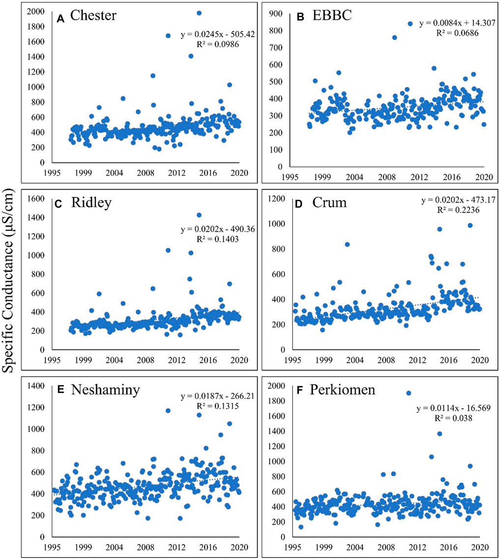
FIGURE 2. Calculated specific conductance over time in the following six watersheds: (A) Chester; (B) EBBC; (C) Ridley; (D) Crum; (E) Neshaminy; (F) Perkiomen. Specific conductance is increasing in each watershed, ranging from an increase of approximately 0.8%–2.5% per year. EBBC refers to the East Branch of Brandywine Creek watershed.

3.1 WRTDS model outputs

The MTC shows how watershed management (such as development) impacts trends, while the QTC shows how changes in streamflow impacts trends. The sum of the MTC and QTC is the water quality trend (WQT). The results for each ion are described in detail in Tables 1 and 2, and general trends are summarized below.

TABLE 1

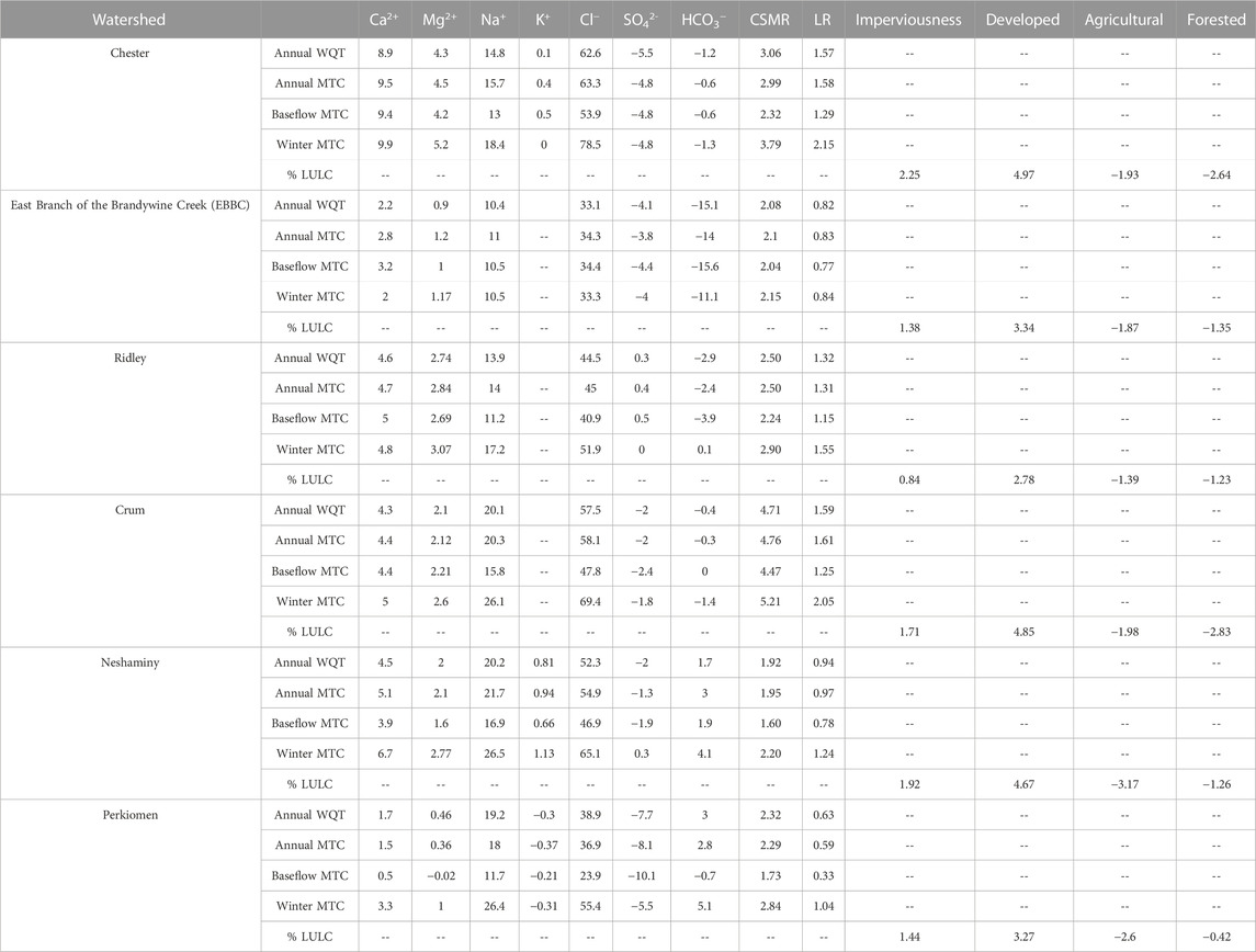
TABLE 1. The absolute change in various water quality parameters from 1999 to 2019 and imperviousness and land use land cover from 2001 to 2019. The absolute change in the annual water quality trend (WQT), management trend component (MTC), baseflow MTC, and winter MTC are calculated for Ca²⁺, Mg²⁺, Na⁺, K⁺, Cl⁻, SO₄^2-, HCO₃⁻, chloride to sulfate mass ratio (CSMR), and Larson Ratio (LR). EBBC refers to the East Branch of Brandywine Creek watershed.

TABLE 2

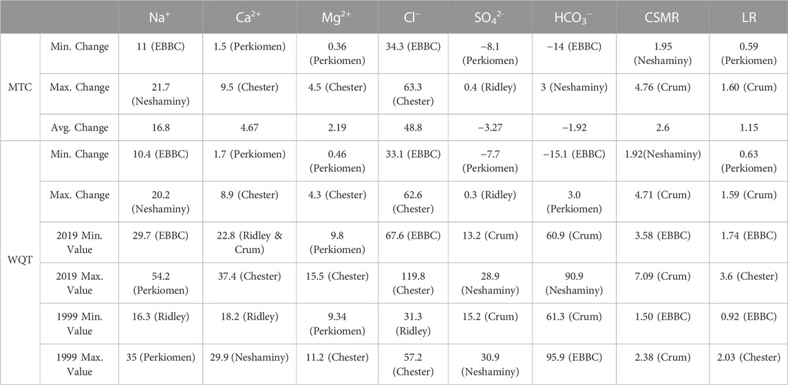
TABLE 2. Weighted Regressions on Time, Discharge, and Season (WRTDS) model output results for each ion (except K⁺). The table shows the minimum, maximum, and average changes in concentration (in mg L^-1) for the MTC (management trend component) and the WQT (water quality trend). The minimum and maximum concentrations in 1999 and 2019 (in mg L^-1) and the corresponding watershed are shown. EBBC refers to the East Branch of Brandywine Creek watershed.

The management trend component (MTC) for Na⁺, Ca²⁺, Mg²⁺, and Cl⁻ increased in all six watersheds over the study period, and there were minor changes in the QTC for these constituents (Table 2; Supplementary Tables S4–S6, S8; Figure 3). The overall flow-normalized water-quality trend, WQT (MTC + QTC), for Na⁺, Ca²⁺, Mg²⁺, and Cl⁻, increased in all six watersheds and the increasing trends were all likely or highly likely (Figures 3, 4A–C; Tables 1, 2; Supplementary Tables S4–S6, S8). For Na⁺, the percent change in the WQT ranged from 48.8% (Chester) to 119% (Crum), with an average of 70.6%. For Ca²⁺, the percent change in the WQT ranged from 6.18% (Perkiomen) to 31.2% (Chester), with an average of 18.1%. For Mg²⁺, the percent change in the WQT ranged from 4.93% (Perkiomen) to 38.4% (Chester), with an average of 20.0%. For Cl⁻, the percent change in the WQT ranged from 69% (Perkiomen) to 159% (Crum), with an average of 112.5%. Additionally, the 2019 winter MTC concentrations for Na⁺ and Cl⁻ were greater than the annual WQT, annual MTC, and baseflow MTC in all six watersheds, while the 2019 baseflow MTC concentrations for Na⁺ and Cl⁻ were lower than the annual WQT, annual MTC, and baseflow MTC in all six watersheds.

FIGURE 3

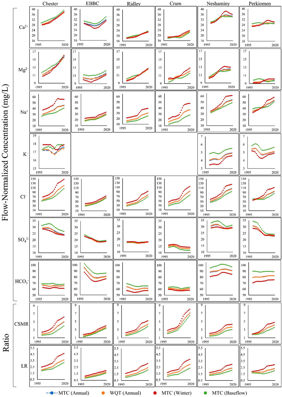
FIGURE 3. The management trend component (MTC; blue) and the water quality trend (WQT; sum of the management trend component and the streamflow trend component; orange) over the study period (1999–2019) in each of the six watersheds for the following water quality parameters: Ca²⁺, Mg²⁺, Na⁺, K⁺, Cl⁻, SO₄^2-, HCO₃⁻, CSMR (Chloride to Sulfate Mass Ratio), and LR (Larson Ratio). The MTC during baseflow months (August-November; green) and winter months (December-March; red) for each of the six watersheds is also shown. Please note, the y-axis scaling is the same for each ion, except for potassium. In the cases where you cannot see the Annual MTC trend, it is because it is behind the Annual WQT trend. EBBC refers to the East Branch of Brandywine Creek watershed.

FIGURE 4

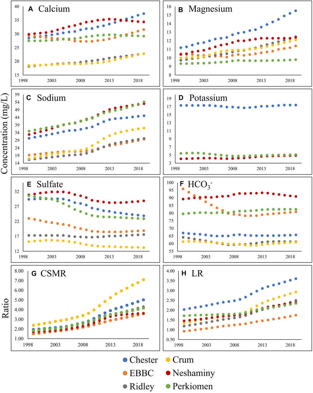
FIGURE 4. Change in annual flow-normalized concentration (water quality trend; in mg L⁻¹) over the study period (1999–2019 in Chester (blue), East Branch of the Brandywine Creek (EBBC; orange), Ridley (grey), Crum (yellow), Neshaminy (red), and Perkiomen (green)) for the following: (A) calcium; (B) magnesium; (C) sodium; (D) potassium; (E) sulfate; (F) bicarbonate; (G) CSMR (Chloride to Sulfate Mass Ratio); and (H) LR (Larson Ratio).

The overall flow-normalized K⁺ water-quality trend, WQT (MTC + QTC), remained relatively stable over the study period in Chester and Perkiomen (0.1 mg L^-1 and -0.3 mg L^-1, respectively) and increased slightly in Neshaminy watershed (0.81 mg L^-1) (Table 1; Supplementary Table S7; Figure 3, 4D). The stable trends were about as likely as not, while the increasing trend was highly likely. The percent change in the WQT for K⁺ over the study period ranged from −5.54% (Perkiomen) to 19.9% (Neshaminy), with an average of 4.98% (Supplementary Table S7).

The flow-normalized MTC and WQT for SO₄^2- decreased in five of the six watersheds over the study period, and the downward trend was highly likely (Tables 1, 2; Supplementary Table S9; Figures 3, 4E). The flow-normalized MTC and WQT for SO₄^2- remained relatively stable in Ridley watershed, and the trend was about as likely as not. In each watershed, the absolute change in the QTC was less than the absolute change in the MTC. The percent change in the WQT for SO₄^2- over the study period ranged from −25.2% (Perkiomen) to 1.73% (Ridley), with an average of −13.3% (Supplementary Table S9).

The flow-normalized MTC and WQT for HCO₃⁻ decreased in three of the six watersheds, increased in two others (Neshaminy and Perkiomen), and remained relatively stable in one watershed (Crum) over the study period (Tables 1, 2; Supplementary Table S10; Figure 3, 4F). The decreasing trends were highly likely, likely, and about as likely as not, while the increasing trends were likely and very likely. In five of the six watersheds, the absolute change in the QTC was less than the absolute change in the MTC. The percent change in the WQT for HCO₃⁻ over the study period ranged from −15.8% (EBBC) to 3.77% (Perkiomen), with an average of −2.85%. Additionally, the 2019 baseflow MTC concentrations were greater than the annual WQT, annual MTC, and winter MTC for all six watersheds, while the 2019 winter MTC concentrations were lower than the annual WQT, annual MTC, and winter MTC for all six watersheds.

The calculated MTC and WQT for both CSMR and LR increased in all six watersheds over the study period (Tables 1, 2; Supplementary Tables S11, S12; Figures 3, 4G, H). The percent change in the CSMR WQT over the study period ranged from 113% (Neshaminy) to 198% (Crum), with an average of 145%. The percent change in the LR WQT over the study period ranged from 36.8% (Perkiomen) to 120% (Crum), with an average of 83.3%. The 2019 winter MTC CSMR and LR values were greater than the annual WQT, annual MTC, and baseflow MTC for all six watersheds, while the 2019 baseflow MTC CSMR and LR values were lower than the annual WQT, annual MTC, and winter MTC for all six watersheds.

3.2 Sodium to chloride molar ratio

The sodium to chloride molar ratio (Na:Cl) significantly decreased in each of the six watersheds over the study period (Figure 5; Supplementary Table S13). The ratio is decreasing at the greatest rate in Chester, Neshaminy, and EBBC watersheds, with linear slope values of −0.0132, −0.0112, and −0.0101, respectively. In Chester, Neshaminy, and EBBC watersheds, Na:Cl remained relatively stable until 2004, after which the ratio started to decrease. In 1999, Neshaminy had the greatest Na:Cl of 0.965, while Crum had the smallest Na:Cl of 0.722 (Figure 5). In 2019, Perkiomen had the greatest Na:Cl of 0.877, while Chester had the smallest Na:Cl of 0.581 (Figure 5).

FIGURE 5

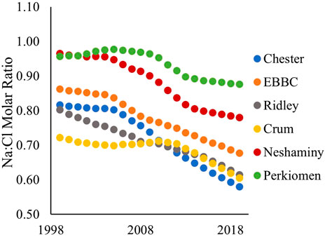
FIGURE 5. Sodium to chloride (Na:Cl) molar ratio in each of the six watersheds over the study period (1999–2019). EBBC refers to the East Branch of Brandywine Creek watershed.

3.3 Exceedances of water quality guidelines for Na⁺

Annual WQT, winter MTC, and baseflow MTC Na⁺ concentrations substantially increased in all six watersheds (>48.8, 46.3% and 29.6%, respectively). The 2019 annual WQT and baseflow MTC values for all watersheds exceeded the USEPA recommended threshold of 20 mg L^-1 for those on a low sodium diet (United States Environmental Protection Agency, 2003). The 2019 winter MTC values were greater than both the 2019 annual WQT and baseflow MTC values for all six watersheds.

Individual water samples exhibited spikes in Na⁺ concentrations (Table 3). For example, >90% of the water samples collected from Chester, Neshaminy, and Perkiomen watersheds exceeded the USEPA 20 mg L^-1 threshold, and anywhere from 2.28% to 11.4% of the samples from each watershed exceed the USEPA guidelines of 30–60 mg L^-1 for salty taste (Table 3). Additionally, all watersheds had at least one Na⁺ concentration in excess of 100 mg L^-1 while four (Chester, Ridley, Neshaminy and Perkiomen) had individual values in excess of 200 mg L^-1.

TABLE 3

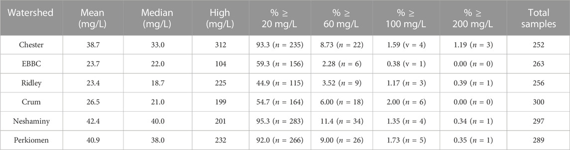
TABLE 3. Mean, median, and high sodium concentrations (in mg L^-1) for individual water samples collected from each watershed, as well as the percentage of samples that are greater than 20, 60, 100, and 200 mg L^-1. EBBC refers to the East Branch of Brandywine Creek watershed.

3.4 Land use land cover and impervious surface cover

As described in Rossi et al. (2022), ISC increased in each of the six watersheds from 2001 to 2019 (Figure 1A). The increase in ISC ranged from 0.84% (Ridley) to 2.25% (Chester), with an average increase of 1.59%. In 2019, total percent ISC ranged from 6.77% (Ridley) to 14.2% (Neshaminy). Similarly, developed land (combination of developed open space, low, medium, and high intensity categories) increased in each of the six watersheds, ranging from an increase of 2.78% (Ridley) to 4.97% (Chester) (Figure 1B). In 2019, total percent developed land ranged from 32.3% (Perkiomen) to 57.9% (Chester). Agricultural (combination of cultivated crops and hay/pasture categories) and forested land (combination of deciduous, evergreen, and mixed forest categories) decreased from 2001 to 2019. The decrease in agricultural land ranged from −1.39% (Ridley) to −3.17% (Neshaminy), while the decrease in forested land ranged from −0.42% (Perkiomen) to −2.83% (Crum). In 2019, agricultural land ranged from 9.11% (Chester) to 28.5% (Perkiomen), while forested land ranged from 21.2% (Neshaminy) to 39.6% (Ridley).

3.5 Relationship between WQT/MTC solute concentrations, ISC, LULC, and WWTP discharge volume

To evaluate the influence of ISC, agricultural land use, and WWTP effluent on stream chemistry, an RDA was conducted using annual WQT and baseflow (August ̶ November) MTC values for the six watersheds in 2001 and 2019 (Table 4). The baseflow RDA should elucidate the influence of FSS on shallow groundwater and potential effects from subsurface ion exchange on streamwater solute concentrations.

TABLE 4

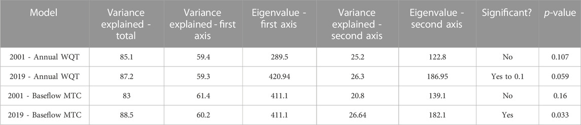
TABLE 4. Numerical model outputs from the four RDA models.

3.5.1 RDA with annual WQT values

The RDA models for 2001 and 2019 indicated relations of major ions to ISC, WWTP, and agriculture, but with changes to relative importance of those factors. Though the 2001 model relationship between stream chemistry and watershed land use was not significant (p = 0.107), the RDA using annual WQT values showed that Cl⁻, and Mg²⁺ were proximally associated with sites dominated by ISC, Na⁺ and SO₄^2- were proximally associated with sites dominated by ISC and WWTP discharge volume, Ca²⁺ was proximally associated with sites dominated by WWTP discharge volume, and HCO₃⁻ was proximally associated with sites dominated by agriculture (Figure 6A).

FIGURE 6

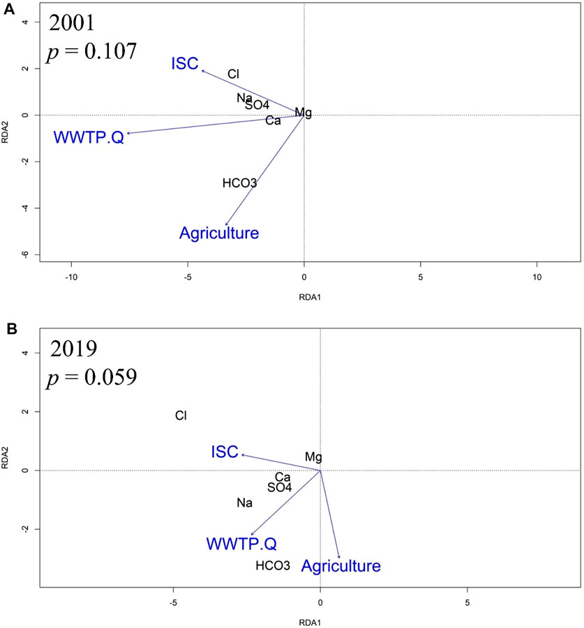
FIGURE 6. RDA showing a biplot of relations among the stream chemistry WQT (water quality trend) values, percentages of impervious surface cover (ISC) and agricultural land, as well as WWTP discharge volume (WWTP.Q) in (A) 2001 and (B) 2019.

The 2019 RDA model demonstrated that the relationship between stream chemistry and watershed land use was significant for 0.1 but not 0.05 (p = 0.059). Cl⁻, Mg²⁺ and Ca²⁺ were proximally associated with sites dominated by ISC, Na⁺ and SO₄^2- were proximally associated with sites dominated by ISC and WWTP discharge volume, and HCO₃⁻ was proximally associated with sites dominated by agriculture and WWTP discharge volume (Figure 6B).

3.5.2 RDA with annual average baseflow (August ̶ November) MTC values

As with the 2001 annual WQT RDA, the 2001 baseflow model relationship between stream chemistry and watershed land use was not significant (p = 0.16) and showed that Cl⁻, and Mg²⁺ were proximally associated with sites dominated by ISC, Na⁺ and SO₄^2- were proximally associated with sites dominated by ISC and WWTP discharge volume, Ca²⁺ was proximally associated with sites dominated by WWTP discharge volume, and HCO₃⁻ was proximally associated with sites dominated by agriculture (Figure 7A).

FIGURE 7

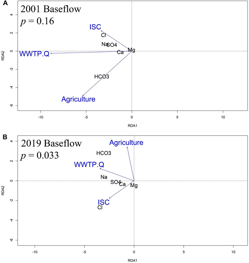
FIGURE 7. RDA analysis showing a biplot of relations among the stream chemistry baseflow (August–November) MTC values, percentages of impervious surface cover (ISC) and agricultural land, as well as WWTP discharge volume (WWTP.Q) in (A) 2001 and (B) 2019.

For the 2019 baseflow MTC model, the relationship between stream chemistry and watershed land use was significant (p = 0.033), and as with the 2019 annual WQT analysis, the 2019 baseflow MTC RDA showed that Cl⁻, Mg²⁺ and Ca²⁺ were proximally associated with sites dominated by ISC, SO₄^2- was proximally associated with sites dominated by ISC and WWTP discharge volume, Na⁺ was proximally associated with sites dominated by WWTP discharge volume, and HCO₃⁻ was proximally associated with sites dominated by agriculture and WWTP discharge volume (Figure 7B).

4 Discussion

4.1 Evidence for the FSS in suburban and exurban watersheds

To identify if the FSS is occurring in the study watersheds, we first evaluated the influence of natural geologic sources on solutes. For example, annual flow-normalized (WQT) values for Na⁺ (16.3 ̶ 54.2 mg L^-1) and Cl⁻ (31.3 ̶ 120 mg L^-1) in this study are well above background values for regional streams and groundwater (8 and 10 mg L^-1, respectively; Biesecker et al., 1968). WQT values for Ca²⁺ (18.2–37.4 mg L^-1), Mg²⁺ (9.34–15.5 mg L^-1), and HCO₃⁻ (61.3 ̶ 90.9 mg L^-1) are relatively closer to background (<5, 8, and 60 mg L^-1, respectively; Biesecker et al., 1968), though elevated nonetheless. Therefore, the observed changes in concentrations over decadal timeframe reflect the cumulative influx of salt, disturbance in mineral weathering rates, and/or stability of constructed materials. Substantial increases in annual WQT for Na⁺, Ca²⁺, Mg²⁺, and Cl⁻ were observed in all six study watersheds (ranging from 4.9% to 159%). Furthermore, increases in MTC were observed for those constituents during winter (December–March), which is a higher flow period due to a greater fraction of runoff, and also during summer/fall (August-November), which is baseflow dominated by groundwater, with the exception of baseflow Ca²⁺ and Mg²⁺ in Perkiomen watershed. A relative lack of increase in Ca²⁺ and Mg²⁺ baseflow MTC values in Perkiomen watershed could be attributed to it being with largest watershed in size while having the second lowest amount of ISC. Previous studies evaluating facets of the FSS have identified similar trends in road salt affected regions (Bird et al., 2018; Kaushal et al., 2018). This co-relationship of solutes was further supported by a strong positive statistical relationship between changes in annual WQT values for Ca²⁺, Mg²⁺, and Cl⁻ (R_avg = 0.87, p < 0.05). Furthermore, the strength of correlation between these parameters increased when comparing the changes in baseflow MTC values (R_avg = 0.90, p < 0.03), suggestive of groundwater impacts and influence.

The dominant form of road salt applied to roads in this study was NaCl. Nevertheless, the molar ratio of Na:Cl in streamwater samples was <1.0 (Figure 5). Although the MTC of Cl⁻ and Na⁺ increased over the decadal timeframe, the MTC of Cl⁻ increased at a faster rate than that of Na⁺, which resulted in decreasing Na:Cl with increasing time. Decreases in Na:Cl have also been observed in other non-urban watersheds (Dailey et al., 2014; Bird et al., 2018). The observed Na:Cl < 1.0 is consistent with reverse cation exchange and the cumulative build-up of Na⁺ in soils while Cl⁻ and displaced cations (Ca²⁺, Mg²⁺, and K⁺) are exported, as has also been observed in coastal areas undergoing salinization (Martínez and Bocanegra, 2002; Askri et al., 2022). Because cation exchange mainly affects groundwater, the decreasing Na:Cl with time may be explained by a lag in the discharge of groundwater to the stream, which consists of groundwater (baseflow) and runoff in relatively constant proportions on an annual basis. More recently recharged groundwater, which has been influenced by greater salt loading, has greater Na and Cl concentrations and a lower Na:Cl ratio than older groundwater. With progressively increased time, the fraction of older groundwater, less influenced by salt loading, decreases while that recharged more recently increases in the baseflow.

An RDA identified present day relationships between road salt affected solutes and either ISC or development in the upstream areas. For example, the WQT sourced RDA showed a present-day (2019) statistical association between percent ISC and Cl⁻, Mg²⁺, and Ca²⁺ concentrations (Figure 6). Interestingly, the statistical significance of the RDA model improved when only considering baseflow MTC values (p = 0.059 vs. p = 0.033; Figure 7), further supporting a watershed-scale effect on shallow groundwater and a subsurface mechanism for ion interactions. Additionally, the statistical significance of the WQT and MTC sourced RDA models strengthened from 2001 to 2019. The WQT-sourced RDA showed a significant association between Na⁺ concentration, ISC, and total WWTP discharge volume in the upstream area, while the MTC-sourced baseflow RDA showed a strong association between Na⁺ concentration and WWTP discharge volume, only. The former is likely attributed to increased Na⁺ inputs from stormwater runoff from impervious surfaces during snowmelt events (Interlandi and Crockett, 2003; Kelly et al., 2012; Dailey et al., 2014; Moore et al., 2017), while the latter is due to WWTPs being a substantial source of Na⁺ during baseflow conditions (Kaushal et al., 2005; Steele and Aitkenhead-Peterson, 2011). For example, human waste, detergents, and disinfectants are notable sources of Na⁺ which is not affected by wastewater treatment (Metcalf et al., 1991; Kelly et al., 2008). Additionally, sodium hypochlorite (aka chlorine bleach) can be added to wash water and wastewater to reduce the presence of harmful microorganisms (Veschetti et al., 2003).

Relationships were observed between road salt related and displaced ions, percent ISC, and development in upstream areas. We found a positive relationship between the absolute change in WQT Cl⁻ concentrations from 2001 to 2019 and the change in percent ISC within the upstream area (r = 0.71, p = 0.12) and a negative weakly significant relationship between the absolute change in WQT Cl⁻ concentrations and the change in percent forested land in the upstream area (r = −0.79, p = 0.06). Additionally, a positive weakly significant relationship was observed between the absolute change in the baseflow MTC Na⁺ concentration and the change in percent developed open space (r = 0.76, p = 0.08), while a positive significant relationship was observed between the absolute change in the baseflow MTC Na⁺ concentration and the change in low-density development in the upstream area (r = 0.82, p = 0.05). Interlandi and Crockett (2003) identified a similar increase in Na⁺ and Cl⁻ concentrations coupled with an increase in total developed land and a decrease in forested land in the nearby Schuylkill River watershed. Mazumder et al. (2021) also identified an increase in Cl⁻ concentrations coupled with increased development in the Toronto, Canada metropolitan region. Additionally, we found a positive, yet non statistically significant relationship between the absolute change in Ca²⁺ and Mg²⁺ concentrations and the absolute change in percent ISC, and a negative and weakly significant relationship with the change in percent forest cover. This further suggests that increased road salt use and increased development and percent ISC lead to the mobilization of cations. In the closest study to our own methodologically, Bird et al. (2018) found an increase of Na⁺, Ca²⁺, Mg²⁺, and Cl⁻ concentrations in road salt-affected watersheds in the mid-Atlantic region of the U.S., with greater increases observed in watersheds with higher percent ISC. However, their study observed steady state development in the same watersheds. Collectively, these findings suggest that while overland flow and WWTP effluent can influence the delivery for some base cations (e.g., sodium) in mixed use watersheds, subsurface ion exchange and baseflow inputs play the predominant role for the others. Additionally, increased %ISC and development in the upstream area over time, and consequent road salt application, appears to be the driving force behind this change.

4.2 Other solutes

Sulfate decreased in five of the six watersheds over the study period. These decreasing SO₄^2- concentrations are likely the result of a decrease in atmospheric deposition and flushing of the accumulated SO₄^2- from watersheds over past decades due to more stringent air pollution policies, such as the Acid Rain Program, an amendment to the Clean Air Act (National Atmospheric Deposition Program, 1997; Elkin et al., 2016; Bird et al., 2018; Stets et al., 2018; National Atmospheric Deposition Program, 2020; United States Environmental Protection Agency, 2022a). Other studies in the mid-Atlantic and northeastern U.S. have found similar decreases in SO₄^2- concentrations over time in streamwater (Moore et al., 2017; Bird et al., 2018). Though a general decreasing trend was observed, there were nuances in the data. For example, Chester and Neshaminy, which had the greatest percentages of ISC, also had the greatest SO₄^2- concentrations at the end of the study period. These elevated concentrations could be partially attributed to weathering of gypsum in concrete (Lerch, 2008; Lothenbach et al., 2008) and to additional inputs from surfactants (detergents and shampoos) and WWTP process chemicals (Metcalf et al., 1991). Perkiomen, which is the largest watershed and is composed of the greatest percentage of agricultural land, had the third highest SO₄^2- concentrations over the study period. Given this watershed is less developed, with just 8.23% of ISC (Rossi et al., 2022), the elevated SO₄^2- concentration could be a result of fertilizer (ammonium sulfate) and gypsum applications to agricultural fields (Schilling and Wolter, 2001; Spoelstra et al., 2021). Additionally, Perkiomen watershed has the second largest WWTP inputs, indicating that the elevated SO₄^2- concentrations could also be from detergents and WWTP process chemicals (Metcalf et al., 1991).

The WQT for HCO₃⁻ decreased by ∼16% in EBBC, slightly decreased (<5%) in Chester, Crum, and Ridley, and slightly increased in Neshaminy and Perkiomen. Interestingly, the Neshaminy and Perkiomen watersheds also had the highest amount of permitted WWTP discharge. While carbonate bedrock underlies some of parts of several watersheds, we found no relationship between spatial extent of the bedrock and current WQT HCO₃⁻ concentrations (R² = 0.09, p = 0.57), in contrast with a previous study for the region (Kaushal et al., 2013). Additionally, we did not observe an inverse relationship between HCO₃⁻ and SO₄⁻² concentrations, which might be expected if decreased acid deposition resulted in greater residual alkalinity (Likens et al., 1996; Kaushal et al., 2017). Thus, HCO₃⁻ trends appear to be driven by land use or WWTP discharge trends. For example, EBBC exhibited a large decrease in WQT/MTC values for HCO₃⁻ between 2001 ̶ 2010, which coincides with the timing of the greatest decrease in agricultural land. After 2010, the HCO₃⁻ concentration levels out and slightly increases in this watershed, which coincides with a stabilization of percent agricultural land and a modest increase in percent ISC.

Previous studies have found liming of agricultural fields to be a substantial source of HCO₃⁻ to waterways (Raymond et al., 2008; Barnes and Raymond, 2009; Kaushal et al., 2018). Thus, a decrease in percent agricultural land could conceivably account for decreases in HCO₃⁻. Conversely, weathering of concrete and increased sewage discharge coupled with population growth has been shown to increase HCO₃⁻ concentrations in urbanizing watersheds (Daniel et al., 2002; Barnes and Raymond, 2009; Kaushal et al., 2013). Regardless, the influence of land use and wastewater is supported by our RDA analysis, which found HCO₃⁻ concentrations to be causally related to both the percent agricultural land and total WWTP discharge volume in the upstream areas. Though a slight proximal shift of HCO₃⁻ towards the agricultural axis for the baseflow RDA suggests an important contribution from subsurface discharge.

4.3 Implications for sodium in drinking water

Substantial increases in annual WQT, winter MTC, and baseflow MTC Na⁺ concentrations were observed for all six watersheds (>48.8, 46.3, and 29.6%, respectively). However, winter concentrations were greater than both the annual WQT and the baseflow MTC concentrations over the study period. Furthermore, >90% of the water samples collected from Chester, Neshaminy, and Perkiomen watersheds exceeded the USEPA recommended threshold of 20 mg L^-1 for those on a low sodium diet (United States Environmental Protection Agency, 2003). Additionally, several individual samples exhibited Na⁺ concentrations well in excess of the USEPA guidelines of 30–60 mg L^-1 for salty taste. As previously mentioned, Chester, Neshaminy, and Crum experienced the greatest increases in percent ISC over the study period. Furthermore, Crum had the greatest percent increase of Na⁺ from 2008 to 2019 at ∼64% (Rossi et al., 2022). Previous studies have found increasing Na⁺ concentrations over time (Interlandi and Crockett, 2003; Dailey et al., 2014), and in the Baltimore region, studies have found that watersheds with greater ISC also exhibited greater Na⁺ concentrations (Moore et al., 2017; Bird et al., 2018).

All Na⁺ concentrations greater than or equal to 100 mg L^-1 occurred during winter and early spring months (Jan-March), except for one sample in October in Perkiomen watershed. Thus, spikes in Na⁺ concentrations are likely a result of road salt runoff. These results support a recent finding of short-term spikes of Na⁺ concentrations in Philadelphia tap water following snow melt events (Cruz et al., 2022). The two watersheds which exhibited the greatest Na⁺ concentrations in 2019 (Perkiomen and Neshaminy) flow into rivers which are ultimately drawn upon by the City of Philadelphia for municipal water supply (Schuylkill and Delaware River, respectively). Thus, corresponding changes in %ISC and WWTP effluent in the study watersheds are negatively influencing the quality of drinking water supply of downstream municipalities. Regardless, both average values and spikes in Na⁺ concentrations can result in individuals consuming greater than 30% of their daily recommended Na⁺ input through drinking water; this is especially harmful to those following a low Na⁺ diet due to a predisposed risk of hypertension (Hallenbeck et al., 1981; Tuthill and Calabrese, 1981; Talukder et al., 2017; Cruz et al., 2022).

4.4 Implications for drinking water infrastructure and treatment

Two different methods of corrosivity were calculated, the CSMR and LR, which both indicated corrosive conditions with increasing severity over a decadal time scale. Each ratio was calculated using the reported data and the flow-adjusted WQT concentrations, which yielded equivalent values and therefore, comparable exceedances of relevant corrosivity thresholds. The WQT CSMR increased by a minimum factor of 2.13 in all six watersheds throughout the study period. In 2019, the WQT CSMR was greater than 3.58 in all watersheds, exceeding the 0.5 threshold, which is considered a risk for increasing corrosivity in drinking water supply networks, by a factor of 7.2 (Nguyen et al., 2011; Masten et al., 2016; Pieper et al., 2017). Crum watershed exhibited a CSMR value that exceeded the threshold by a factor of 14. Interestingly, the 2019 median WQT CSMR value was slightly greater than that previously identified for watersheds throughout the U.S. with similar percentages of developed and agricultural land (Stets et al., 2018); though all watersheds were impacted by road salt application. The highest rates of increase in CSMR values were observed in watersheds with the greatest increases in %ISC, a finding previously identified by Rossi et al. (2022). Additionally, the positive correlation between the change in WQT CSMR values with the absolute change in percent developed open space along with the negative correlation with the absolute change in percent forest cover further suggests changes in development and road salt use are driving changes in CSMR values. Though decreasing SO₄^2- concentrations over the study period affect CSMR values, the percent change in the SO₄^2- WQT concentrations (−25.2%–1.73%) is much smaller than the percent change in the Cl⁻ WQT concentrations (69%–159%). Thus, changes in development and widespread road salt use are largely driving the increase in the CSMR over the study period.

The WQT LR increased by a minimum of 36% in all six watersheds throughout the study period. In 2019, the LR was greater than 1.74, exceeding the 1.2 threshold known for increasing corrosivity in drinking water supply networks by a factor of 1.5 (Agatemor and Okolo, 2008; Masten et al., 2016). Chester watershed exhibited an LR value that exceeded the threshold by a factor of 3. A statistically significant negative correlation was observed between the absolute change in the WQT LR values and the change in percent forested land in the upstream areas. Similar to the CSMR values, the median 2019 WQT LR value was slightly greater than that previously identified for watersheds throughout the U.S. with similar percentages of developed and agricultural land (Stets et al., 2018). Though the LR values are elevated, they are not as severe as the values for the CSMR because they take alkalinity into account. Therefore, Neshaminy and Perkiomen watersheds, both of which had slightly increasing WQT HCO₃⁻ concentrations over time, had the smallest percent changes in the LR over time at 64.8% and 36.8%, respectively. The absolute change in the WQT LR was also positively and significantly correlated with the absolute change in the WQT Mg²⁺, Ca²⁺, and Cl⁻ concentrations (R_avg = 0.82, p < 0.048); this correlation improves slightly when solely considering the baseflow MTC (R_avg = 0.88, p < 0.03). Thus, watersheds experiencing FSS-related increases in Cl⁻ export have higher LR values and a greater potential for corrosivity.

Public water suppliers apply corrosion inhibitors, such as orthophosphates (Volk et al., 2000; United States Environmental Protection Agency, 2016a), to prevent releases of lead and copper from water distribution networks into drinking water and the disintegration of the distribution pipe networks. However, increasing corrosivity ratios will likely result in increased costs to water utilities to mitigate the risks. This is especially true after snowfall and subsequent melting events when the Cl⁻ concentration in streamwater will be elevated and spike to extreme values due to road salt runoff (Interlandi and Crockett, 2003; Kaushal et al., 2005; Steele et al., 2010; Kelly et al., 2012; Corsi et al., 2015; Moore et al., 2017). Additionally, increased water corrosivity could translate to increased potential for drinking water main breaks, further increasing costs for water utilities.

5 Conclusion

The results of this study improve the understanding of the driving factors and cumulative impacts of road salting and the development of the freshwater salinization syndrome (FSS) in suburban and exurban watersheds. Increases in flow-normalized concentrations of Ca²⁺, Mg²⁺, Na⁺, and Cl⁻ that were observed in the six study watersheds, based on monthly sampling from 1999 to 2019 of streamwater at municipal intakes, demonstrate active FSS in areas undergoing development. The RDA results suggest road salt application is likely responsible for increased Ca²⁺ and Mg²⁺ concentrations, which we hypothesize is due to Na⁺ initiated reverse cation exchange in soils and subsequent export of displaced cations in groundwater to streams. In contrast, flow-normalized SO₄^2- concentrations decreased over time in five of the six watersheds. The decreases in SO₄^2- accentuate the effects of increasing Cl⁻ on corrosion potential, indicated by the CSMR. Both the CSMR and LR corrosivity indices increased over time in each of the six watersheds and presently (2019) exceed thresholds associated with corrosion of lead, iron, and steel pipes by as much as a factor of 14 and 3, respectively. From a human health perspective, annual average Na⁺ concentrations well exceed the USEPA recommended threshold for those following a low sodium diet (20 mg L^-1), with individual samples of streamwater greater than 10x this value. Generally, watersheds with the greatest percentages of ISC, also had the greatest percentages of samples that exceeded this threshold. Collectively, the study results demonstrate the importance of long-term monitoring of water chemistry and stream discharge in order to document and address water supply concerns and to mitigate impacts to human health and infrastructure.

Data availability statement

The original contributions presented in the study are included in the article/Supplementary Material, further inquiries can be directed to the corresponding author.

Author contributions

MR: conceptualization, data curation, formal analysis, funding acquisition, investigation, methodology, validation, supervision, visualization, writing–original draft, writing–review and editing. PK: formal analysis, writing–review and editing. CC: formal analysis, writing–review and editing. KS: data curation, writing–review and editing. SG: conceptualization, data curation, formal analysis, funding acquisition, investigation, methodology, supervision, validation, visualization, writing–original draft, writing–review and editing. All authors listed have made a substantial, direct, and intellectual contribution to the work and approved it for publication.

Acknowledgments

This study would not have been possible without the water quality data provided by Aqua Pennsylvania, Inc. Funding for the study was supplied by the College of Liberal Arts and Sciences at Villanova University. We thank helpful reviews by Andrew Reif and Blaine McCleskey of USGS and anonymous journal selected peers. Any use of trade, firm, or product names is for descriptive purposes only and does not imply endorsement by the U.S. Government.

Conflict of interest

KS was employed by the company Aqua Pennsylvania, Inc.

The remaining authors declare that the research was conducted in the absence of any commercial or financial relationships that could be construed as a potential conflict of interest.

Publisher’s note

All claims expressed in this article are solely those of the authors and do not necessarily represent those of their affiliated organizations, or those of the publisher, the editors and the reviewers. Any product that may be evaluated in this article, or claim that may be made by its manufacturer, is not guaranteed or endorsed by the publisher.

Supplementary material

The Supplementary Material for this article can be found online at: https://www.frontiersin.org/articles/10.3389/fenvs.2023.1153133/full#supplementary-material

References

Agatemor, C., and Okolo, P. O. (2008). Studies of corrosion tendency of drinking water in the distribution system at the University of Benin. Environmentalist 28 (4), 379–384. doi:10.1007/s10669-007-9152-2

CrossRef Full Text | Google Scholar

Aizer, A., Currie, J., Simon, P., and Vivier, P. (2018). Do low levels of blood lead reduce children’s future test scores? Am. Econ. J. Appl. Econ. 10 (1), 307–341. doi:10.1257/app.20160404

PubMed Abstract | CrossRef Full Text | Google Scholar

Askri, B., Ahmed, A. T., and Bouhlila, R. (2022). Origins and processes of groundwater salinisation in Barka coastal aquifer, Sultanate of Oman. Phys. Chem. Earth 126, 103116. doi:10.1016/j.pce.2022.103116

CrossRef Full Text | Google Scholar

Bäckström, M., Karlsson, S., Bäckman, L., Folkeson, L., and Lind, B. (2004). Mobilisation of heavy metals by deicing salts in a roadside environment. Water Res. 38 (3), 720–732. doi:10.1016/j.watres.2003.11.006

PubMed Abstract | CrossRef Full Text | Google Scholar

Barnes, R. T., and Raymond, P. A. (2009). The contribution of agricultural and urban activities to inorganic carbon fluxes within temperate watersheds. Chem. Geol. 266, 318–327. doi:10.1016/j.chemgeo.2009.06.018

CrossRef Full Text | Google Scholar

Biesecker, J. E., Lescinsky, J. B., and Wood, C. R. (1968). Water resources of the Schuylkill River basin. Pennsylvania Department of Forests and Waters Water Resources Bulletin, 198. No. 3.

Google Scholar

Bird, D. L., Groffman, P. M., Salice, C. J., and Moore, J. (2018). Steady-state land cover but non-steady-state major ion chemistry in urban streams. Environ. Sci. Technol. 52 (22), 13015–13026. doi:10.1021/acs.est.8b03587

PubMed Abstract | CrossRef Full Text | Google Scholar

Cecil, K. M., Brubaker, C. J., Adler, C. M., Dietrich, K. N., Altaye, M., Egelhoff, J. C., et al. (2008). Decreased brain volume in adults with childhood lead exposure. PLoS Med. 5 (5), e112. doi:10.1371/journal.pmed.0050112

PubMed Abstract | CrossRef Full Text | Google Scholar

Choquette, A. F., Hirsch, R. M., Murphy, J. C., Johnson, L. T., and Confesor, R. B. (2019). Tracking changes in nutrient delivery to Western Lake Erie: Approaches to compensate for variability and trends in streamflow. J. Gt. Lakes. Res. 45 (1), 21–39. doi:10.1016/j.jglr.2018.11.012

CrossRef Full Text | Google Scholar

Corsi, S. R., Cicco, L. A. De, Lutz, M. A., and Hirsch, R. M. (2015). River chloride trends in snow-affected urban watersheds: Increasing concentrations outpace urban growth rate and are common among all seasons. Sci. Total Environ. 508, 488–497. doi:10.1016/j.scitotenv.2014.12.012

PubMed Abstract | CrossRef Full Text | Google Scholar

Cravotta, C. A., and Brady, K. B. C. (2015). Priority pollutants and associated constituents in untreated and treated discharges from coal mining or processing facilities in Pennsylvania, USA. Appl. Geochem. 62, 108–130. doi:10.1016/j.apgeochem.2015.03.001

CrossRef Full Text | Google Scholar

Cruz, Y. D., Rossi, M. L., and Goldsmith, S. T. (2022). Impacts of road deicing application on sodium and chloride concentrations in Philadelphia region drinking water. GeoHealth 6, e2021GH000538. doi:10.1029/2021gh000538

PubMed Abstract | CrossRef Full Text | Google Scholar

Dailey, K. R., Welch, K. A., and Lyons, W. B. (2014). Evaluating the influence of road salt on water quality of Ohio rivers over time. Appl. Geochem. 47, 25–35. doi:10.1016/j.apgeochem.2014.05.006

CrossRef Full Text | Google Scholar

Daniel, M. H. B., Montebelo, A. A., Bernardes, M. C., Ometto, J. P. H. B., de Camargo, P. B., Krusche, A. V., et al. (2002). Effects of urban sewage on dissolved oxygen, dissolved inorganic and organic carbon, and electrical conductivity of small streams along a gradient of urbanization in the piracicaba river basin. Water, Air, Soil Pollut. 136 (1–4), 189–206. doi:10.1023/A:1015287708170

CrossRef Full Text | Google Scholar

Dugan, H. A., Bartlett, S. L., Burke, S. M., Doubek, J. P., Krivak-Tetley, F. E., Skaff, N. K., et al. (2017). Salting our freshwater lakes. Proc. Natl. Acad. Sci. 114 (17), 4453–4458. doi:10.1073/pnas.1620211114

PubMed Abstract | CrossRef Full Text | Google Scholar

Dugan, H. A., Skaff, N. K., Doubek, J. P., Bartlett, S. L., Burke, S. M., Krivak-Tetley, F. E., et al. (2020). Lakes at risk of chloride contamination. Environ. Sci. Technol. 54 (11), 6639–6650. doi:10.1021/acs.est.9b07718

PubMed Abstract | CrossRef Full Text | Google Scholar

Edwards, M., and Triantafyllidou, S. (2007). Chloride-to-sulfate mass ratio and lead leaching to water. Am. Water Works Assoc. 99 (7), 96–109. doi:10.1002/j.1551-8833.2007.tb07984.x

CrossRef Full Text | Google Scholar

Elkin, K. R., Veith, T. L., Lu, H., Goslee, S. C., Buda, A. R., Collick, A. S., et al. (2016). Declining atmospheric sulfate deposition in an agricultural watershed in central Pennsylvania, USA. Agric. Environ. Lett. 1, 160039. doi:10.2134/ael2016.09.0039

CrossRef Full Text | Google Scholar

Environmental Protection Agency Facility Registry Service (2021). National pollutant discharge elimination system (NPDES) permit program across the United States and its territories. Retrieved from: https://www.arcgis.com/home/item.html?id=56eac669cfbf4b529c067a65a3c559b5 (Accessed November, 2022).

Google Scholar

Hallenbeck, W. H., Brenniman, G. R., and Anderson, R. J. (1981). High sodium in drinking water and its effect on blood pressure. Am. J. Epidemiol. 114 (6), 817–826. doi:10.1093/oxfordjournals.aje.a113252

PubMed Abstract | CrossRef Full Text | Google Scholar

Hanna-Attisha, M., LaChance, J., Sadler, R. C., and Schnepp, A. C. (2016). Elevated blood lead levels in children associated with the flint drinking water crisis: A spatial analysis of risk and public health response. Am. J. Public Health 106 (2), 283–290. doi:10.2105/AJPH.2015.303003

PubMed Abstract | CrossRef Full Text | Google Scholar

Haq, S., Kaushal, S. S., and Duan, S. (2018). Episodic salinization and freshwater salinization syndrome mobilize base cations, carbon, and nutrients to streams across urban regions. Biogeochemistry 141, 463–486. doi:10.1007/s10533-018-0514-2

CrossRef Full Text | Google Scholar

Hirsch, R. M., and De Cicco, L. A. (2015). User guide to exploration and Graphics for RivEr Trends (EGRET) and dataRetrieval: R packages for hydrologic data. Retrieved from: https://pubs.usgs.gov/tm/04/a10/ (Accessed November, 2022).

Google Scholar

Hirsch, R., De Cicco, L., Watkins, D., Carr, L., and Murphy, J. (2018a). EGRET: Exploration and Graphics for RivEr Trends. version 3.0. Available at: https://CRAN.R-project.org/package=EGRET (Accessed November, 2022).

Google Scholar

Hirsch, R., De Cicco, L., and Murphy, J. (2018b). EGRETci: Exploration and Graphics for RivEr Trends (EGRET) confidence intervals. version 2.0. Available at: https://CRAN.R-project.org/package=EGRETci (Accessed November, 2022).

Google Scholar

Homer, C., Dewitz, J., Jin, S., Xian, G., Costello, C., Danielson, P., et al. (2020). Conterminous United States land cover change patterns 2001–2016 from the 2016 national land cover database. ISPRS J. Photogramm. Remote Sens. 162, 184–199. doi:10.1016/j.isprsjprs.2020.02.019

PubMed Abstract | CrossRef Full Text | Google Scholar

Interlandi, S. J., and Crockett, C. S. (2003). Recent water quality trends in the Schuylkill River, Pennsylvania, USA: A preliminary assessment of the relative influences of climate, river discharge and suburban development. Water Res. 37 (8), 1737–1748. doi:10.1016/S0043-1354(02)00574-2

PubMed Abstract | CrossRef Full Text | Google Scholar

Jin, S., Homer, C., Yang, L., Danielson, P., Dewitz, J., Li, C., et al. (2019). Overall methodology design for the United States national land cover database 2016 products. Remote Sens. 11 (24), 2971. doi:10.3390/rs11242971

CrossRef Full Text | Google Scholar

JMP (2022). Version 16.0.0. Cary, NC: SAS Institute Inc., 1989–2022.

Google Scholar

Kaushal, S. S., Groffman, P. M., Likens, G. E., Belt, K. T., Stack, W. P., Kelly, V. R., et al. (2005). Increased salinization of fresh water in the northeastern United States. Proc. Natl. Acad. Sci. U. S. A. 102 (38), 13517–13520. doi:10.1073/pnas.0506414102

PubMed Abstract | CrossRef Full Text | Google Scholar

Kaushal, S. S., Likens, G. E., Utz, R. M., Pace, M. L., Grese, M., and Yepson, M. (2013). Increased river alkalinization in the eastern U.S. Environ. Sci. Technol. 47, 10302–10311. doi:10.1021/es401046s

PubMed Abstract | CrossRef Full Text | Google Scholar

Kaushal, S. S., McDowell, W. H., and Wollheim, W. M. (2014). Tracking evolution of urban biogeochemical cycles: Past, present, and future. Biogeochemistry 121, 1–21. doi:10.1007/s10533-014-0014-y

CrossRef Full Text | Google Scholar

Kaushal, S. S., Duan, S., Doody, T. R., Haq, S., Smith, R. M., Newcomer, T. A., et al. (2017). Human-accelerated weathering increases salinization, major ions, and alkalinization in fresh water across land use. Appl. Geochem. 83, 121–135. doi:10.1016/j.apgeochem.2017.02.006

PubMed Abstract | CrossRef Full Text | Google Scholar

Kaushal, S. S., Likens, G. E., Pace, M. L., Utz, R. M., Haq, S., Gorman, J., et al. (2018). Freshwater salinization syndrome on a continental scale. Proc. Natl. Acad. Sci. U. S. A. 115 (4), E574–E583. doi:10.1073/pnas.1711234115

PubMed Abstract | CrossRef Full Text | Google Scholar

Kaushal, S. S., Likens, G. E., Pace, M. L., Haq, S., Wood, K. L., Galella, J. G., et al. (2019). Novel ‘chemical cocktails’ in inland waters are a consequence of the freshwater salinization syndrome. Philos. Trans. R. Soc. B Biol. Sci. 374, 20180017. doi:10.1098/rstb.2018.0017

PubMed Abstract | CrossRef Full Text | Google Scholar

Kaushal, S. S., Likens, G. E., Pace, M. L., Reimer, J. E., Maas, C. M., Galella, J. G., et al. (2021). Freshwater salinization syndrome: From emerging global problem to managing risks. Biogeochemistry 154, 255–292. doi:10.1007/s10533-021-00784-w

CrossRef Full Text | Google Scholar

Kelly, V. R., Lovett, G. M., Weathers, K. C., Findlay, S. E. G., Strayer, D. L., Burns, D. J., et al. (2008). Long-term sodium chloride retention in a rural watershed: Legacy effects of road salt on streamwater concentration. Environ. Sci. Technol. 42 (2), 410–415. doi:10.1021/es071391l

PubMed Abstract | CrossRef Full Text | Google Scholar

Kelly, W. R., Panno, S. V., and Hackley, K. C. (2012). Impacts of road salt runoff on water quality of the Chicago, Illinois, region. Environ. Eng. Geosci. 18 (1), 65–81. doi:10.2113/gseegeosci.18.1.65

CrossRef Full Text | Google Scholar

Larson, T. E., and Skold, R. V. (1958). Laboratory studies relating mineral quality of water to corrosion of steel and cast iron. Corrosion 14 (6), 43–46. doi:10.5006/0010-9312-14.6.43

CrossRef Full Text | Google Scholar

Leff, T., Stemmer, P., Tyrrell, J., and Jog, R. (2018). Diabetes and exposure to environmental lead (Pb). Toxics 6 (3), 54. doi:10.3390/toxics6030054

PubMed Abstract | CrossRef Full Text | Google Scholar

Legendre, P., and Legendre, L. (2012). Numerical ecology. Elsevier.

Google Scholar

Lerch, W. (2008). The influence of gypsum on the hydration and properties of Portland cement pastes. No. SP-249-6. doi:10.14359/20127

CrossRef Full Text | Google Scholar

Li, K., Chi, G., Wang, L., Xie, Y., Wang, X., and Fan, Z. (2018). Identifying the critical riparian buffer zone with the strongest linkage between landscape characteristics and surface water quality. Ecol. Indic. 93, 741–752. doi:10.1016/j.ecolind.2018.05.030

CrossRef Full Text | Google Scholar

Likens, G. E., Driscoll, C. T., and Buso, D. C. (1996). Long-term effects of acid rain: Response and recovery of a forest ecosystem. Science 272 (5259), 244–246. doi:10.1126/science.272.5259.244

CrossRef Full Text | Google Scholar

Lothenbach, B., Le Saout, G., Gallucci, E., and Scrivener, K. (2008). Influence of limestone on the hydration of Portland cements. Cem. Concr. Res. 38, 848–860. doi:10.1016/j.cemconres.2008.01.002

CrossRef Full Text | Google Scholar

Martínez, D. E., and Bocanegra, E. M. (2002). Hydrogeochemistry and cation-exchange processes in the coastal aquifer of Mar Del Plata, Argentina. Hydrogeology J. 10 (3), 393–408. doi:10.1007/s10040-002-0195-7

CrossRef Full Text | Google Scholar

Masten, S. J., Davies, S. H., and McElmurry, S. P. (2016). Flint water crisis: What happened and why? Am. Water Works Assoc. 108 (12), 22–34. doi:10.5942/jawwa.2016.108.0195

PubMed Abstract | CrossRef Full Text | Google Scholar

Mazumder, B., Wellen, C., Kaltenecker, G., Sorichetti, R. J., and Oswald, C. J. (2021). Trends and legacy of freshwater salinization: Untangling over 50 years of stream chloride monitoring. Environ. Res. Lett. 16 (9), 095001. doi:10.1088/1748-9326/ac1817

CrossRef Full Text | Google Scholar

McCleskey, R. B., Nordstrom, D. K., Ryan, J. N., and Ball, J. W. (2012). A new method of calculating electrical conductivity with applications to natural waters. Geochim. Cosmochim. Acta 77, 369–382. doi:10.1016/j.gca.2011.10.031

CrossRef Full Text | Google Scholar

McCleskey, R. B., Cravotta, C. A., Miller, M. P., Tillman, F., Stackelberg, P., and Wise, D. R. (2023). Salinity and total dissolved solids measurements for natural waters: An overview and a new salinity estimation method based on specific conductance measurements and water type. Appl. Geochem. (submitted).

Google Scholar

McLaine, P., Navas-Acien, A., Lee, R., Simon, P., Diener-West, M., and Agnew, J. (2013). Elevated blood lead levels and reading readiness at the start of kindergarten. Pediatrics 131 (6), 1081–1089. doi:10.1542/peds.2012-2277

PubMed Abstract | CrossRef Full Text | Google Scholar

Metcalf, L., Eddy, H. P., and Tchobanoglous, G. (1991). Wastewater engineering: Treatment, disposal, and reuse, Vol. 4. New York: McGraw-Hill.

Google Scholar

Moore, J., Bird, D. L., Dobbis, S. K., and Woodward, G. (2017). Nonpoint source contributions drive elevated major ion and dissolved inorganic carbon concentrations in urban watersheds. Environ. Sci. Technol. Lett. 4 (6), 198–204. doi:10.1021/acs.estlett.7b00096

CrossRef Full Text | Google Scholar

Moore, J., Fanelli, R. M., and Sekellick, A. J. (2020). High-frequency data reveal deicing salts drive elevated specific conductance and chloride along with pervasive and frequent exceedances of the U.S. Environmental Protection Agency aquatic life criteria for chloride in urban streams. Environ. Sci. Technol. 54 (2), 778–789. doi:10.1021/acs.est.9b04316

PubMed Abstract | CrossRef Full Text | Google Scholar

Multi-Resolution Land Characteristics Consortium (2021b). NLCD land cover (CONUS) all years. Retrieved from: https://www.mrlc.gov/data (Accessed November, 2022).

Google Scholar

Multi-Resolution Land Characteristics Constortium (2021a). NLCD imperviousness (CONUS) all years. Retrieved from: https://www.mrlc.gov/data (Accessed November, 2022).

Google Scholar

Murphy, J., and Sprague, L. (2019). Water-quality trends in US rivers: Exploring effects from streamflow trends and changes in watershed management. Sci. Total Environ. 656, 645–658. doi:10.1016/j.scitotenv.2018.11.255

PubMed Abstract | CrossRef Full Text | Google Scholar

National Atmospheric Deposition Program (1997). 1997 wet deposition. Retrieved from: https://nadp.slh.wisc.edu/wp-content/uploads/2021/05/1997as.pdf (Accessed November, 2022).

Google Scholar

National Atmospheric Deposition Program (2020). 2020 annual summary. Retrieved from: https://nadp.slh.wisc.edu/wp-content/uploads/2021/10/2020as.pdf (Accessed November, 2022).

Google Scholar

Nguyen, C. K., Stone, K. R., and Edwards, M. A. (2011). Chloride-to-sulfate mass ratio: Practical studies in galvanic corrosion of lead solder. Am. Water Works Assoc. 103 (1), 81–92. doi:10.1002/j.1551-8833.2011.tb11384.x

CrossRef Full Text | Google Scholar

Okansen, J., Blanchet, F. G., Friendly, M., Kindt, R., Legendre, P., McGlinn, D., et al. (2020). vegan: Community ecology package. R package version 2.5-7Available at: . https://CRAN.R-project.org/package=vegan (Accessed November, 2022).

Google Scholar

Owan, A. F., and Badawy, R. (2019). Deterioration of masonry and concrete structures due to salt weathering: State of art. Int. J. Sci. Eng. Res. 10 (5), 652–663.

Google Scholar

Parkhurst, D. L., and Appelo, C. A. J. (2013). “Description of input and examples for PHREEQC version 3—a computer program for speciation, batch-reaction, one-dimensional transport, and inverse geochemical calculations,” in U.S. Geological Survey techniques and methods, book 6, 497. chap. A43.

Google Scholar

Pieper, K. J., Tang, M., and Edwards, M. A. (2017). Flint water crisis caused by interrupted corrosion control: Investigating “ground zero” home. Environ. Sci. Technol. 51 (4), 2007–2014. doi:10.1021/acs.est.6b04034

PubMed Abstract | CrossRef Full Text | Google Scholar

R Core Team (2021). R: A language and environment for statistical computing. R Foundation for Statistical Computing. Retrieved from: https://www.r-project.org/ (Accessed November, 2022).

Google Scholar

Raymond, P. A., Oh, N. H., Turner, R. E., and Broussard, W. (2008). Anthropogenically enhanced fluxes of water and carbon from the Mississippi River. Nature 451, 449–452. doi:10.1038/nature06505

PubMed Abstract | CrossRef Full Text | Google Scholar

Rhodes, A. L., Newton, R. M., and Pufall, A. (2001). Influences of land use on water quality of a diverse New England watershed. Environ. Sci. Technol. 35 (18), 3640–3645. doi:10.1021/es002052u

PubMed Abstract | CrossRef Full Text | Google Scholar

Robinson, H. K., Hasenmueller, E. A., and Chambers, L. G. (2017). Soil as a reservoir for road salt retention leading to its gradual release to groundwater. Appl. Geochem. 83, 72–85. doi:10.1016/j.apgeochem.2017.01.018

CrossRef Full Text | Google Scholar

Rossi, M. L., Kremer, P., Cravotta, C. A., Scheirer, K. E., and Goldsmith, S. T. (2022). Long-term impacts of impervious surface cover change and roadway deicing agent application on chloride concentrations in exurban and suburban watersheds. Sci. Total Environ. 851 (2), 157933. doi:10.1016/j.scitotenv.2022.157933

PubMed Abstract | CrossRef Full Text | Google Scholar

Schilling, K. E., and Wolter, C. F. (2001). Contribution of base flow to nonpoint source pollution loads in an agricultural watershed. Groundwater 39 (1), 49–58. doi:10.1111/j.1745-6584.2001.tb00350.x

CrossRef Full Text | Google Scholar

Schuler, M. S., and Relyea, R. A. (2018). A review of the combined threats of road salts and heavy metals to freshwater systems. BioScience 68 (5), 327–335. doi:10.1093/biosci/biy018

CrossRef Full Text | Google Scholar

Shi, X., Fay, L., Peterson, M. M., and Yang, Z. (2010). Freeze-thaw damage and chemical change of a Portland cement concrete in the presence of diluted deicers. Mater. Struct. 43, 933–946. doi:10.1617/s11527-009-9557-0

CrossRef Full Text | Google Scholar

Snodgrass, J. W., Moore, J., Lev, S. M., Casey, R. E., Ownby, D. R., Flora, R. F., et al. (2017). Influence of modern stormwater management practices on transport of road salt to surface waters. Environ. Sci. Technol. 51 (8), 4165–4172. doi:10.1021/acs.est.6b03107

PubMed Abstract | CrossRef Full Text | Google Scholar

Spoelstra, J., Leal, K. A., Senger, N. D., Schiff, S. L., and Post, R. (2021). Isotopic characterization of sulfate in a shallow aquifer impacted by agricultural fertilizer. Groundwater 59 (5), 658–670. doi:10.1111/gwat.13093

CrossRef Full Text | Google Scholar

Steele, M. K., and Aitkenhead-Peterson, J. A. (2011). Long-term sodium and chloride surface water exports from the Dallas/Fort Worth region. Sci. Total Environ. 409, 3021–3032. doi:10.1016/j.scitotenv.2011.04.015

PubMed Abstract | CrossRef Full Text | Google Scholar

Steele, M. K., McDowell, W. H., and Aitkenhead-Peterson, J. A. (2010). Chemistry of urban, suburban, and rural surface waters. Urban Ecosyst. Ecol. 55, 297–339. doi:10.2134/agronmonogr55.c15

CrossRef Full Text | Google Scholar

Stets, E. G., Lee, C. J., Lytle, D. A., and Schock, M. R. (2018). Increasing chloride in rivers of the conterminous U.S. and linkages to potential corrosivity and lead action level exceedances in drinking water. Sci. Total Environ. 613–614, 1498–1509. doi:10.1016/j.scitotenv.2017.07.119

PubMed Abstract | CrossRef Full Text | Google Scholar

Stewart, W. F., Schwartz, B. S., Davatzikos, C., Shen, D., Liu, D., Wu, X., et al. (2006). Past adult lead exposure is linked to neurodegeneration measured by brain MRI. Neurology 66, 1476–1484. doi:10.1212/01.wnl.0000216138.69777.15

PubMed Abstract | CrossRef Full Text | Google Scholar

Talukder, M. R. R., Rutherford, S., Huang, C., Phung, D., Islam, M. Z., and Chu, C. (2017). Drinking water salinity and risk of hypertension: A systematic review and meta-analysis. Archives Environ. Occup. Health 72 (3), 126–138. doi:10.1080/19338244.2016.1175413

PubMed Abstract | CrossRef Full Text | Google Scholar

Tanaka, M. O., de Souza, A. L. T., Moschini, L. E., and de Oliveira, A. K. (2016). Influence of watershed land use and riparian characteristics on biological indicators of stream water quality in southeastern Brazil. Agric. Ecosyst. Environ. 216, 333–339. doi:10.1016/j.agee.2015.10.016

CrossRef Full Text | Google Scholar

Thaulow, N., and Sahu, S. (2004). Mechanism of concrete deterioration due to salt crystallization. Mater. Charact. 53, 123–127. doi:10.1016/j.matchar.2004.08.013

CrossRef Full Text | Google Scholar

Theobald, D. M. (2001). Land use dynamics beyond the American urban fringe. Geogr. Rev. 91, 544–564. doi:10.2307/3594740

CrossRef Full Text | Google Scholar

Torrice, M. (2016). How lead ended up in Flint’s tap water. Chem. Eng. News 94 (7), 26–29. doi:10.1021/cen-09407-scitech1

CrossRef Full Text | Google Scholar

Tuthill, R. W., and Calabrese, E. J. (1981). Drinking water sodium and blood pressure in children: A second look. Am. J. Public Health 71 (7), 722–729. doi:10.2105/ajph.71.7.722

PubMed Abstract | CrossRef Full Text | Google Scholar

U.S. Geological Survey (1989). Methods for determination of inorganic substances in water and fluvial sediments. U.S. Geological Survey Techniques of Water-Resources Investigations. 05-A1.

Google Scholar

U.S. Geological Survey (2020). National water information system: Web interface. Retrieved from: https://waterdata.usgs.gov/.

Google Scholar

United States Environmental Protection Agency (2003). Drinking water advisory: Consumer affectability advice and health effects analysis on sodium. Retrieved from: https://www.epa.gov/sites/default/files/2014-09/documents/support_cc1_sodium_dwreport.pdf (Accessed November, 2022).

Google Scholar

United States Environmental Protection Agency. (2016a). Optimal corrosion control treatment evaluation technical recommendations for primacy agencies and public water Systems. EPA 816-B-16-003. Retrieved from: https://www.epa.gov/sites/default/files/2016-03/documents/occtmarch2016.pdf (Accessed November, 2022)

Google Scholar

United States Environmental Protection Agency (2021a). National primary drinking water regulations. Retrieved from: https://www.epa.gov/ground-water-and-drinking-water/national-primary-drinking-water-regulations#one (Accessed November, 2022).

Google Scholar

United States Environmental Protection Agency (2021b). Secondary drinking water standards: Guidance for nuisance chemicals. Retrieved from: https://www.epa.gov/sdwa/secondary-drinking-water-standards-guidance-nuisance-chemicals (Accessed November, 2022).

Google Scholar

United States Environmental Protection Agency (2022a). Acid rain program. Retrieved from: https://www.epa.gov/acidrain/acid-rain-program (Accessed November, 2022).

Google Scholar

United States Environmental Protection Agency (2022b). Lead and copper rule. Retrieved from: https://www.epa.gov/dwreginfo/lead-and-copper-rule (Accessed November, 2022).

Google Scholar

Veschetti, E., Cutilli, D., Bonadonna, L., Briancesco, R., Martini, C., Cecchini, G., et al. (2003). Pilot-plant comparative study of peracetic acid and sodium hypochlorite wastewater disinfection. Water Res. 37, 78–94. doi:10.1016/S0043-1354(02)00248-8

PubMed Abstract | CrossRef Full Text | Google Scholar

Volk, C., Dundore, E., Schiermann, J., and Lechevallier, M. (2000). Practical evaluation of iron corrosion control in a drinking water distribution system. Water Res. 34 (6), 1967–1974. doi:10.1016/S0043-1354(99)00342-5

CrossRef Full Text | Google Scholar

Wright, I. A., Davies, P. J., Findlay, S. J., and Jonasson, O. J. (2011). A new type of water pollution: Concrete drainage infrastructure and geochemical contamination of urban waters. Mar. Freshw. Res. 62 (12), 1355–1361. doi:10.1071/MF10296

CrossRef Full Text | Google Scholar

Yang, L., Jin, S., Danielson, P., Homer, C., Gass, L., Bender, S. M., et al. (2018). A new generation of the United States national land cover database: Requirements, research priorities, design, and implementation strategies. ISPRS J. Photogramm. Remote Sens. 146, 108–123. doi:10.1016/j.isprsjprs.2018.09.006

CrossRef Full Text | Google Scholar