Optimization of in-situ soil thermal desorption technology based on machine learning and heat transfer process model

Introduction: In-situ soil thermal desorption (ISTD) has been recognized as an effective and promising technology for remediating organic contamination in soil and groundwater. However, high energy consumption poses a major constraint on its remediation costs.

Methods: In this study, an optimization method for in-situ soil thermal desorption was proposed that combines machine learning with a heat transfer process model. This method optimized the heat flow by effectively predicting the temperature distribution during ISTD, thereby enhancing energy utilization and reducing technical costs.

Results: The results show that total energy consumption can be significantly reduced under variable heat flow conditions compared to constant heat flow, with energy savings of 35.93–48.86%. The practical technical implementation requires careful consideration of factors such as heating time, fluctuations at the cold spot temperature, and the intensity of the heat flow.

Discussion: This study provides essential technical support for the advancement of ISTD technology in practical engineering applications and the strategic optimization of soil remediation methods. The proposed optimization method addresses the core issue of high energy consumption in ISTD, offering a feasible solution to enhance the economic viability and sustainability of organic-contaminated soil remediation.

1 Introduction

The remediation of organic contaminants in soil and groundwater is one of the greatest challenges in environmental engineering due to the high toxicity and significant exposure risk posed by various types of organic contaminants (Li et al., 2017; Zhong et al., 2024). Sites in need of remediation often suffer from the long-term accumulation of numerous organic pollutants such as polycyclic aromatic hydrocarbons (PAHs), chlorinated solvents and pesticides due to historical industrial activities and improper waste disposal or oil spill accidents. These pollutants not only destroy the natural ecological balance of soil and groundwater, but can also affect human health through the food chain and lead to various diseases (Chen et al., 2021; Wang et al., 2024).

In recent years, the rapid progress of remediation technologies has created new possibilities for the remediation of contaminated sites (Song et al., 2019; Jiang et al., 2021). Currently, there are numerous remediation techniques that have been developed to reduce overall soil contamination, including soil replacement (Douay et al., 2008), electrokinetic remediation (Giannis et al., 2009), thermal treatment (Busto et al., 2011; Song et al., 2018), soil flushing (Chen et al., 2021), stabilisation/consolidation (Moon et al., 2009) and phytoremediation (Mahar et al., 2016). Among these techniques, in-situ soil thermal desorption (ISTD) is characterised by its minimal soil disturbance, rapid treatment rate and applicability to a wide range of contaminated soils, leading to its increasing use in soil pollution control (O'Brien et al., 2018). However, despite the significant progress made in ISTD, this technology still has some disadvantages, such as high energy consumption, high costs, complex technical implementation and insufficient remediation effectiveness.

The operating principle of the ISTD is as follows: First, heating wells emit heat to the contaminated soils and the soil temperature is raised to the target temperature. Many contaminants are vaporised or destroyed by various mechanisms. In addition, gases can be released into the atmosphere after extraction from the vacuum wells and cleaning process (Krol et al., 2014). In-situ soil thermal desorption is often used to remediate volatile organic contaminants (VOCs) and semi-volatile organic contaminants (SVOCs) such as chlorinated solvents, petroleum hydrocarbons, benzene homologs, PAHs, organochlorine pesticides (OCPs), polychlorinated biphenyls (PCBs) and volatile inorganic contaminants (mercury) in soil and groundwater (Cao et al., 2018; Rehman et al., 2023; Chen et al., 2024). Based on the different heating methods, there are different types of ISTD such as electric resistance heating (ERH), thermal conduction heating (TCH) and steam-assisted extraction (SEE) (Zhao et al., 2019). The most important parameter for in-situ soil thermal remediation technology is temperature. In engineering practice, it is crucial to balance the relationship between the remediation time and the set temperature/flow in order to minimize energy consumption while achieving the objectives of the remediation task (Sun et al., 2024). Traditional engineering methods generally rely on empirical methods for technical design, resulting in low energy utilization rates and high energy losses. Considering the above problems, indicators for the remediation process such as soil temperature distribution, contaminant removal efficiency, remediation time and energy consumption have been optimized through numerical simulation, experimental research and field tests. However, there are still shortcomings such as insufficient model applicability, complex field conditions, high energy consumption, low extraction efficiency and the risk of secondary pollution (Han et al., 2023; Shentu et al., 2023). Therefore, it is crucial to apply complex machine learning and multivariate optimization techniques to effectively select site remediation technologies and develop remediation strategies.

The aim of this study was to propose an optimized design method for soil ISTD technology based on machine learning and the heat transfer process model. A process-based heat transfer model was used to construct a porous media heat transfer model, simulating the temporal and spatial variations in thermal conduction processes and temperature distribution under both constant heat flux and variable heat flux scenarios. The resulting data were used to train a back propagation (BP) neural network that established relationships between simulation inputs, outcomes, and total energy consumption. Then, the BP neural network model was integrated with the shuffled complex evolution method developed at the University of Arizona algorithm (SCE-UA) optimization algorithm, utilizing iterative optimization to search for optimal (low energy consumption) remedial strategies that met remediation constraints such as the compliance days of cold spot temperature and maximum temperature. The research findings can help to formulate effective optimization strategies for soil remediation, thus contributing to the sustainable development of land resource management.

2 Methods

2.1 Optimization and design process for ISTD

The process-based heat transfer model was used to simulate the heat transfer process in the thermal remediation unit cell under different heat fluxes and to obtain the simulation results of maintaining the temperature at cold spots and the maximum heating temperature (Figure 1). This data was then fed into the machine learning model for training in order to establish the non-linear relationship between input and output variables. The main focus of this study was on the energy loss during the thermal desorption heating process. Therefore, the input variables (X_i) were related to different heat fluxes, while the output variables (Y_j) were simulation results obtained from the process-based heat transfer model, such as the days of cold spot temperature maintenance and the maximum heating temperature. Should other influencing factors be of interest, such as heater spacing, soil type, soil moisture content and treatment time, these could also be included as input/output variables in this optimization method. The example data set with the input/output variables was fed into the machine learning model for training, which established the functional relationship between the heat flow, the days of cold spot temperature compliance and the maximum heating temperature. Finally, in order to provide practical and reliable optimization strategies for the application of ISTD technology in site remediation, the trained machine learning model was integrated into the SCE-UA optimization method to find the optimal heat flux combination strategies that meet the requirements.

Figure 1

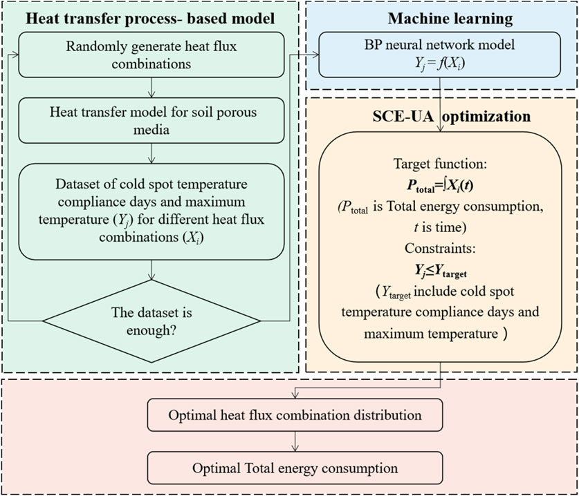
Figure 1. Flow chart of ISTD technology optimization.

2.2 Process-based heat transfer model

In this study, COMSOL Multiphysics 5.6 was used to create the heat transfer model for ISTD in porous media. COMSOL Multiphysics is a comprehensive numerical simulation program based on the finite element method (Mohamed et al., 2023). This software simulates physical phenomena by applying the solution of partial differential equations (single field) or systems of partial differential equations (multi-field).

For heat conduction model, the governing equation for the model of the transient heat conduction process for heat transfer in porous media is Equation 1 (Das et al., 2020).

$\rho C_{\mathrm{p}}\left(\frac{\mathrm{\partial }T}{\mathrm{\partial }t}+{\mathbf{u}}_{\text{trans}}·\nabla T\right)+\nabla ·\left({\mathbf{q}}_{\mathrm{c}}+{\mathbf{q}}_{\mathrm{r}}\right)=-\alpha T:\frac{\mathrm{d}S}{\mathrm{d}t}+M_{\mathrm{w}}(1)$

where ρ is the density [kg/m³], $C_{\mathrm{p}}$ is the specific heat capacity at constant stress [J/(kg·K)], T is the absolute temperature [K], t is the time [s], u_trans is the velocity vector of translational motion [m/s], q_c is the heat flux by conduction [W/m²], q_r is the heat flux by radiation [W/m²], α is the coefficient of thermal expansion [1/K], S is the second Piola–Kirchhoff stress tensor [Pa], and M_w contains additional heat sources [W/m³].

2.3 Machine learning procedure

In the 1980s, neural networks based on connectionist learning began to flourish, with the BP algorithm being the best known (Ma et al., 2021). The BP neural network is widely used in research areas such as air pollution (Chen et al., 2023a), soil pollution (Tao et al., 2019) and groundwater (Gharehbaghi et al., 2022). In the ISTD process, the heat flow, the cold spot temperature and the duration of its continuous application are important indicators that influence the efficiency of contaminant removal. However, in engineering practice, due to the complexity of the site and the limited remediation time, a more extensive construction approach is often chosen, which makes precise construction difficult and leads to energy waste. Furthermore, using only the process-based heat transfer model to exhaustively study the temperature variations at the cold spot under all heating conditions is computationally expensive. Machine learning offers a new approach to solve this dilemma. In machine learning modeling, evaluation metrics are typically used to assess the performance and generalization ability of the model. The aim is to train the model on the data set so that it can learn universal patterns that are applicable to all potential samples, thereby reducing the number of training errors and generalization errors to make accurate predictions for new samples. The most commonly used metric is the mean squared error (MSE), whose specific calculation formula is Equation 2:

$\text{MSE}=\frac{1}{n}{\displaystyle \sum _{i=1}^n}{\left(f\left(x_i\right)-y_i\right)}^2(2)$

where n is the sample number, f(x_i) is the predicted value, and y_i is the true value.

The coefficient of determination, which is also known as R-squared (R²), is a measure of goodness-of-fit for regression models and ranges from 0 to 1. A value closer to 1 implies a better fit of the model to the data. Equation 3 is the formula for calculating R² (Wang et al., 2021a):

$R^2=\frac{{\left(\sum \left(O_i-\overline{O}\right)\left(E_i-\overline{E}\right)\right)}^2}{\sum {\left(O_i-\overline{O}\right)}^2\sum {\left(E_i-\overline{E}\right)}^2}(3)$

where O_i is the ith measured data, E_i is the ith simulated data, $\overline{O}$ is the mean of the measured data, and $\overline{E}$ is the mean of the simulated data.

In this study, a BP neural network was selected to establish the relationship between heat flux, days of cold spot temperature compliance and maximum heating temperature based on the test results (Supplementary Table S1). The BP neural network consisted of an input layer, a hidden layer, and an output layer. In this study, the input layer consisted of 15 neurons corresponding to 15 different heat fluxes, and the output layer consisted of two neurons corresponding to the days of maintaining the cold spot temperature and the maximum temperature inside the heating unit. The total data were randomly divided into learning and test data, with 80% of the data used for training and 20% for testing.

To determine the optimal number of training samples, the number of hidden layers and the number of neurons in the hidden layer were determined by trial and error (Supplementary Table S2–S4). Finally, it was found that the optimal configuration for the BP neural network model is a hidden layer with 10 neurons. The final BP neural network model was obtained with a total of 1,715 samples, one hidden layer, and 10 neurons in the hidden layer. The BP neural network model was created using the Python-based open-source code TensorFlow. The sigmoid activation function was chosen, and the learning rate was set to 0.03. Supplementary Table S5 showed the specific model parameter settings. In this study, the primary input variables for ML training were the dynamic change of heat flux with time. Supplementary Table S6 showed the input variables used in the simulation, and the results of the tests.

2.4 SCE-UA optimization for energy consumption procedure

SCE-UA is a sophisticated shuffle evolution method developed by Qingyun Duan from the University of Arizona (Duan et al., 1994). It is characterized by high efficiency and flexibility and is a relatively widespread global optimization method. This method integrates a number of optimization techniques, such as random search and genetic algorithms, and is based on four core concepts to provide a reliable and robust approach for solving large complex optimization problems with high dimensionality and nonlinearity (Tolson and Shoemaker, 2007).

In this study, parameter settings for the SCE-UA algorithm started with the selection of a population size of p = 30, with each population containing m = 31 points, resulting in a total sample size of s = p × m = 930. These points were then sorted in ascending order by their function values and stored in the array D. Each population was evolved using the competitive complex evolution (CCE) algorithm and then shuffled and assigned to new populations to facilitate information sharing (Jun-wei et al., 2022). The evolution and transformation process was repeated until the convergence condition was met, at which point the process was terminated. Other parameters used in the SCE-UA optimization steps were the maximum number of function evaluations allowed during the optimization process (n_max = 600,000) and the maximum number of evolutionary cycles before convergence (k_stop = 100).

2.5 Implementation of the model framework

2.5.1 Model assumptions

The construction of the heat transfer model for porous media in this study is based on the following assumptions (Wang et al., 2019).

1. It is assumed that the soil is homogeneous and isotropic and that its type does not change along the direction of the heat source (in reality, the soil is a non-uniform and non-isotropic porous material). This assumption has a negligible effect on thermal conductivity, as the differences in thermal conductivity between different soil types are limited.

2. During heating, heat is mainly transferred by conduction.

3. The skeleton of the soil unit does not undergo any phase change or deformation during the heating process.

4. The influence of contaminants on the temperature field can be neglected.

5. The temperature is the same for soil on the same cross-section and the physical properties remain constant.

2.5.2 Model construction and parameter settings

In engineering remediation, it is possible to achieve uniform heating of the entire contaminated area through the strategic placement and density of heating rods, improving the effectiveness of thermal desorption and reducing the cost of transporting and treating the soil. The heating wells are usually arranged in a regular hexagonal or equilateral triangular pattern (see Supplementary Figure S1), with a spacing between the heating rods of between 2 and 6 m. The heating boreholes can be arranged in the same place as the extraction wells for remediation.

The arrangement of the heating rods is similar to the arrangement of the heating wells. In this study, a regular hexagonal arrangement with a distance of 2 m between the heating rods was chosen. A thermal remediation unit cell based on the symmetry principle was used as the object of investigation. The simulated soil unit is a regular pentagonal prism with a side length of 1.73 m for the base of the equilateral triangle and a height of 25 m for the pentagonal prism. The top layer is the insulation layer with a thickness of 0.5 m, followed by the soil heating layer with a height of 9.5 m. To ensure the rationality of the model simulation and the scientific definition of the lower boundary, the middle layer was extended downwards by 15 m to form the lower boundary layer of the soil unit. The heating rods are cylindrical with a radius of 0.07 m and a height of 10.5 m and serve as a heat source to increase the soil temperature. To ensure a fast and effective temperature response at the cold spot temperature, the heating rods are positioned at a depth of 0.5 m in the insulating layer, 9.5 m in the middle layer and 0.5 m in the bottom layer of the soil. The diagram of the setup is shown in Supplementary Figure S2a. Based on the assumptions in Section 2.5.1, the porous media heat transfer model was created using COMSOL Multiphysics 5.6 software, and then the area was subjected to grid partitioning. After grid partitioning, the simulation domain contained a total of 32,583 domain elements, 3,058 boundary elements and 577 boundary elements (Supplementary Figure S2b).

The thermal remediation unit cell was determined on the basis of the symmetry principle. Therefore, the boundary conditions were set such that the lateral sides of the soil unit were considered fully adiabatic, with the lateral boundaries set as flux-free boundaries and the bottom boundary as thermally insulated. The convective heat flux was chosen as the upper boundary condition. The initial temperature of the heating rods was set at 293.15 K, neglecting the influence of factors such as moisture evaporation. Considering the heat losses and the influence of the upper and lower thermal boundaries, a boundary influence zone of 2 m above and below the heating rods was chosen. During the heat transfer process, the temperature varies with time, so a transient calculation method was used to simulate the process in this study. The main focus of this study was on the spatio-temporal variation of the temperature field around the heating rods in the thermal remediation unit cell, with heat conduction being the dominant factor. Reference was made to relevant literature research to determine appropriate model parameters (Wang et al., 2019), and the model parameters were set accordingly, as shown in Supplementary Table S7.

For volatile contaminants, the target heating temperature is set at the boiling point of the contaminant, with sufficient heat flux required to heat the contaminated soil to its boiling point to remove the contaminant. The target heating temperature generally refers to the cold spot temperature of the soil in the remediation area. In this study, benzene compounds were used as target contaminants, which typically represent a mixture containing benzene, toluene, ethylbenzene, and o-, m-, p-xylene, abbreviated as BTEX. And given the presence of azeotropic phenomena (Zhao et al., 2014), the cold spot temperature was set at 100 °C. The heating time usually depends on factors such as the duration of the remediation project, the type of contaminants, the extent of the remediation and the number of heating rods. Based on experience from engineering cases both domestically and abroad, the heating time is usually between 30 and 90 days, with some large-scale contaminated sites taking up to 130 days to heat up (Li et al., 2017). In this study, the heat-up time was set at 75 days, taking into account the actual case constellations and the model test results.

2.5.3 Description of model scenarios

Different heat fluxes lead to variations in temperature distribution, and temperature has a significant effect on the removal of contaminants. Therefore, two scenarios were considered in this study. In scenario 1, the heat transfer performance and temperature distribution within a thermal remediation unit cell were simulated under constant heat flux conditions. Supplementary Figure S3 showed the sensitivity analysis results of model parameters and initial conditions. Results showed that initial temperature changes have little effect on the outcomes, while the influences of soil thermal conductivity and specific heat capacity on heat transfer dynamics were relatively greater compared to the initial temperature. Accurate measurement of these thermal properties is therefore critical for field applications. In scenario1, the quantitative relationship between constant heat flux and the cold spot temperature as well as the maximum temperature within the temperature field was investigated. In practise, however, in order to achieve the remediation goal within the limited remediation period, the energy input is often increased so that the target temperature can be reached quickly and the contaminants removed. However, this leads to a considerable waste of energy and increased remediation costs. In order to reduce costs and improve the efficiency of ISTD, the heat transfer performance and temperature distribution within a typical soil heating unit under variable heat flux conditions were investigated in scenario 2.

In Scenario 2, the heat flux was assumed to be a piecewise function varying with time (Supplementary Figure S4). Although physically unrealistic, to populate the machine learning parameter space, a total of 1,715 sets of data were generated using Python’s random function with each set covering a total heating period of 75 days. Within each set, the heat flux varied every 5 days, resulting in 15 different heat flux values for each dataset. To consider various scenarios comprehensively, including extreme conditions, the heat flux range was set from 1 to 20 W/cm². Subsequently, the randomly generated heat flux values were integrated over time to obtain the total energy consumption. These 1,715 sets of varied heat flux data (a matrix of 1,715 × 15 heat flux combinations) served as input variables. The output variables were the cold spot temperature and the maximum temperature within a thermal remediation unit cell simulated using the porous media heat transfer model during the heating period. It is important to note that the maximum temperature refers to the maximum temperature within the heating unit, and in most cases, this value does not exceed the material’s maximum tolerance temperature. Because the heat flux combinations in Scenario 2 were entirely randomly obtained, to prevent extreme situations, a limitation was imposed on the maximum temperature to ensure the rationality of the simulation results. Hence, considering the material’s tolerance temperature for the heating pipes, the maximum temperature was set not to exceed 1,200 K. All these randomly generated samples and corresponding simulation results were used as the sample dataset for subsequent machine learning.

3 Results and discussion

3.1 Optimization results of soil ISTD technology under the constant heat flux scenario

Based on 75-day simulation results, this study explored the interaction between heat flux and the time it takes to reach the desired cold spot temperature during the ISTD process at the site. To illustrate this relationship, Figure 2 shows the time evolution of the cold spot temperature and the maximum temperature within the heating unit under constant heat flux conditions.

Figure 2

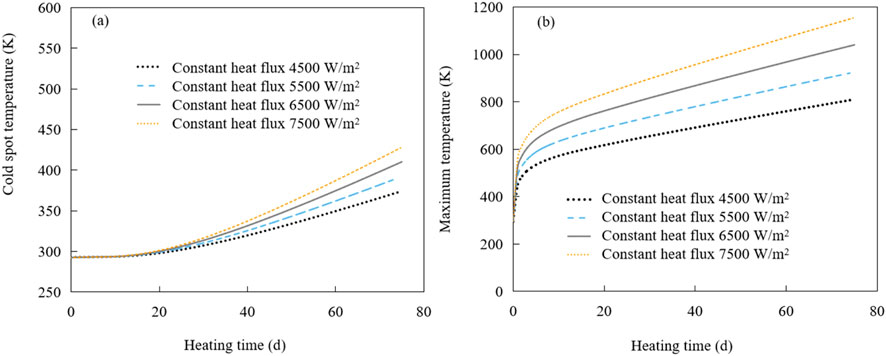
Figure 2. Plot of the cold spot temperature (a) and the maximum temperature (b) changing with the heating time under different constant heat flux conditions.

During the initial approximately 30 days of the heating period, the cold spot temperature within the heating unit gradually increased (Figure 2a). This gradual increase was due to the combined effects of the distance between the coldest point and the heat source and the thermal conductivity of the surrounding soil. These factors resulted in a delayed heating effect that led to a measured and controlled temperature rise. As the heating period progressed, the cold spot temperature rose steadily, with the increased heat flux leading to an exponential rise in temperature. The relationship between the maximum temperature within the heating unit and the heating time under different constant heat flux conditions is shown in Figure 2b. In contrast to the cold spot temperature, the maximum temperature rose rapidly in the initial phase and quickly reached the target temperature. With prolonged heating, the temperature increase slowed down due to heat loss in both lateral and longitudinal directions (Supplementary Figure S5). Overall, both the cold spot temperature and the maximum temperature at constant heat flux showed a direct correlation with the increase in heat flux. Nevertheless, the delayed heat conduction and the heat losses led to a delayed increase of the cold spot temperature compared to the maximum temperature near the heat source.

Figures 3, 4 illustrate the effects of heat conduction and temperature fluctuations by showing a cross-section of the temperature distribution at different heating times. Figures 3a–c show cross-sections at heating times of 5, 40 and 75 days with a heat flux of 4,500 W/m². In this setting, due to the cold spot temperature attained the target only on the 74th day due to the relatively low heat flux. At this time, when the maximum temperature within the site was reached 798.59 K. Furthermore, as the heating time increased, the temperature near the heat source was significantly higher than that near the distant heat source in both the longitudinal and transverse directions. This indicates that the distant heat source area requires more time and energy to reach the temperature of the cold spot. Therefore, special attention should be given to changes in the cold spot temperature during practical remediation engineering.

Figure 3

Figure 3. Temperature field cross sections at different times with the constant heat fluxes of 4,500 W/m² (a–c) and 5,500 W/m² (d–f).

Figure 4

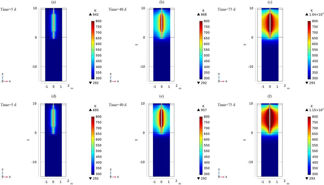
Figure 4. Temperature field cross sections at different times with the constant heat fluxes of 6,500 W/m² (a–c) and 7,500 W/m² (d–f).

The effect of a higher heat flux becomes clear when comparing Figures 3a–f, where the surroundings of the heat source experience a faster temperature rise, which increases the overall heat efficiency. When the heat flux was increased to 5,500 W/m², the target heating temperature was reached on the 70th day, and the maximum temperature within the site also increased to 910.93 K. This observation shows that a higher heat flux leads to a shorter time to reach the target heating temperature and improves the overall heating efficiency.

Figures 4a–f show cross-sections of the temperature distribution at heat fluxes of 6,500 W/m² and 7,500 W/m² respectively. The temperature rose steadily as the heating time progressed. A faster temperature rise was recorded near the heat source, which led to a higher heating efficiency. In the areas away from the heat source, however, the temperature increase was slower, especially beyond the depth range of the heating rod, where the heating effect was less pronounced. In addition, both the longitudinal and transverse heat conduction areas increased with increasing heating time, and the heat flux also had a cumulative effect on the heat conduction area. Higher heat fluxes led to a wider heat conductivity range. These results highlight the importance of the depth of the heating rod, the variation in temperature at the cold spot and the intensity of the heat flux, all of which influence the extent of ISTD remediation. Consequently, these factors must be carefully considered in practical engineering remediation efforts.

The heating process of a thermal remediation unit cell was simulated with a constant heat flux of 4,000 to 8,000 W/m² using preliminary estimates and trial-and-error methods (Supplementary Figure S6). The results showed that at 4,000 W/m² the temperature of the cold spot did not reach the target temperature, which required a higher heat flux. At 4,500 W/m², the cold spot temperature reached the target temperature in only 1 day with a peak temperature of 798.59 K. A higher heat flux led to a longer time to reach the target temperature. At 8,000 W/m² it took 23 days, but the temperature exceeded 1,200 K and thus violated the target. In summary, at a constant heat flux, the optimum range of 4,500 to 8,000 W/m² proves to be a suitable compromise that effectively balances both the time required to reach the target temperature and compliance with the maximum temperature specification.

To enable a more meaningful comparison with variable heat flux scenarios, data fitting was performed as part of this study to establish a mathematical relationship (Supplementary Figure S7) between total energy consumption and the duration required to reach the target heating temperature while maintaining the maximum temperature target (≤1,200 K). The mathematical relationship embodies the optimal synergy between the total energy consumption and the time to reach the desired heating temperature in a constant heat flux scenario. For practical technical applications, where the typical time to reach the target temperature is around 10 days, the function shown in Supplementary Figure S7 gives a total energy consumption of 17,084.3 kWh. These results can provide valuable guidance for practical implementation and support the pursuit of energy-efficient and unrestricted remediation measures.

3.2 Optimization results of soil ISTD technology under a variable heat flux scenario

In real engineering remediation is frequently faced with suboptimal parameters such as heating time and heat flux, leading to substantial energy inefficiency and elevated project costs. As a result, the variable heat flux scenario explores diverse heat flux combinations under dynamic conditions. It aims to quantitatively estimate the optimal heating time and energy consumption during the ISTD process, thereby enhancing the engineering operational efficiency in the implementation of ISTD technology.

As already explained in Section 2.5.3, the variable heat flux scenario assumes a time-varying piecewise function for heat flux. A total of 1,715 distinct heat flux combinations were generated using Python’s random function through testing (Supplementary Table S2). For each combination, the porous media heat transfer model simulated temperature distribution, yielding data on the days required to reach the target heating temperature and the maximum temperature within the heating unit. Out of these 1,715 cases, 1,372 were allocated for training the BP neural network model, while the remaining 343 were used for testing. After training and testing (Table 1), the R² consistently exceeded 0.85 for both datasets, and the MSE values approached zero, indicating that the BP neural network model exhibited strong regression performance for both training and testing (Wang et al., 2021a). This performance made it well suited for subsequent optimization endeavors.

Table 1

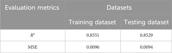
Table 1. Table of the BP neural network model indicator evaluation.

Subsequently, the well-trained BP neural network model was integrated into the SCE-UA global optimization method to find the optimal combinations of heat flux and minimize the total energy consumption while satisfying the conditions of reaching the target heating temperature for the cold spot and limiting the maximum temperature. Figure 5 shows the changes of the cold spot temperature (Figure 5a) and the maximum temperature (Figure 5b) over time under the variable heat flux conditions after the optimization prediction.

Figure 5

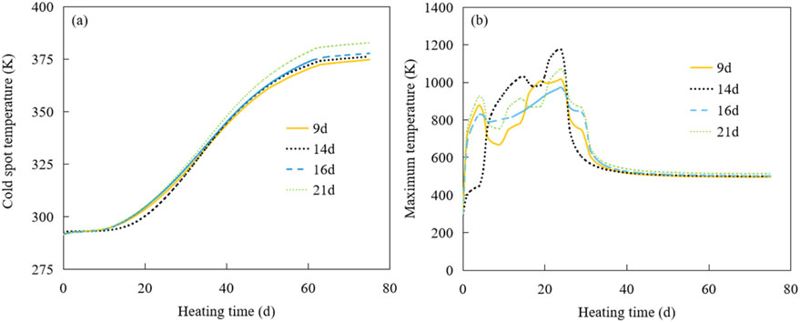
Figure 5. Plot of the cold spot temperature (a) and the maximum temperature (b) changing with the heating time under the variable heat flux conditions. The cases of 9 days, 14 days, 16 days, and 21 days correspond to the number of days it takes for the cold spot temperature to reach the target temperature in each respective case.

The results shown in Figure 5a indicate a behavior of the temperature of the cold spot during the first heating phases. This temperature, which was similar to that observed in the constant heat flux scenario, was characterized by a delayed rise due to heat conduction effects. However, the variable heat flux conditions resulted in an earlier increase in cold spot temperature, which started around day 20 and stabilized between day 20 and day 40. As the heating time increased, the cold spot temperature continued to rise, finally stabilizing around day 60 in the range of 375–383 K. Figure 5b shows the fluctuations of the maximum temperature near the heat source inside the heating unit. Initially, there was an upward trend, followed by a subsequent decline, eventually leading to a stable and gradual transition over time. These patterns were mainly influenced by the distribution of heat flux combinations and the effects of heat losses. When examining the distribution of the optimized heat flux combinations (Supplementary Table S8), a clear pattern emerged, characterized by higher heat flux values in the early heating phases and lower heat flux values in the later phases. The higher heat flux in the early phases accelerated heat conduction and enabled a rapid temperature rise to reach the target temperature. Conversely, the temperature of the cold spot rose later due to the delayed heat conduction. As the heating time increased, only a lower heat flux was required in the later phases to maintain the temperature of the cold spot at or above the target temperature and achieve effective remediation of the contaminated soil.

Figures 6, 7 show cross-sections of the temperature distribution resulting from the optimization and depict scenarios in which the cold spot temperature reaches the target within 9, 14, 16 and 21 days under variable heat flux conditions. Figures 6a–c, which represents the case where the cold spot temperature reaches the target in 9 days, shows a strategy with higher heat flux in the initial phase. On the 5th day, the maximum temperature increased to 836 K, with the heating concentrated on the rods to reach the target temperature quickly. In contrast to the scenario with a constant heat flux, the maximum temperature did not rise continuously as the heating time progressed. Instead, there was a slight decrease around the 40th day, which was attributed to a significant reduction in heat flux and total energy consumption. Thereafter, until the 75th day, the heating range remained relatively constant, while the maximum temperature decreased by 21 K.

Figure 6

Figure 6. Temperature distribution cross sections of the target heating temperature reached in 9 days (a–c) and 16 days (d–f) under the variable heat flux scenario.

Figure 7

Figure 7. Temperature distribution cross sections of the target heating temperature reached in 14 days (a–c) and 21 days (d–f) under the variable heat flux scenario.

The evolving temperature distribution patterns for the cases in which the cold spot temperature reached the target in 14, 16 and 21 days mirrored those of the 9-day scenario. In all cases, the maximum temperature initially rose and then fell again, while the heated area expanded as the heating time progressed. It is worth noting that there was no direct correlation between the number of days required to reach the target temperature and the maximum temperature increase. For example, on the fifth day of the heating cycle, the maximum temperatures for the scenarios with 9, 14, 16 and 21 days to reach the target temperature were 836 K, 538 K, 666 K and 905 K, respectively. This discrepancy could be due to the stochastic nature of the global optimization algorithm and the high dimensionality of the data set, which lead to deviations in the optimal heat flux combinations. Despite these discrepancies, the overall trend of the optimized heat flux combinations showed an initial increase followed by a decrease, all successfully meeting the targets when validated with the regression model.

Table 2 shows the optimized distribution of heat flux combinations over different time periods to reach the target temperature of the cold spot. The data shown in Table 2 show a consistent trend: as the number of days required to reach the desired heating temperature increases, so does the total energy consumption, regardless of whether it is a variable or constant heat flux scenario. This logical correlation follows the principle that maintaining a elevated temperature over a longer period of time requires a higher energy input. Over the 75-day heating cycle, a relatively high heat flux is typically used for the first 30 days, followed by a significant reduction. This pattern results from the need to maintain a elevated heat flux in the initial phase in order to accelerate the achievement of the target temperature. Once the target temperature has been reached, factors such as the delay in heat transfer and the diffusion of residual heat at high temperatures play an important role. Therefore, a moderate heat flux is sufficient to keep the temperature above the set threshold. From the perspective of energy efficiency, the heat flux combination that cold spot temperature compliance days of 19 demonstrates the most favorable trade-off compared to other optimization results (e.g., 7-days). This solution reduces energy consumption by 13% while still meeting the remediation target (Table 3). This approach optimizes energy use and thus increases the efficiency of the remediation process.

Table 2

Table 2. Optimal heat flux combination distribution.

Table 3

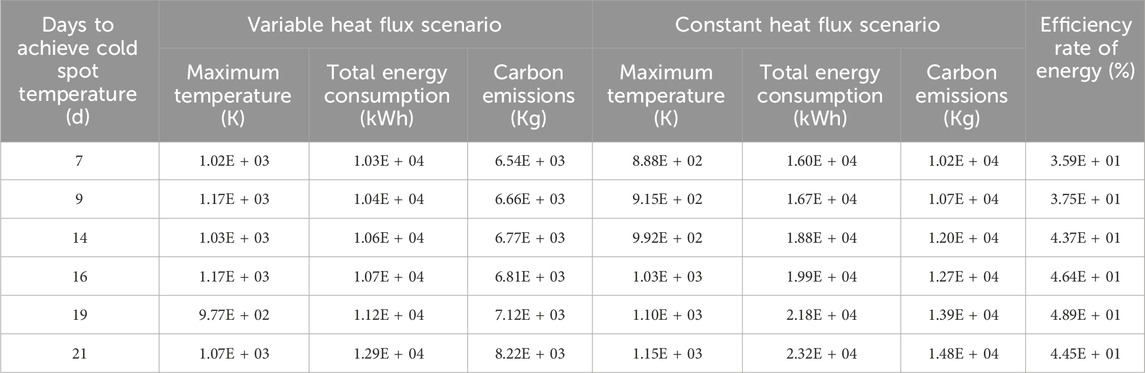
Table 3. Optimization results for varying cold spot temperature compliance days across different scenarios.

Table 3 shows the optimization results for different scenarios with different days for maintaining the cold spot temperature. The variable heat flux scenario consistently consumed less total energy than the constant heat flux scenario, achieving savings between 35.93% and 48.86%. These results highlight the importance of optimizing heat flux distribution in mitigating the environmental impact of soil remediation measures. Carbon emissions were estimated based on relevant studies (Ecological Environment Department of Guangdong Province, 2022) and ranged from 10,207.38 kg to 14,802.41 kg for the constant heat flux scenario and 6,540.06–8,218.73 kg for the variable heat flux scenario. Notably, the variable heat flux approach significantly reduces carbon emissions compared to the constant heat flux scenario, highlighting the potential benefits of adaptive energy allocation in minimizing environmental impacts. This optimization not only increases energy efficiency and cost effectiveness, but also fits seamlessly into broader sustainability goals by reducing carbon emissions.

3.3 Potential limitation

In this study, despite the significant progress made in proposing an optimized design method for temporally variable heating curves in ISTD of contaminated soils by integrating machine learning with a process-based heat transfer model, there are several potential limitations that warrant attention.

1. Machine learning technique limitations. In the past decade, the development of big data technology has promoted research in physical information machine learning, hybrid modeling, and adaptive control in thermal remediation (Cai et al., 2021; Zobeiry and Humfeld, 2021). These research efforts have been applied to optimize the energy efficiency of heat pump systems (Olabi et al., 2023), design heat sinks for electronic components (Hennigh et al., 2021), and explore various application scenarios (e.g., fault detection and diagnostics) (Chen et al., 2023b). The use of a BP neural network, while meeting current research requirements (achieving R² = 0.8529 on validation sets), may not leverage advanced ML innovations (e.g., deep learning, ensemble techniques) that could improve prediction accuracy and generalization. Upgrading to more sophisticated models in future work could enhance the surrogate model’s efficiency, especially for high-dimensional time-series optimization tasks.

2. Simplified soil property assumptions. In this study, the model relied on homogeneous and isotropic assumptions for soil properties, which may not fully reflect real-world site heterogeneity. Although soil heterogeneity (e.g., porosity, permeability) has minimal impact on pure heat conduction processes compared to fluid flow, it can influence heat dynamics in complex subsurface environments (Wang et al., 2019). Future studies should incorporate key soil properties (e.g., texture, organic matter content, and moisture variability) as well as contaminant-specific behaviors (such as thermal degradation and mobility) to enhance model applicability to diverse site conditions. Furthermore, the omission of terrain variability in this study represents a limitation. Future work should evaluate how different terrains affect ISTD performance, particularly in heterogeneous soil.

3. Multi-physical process integration limitations. This study focused on heat conduction optimization while simplifying or excluding processes like thermal degradation of specific contaminants (e.g., PAHs, VOCs) and contaminant mobility. Full coupling of these multi-physical processes would increase model complexity and uncertainty, but neglecting them may limit predictions for sites with complex contaminant profiles. Future work should explore hybrid modeling frameworks that balance computational efficiency with mechanistic detail to address real-world remediation complexities.

4. Uncertainties and experiment limitations. The results presented in this study are primarily based on simulation models without field or laboratory experimental validation due to high cost and time consumption. Thus, they are subject to the inherent uncertainties of the modeling approach. These include structural uncertainties arising from the simplification of complex real-world geology, parametric uncertainties associated with the thermal properties of materials, numerical uncertainties introduced by the discretization of the computational domain and scenario uncertainties due to the use of idealized boundary conditions (Wang et al., 2019). In addition, the absence of field or laboratory validation, while justified by resource constraints, means the quantitative accuracy of the results is uncertain. Consequently, the model outputs are best viewed as a demonstration of a promising trend. Future studies should validate the optimization strategy through pilot-scale experiments and assess its performance under variable site conditions (Gong et al., 2018).

5. Scope of Optimization Variables. Previous scholars have conducted similar numerical modeling studies, but these were limited to numerical modeling alone and did not integrate machine learning or optimization algorithms to refine remediation strategies (Wang et al., 2019; Ganguly et al., 2017). The current framework optimizes heating temperature and time series but does not address other optimization variables (e.g., well spacing, heat flux patterns). Expanding the optimization scope to include multi-variable interactions could further enhance energy efficiency.

4 Conclusion

ISTD technology is characterized by the fact that it relies on an extensive and energy-intensive thermal system, which results in elevated operating costs and significant energy consumption. Therefore, it is crucial to make precise and reliable optimization predictions for energy demand and operating time. To effectively address this challenge, an optimization methodology for ISTD ground technology is presented in this study. This approach integrates machine learning with a process-based heat transfer model to determine the optimal allocation of heat flux that meets the criteria of achieving the desired duration for the target cold spot temperature while minimizing the total energy consumption. Unlike References (Xu et al., 2022) and (Wang et al., 2021b), which focused on numerical modeling and laboratory experiments respectively, this study integrates machine learning with process-based modeling. By employing surrogate models to optimize heating time series, the proposed approach offers a novel perspective for site remediation, particularly in the context of ISTD technology. However, this technology is not designed for on-site real-time control. Rather, it optimizes the time sequence during the process design phase before site entry. This optimization is dynamic, not static. During the implementation of site remediation, the preliminary optimization results can be further integrated with dynamic feedback data collected by on-site sensors. Through iterative integration and re-optimization, a more ideal remediation effect can be achieved.

In this proposed methodology, a heat transfer model for porous media is used to simulate the spatio-temporal trends in the temperature fields of the thermal remediation unit cell exposed to different heat flux combinations. Compared with traditional enumeration-based numerical simulation optimization methods (e.g., parameter optimization techniques), the optimization framework developed in this study possesses the capability to handle high-dimensional variables, enabling effective dynamic optimization of time-series parameters. Additionally, the introduction of ML surrogate models significantly reduces computational costs, making optimization of high-dimensional operational variables feasible, particularly demonstrating technical advantages in time-series optimization scenarios. This methodology establishes a scientific framework for the application of ISTD technology in site remediation, forming a robust basis for strategic decision-making in the domain of soil remediation and environmental management. Future research should focus more on the composite effects of multiple factors in TCH and develop multi-field coupling models through the combination of numerical simulation and in-situ experiments. Accurate characterization and prediction of entire TCH process can improve remediation efficiency, reduce energy costs, and achieve sustainable low-carbon remediation.

Data availability statement

The original contributions presented in the study are included in the article/Supplementary Material, further inquiries can be directed to the corresponding authors.

Author contributions

XW: Conceptualization, Formal Analysis, Methodology, Software, Validation, Writing – original draft. YL: Data curation, Formal Analysis, Investigation, Validation, Visualization, Writing – original draft. YT: Methodology, Software, Supervision, Writing – review and editing. BZ: Data curation, Investigation, Visualization, Writing – original draft. QL: Funding acquisition, Supervision, Writing – review and editing. SX: Funding acquisition, Supervision, Writing – review and editing. YZ: Project administration, Writing – review and editing. TZ: Project administration, Writing – review and editing. QY: Supervision, Writing – review and editing. RL: Conceptualization, Funding acquisition, Methodology, Software, Supervision, Writing – review and editing.

Funding

The authors declare that financial support was received for the research and/or publication of this article. This research was supported by National key research and development program (project No: 2024YFC3712504) and the Shenzhen Sustainable Development Project, China (KCXFZ20240903094007010).

Conflict of interest

Authors XW and SX were employed by Shenzhen Technology Institute of Urban Public Safety Co Ltd. Authors YZ and TZ were employed by Wisdri City Environment Protection Engineering Limited Company.

The remaining authors declare that the research was conducted in the absence of any commercial or financial relationships that could be construed as a potential conflict of interest.

Generative AI statement

The authors declare that no Generative AI was used in the creation of this manuscript.

Any alternative text (alt text) provided alongside figures in this article has been generated by Frontiers with the support of artificial intelligence and reasonable efforts have been made to ensure accuracy, including review by the authors wherever possible. If you identify any issues, please contact us.

Publisher’s note

All claims expressed in this article are solely those of the authors and do not necessarily represent those of their affiliated organizations, or those of the publisher, the editors and the reviewers. Any product that may be evaluated in this article, or claim that may be made by its manufacturer, is not guaranteed or endorsed by the publisher.

Supplementary material

The Supplementary Material for this article can be found online at: https://www.frontiersin.org/articles/10.3389/fenvs.2025.1730352/full#supplementary-material

Abbreviations

ISTD, In situ soil thermal desorption; PAHs, Polycyclic aromatic hydrocarbons; VOCs, Volatile organic pollutants; SVOCs, Semi-volatile organic pollutants; OCPs, Organochlorine pesticides; PCBs, Polychlorinated biphenyls; ERH, Electrical resistive heating; TCH, Thermal conduction heating; SEE, Steam-enhanced extraction; BP, Backpropagation; SCE-UA, The shuffled complex evolution method developed at the University of Arizona algorithm; MSE, The mean squared error; R², R-squared; CCE, The competitive complex evolutionalgorithm; BTEX, Benzene, toluene, ethylbenzene, and o-, m-, p-xylene.

References

Busto, Y., Cabrera, X., Tack, F. M. G., and Verloo, M. G. (2011). Potential of thermal treatment for decontamination of mercury containing wastes from chlor-alkali industry. J. Hazard. Mater. 186 (1), 114–118. doi:10.1016/j.jhazmat.2010.10.099

PubMed Abstract | CrossRef Full Text | Google Scholar

Cai, S., Mao, Z., Wang, Z., Yin, M., and Karniadakis, G. E. (2021). Physics-informed neural networks (PINNs) for fluid mechanics: a review. Acta Mech. Sin. 37 (12), 1727–1738. doi:10.1007/s10409-021-01148-1

CrossRef Full Text | Google Scholar

Cao, H.-L., Cai, F.-Y., Jiao, W.-B., Wang, Y., Liu, C., Zhang, N., et al. (2018). Microwave-induced decontamination of mercury polluted soils at low temperature assisted with granular activated carbon. Chem. Eng. J. 351, 1067–1075. doi:10.1016/j.cej.2018.06.168

CrossRef Full Text | Google Scholar

Chen, R., Teng, Y., Chen, H., Yue, W., Su, X., Liu, Y., et al. (2021). A coupled optimization of groundwater remediation alternatives screening under health risk assessment: an application to a petroleum-contaminated site in a typical cold industrial region in Northeastern China. J. Hazard. Mater. 407, 124796. doi:10.1016/j.jhazmat.2020.124796

PubMed Abstract | CrossRef Full Text | Google Scholar

Chen, J., Liu, Z., Yin, Z., Liu, X., Li, X., Yin, L., et al. (2023a). Predict the effect of meteorological factors on haze using BP neural network. Urban Clim. 51, 101630. doi:10.1016/j.uclim.2023.101630

CrossRef Full Text | Google Scholar

Chen, Z. L., O’Neill, Z., Wen, J., Pradhan, O., Yang, T., Lu, X., et al. (2023b). A review of data-driven fault detection and diagnostics for building HVAC systems. Appl. Energy. 339, 121030. doi:10.1016/j.apenergy.2023.121030

CrossRef Full Text | Google Scholar

Chen, Z., Chen, Z., Li, Y., Zhang, R., Liu, Y., Hui, A., et al. (2024). A review on remediation of chlorinated organic contaminants in soils by thermal desorption. J. Ind. Eng. Chem. 133, 112–121. doi:10.1016/j.jiec.2023.12.022

CrossRef Full Text | Google Scholar

Das, D., Singapuri, C., and Dwivedi, A. (2020). Experimental determination of buoyancy induced convection heat transfer characteristics in a rectangular cavity with cylindrical porous medium fixed between pin fins. Heat. Mass Transf. 56 (4), 1293–1306. doi:10.1007/s00231-019-02767-y

CrossRef Full Text | Google Scholar

Douay, F., Roussel, H., Pruvot, C., Loriette, A., and Fourrier, H. (2008). Assessment of a remediation technique using the replacement of contaminated soils in kitchen gardens nearby a former lead smelter in Northern France. Sci. Total Environ. 401 (1), 29–38. doi:10.1016/j.scitotenv.2008.03.025

PubMed Abstract | CrossRef Full Text | Google Scholar

Duan, Q., Sorooshian, S., and Gupta, V. K. (1994). Optimal use of the SCE-UA global optimization method for calibrating watershed models. J. Hydrol. 158 (3), 265–284. doi:10.1016/0022-1694(94)90057-4

CrossRef Full Text | Google Scholar

Ecological Environment Department of Guangdong Province (2022). Guidelines for carbon dioxide emission reporting of enterprises (Units) in Guangdong Province. Guangzhou, China: Ecological Environment Department of Guangdong Province. Available online at: http://gdee.gd.gov.cn/attachment/0/483/483550/3836469.pdf (Accessed March 4, 2022).

Google Scholar

Ganguly, S., Kumar, M. S. M., Date, A., and Akbarzadeh, A. (2017). Numerical investigation of temperature distribution and thermal performance while charging-discharging thermal energy in aquifer. Appl. Therm. Eng. 115, 756–773. doi:10.1016/j.applthermaleng.2017.01.009

CrossRef Full Text | Google Scholar

Gharehbaghi, A., Ghasemlounia, R., Ahmadi, F., and Albaji, M. (2022). Groundwater level prediction with meteorologically sensitive Gated Recurrent Unit (GRU) neural networks. J. Hydrol. 612, 128262. doi:10.1016/j.jhydrol.2022.128262

CrossRef Full Text | Google Scholar

Giannis, A., Nikolaou, A., Pentari, D., and Gidarakos, E. (2009). Chelating agent-assisted electrokinetic removal of cadmium, lead and copper from contaminated soils. Environ. Pollut. 157 (12), 3379–3386. doi:10.1016/j.envpol.2009.06.030

PubMed Abstract | CrossRef Full Text | Google Scholar

Gong, Y., Zhao, D., and Wang, Q. (2018). An overview of field-scale studies on remediation of soil contaminated with heavy metals and metalloids: technical progress over the last decade. Water Res. 147, 440–460. doi:10.1016/j.watres.2018.10.024

PubMed Abstract | CrossRef Full Text | Google Scholar

Han, C., Zhu, X., Xiong, G., Gao, J., Wu, J., Wang, D., et al. (2023). Quantitative study of in situ chemical oxidation remediation with coupled thermal desorption. Water Res. 239, 120035. doi:10.1016/j.watres.2023.120035

PubMed Abstract | CrossRef Full Text | Google Scholar

Hennigh, O., Narasimhan, S., Nabian, M. A., Subramaniam, A., Tangsali, K., Fang, Z., et al. (2021). NVIDIA SimNet™: an AIaccelerated multi-physics simulation framework. In: International conference on computational science. Berlin, Germany: Springer. p. 447–461.

Google Scholar

Jiang, Y., Wang, H., Lei, M., Hou, D., Chen, S., Hu, B., et al. (2021). An integrated assessment methodology for management of potentially contaminated sites based on public data. Sci. Total Environ. 783, 146913. doi:10.1016/j.scitotenv.2021.146913

PubMed Abstract | CrossRef Full Text | Google Scholar

Jun-wei, T. A. N., Qing-yun, D., Wei, G., and Zhen-hua, D. I. (2022). Differences in parameter estimates derived from various methods for the ORYZA (v3) model. J. Integr. Agric. 21 (2), 375–388. doi:10.1016/s2095-3119(20)63437-2

CrossRef Full Text | Google Scholar

Krol, M. M., Johnson, R. L., and Sleep, B. E. (2014). An analysis of a mixed convection associated with thermal heating in contaminated porous media. Sci. Total Environ. 499, 7–17. doi:10.1016/j.scitotenv.2014.08.028

PubMed Abstract | CrossRef Full Text | Google Scholar

Li, X., Jiao, W., Xiao, R., Chen, W., and Liu, W. (2017). Contaminated sites in China: countermeasures of provincial governments. J. Clean. Prod. 147, 485–496. doi:10.1016/j.jclepro.2017.01.107

CrossRef Full Text | Google Scholar

Ma, Y., Li, L., Yin, Z., Chai, A., Li, M., and Bi, Z. (2021). Research and application of network status prediction based on BP neural network for intelligent production line. Procedia Comput. Sci. 183, 189–196. doi:10.1016/j.procs.2021.02.049

CrossRef Full Text | Google Scholar

Mahar, A., Wang, P., Ali, A., Awasthi, M. K., Lahori, A. H., Wang, Q., et al. (2016). Challenges and opportunities in the phytoremediation of heavy metals contaminated soils: a review. Ecotoxicol. Environ. Saf. 126, 111–121. doi:10.1016/j.ecoenv.2015.12.023

PubMed Abstract | CrossRef Full Text | Google Scholar

Mohamed, Y. S., Hozien, O., Sorour, M. M., and El-Maghlany, W. M. (2023). Heat transfer simulation of nanofluids heat transfer in a helical coil under isothermal boundary conditions using COMSOL multiphysics. Int. J. Therm. Sci. 192, 108396. doi:10.1016/j.ijthermalsci.2023.108396

CrossRef Full Text | Google Scholar

Moon, D. H., Grubb, D. G., and Reilly, T. L. (2009). Stabilization/solidification of selenium-impacted soils using Portland cement and cement kiln dust. J. Hazard. Mater. 168 (2), 944–951. doi:10.1016/j.jhazmat.2009.02.125

PubMed Abstract | CrossRef Full Text | Google Scholar

O'Brien, P. L., DeSutter, T. M., Casey, F. X. M., Khan, E., and Wick, A. F. (2018). Thermal remediation alters soil properties – a review. J. Environ. Manage. 206, 826–835. doi:10.1016/j.jenvman.2017.11.052

PubMed Abstract | CrossRef Full Text | Google Scholar

Olabi, A. G., Haridy, S., Sayed, E. T., Radi, M. A., Alami, A. H., Zwayyed, F., et al. (2023). Implementation of artificial intelligence in modeling and control of heat pipes: a review. Energies 16, 760. doi:10.3390/en16020760

CrossRef Full Text | Google Scholar

Rehman, Z. u., Junaid, M. F., Ijaz, N., Khalid, U., and Ijaz, Z. (2023). Remediation methods of heavy metal contaminated soils from environmental and geotechnical standpoints. Sci. Total Environ. 867, 161468. doi:10.1016/j.scitotenv.2023.161468

PubMed Abstract | CrossRef Full Text | Google Scholar

Shentu, J., Chen, Q., Cui, Y., Wang, Y., Lu, L., Long, Y., et al. (2023). Disturbance and restoration of soil microbial communities after in-situ thermal desorption in a chlorinated hydrocarbon contaminated site. J. Hazard. Mater. 448, 130870. doi:10.1016/j.jhazmat.2023.130870

PubMed Abstract | CrossRef Full Text | Google Scholar

Song, Y., Hou, D., Zhang, J., O'Connor, D., Li, G., Gu, Q., et al. (2018). Environmental and socio-economic sustainability appraisal of contaminated land remediation strategies: a case study at a mega-site in China. Sci. Total Environ. 610-611, 391–401. doi:10.1016/j.scitotenv.2017.08.016

PubMed Abstract | CrossRef Full Text | Google Scholar

Song, Y., Kirkwood, N., Maksimović, Č., Zheng, X., O'Connor, D., Jin, Y., et al. (2019). Nature based solutions for contaminated land remediation and brownfield redevelopment in cities: a review. Sci. Total Environ. 663, 568–579. doi:10.1016/j.scitotenv.2019.01.347

PubMed Abstract | CrossRef Full Text | Google Scholar

Sun, X., Zhao, L., Huang, M., Hai, J., Liang, X., Chen, D., et al. (2024). In-situ thermal conductive heating (TCH) for soil remediation: a review. J. Environ. Manage. 351, 119602. doi:10.1016/j.jenvman.2023.119602

PubMed Abstract | CrossRef Full Text | Google Scholar

Tao, H., Liao, X., Zhao, D., Gong, X., and Cassidy, D. P. (2019). Delineation of soil contaminant plumes at a co-contaminated site using BP neural networks and geostatistics. Geoderma 354, 113878. doi:10.1016/j.geoderma.2019.07.036

CrossRef Full Text | Google Scholar

Tolson, B. A., and Shoemaker, C. A. (2007). Dynamically dimensioned search algorithm for computationally efficient watershed model calibration. Water Resour. Res. 43, W01413. doi:10.1029/2005WR004723

CrossRef Full Text | Google Scholar

Wang, W., Li, C., Li, Y.-Z., Yuan, M., and Li, T. (2019). Numerical analysis of heat transfer performance of in situ thermal remediation of large polluted soil areas. Energies 12 (24), 4622. doi:10.3390/en12244622

CrossRef Full Text | Google Scholar

Wang, X., Li, R., Tian, Y., and Liu, C. (2021a). Watershed-scale water environmental capacity estimation assisted by machine learning. J. Hydrol. 597, 126310. doi:10.1016/j.jhydrol.2021.126310

CrossRef Full Text | Google Scholar

Wang, W., Chen, C., Xu, W., Li, C., and Li, Y. (2021b). Experimental research on heat transfer characteristics and temperature rise law of in situ thermal remediation of soil. J. Therm. Anal. Calorim. 147, 3365–3378. doi:10.1007/s10973-021-10645-1

CrossRef Full Text | Google Scholar

Wang, W., Jia, J., Zhang, B., Xiao, B., Yang, H., Zhang, S., et al. (2024). A review of sustained release materials for remediation of organically contaminated groundwater:material preparation, applications and prospects for practical application. J. Hazard. Mater. Adv. 13, 100393. doi:10.1016/j.hazadv.2023.100393

CrossRef Full Text | Google Scholar

Xu, X., Hu, N., Wang, Q., Fan, L., and Song, X. (2022). A numerical study of optimizing the well spacing and heating power for in situ thermal remediation of organiccontaminated soil. Case Stud. Therm. Eng. 33, 101941. doi:10.1016/j.csite.2022.101941

CrossRef Full Text | Google Scholar

Zhao, C., Mumford, K. G., and Kueper, B. H. (2014). Laboratory study of non-aqueous phase liquid and water co-boiling during thermal treatment. J. Contam. Hydrol. 164, 49–58. doi:10.1016/j.jconhyd.2014.05.008

PubMed Abstract | CrossRef Full Text | Google Scholar

Zhao, C., Dong, Y., Feng, Y., Li, Y., and Dong, Y. (2019). Thermal desorption for remediation of contaminated soil: a review. Chemosphere 221, 841–855. doi:10.1016/j.chemosphere.2019.01.079

PubMed Abstract | CrossRef Full Text | Google Scholar

Zhong, H., Lyu, H., Wang, Z., Tian, J., and Wu, Z. (2024). Application of dissimilatory iron-reducing bacteria for the remediation of soil and water polluted with chlorinated organic compounds: progress, mechanisms, and directions. Chemosphere 352, 141505. doi:10.1016/j.chemosphere.2024.141505

PubMed Abstract | CrossRef Full Text | Google Scholar

Zobeiry, N., and Humfeld, K. D. (2021). A physics-informed machine learning approach for solving heat transfer equation in advanced manufacturing and engineering applications. Eng. Appl. Artif. Intell. 101, 104232. doi:10.1016/j.engappai.2021.104232

CrossRef Full Text | Google Scholar