Abstract
National forest inventories (NFI), such as the one conducted by the United States Forest Service Forest Inventory and Analysis (FIA) program, provide valuable information regarding the status of forests at regional to national scales. However, forest managers often need information at stand to landscape scales. Given various small area estimation (SAE) approaches, including design-based and model-based estimation, it may not be clear which is most appropriate for the user’s application. In this study, our objective was to assess the uncertainty in tree aboveground live carbon (ALC) estimates for differing modes of SAE across multiple scales to provide guidance for appropriate scales of application. We calculated means and variances for ALC with design-based (Horvitz-Thompson), model-assisted (generalized regression), and model-based (k-nearest neighbor synthetic) estimators for estimation units over a range of sizes for 30 subregions in California, United States. For larger areas (10,000–64,800 ha), relative efficiencies greater than one indicated that the generalized regression estimator (GREG) generated estimates with less error than the Horvitz-Thompson estimator (HT), while the bias-adjusted synthetic estimator relative efficiency compared to either the Horvitz-Thompson or model-assisted estimators exceeded one for areas 25,000 ha and smaller. Variance estimates from the unadjusted synthetic estimator underestimated the total error, because the estimator ignores bias and thus only addresses model variance. Across scales (250–64,800 ha, 0–27 plots per area of interest), 93% of the variation in the synthetic estimator’s relative standard error was explained by forest area, forest dominance, and regional variation in forest landscapes. Our results support model-assisted estimation use except for small areas where few plots (<10 in the current study) are available for generating estimates in spite of biases in estimates. However, users should exercise caution when interpreting model-based estimates of error as they may not account for model mis-specification, and thus induced bias. This research explored multiple scales of application for SAE procedures applied to NFI data regarding carbon pools, potentially supporting a multi-scale approach to forest monitoring. Our results guides users in developing defensible estimates of carbon pools, particularly as it relates to the limits of inference at a variety of spatial scales.
Introduction
National forest inventories (NFI), such as the one conducted by the USDA Forest Service Forest Inventory and Analysis (FIA) program, provide valuable information regarding the status of forests at regional to national scales. For example, FIA data are critical to generating estimates of carbon stocks and fluxes and developing and testing ecosystem models in support of planning and reporting of carbon stocks and dynamics in the United States (Tinkham et al., 2018). Such data may also be essential for regional assessments, such as forest resource reports describing status and trends in forest attributes like forest area, tree species composition, stand structure, and forest carbon pools (e.g., Brodie and Palmer, 2020). NFI data can also be integrated with remote sensing to generate maps of forest attributes as a basis for improving the quality and efficiency of estimates (McRoberts and Tomppo, 2007; Lister et al., 2020). For example, USDA Forest Service monitoring of status and trends in late-successional and old-growth forests in Oregon, Washington, and California relies both on design-based estimates as well as predictions generated by integrating FIA data with Landsat satellite imagery using nearest neighbor imputation (Ohmann et al., 2012; Davis et al., 2015). Thus, the national consistency in NFI data generates efficiencies for assessment, planning, and monitoring (sensuWurtzebach et al., 2019), but the utility of NFIs for generating reliable forest attribute estimates at stand to landscape scales remains challenging.
While NFI is vital to supporting strategic planning, forest managers often need information at stand to landscape scales in support of tactical decision making. For example, the USDA Forest Service’s 2012 planning rule increases the emphasis on adaptive planning, a recognition of the central role of broad-scale monitoring, and the consideration of climate change, landscape-scale restoration, ecosystem services, and other values (Nie, 2018). This implies an increasing emphasis for National Forest planning on forest conditions from stand scales (10–100s of hectares) to landscape scales (1,000–100,000s of hectares). NFIs are not always designed to answer questions at these scales (e.g., one FIA plot per 2,428 ha) and the minimum area for estimation used by some authors can be relatively coarse (e.g., roughly 27 plots over 64,800 ha EMAP hexagons; Woodall et al., 2006; Menlove and Healey, 2020), impractical for guiding forest management decisions at stand- and landscape-scales.
Many estimation procedures utilizing NFI data are available to users interested in quantifying forest conditions over smaller areas of interest, referred to here as small area estimation (SAE) (Rao and Molina, 2015), though they may vary in terms of both variance and bias (Goerndt et al., 2012). It is important to note that SAE does not necessarily refer to a specific geographic scale of inference, but rather situations under which few if any plots are available for direct estimation based on available forest inventory data (Rao and Molina, 2015). At finer scales relevant to some types of forest management and planning questions, auxiliary data can be integrated with plot data to improve estimation or make it more flexible. Auxiliary data can be used to improve estimator efficiency through model-assisted estimation and models can be used to relate plot data to auxiliary data upon which we can base the development of forest attribute maps or hybrid approaches (Ståhl et al., 2016). From design-based to model-based inference, there is a tradeoff between reliance on probability samples vs. models as the foundation of inference, though selection of a specific estimation procedure depends on the objectives of the study.
Design-based methods provide unbiased estimators for users and are appropriate at relatively broad spatial scales where often 100s or 1,000s of plots are available. For example, the Horvitz-Thompson estimator (HT) (Horvitz and Thompson, 1952) has been commonly used for estimation of forest attribute means and variances with forest inventory data as it is simple to compute and design unbiased (Williams, 2001, Bechtold and Patterson(eds), 2005, McConville et al., 2020, Stanke et al., 2020). However, strong relationships between auxiliary data and forest attributes of interest may lead users to explore other estimation procedures. Model-assisted estimation, such as generalized regression estimators (GREGs) (Deville and Särndal, 1992), leverages models to support design-based inference, thus providing unbiased estimators that are appropriate for smaller scales than direct estimators based on existing inventory data can support (Goerndt et al., 2012; McConville et al., 2020). For example, simulation results indicated that GREGs are more efficient than Horvitz-Thompson estimators as they leverage the auxiliary information to reduce uncertainties (McConville et al., 2020). Synthetic estimation relies on a model alone and, using model-based inference, can thus provide estimates over areas with few or no plots. But bias in synthetic estimators depends on a variety of factors, including data used for fitting models, vegetation characteristics, model assumptions, and other sources of the error (McRoberts, 2012; Chen et al., 2016). For example, the development of a synthetic k-nearest neighbor estimator for variance over areas of interest provides one avenue with which to generate mean and variance estimates for small areas with insufficient plot support to leverage design-based and model-assisted methods (McRoberts et al., 2007). Therefore, while many estimation methods for forest attributes have been used, it may not always be clear to users which is most appropriate at a given scale of inference.
While the emergence of predictive mapping of forest attributes based on NFI data or other plot networks and remote sensing (e.g., Ohmann and Gregory, 2002; Tomppo et al., 2008; Saatchi et al., 2011; Beaudoin et al., 2014; Du et al., 2014) may provide information at fine scales (e.g., 30-m pixels for maps based on Landsat satellite imagery), simply summing pixels to generate aggregate means or totals does not constitute a small area estimate as there is no characterization of uncertainty. The development of CONUS-level nearest neighbor imputed maps of forest attributes based on FIA plot data, climate, and multispectral remote sensing (e.g., Wilson et al., 2012, 2013) motivates a need to move beyond simply aggregating pixels to compare model-based estimation for k-nearest neighbors (kNN) techniques (e.g., McRoberts et al., 2007; McRoberts, 2012) with model-assisted and design-based estimation across scales and diverse forest conditions (sensuStåhl et al., 2016). Such an assessment is necessary to identify whether there are clear patterns in the performance and comparability of estimation procedures as a function of estimation unit area and forest heterogeneity, which can both influence the quality of kNN estimates when aggregated (Bell et al., 2018). Information regarding the biophysical drivers of uncertainty could inform how users interact with the data, by providing a priori information on the appropriate scale of inference given their precision needs, the size of the area of interest, and the biophysical characteristics of the landscape being examined. It could also guide additional plot sampling or improvements to modeling approaches to address forest types where forest attribute estimation is particularly challenging.
Due to substantial uncertainties inherent in the estimation of carbon stocks and fluxes (Glenn et al., 2015) and the challenges of monitoring forest attributes for relatively small areas, there is a need to understand the appropriate use of differing estimation methods across scales. The foundation of that understanding should rely on assessments of variation in estimate uncertainty, both in terms of variance and bias, as the area of an estimation unit changes. In this study, our objective was to assess how tree live aboveground carbon (ALC; Mg ha–1) estimates (mean and variance) differed as a function of scale (250–64,800 ha) and estimation method (design-based, model-assisted, and synthetic estimators). Specifically, we ask what is the size of a small area, and thus the size of the associated forest inventory sample, for which a model-based, synthetic kNN estimator (SK) would be selected in favor of either the Horvitz-Thompson or GREGs? Using this information, we aim to provide guidance to users for the appropriate scales of application for different estimation methods and a quantification of the error associated with different procedures. We also propose that a unified framework, which leverages multiple estimation procedures depending on the needs of the user, would support simple and transparent estimation, thus expanding the potential population of users of NFI data.
Materials and Methods
Study Region
For this study, we focus on the Sierra Nevada Mountains Ecoregion (M261; Cleland et al., 1997, 2007), a 179,376 km2 region located in California, United States (Figure 1). Forest landscapes in M261 are diverse, ranging from low-elevation woodlands to montane mixed conifer forests to high elevation subalpine forests. Therefore, forest landscapes include a variety of forest types characterized by different tree species, forest heterogeneity, and stand structures. As a result, forest carbon pools themselves are spatially heterogeneous, providing a useful area for assessing differing estimation procedures across various conditions.
FIGURE 1
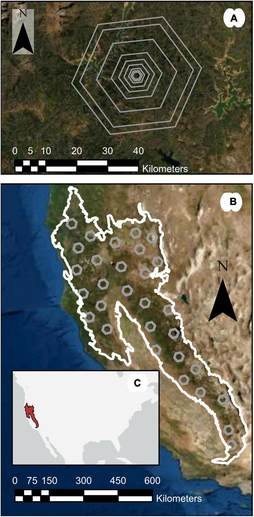
Study region map highlighting (A) nested hexagonal areas of interest, (B) 1,000,000-ha subregions within M261, and (C) an inset showing the study region location in the United States.
In addition to the environmental and ecological heterogeneity in forest landscapes within M261, tracking carbon emissions and sequestration has been of major interest in California, United States. Federal, state, and municipal governments leverage numerous mitigation strategies for emissions reductions and sequestration improvements, such as California’s forest offset program (Anderson et al., 2017; Cameron et al., 2017). These types of strategies require reliable information on forest carbon pools at a variety of scales, from all California forest lands down to individual property owners or management units. This study region (M261; Figure 1) and others would benefit greatly from an improved capacity to produce carbon pool estimates at a variety of scales as well as guidance with respect to appropriate use of NFI data provided by FIA.
Forest Inventory and Analysis Data
The FIA program is the NFI for the United States and provides a field-based assessment of forest conditions on a uniform triangular grid represented by a hexagonal lattice (one plot per 2,428-ha hexagon) across all lands regardless of ownership (i.e., non-private and private lands) in the United States (Bechtold and Patterson(eds), 2005). Through its design, the FIA plot network is well-suited for analyzing and quantifying forest conditions (e.g., volume, biomass, and carbon) at varying scales over time as the data provides a basis for unbiased estimates of forest conditions in a consistent and timely fashion (Glenn et al., 2015). As determined by aerial photography and other remote sensing, FIA locates a single plot in each 2,428-ha hexagon—either by random or collocated with a preexisting plot (Bechtold and Patterson(eds), 2005), but measures only those plots located on forestlands. On forestlands (i.e., land at least 0.4 ha in size that is at least 10% stocked with trees or formerly having such tree cover and not currently developed for a non-forest land use), field crews visit permanent ground plots and measure a suite of forest and tree variables, including tree species and diameter at breast height (dbh; 1.37 m). Plots consist four sets of nested subplots in a triangular arrangement, with trees 2.5–12.7 cm dbh measured on 2.07-m fixed radius subplots within larger 7.32-m fixed radius subplots used for trees at least 12.7 cm dbh. Therefore, field data are, at their most basic, measurements of tree species, size, and mortality status with associated scaling factors depending on size of the tree and the plot design described above. Additional measurements on FIA plots are plentiful (e.g., seedling counts, tree mortality agents, etc.), but are not used in the current study and are not discussed further.
Individual tree measurements were used to calculate ecosystem- or stand-level statistics, such as tree density, tree basal area, and species diversity. For this study, plot-level ALC was estimated using these tree diameter and species data by applying the Component Ratio Method (Jenkins et al., 2003; Woodall et al., 2011). We used tree measurements from 2014 to 2018 to represent the most recent forest conditions in the study area. While ALC estimates are themselves based on models and thus include error (Clough et al., 2016), we treat these as observations for the purposes of SAE in this study (sensuWilson et al., 2013).
Auxiliary Data
To support the generation of raster maps of imputed plots for the study area by assigning a set of k plots to pixels based on their proximity in feature space (e.g., Ohmann and Gregory, 2002), we identified and developed a suite of auxiliary variables (Figure 2). Predictive features, or auxiliary variables, were derived from a digital elevation model (DEM), climate data, and satellite imagery, then resampled to 30-m pixel resolution. Elevation, along with its derivatives, from the 1 arc-second DEM of the National Elevation Dataset (Gesch et al., 2002) formed the set of topographic features used. Topographic derivatives included slope, compound topographic index (Beven and Kirkby, 1979), and potential annual direct incident radiation (McCune and Keon, 2002). Climate variables, derived from the Daymet Version 3 (Thornton et al., 1997, 2016) 1-km gridded monthly summaries, included mean annual growing degree days and mean annual precipitation over the nearly 40-year record. The reflectance bands for each Landsat 8 OLI collection 1 scene collected during 2014–2018 were transformed to the Tasseled Cap (TC) components of brightness, greenness, and wetness (Kauth and Thomas, 1976; Baig et al., 2014). Harmonic regression, based on a 3rd-order Fourier series (Wilson et al., 2018), was employed to characterize the mean shape of the spectro-temporal profile for each pixel and TC component over the 5-year period. A 3rd-order Fourier series requires 7 model coefficients: one for the fundamental frequency, as well as a pair for each of the three harmonics (i.e., comprised of a sine and cosine term). Given that a series was fitted to each of the three TC profiles, a total of 21 model coefficients were estimated.
FIGURE 2
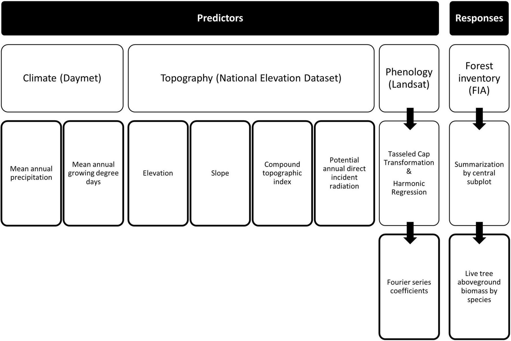
Summarization of the source and generation of predictor (auxiliary) and response (forest inventory) variables used in the development of kNN mapping of ALC.
Generating Tree Aboveground Live Carbon Estimates
Central to this manuscript is the comparison of multiple estimation techniques for areas of different sizes in terms of ALC mean and variance estimates. For this study, we examine the Horvitz-Thompson estimator as an example of traditional design-based estimation, GREG as an example of model-assisted estimation, and a synthetic estimator based on the k-nearest neighbors algorithm as an example of model-based estimation.
Horvitz-Thompson Estimator
Horvitz and Thompson (1952) developed an estimator that provides a general framework for direct estimation under multiple sample designs, whether or not auxiliary variables are available. The Horvitz-Thompson (HT) estimator for the population total Y is:
where, for the ith unit in a population of size N, Ii is a random variable that indicates whether or not the unit is in the sample, di is the unit’s design weight, and yi is the observation of the variable of interest for the unit. The design weight of a unit is the inverse of its probability of inclusion in the sample, πi, or di = 1. The inclusion probabilities are determined by the sample design, which defines whether or not the sample units are to be drawn, for example, from a simple random sample (SRS), systematic sample, or cluster sample. Yates and Grundy (1953) developed an estimator of the variance of the HT estimator,
where πij is the joint inclusion probability of units i and j.
Generalized Regression Estimator
One approach to estimation when auxiliary variables are available is to use a model-assisted estimator. One example is known as the calibration estimator, or the generalized regression (GREG) estimator (Deville and Särndal, 1992). The GREG estimator is a generalization of a class of estimators, such as the ratio and regression estimators, that use values of one or more auxiliary variables for all population units with an assisting model to calibrate the direct estimator. It still uses the design weights and is therefore fundamentally design-based. As described in Rao (2011), suppose that the parametric superpopulation model that describes the relationship between unit-level observations of the variable of interest and the auxiliary variables is,
where β are the model parameters, xi are the auxiliary data, and εi is the model error. In the current study, we used the predictions from a non-parametric kNN model to replace the term (see section Synthetic k-Nearest Neighbors Estimator). The errors are assumed to be uncorrelated with mean of zero and variance proportional to a known constant qi.
The GREG estimator of the population total Y is given by,
where X are the known population totals of the auxiliary variables and and are the corresponding estimated values for the variable of interest and auxiliary variables using the sampled units and their design weights. The variance is calculated as the Yates-Grundy variance, based on the model residuals. The working model used with the GREG estimator does not need to be a parametric linear model, and could instead be non-linear or, as in our study using the kNN algorithm, a non-parametric model.
Synthetic k-Nearest Neighbors Estimator
The model used as the foundation of our synthetic estimator and required as the auxiliary data for our GREG estimator (the β′X term) was based on the kNN algorithm (Fix and Hodges, Jr., 1952). The kNN imputation approach has been used extensively as a flexible, multivariate, and non-parametric method for forest attribute mapping (e.g., Ohmann and Gregory, 2002; Tomppo et al., 2008; Eskelson et al., 2009; McRoberts et al., 2011; Wilson et al., 2013). Here, we briefly describe the development of raster maps of imputed plots based on kNN as well as the SK used for generating areal estimates for the mean and variance of forest attributes. For mapping ALC in our study area, the kNN algorithm was used to impute ALC data to individual pixels where no tree measurements were taken based on their similarity to forest inventory plots with relation to some set of predictors (e.g., Figure 3). As the non-parametric kNN model was fit using the FIA sample for the entire study region M261 and then used to make predictions for all population units within several domains of the study region, it forms the basis for a synthetic estimate of ALC. While the kNN estimator is likely nearly, but not exactly, unbiased across all units in the sample (sensuMcRoberts et al., 2007; Magnussen et al., 2009), there is no guarantee this holds for a subsample, or any smaller domains.
FIGURE 3
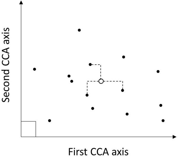
Conceptual diagram highlighting the kNN imputation process for a simple case with two metrics (CCA axes) defining the feature space. After the CCA modeling (solid circles) are located in the feature space, then a pixel to be imputed (open circle) is placed in that space based on the auxiliary data (geospatial predictors). Distances from the focal pixel to all plots in the feature space are calculated and the k nearest neighbors are identified by minimizing those distances (indicated by dashed lines). Each of those nearest neighbors was imputed back to the pixel to populate a multiband raster, with the mean ALC for neighbors across bands being the predicted ALC for the pixel.
An ecological ordination of tree species found in the ecological province was conducted using a canonical correspondence analysis (CCA) model (ter Braak, 1986). The set of 27 predictor variables described above used were the four topographic variables (slope, compound topographic index, and potential annual direct radiation), two climate variables, and 21 Fourier series coefficients associated with each pixel at the location of the plots measured during 2014–2018. The response variables used were live tree aboveground biomass per hectare by species for trees located on the central 7.32-m fixed radius subplot of the plots (Figure 2), to better match the pixel resolution of the predictor variables. There were 2,251 plots with live trees on forest conditions used to fit the CCA model.
The fitted CCA model coefficients formed the feature space for measuring proximity between each pixel and the set of measured plots (Figure 3; Ohmann and Gregory, 2002). All 27 orthogonal canonical variates of the CCA model were used with the kNN algorithm. Because the CCA model generates orthogonal axes, this approach avoids multicollinearity when assigning nearest neighbors based on the resulting feature space. There were 3,631 plot locations with a complete record of both predictor and response variables used in the imputation for M261, with non-forest conditions assigned a value of 0 for forest condition and tree variables. The value of k used for kNN regression, with predicted values being the unweighted mean of the k-nearest plots, excluding the nearest plot using the Manhattan distance metric, was selected to minimize mean squared error of predicted total live tree aboveground biomass. The optimal value of k for province M261 was 28.
To generate model-based mean and variance estimates for ALC based on the maps of nearest neighbors, we applied an areal estimation technique for kNN imputation (McRoberts et al., 2007; McRoberts, 2012), and our SK. For an AOI, the mean ALC was calculated as the mean pixel-level ALC across all forested pixels and the 28 nearest neighbors for each pixel, excluding the nearest plot. Variance estimation incorporated pixel-level variance in ALC across the 28 nearest neighbors as well as covariance between pixel pairs within an AOI. The covariance between any two pixels depends on the standard deviation in ALC across neighbors for each pixel and the number of plots shared by the two pixels within the list of the k = 28 nearest neighbors. Thus, the SK estimator generates model-based mean and variance estimates for ALC, or any other forest attribute of interest for which plot data are available.
Because imputed maps were based on plots that were visited in the field (i.e., forestlands) and we wished to avoid extrapolating beyond the scope of our input data, we used a map of forest type groups (Wilson, 2021) to mask out non-forest lands. As a result, we assume that ALC = 0 for non-forest lands. We also apply the SK estimator only for forestlands, meaning that mean and variance in ALC is for forestlands only. To generate mean ALC for all lands, we multiplied the mean ALC from the SK estimator with the proportion of pixels within an AOI that were forested. Because we assume that ALC = 0 for non-forest lands and is thus not a random variable, variance in ALC for all lands is equal to variance in ALC for forestlands.
For this study, we implemented the SK estimator using R and ArcGIS Pro. Our implementation of the SK estimator utilized an R script embedded within an ArcGIS Pro Model Builder Toolbox. Manipulation of spatial data was handled within ArcGIS Pro 2.6 and mean and variance calculations were processed in R (4.0.2; R Core Team, 2020) within ArcGIS Pro using the arcgisbindings package (version 1.0.1.244; Esri., 2021). ArcGIS Pro required Spatial Analyst and the following R packages: doParallel (version 1.0.16; Microsoft Corporation, and Weston, 2020), raster (version 3.4-5; Hijmans, 2020), rgdal (version 1.5-23; Bivand et al., 2021), rgeos (version 0.5-5; Bivand and Rundel, 2020), and snow (version 0.4-3; Tierney et al., 2018). To accelerate processing time, we adopted a subsampling approach for pixels within an AOI, avoiding the need to assess all pairwise comparisons of individual pixels (McRoberts et al., 2007). An example R script upon which our ArcGIS Pro workflow is based can be found in Supplementary Material 1.
To determine whether variance estimates with the subsampling approach converge on the estimate based on all pixels (i.e., stability of variance estimator), we generated five replicates for each of the 30 subregions of randomly selected pixels for sample proportions from 0.01 to 0.30 and AOI areas of 1,000, 5,000, and 10,000 ha. Initial testing on a high-end workstation indicated that computation time scaled with the square of the number of pixels. Given that constraint, we limited the generation of replicates to intervals of 0.01 for sample proportion between 0.01 and 0.15, but also generated replicates at sample proportions of 0.20, 0.25, and 0.30. The upper value of 0.30 was selected as it was roughly double the recommendation from a previous study (McRoberts et al., 2007). Thus, we attempted to balance reasonable computation time with appropriate coverage of lesser sample proportions which we assumed would be less stable. We then estimated variance for each replicate, sample proportion, and area combination and calculated the percent difference between that estimate and the estimate derived from the one generated when using all pixels in an AOI.
To identify the proportion of pixels that must be subsampled to generate SK variance estimates that converge on the estimate using all pixels within an AOI (i.e., a stable variance estimate), we used ordinary least squares regression (lm function; R Core Team, 2020) to fit a regression model for the absolute value of the proportional difference between sample and full variance SK estimates as a function of forest area within each AOI and proportion of pixels in the AOI sampled to generate variance estimates. Given that we were generating ALC estimates for forest lands, rather than all lands, we used forest area instead of AOI area to reflect the total number of pixels, and thus the amount of information, being used by the SK variance estimator. Additionally, forest area accounts for both AOI area as well as forest dominance (proportion of AOI that was forested). We included proportion of AOI being subsampled to represent the influence of the subsampling procedure. Data exploration indicated that the greatest predictive power for the regression model was achieved when log-transforming both response and predictor variables. We compared regression models with differing combinations of main effects (P and F) using AIC, selecting the model that minimized AIC as the best.
To solve for the proportion of pixels to sample P for values of forest area F in order to generate variance estimates within 1% of the estimate using all pixels in an AOI (Y = 0.01), we reorganize the regression equation as
When P > 1, we set P = 1 as this indicates a need to use all pixels in an AOI. Note that forest area is the product of AOI area and forest dominance, such that for any AOI area, the proportion of pixels to be sampled depended on the forest dominance in the AOI.
Comparisons of Tree Aboveground Live Carbon Estimates
To compare ALC estimates generated by the differing approaches across scales, we first defined areas of interest (AOI) across the study region in order to represent a diverse suite of forest conditions (Figure 1A). Across M261, we created 30 1,000,000-ha hexagons as subregions covering 500,000–1,000,000 ha each. For each subregion, we selected the 648 km2 Environmental Monitoring and Assessment (EMAP) hexagons (White et al., 1992) overlapping the centroid of the subregion, resulting in 30 hexagons 64,800 ha in size across the study region M261 (Figure 1B). For FIA-based forest attribute estimation, the EMAP hexagons have been identified as providing a balance between fine spatial scale and sufficient numbers of plots to support design-based inference (Woodall et al., 2006; Menlove and Healey, 2020). We then generated hexagons at eight additional scales, centered on the same centroids: 50,000, 25,000, 10,000, 5,000, 2,500, 1,000, 500 ha, and 250 ha. These hexagons were the estimation units for this study.
We compared mean and variance estimates from each of the different methods described above (HT, GREG, and SK) only for the 10,000, 25,000, 50,000, and 64,800-ha AOIs. We compared results from the GREG and SK estimators with the HT estimator results using simple linear regression in order to roughly assess uncertainties in model-assisted and model-based estimators relative to design-based estimators. For each AOI at each scale, we also computed the relative efficiency (RE) of the SK and GREG estimators relative to the HT estimator and to each other, which is simply the ratio of the variances being compared. Two versions of the SK estimator were used for these comparisons. Unadjusted SK is the usual synthetic estimator that, by assuming the modeled relationship between predictor and response variables developed for M261 holds for all domains within it, also assumes unbiasedness for SAE. Adjusted SK uses the design-weighted estimate of the bias provided by the sample to calculate mean square error, where MSE = variance + bias2. Under most SAE scenarios, this adjustment would not be possible because of small sample sizes.
The SK estimator was applied to all scales described above, though larger areas can require substantial processing time. It should be noted that there are many users interested in estimating means and variances for forest attributes for areas that are much smaller (<10,000 ha). Therefore, we present variance estimates for smaller areas to quantify estimate variance for the SK estimator at scales relevant to forest managers. To examine the variance of ALC estimates across a gradient of AOI area (250–64,800 ha) for the SK estimator, we developed linear mixed effect regressions of the log relative standard error (% of mean ALC estimate) as a function of log forest area, forest dominance, and a random effect for the 1,000,000-ha subregion. Forest dominance was calculated as the proportion of area in an AOI that was forested. We used all the estimates across scales (250–64,800 ha) for the 30 subregions as inputs. We then used the lme function in R (nlme package version 3.1-140; Pinheiro et al., 2019) to fit a model for log relative standard error in the ALC estimates as
where yij was the log relative standard error for AOI i in subregion j, γ0, γ1, and γ2 were regression parameters, Aij was the forest area (ha) in AOI i in subregion j, Dij was the forest dominance (unitless) in AOI i in subregion j, σ2 was the process variance for the regression, αj was the random effect for subregion j, and τ2 was the variance for the random effects. We fit two additional linear regression models, one with forest area Aij only and one with forest area Aij and forest dominance Dij, in order to examine the explanatory power of each component of the model describing the coefficient of variation.
Results
Small Area Estimate Convergence
We tested the stability of the SK variance estimator as a function of the proportion of pixels sampled. We found that increasing the proportion of pixels sampled quickly led to convergence in variance estimates, supporting the use of only a subset of pixels with an AOI (Figure 4). We found that generating variance estimates within 1% of the estimate based on all pixels depended on several factors, including AOI area and proportion of pixels being sampled. For 10,000-ha AOIs, sampling 7% of pixels resulted in most variance estimates being within 1% of the estimate using all pixels, whereas 15% were required to ensure that most estimates were within 0.5%. Proportion of pixels sampled needed to increase for smaller areas to achieve the same convergence in variance estimates, with 5,000 ha AOIs requiring 14% and 1,000 ha AOIs requiring 30% of pixels sampled for most estimates to converge within 1%.
FIGURE 4
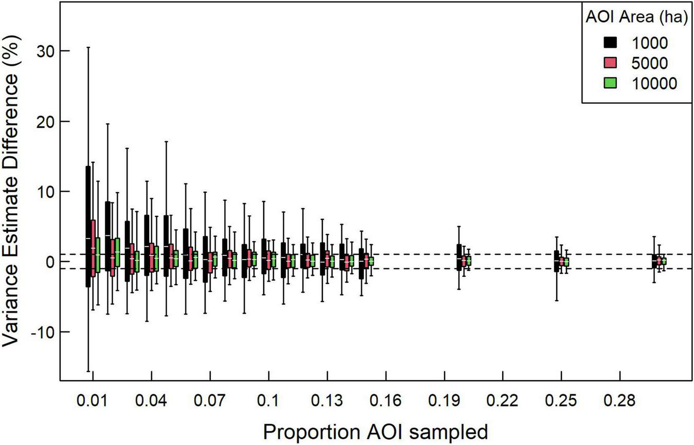
Percent difference between AOI variance estimates based on a sample of pixels vs. using all pixels for AOIs of differing sizes. In this case, we examined 30 1,000, 2,500, and 10,000-ha AOIs distributed across the study region, each with five replicates. White horizontal lines indicate median, boxes indicate 50% intervals, and whiskers indicate 90% intervals. Dashed horizontal lines demarcate –1 and 1% differences.
Our regression analysis examining the stability of variance estimates indicated that the best model for log absolute value of the proportional difference between sample and full variance estimates Y explained 33.5% of the variation and included an intercept (β0 = −1.868 ± 0.088 SE), log forest area F (β1 = −0.516 ± 0.010 SE), and log proportion pixels sampled P (β2 = −0.576 ± 0.015 SE).
Predicted proportion sampled increased as AOI area and forest dominance within the AOI decreased, indicating that the stability of the variance estimate depends on the number of pixels being considered. For the purposes of the rest of this study, we set the proportion of pixels sampled for estimating variance using the SK estimator to the values predicted by the 25% forest cover scenario (gray diamonds in Figure 5) to increase the likelihood of estimate convergence. Thus, to generate variance estimates using the SK estimator for 250, 500, 1,000, 2,500, 5,000, 10,000, 25,000, 50,000, and 64,800-ha AOIs, we used 1.00, 1.00, 0.82, 0.36, 0.19, 0.10, 0.05, 0.02, and 0.02 for proportion of pixels sampled.
FIGURE 5
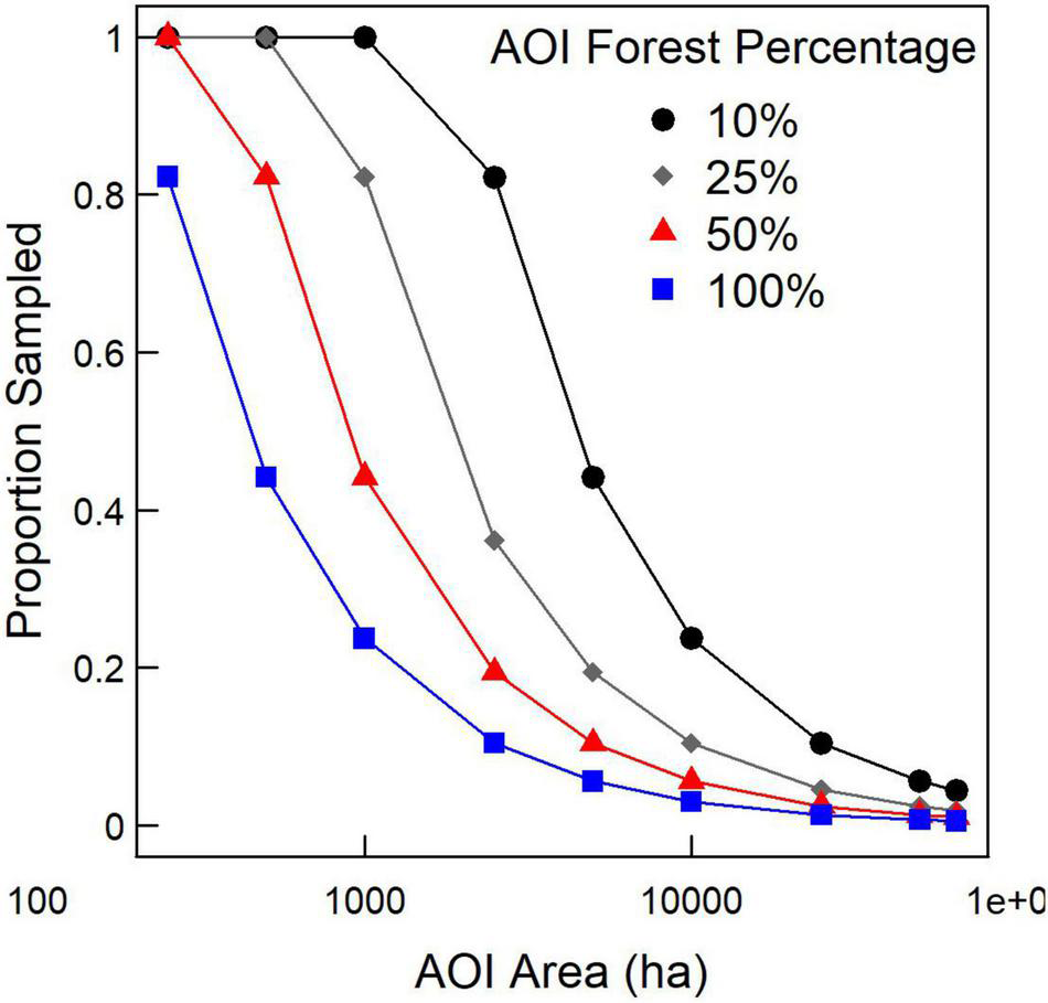
Proportion of pixels sampled for AOIs of differing sizes and forest extent to, on average, generate variance estimates within 1% of the variance estimate using all pixels.
Comparing Estimation Methods Across Scales
Mean ALC estimates based on GREG generally agreed with HT estimates, though that agreement decreased as AOI area decreased (Table 1). Regressions of GREG and HT mean ALC estimates across AOIs showed that slopes decreased from 1.010 to 0.818 and R2 decreased from 0.972 to 0.805 as AOI area decreased from 64,800 to 10,000 ha. The regression intercept also decreased as AOI area decreased. Relative standard errors increased from 16 to 31%, while the RE of GREG vs. HT estimators increased from 1.45 to 1.54 as AOI area decreased.
TABLE 1
| Area (ha) | m | b/ | R2 | RSE | RE (HT) |
| 10,000 | 0.818 | 0.215 | 0.805 | 30.977 | 1.542 |
| 25,000 | 0.954 | 0.113 | 0.928 | 24.566 | 1.556 |
| 50,000 | 0.991 | 0.093 | 0.946 | 21.234 | 1.406 |
| 64,800 | 1.010 | 0.062 | 0.972 | 16.148 | 1.450 |
Regression results (y = mx+b) of the scatterplot of GREG (x) vs. HT (y) estimates across spatial scales, along with median relative standard error (% of estimate) and median RE of the GREG vs. HT estimator.
Comparisons of the SK estimator with HT and GREG estimators indicated a more complex story regarding estimator performance (Table 2). Like GREG, regression of SK and HT mean ALC estimates indicated decreasing agreement with decreasing AOI area, with R2 ranging from 0.920 to 0.758 for 64,800 and 10,000 ha areas, respectively. Slopes from the regression were relatively constant (0.992–1.026) for scales greater than or equal to 25,000 ha, but decreased to 0.905 for 10,000 ha AOIs, while intercepts increased as AOI area decreased. Relative standard errors for unadjusted SK were smaller than other estimators (7.8–8.4%), resulting in RE compared to HT of 4.5–16.8. However, the unadjusted SK estimator RE values do not account for potential biases inherent in the synthetic approach. When we accounted for bias, using the design-weighted estimate of bias, relative root mean square error of adjusted SK increased from 24 to 33% and RE compared to HT increased from 0.649 to 2.269 as AOI area decreased from 64,800 to 10,000 ha. Similarly, adjusted SK estimator RE compared to GREG increased from 0.496 to 1.263 as AOI area decreased from 64,800 to 10,000 ha.
TABLE 2
| Unadjusted synthetic | Adjusted synthetic | ||||||||
| Area (ha) | m | b/ | R2 | RSE | RE (HT) | RE (GREG) | RRMSE | RE (HT) | RE (GREG) |
| 10,000 | 0.905 | 0.073 | 0.758 | 7.880 | 16.843 | 11.853 | 33.284 | 2.269 | 1.263 |
| 25,000 | 1.024 | −0.002 | 0.874 | 8.185 | 11.088 | 6.450 | 24.496 | 1.263 | 1.226 |
| 50,000 | 1.026 | −0.037 | 0.897 | 8.356 | 7.079 | 5.149 | 25.023 | 0.904 | 0.681 |
| 64,800 | 0.992 | −0.047 | 0.920 | 8.383 | 4.542 | 3.536 | 24.033 | 0.649 | 0.496 |
Regression results (y = mx+b) of the scatterplot of the unadjusted synthetic (x) vs. HT (y) estimates across spatial scales, along with median relative standard error (% of estimate) and median relative efficiency of the synthetic vs. HT and GREG estimators.
Adjusted synthetic results are based on root mean square error, including the HT estimate of bias.
Across subregions, linear mixed effects modeling indicated that the relative standard error for ALC from the SK estimator decreased with forest area and forest dominance within an AOI (Table 3 and Figure 6A). The linear mixed effects model including log forest area, log forest dominance, and a random effect for subregion explained 93% of the variation in the log coefficient of variation, whereas models without random effects or without random effects and forest dominance explained 59 and 39% of the variation, respectively. Mapping random effects indicated that coefficient of variation tended to be lesser in the northwestern, greater in the northeastern, and more variable in the southern portion of the study area (Figure 6B).
TABLE 3
| Model | β0 | β1 | β2 | Residual standard error | Random effect variance (τ2) | R2 |
| Forest area | −1.817 (0.140) | −0.104 (0.008) | 0.270 | 0.39 | ||
| Forest area and dominance | −1.551 (0.058) | −0.095 (0.007) | −0.537 (0.047) | 0.222 | 0.59 | |
| Forest area, dominance, and subregion random effect | −1.803 (0.062) | −0.088 (0.003) | −0.223 (0.048) | 0.096 | 0.050 | 0.93 |
Fixed effect and mixed effect linear regression results for predicting the log coefficient of variation in tree aboveground live carbon as a function of area, dominance, and subregion.
FIGURE 6
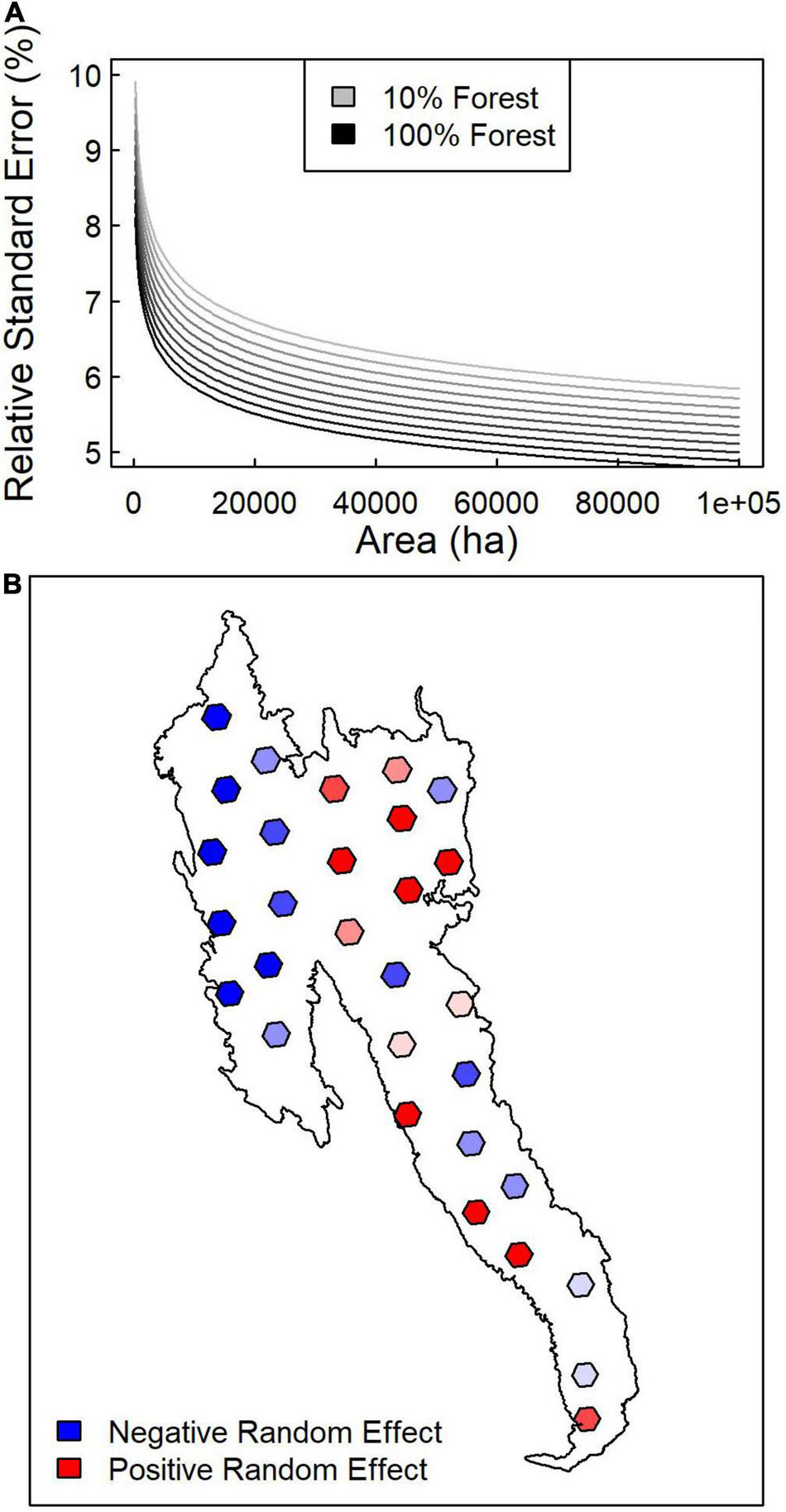
Mixed effects regression results of relative standard error as a function of scale and landscape. (A) Mean predictions of coefficient of variation based on forested area and forest dominance (percent of AOI that is forested). (B) Spatial distribution of random effects across study area.
Discussion
Comparing Estimators (10,000–64,800 ha)
Augmenting NFI data with auxiliary data using either model-assisted or model-based estimation facilitates SAE, but our results emphasize that the appropriate estimation procedure depends upon the area of an AOI, and thus the sample of plots, being considered. In our study, 25,000 ha was the nominal scale below which one would consider changing from the GREG to the adjusted SK estimator, or vice versa: RE for GREG was greatest among estimators tested for areas larger than 25,000 ha and RE for adjusted SK was greatest for areas less than or equal to 25,000 ha (Tables 1, 2). In the case of the FIA data used in this study, 25,000 ha roughly equates to 10 plots whereas the commonly used EMAP hexagons (64,800 ha) would generally contain 27 plots. Even at the 64,800-ha scale, the GREG estimator RE compared to HT was greater than one, indicating that GREG estimators should be preferred given sufficient plot support in an AOI.
Our results highlight a fundamental limitation of the unadjusted SK estimator examined: the lack of appropriate accounting of bias. The synthetic estimator used in this study assumes unbiasedness in pixel predictions (McRoberts et al., 2007). Given that regression slopes close to one and intercepts close to zero highlight agreement, SK mean ALC estimates did not exhibit major systematic lack of fit, but R2-values were less than those reported for GREG (Tables 1, 2). This increased error in mean predictions was not reflected in the unadjusted SK variance estimates, which were considerably smaller than GREG or HT variance estimates. Previous examinations of the kNN synthetic estimator used in this study indicated that kNN using NFI data can be unbiased with respect to the sampling aspects of the estimator, but not necessarily in terms of the bias associated with model mis-specification (McRoberts et al., 2007; Magnussen et al., 2009; McRoberts, 2012). Such bias, for example, motivates the use of empirical best linear unbiased prediction (such as a Fay-Herriot model) or composite estimators that minimize MSE by finding the optimal balance between the low variance of a synthetic estimator and the unbiasedness of a direct estimator (such as a James-Stein estimator) (Breidenbach and Astrup, 2012; Rao and Molina, 2015; Mauro et al., 2017; Coulston et al., 2021). Thus, while the unadjusted SK estimator can produce variance estimates far smaller than other methods (McRoberts et al., 2007; Breidenbach et al., 2010), they reflect only model variance, not bias. While model-based variance estimates can be useful for many applications, focusing primarily on variance estimates without accounting for model bias leads to an overly optimistic view of uncertainty.
Still, it is interesting that the adjusted SK estimator RE compared to HT and GREG support the use of synthetic estimators at smaller scales where few plots were available. One might speculate that improving model fit or accounting for biases among AOIs would improve relative efficiencies and increase the nominal area for which one would select SK vs. GREG estimators. Our results imply that development or application of model-based SAE should incorporate an assessment against GREG at the scales relevant to the individual study to determine whether estimates are improved in a practical sense.
k-Nearest Neighbors Variance Estimates (250–64,800 ha)
In our study, the SK variance estimates relative to the mean ALC was predictable (Table 3), indicating that land cover and AOI area determine the precision of estimates derived from the SK estimator. Relative standard error for ALC depended almost entirely on forest area within the AOI, forest dominance, and biogeographic variation at the scale of our 1,000,000-ha subregions. Across forest dominance gradients, average predicted relative standard errors ranged between 0.05 and 0.07 for the largest forest areas (64,800 ha) and 0.08–0.11 for the smallest forest areas (250 ha) (Figure 6A). However, geographic variation in random effects imply that broad-scale variation in forest conditions explains roughly one third of the relative standard error (Figure 6B). This result is consistent with our previous examination of lidar-based vs. Landsat-based maps of forest biomass which highlighted increasing differences and decreasing correlation between the two products as one shifted from coniferous to mixed broadleaf-coniferous forest landscapes (Bell et al., 2018). It has also been shown that stratification by forest type prior to lidar-based modeling improves biomass and carbon mapping (Swatantran et al., 2011; Chen et al., 2012), implying that variation in forest composition and structure influences prediction and estimation approaches.
Our results support the general application of a subsampling approach in this SK estimator using kNN, but the degree of subsampling depends on the area of the AOI and the amount of forest located within it. Variance estimates based on a subsample of pixels converged on the estimate using all pixels as AOI area increased (Figure 4), but that convergence appeared to be delayed with lesser forest dominance (Figure 5). The convergence still appears to be quite variable (R2 = 0.25), indicating other factors may determine convergence for any given AOI. Based on this uncertainty in convergence, we recommend a relatively conservative approach to selecting proportion of pixels to sample. In our case, we assumed that forest dominance (proportion of pixels forested in AOI) was 0.25. Given that our results for 10,000 ha AOIs were similar to a previous study in Minnesota (15% sampling threshold; McRoberts et al., 2007) and are relatively consistent regardless of the area forested in within the AOI (134–9,740 ha), these results may be broadly applicable across landscapes. Still, further application of this method would necessitate examination of convergence as a function of other biophysical factors, such as forest type group, so that users could easily identify the appropriate sub-sampling to apply for stable variance estimation.
Conclusion
Forest managers increasingly rely upon spatially explicit, mapped forest attribute data as central source of information for decision-making, but assessments of uncertainty provide a much needed characterization of variance and bias in estimates of stand-, landscape-, and region-level forest attribute estimates (Tomppo et al., 2008; McRoberts, 2012). Though the choice of inferential mode, from design-based to model-based, will always depend on the question being asked (Ståhl et al., 2016), the scale of inference and characteristics of forest ecosystems appear to play a dominant role in estimate uncertainty. This study (Table 3 and Figure 6) and others (e.g., Bell et al., 2015, 2018) show that spatial variation in estimated variance may be predictable as a function of biophysical characteristics of the ecosystems being studied. Advances in model-based estimation that properly account for bias in estimation error (e.g., Mauro et al., 2017; Coulston et al., 2021) could extend the scale at which these approaches outperform model-assisted estimation (e.g., > 25,000 ha). Such advances could be integrated into estimation procedures to guide the selection of estimators to fully characterize both model precision and bias, both of which impact the utility of estimates for users.
We suggest that an improved understanding of synthetic estimator uncertainty across a diversity of forest landscapes could form the basis for a simple, yet transparent workflow for forest attribute estimation. That platform could open the use of regional or national forest inventory data to a broader community of users. These improvements should, in part, aim to incorporate a proper accounting of prediction bias in model-based estimation for small areas. Furthermore, the identification of nominal scales at which users should generally switch from one estimation technique (e.g., GREG) to another (e.g., synthetic) could be incorporated into an integrated approach that guides users on the appropriate estimator to use at the scale of their AOI. However, both producers and users of estimates should bear in mind potential biases in predictions that, in the case of the SK, result in overly precise (i.e., lesser variance) estimates of forest attributes. By exploring multiple scales of application for an SAE procedure applied to NFI data regarding carbon pools, this research lays the groundwork for a multi-scale estimation framework in a simple and transparent manner that guides users in developing defensible estimates and educates users on the limits of inference at a variety of spatial scales.
Author Disclaimer
The findings and conclusions in this report are those of the author(s) and do not necessarily represent the views of the USDA Forest Service.
Publisher’s Note
All claims expressed in this article are solely those of the authors and do not necessarily represent those of their affiliated organizations, or those of the publisher, the editors and the reviewers. Any product that may be evaluated in this article, or claim that may be made by its manufacturer, is not guaranteed or endorsed by the publisher.
Statements
Data availability statement
Publicly available datasets were analyzed in this study. This data can be found here: https://www.fia.fs.fed.us/.
Author contributions
DB led all components of this research. DB, BW, and CW developed and carried out the analyses, including the generation of figures and tables and wrote the majority of the manuscript. All authors contributed to the development of the research questions and the kNN-SAE approach and provided comments and edits on the final version of the manuscript.
Funding
This research was funded by the USDA Forest Service, including the collection of FIA plot data used in this study.
Acknowledgments
We would like to thank Gregory Brunner, Peter Eredics, Andrew Leason, Robert Richard, and John Steffenson for their contributions to the development of kNN mapping for CONUS.
Conflict of interest
The authors declare that the research was conducted in the absence of any commercial or financial relationships that could be construed as a potential conflict of interest.
Supplementary material
The Supplementary Material for this article can be found online at: https://www.frontiersin.org/articles/10.3389/ffgc.2022.763422/full#supplementary-material
References
1
AndersonC. M.FieldsC. B.MachK. J. (2017). Forest offsets partner climate-change mitigation with conservation.Front. Ecol. Environ.15:359–365. 10.1002/fee.1515
2
BaigM. H. A.ZhangL.ShuaiT.TongQ. (2014). Derivation of a tasselled cap transformation based on Landsat 8 at-satellite reflectance.Remote Sens. Lett.5423–431. 10.1080/2150704X.2014.915434
3
BechtoldW. A.PattersonP. L. (eds) (2005). The Enhanced Forest Inventory and Analysis Program - National Sampling Design and Estimation Procedures.Gen. Tech. Rep. SRS-80. Asheville, NC: U.S. Department of Agriculture, 85.
4
BellD. M.GregoryM. J.OhmannJ. L. (2015). Imputed forest structure uncertainty varies across elevational and longitudinal gradients in the western Cascade Mountains, Oregon, USA.For. Ecol. Manag.358154–164. 10.1016/j.foreco.2015.09.007
5
BellD. M.GregoryM. J.KaneV.KaneJ.KennedyR. E.RobertsH. M.et al (2018). Multiscale divergence between landsat- and lidar-based biomass mapping is related to regional variation in canopy cover and composition.Carbon Bal. Manag.13:15. 10.1186/s13021-018-0104-6
6
BeaudoinA.BernierP. Y.GuindonL.VillemaireP.GuoX. J.StinsonG.et al (2014). Mapping attributes of Canada’s forests at moderate resolution through kNN and MODIS imagery.Can. J. For. Res.44521–532. 10.1139/cjfr-2013-0401
7
BevenK. J.KirkbyM. J. (1979). A physically based, variable contributing area model of basin hydrology.Hydrol. Sci. J.2443–69. 10.1080/02626667909491834
8
BivandR.KeittT.RowlingsonB. (2021). rgdal: Bindings for the ‘Geospatial’ Data Abstraction Library. R Package Version 1.5-23. Available online at: https://CRAN.R-project.org/package=rgdal(accessed December 15, 2021).
9
BivandR.RundelC. (2020). rgeos: Interface to Geometry Engine - Open Source (‘GEOS’). R Package Version 0.5-5. Available online at: https://CRAN.R-project.org/package=rgeos(accessed December 15, 2021).
10
BreidenbachJ.AstrupR. (2012). Small area estimation of forest attributes in the Norwegian National forest inventory.Eur. J. For. Res.1311255–1267. 10.1007/s10342-012-0596-7
11
BreidenbachJ.NothdurftmA.KändlerG. (2010). Comparison of nearest neighbor approaches for small area estimation of tree species-specific forest inventory attributes in central Europe using airborne laser scanner data.Eur. J. For. Res.129833–846. 10.1007/s10342-010-0384-1
12
BrodieL. C.PalmerM. (2020). California’s Forest Resources, 2006-2015: Ten-Year Forest Inventory and Analysis Report.General Technical Report PNW-GTR-983. Portland, OR: USDA, Forest Service, Pacific Northwest Research Station, 60.
13
CameronD. R.MarvinD. C.RemucafJ. M.PasseroM. C. (2017). Ecosystem management and land conservation can substantially contribute to California’s climate mitigation goals.Proc. Natl. Acad. Sci. U.S.A.11412833–12838. 10.1073/pnas.1707811114
14
ChenQ.LaurinG. V.BattlesJ. J.SaahD. (2012). Integration of airborne lidar and vegetation types derived from aerial photography for mapping aboveground live biomass.Remote Sens. Environ.121108–117. 10.1016/j.rse.2012.01.021
15
ChenQ.McRobertsR. E.WangC.RadtkeP. J. (2016). Forest aboveground biomass mapping and estimation across multiple scales using model-based inference.Remote Sens. Environ.184350–360. 10.1016/j.rse.2016.07.023
16
ClelandD. T.AversP. E.McNabW. H.JensenM. E.BaileyR. G.KingT.et al (1997). “National hierarchical framework of ecological units,” in Ecosystem Management Applications for Sustainable Forest and Wildlife Resources, edsBoyceM. S.HaneyA. (New Haven, CT: Yale University Press), 181–200.
17
ClelandD. T.FreeoufJ. A.KeysJ. E.NowackiG. J.CarpenterC. A.McNabW. H. (2007). Ecological Subregions: Sections and Subsections for the Conterminous United States.General Technical Report WO-76D. Washington, DC: Washington Office, 76. 10.2737/WO-GTR-76D
18
CloughB. J.RussellM. B.DomkeG. M.WoodallC. W. (2016). Quantifying allometric model uncertainty for plot-level live tree biomass stocks with a data-driven, hierarchical framework.For. Ecol. Manag.372175–188. 10.1016/j.foreco.2016.04.001
19
CoulstonJ. W.GreenP. C.RadkeP. J.PrisleyS. P.BrooksE. B.ThomasV. A.et al (2021). Enhancing the precision of broad-scale forestland removals estimates with small area estimation techniques.Forestry94427–441. 10.1093/forestry/cpaa045
20
DavisR. J.OhmannJ. L.KennedyR. E.CohenW. B.GregoryM. J.YangZ.et al (2015). Northwest Forest Plan – The First 20 Years (1994-2013): Status and Trends of Late-Successional and Old-Growth Forests.PNW-GTR-911. Portland, OR: Pacific Northwest Research Station. 10.2737/PNW-GTR-911
21
DevilleJ.-C.SärndalC. E. (1992). Calibration estimators in survey sampling.J. Am. Stat. Assoc.87376–382. 10.1080/01621459.1992.10475217
22
DuL.ZhouT.ZouZ.ZhouX.HuangK.WuH. (2014). Mapping forest biomass using remote sensing and national forest inventory in China.Forests51267–1283. 10.3390/f5061267
23
EskelsonB. N. I.TemesgenH.LemayV.BarrettT. M.CrookstonN. L.HudakA. T. (2009). The roles of nearest neighbor methods in imputing missing data in forest inventory and monitoring databases.Scand. J. For. Res.24235–246. 10.1080/02827580902870490
24
Esri. (2021). arcgisbinding: Bindings for ArcGIS. R Package Version 1.0.1.244. Available online at: http://esri.com
25
FixE.HodgesJ. L.Jr. (1952). Discriminatory Analysis-Nonparametric Discrimination: Small Sample Performance.Berkeley, CA: California Univ Berkeley. 10.1037/e471672008-001
26
GeschD.OimoenM.GreenleeS.NelsonC.SteuckM.TylerD. (2002). The national elevation dataset. Photogramm. Eng. Remote Sensing68, 5–32.
27
GlennC. A.WaddellK. L.StantonS. M.KueglerO. (eds) (2015). California’s Forest Resources: Forest Inventory and Analysis, 2001–2010.Gen. Tech. Rep. PNW-GTR-913. Portland, OR: U.S. Department of Agriculture, 293.
28
GoerndtM. E.MonleonV. J.TemesgenH. (2012). Small-area estimation of county-level forest attributes using ground data and remote sensed auxiliary information.For. Sci.59536–548. 10.5849/forsci.12-073
29
HijmansR. J. (2020). raster: Geographic Data Analysis and Modeling. R Package Version 3.4-5. Available online at: https://CRAN.R-project.org/package=raster(accessed January 22, 2022).
30
HorvitzD. G.ThompsonD. J. (1952). A generalization of sampling without replacement from a finite universe.J. Am. Stat. Assoc.47663–685. 10.1080/01621459.1952.10483446
31
JenkinsJ. C.ChojnackyD. C.HeathL. S.BirdseyR. A. (2003). National scale biomass estimators for United States tree species.For. Sci.4912–35.
32
KauthR. J.ThomasG. S. (1976). “The tasselled cap–a graphic description of the spectral-temporal development of agricultural crops as seen by landsat,” in Proceedings, Symposium on Machine Processing of Remotely Sensed Data, West Lafayette, IN, 159.
33
ListerA. J.AndersenH.FrescinoT.GatziolisD.HealeyS.HeathL. S.et al (2020). Use of remote sensing data to improve efficiency of national forest inventories: a case study from the United States national forest inventory.Remote Sens.11:1364. 10.3390/f11121364
34
MagnussenS.McRobertsR. E.TomppoE. O. (2009). Model-based mean square error estimators for k-nearest neighbour predictions and applications using remotely sensed data for forest inventories.Remote Sens. Environ.113476–488. 10.1016/j.rse.2008.04.018
35
MauroF.MonleonV. J.TemesgenH.FordK. R. (2017). Analysis of area level and unit level models for small area estimation in forest inventories assisted with LiDAR auxiliary information.PLoS One12:e0189401. 10.1371/journal.pone.0189401
36
McConvilleK. S.MoisenG. G.FrescinoT. S. (2020). A tutorial on model-assisted estimation with application to forest inventory.Forests11:244. 10.3390/f11020244
37
McCuneB.KeonD. (2002). Equations for potential annual direct incident radiation and heat load.J. Veg. Sci.13603–606. 10.1111/j.1654-1103.2002.tb02087.x
38
McRobertsR. E.TomppoE. O. (2007). Remote sensing support for national forest inventories.Remote Sens. Environ.110412–419. 10.1016/j.rse.2006.09.034
39
McRobertsR. E.TomppoE. O.FinleyA. O.JuhaH. (2007). Estimating areal means and variances of forest attributes using the k-nearest neighbors technique and satellite imagery.Remote Sens. Environ.111466–480. 10.1016/j.rse.2007.04.002
40
McRobertsR. E.MagnussenS.TomppoE. O.ChiriciG. (2011). Parametric, bootstrap, and jackknife variance estimators for the k-nearest neighbors technique with illustrations using forest inventory and satellite image data.Remote Sens. Environ.1153165–3174. 10.1016/j.rse.2011.07.002
41
McRobertsR. E. (2012). Estimating forest attribute parameters for small areas using nearest neighbor techniques.For. Ecol. Manag.2723–12. 10.1016/j.foreco.2011.06.039
42
MenloveJ.HealeyS. P. (2020). A comprehensive forest biomass dataset for the USA allows customized validation of remotely sensed biomass estimates.Remote Sens.12:4141. 10.3390/rs12244141
43
Microsoft Corporation, WestonS. (2020). doParallel: Foreach Parallel Adaptor for the ‘Parallel’ Package. R Package Version 1.0.16. Available online at: https://CRAN.R-project.org/package=doParallel(accessed October 16, 2020).
44
NieM. (2018). The forest service’s 2012 planning rule and its implementation: federal advisory committee member perspectives.J. For.11765–71. 10.1093/jofore/fvy055
45
OhmannJ. L.GregoryM. J. (2002). Predictive mapping of forest composition and structure with direct gradient analysis and nearest-neighbor imputation in coastal Oregon, USA.Can. J. For. Res.32725–741. 10.1139/x02-011
46
OhmannJ. L.GregoryM. J.RobertsH. M.CohenW. B.KennedyR. E.YangZ. (2012). Mapping change of older forest with nearest neighbor imputation and landsat time-series.For. Ecol. Manag.27213–25. 10.1016/j.foreco.2011.09.021
47
PinheiroJ.BatesD.DebRoyS.SarkarD.R Core Team. (2019). _nlme: Linear and Nonlinear Mixed Effects Models. R Package Version 3.1-140. Available online at: https://CRAN.R-project.org/package=nlme(accessed January 13, 2022).
48
R Core Team (2020). R: A Language and Environment for Statistical Computing, Version 4.0.2.Vienna: R Foundation for Statistical Computing.
49
RaoJ. N. K. (2011). Impact of frequentist and Bayesian methods on survey sampling practice: a selective appraisal.Stat. Sci.26240–256. 10.1214/10-STS346
50
RaoJ. N. K.MolinaI. (2015). Small Area Estimation, 2nd Edn. Hoboken, NJ: John Wiley & Sons, Inc, 441. 10.1002/9781118735855
51
SaatchiS. S.HarrisN. L.BrownS.LefskyM.MitchardE. T. A.AlasS.et al (2011). Benchmark map of forest carbon stocks in tropical regions across three continents.Proc. Natl. Acad. Sci. U.S.A.1089899–9904. 10.1073/pnas.1019576108
52
StåhlG.SaarelaS.SchenllS.HolmS.BreidenbachJ.HealeyS. P.et al (2016). Use of models in large-area forest surveys: comparing model-assisted, model-based and hybrid estimation.For. Ecosyst.3:5. 10.1186/s40663-016-0064-9
53
StankeH.FinleyA. O.WeedA. S.WaltersB. F.DomkeG. M. (2020). rFIA: an R package for estimation of forest attributes with the US forest inventory and analysis database.Environ. Model. Softw.127:104664. 10.1016/j.envsoft.2020.104664
54
SwatantranA.DubayahR.RobertsD.HoftonM.BlairJ. B. (2011). Mapping biomass and stress in the Sierra Nevada using lidar and hyperspectral data fusion.Remote Sens. Environ.1152917–2930. 10.1016/j.rse.2010.08.027
55
ter BraakC. J. F. (1986). Canonical correspondence analysis: a new eigenvector technique for multivariate direct gradient analysis.Ecology671167–1179. 10.2307/1938672
56
ThorntonP. E.RunningS. W.WhiteM. A. (1997). Generating surfaces of daily meteorological variables over large regions of complex terrain.J. Hydrol.190214–251. 10.1016/S0022-1694(96)03128-9
57
ThorntonP. E.ThorntonM. M.MayerB. W.WeiY.DevarakondaR.VoseR. S.et al (2016). Daymet: Daily Surface Weather Data on a 1-km Grid for North America, Version 3.Oak Ridge, TEN: ORNL DAAC.
58
TierneyL.RossiniA. J.LiN.SevcikovaH. (2018). snow: Simple Network of Workstations. R Package Version 0.4-3. Available online at: https://CRAN.R-project.org/package=snow(accessed October 27, 2021).
59
TinkhamW. T.MahoneyP. R.HudakA. T.DomkeG. M.FalkowskiM. J.WoodallC. W.et al (2018). Applications of the United States forest inventory and analysis dataset: a review and future directions.Can. J. For. Res.481251–1268. 10.1139/cjfr-2018-0196
60
TomppoE.OlssonH.StåhlG.NilssonM.HagnerO.KatilaM. (2008). Combining national forest inventory field plots and remote sensing data for forest databases.Remote Sens. Environ.1121982–1999. 10.1016/j.rse.2007.03.032
61
WhiteD.KimerlingJ.OvertonS. (1992). Cartographic and geometric components of a global sampling design for environmental monitoring.Cartogr. Geogr. Inf. Syst.195–21. 10.1559/152304092783786636
62
WilliamsM. S. (2001). Comparison of estimation techniques for a forest inventory in which double sampling for stratification is used.For. Sci.47563–576.
63
WilsonB. T. (2021). Forest Type Groups of the Continental United States [Map]. Available online at: https://www.arcgis.com/home/item.html?id=fe77a8a503ca4b9ba1ee2ef3c8ff7b19(accessed June 29, 2021).
64
WilsonB. T.ListerA. J.RiemannR. I. (2012). A nearest-neighbor imputation approach to mapping tree species over large areas using forest inventory plots and moderate resolution raster data.For. Ecol. Manag.271182–198. 10.1016/j.foreco.2012.02.002
65
WilsonB. T.WoodallC. W.GriffithD. M. (2013). Imputing forest carbon stock estimates from inventory plots to a nationally continuous coverage.Carbon Bal. Manag.8:1. 10.1186/1750-0680-8-1
66
WilsonB. T.KnightJ. F.McRobertsR. E. (2018). Harmonic regression of Landsat time series for modeling attributes from national forest inventory data.ISPRS J. Photogr. Remote Sens.13729–46. 10.1016/j.isprsjprs.2018.01.006
67
WoodallC. W.HeathL. S.DomkeG. M.NicholsM.OswaltC. (2011). Methods and Equations for Estimating Aboveground Volume, Biomass, and Carbon for Forest Trees in the U.S. Forest Inventory, 2010.General Technical Report NRS-88. Newtown Square, PA: U.S. Department of Agriculture. 10.2737/NRS-GTR-88
68
WoodallC. W.PerryC. H.MilesP. D. (2006). The relative density of forests in the United States.For. Ecol. Manag.226368–372. 10.1016/j.foreco.2006.01.032
69
WurtzebachZ.DeRoseR. J.BushR. R.GoekingS. A.HealeyS.MenloveJ.et al (2019). Supporting national forest system planning with forest inventory and analysis data.J. For.20191–18.
70
YatesF.GrundyP. M. (1953). Selection without replacement from within strata with probability proportional to size.J. R. Stat. Soc. Ser. B15253–261. 10.1111/j.2517-6161.1953.tb00140.x
Summary
Keywords
aboveground live carbon, California (USA), estimation, forest, forest inventory and analysis, national forest inventory (NFI), small area estimation, variance
Citation
Bell DM, Wilson BT, Werstak CE Jr., Oswalt CM and Perry CH (2022) Examining k-Nearest Neighbor Small Area Estimation Across Scales Using National Forest Inventory Data. Front. For. Glob. Change 5:763422. doi: 10.3389/ffgc.2022.763422
Received
23 August 2021
Accepted
02 February 2022
Published
03 March 2022
Volume
5 - 2022
Edited by
Arshad Ali, Hebei University, China
Reviewed by
Parvez Rana, Natural Resources Institute Finland (Luke), Finland; Grace Jopaul Loubota Panzou, Marien Ngouabi University, Democratic Republic of Congo
Updates
Copyright
© 2022 Bell, Wilson, Werstak, Oswalt and Perry.
This is an open-access article distributed under the terms of the Creative Commons Attribution License (CC BY). The use, distribution or reproduction in other forums is permitted, provided the original author(s) and the copyright owner(s) are credited and that the original publication in this journal is cited, in accordance with accepted academic practice. No use, distribution or reproduction is permitted which does not comply with these terms.
*Correspondence: David M. Bell, david.bell@usda.govBarry T. Wilson, barry.wilson@usda.gov
This article was submitted to Forest Management, a section of the journal Frontiers in Forests and Global Change
Disclaimer
All claims expressed in this article are solely those of the authors and do not necessarily represent those of their affiliated organizations, or those of the publisher, the editors and the reviewers. Any product that may be evaluated in this article or claim that may be made by its manufacturer is not guaranteed or endorsed by the publisher.