Sentinel-2 time series analysis for monitoring multi-taxon biodiversity in mountain beech forests

1. Introduction

Biodiversity assessment and monitoring represent crucial challenges in many ecosystems (Lindenmayer and Likens, 2010), being decisive in countering the biodiversity global decline (Butchart et al., 2010; Gustafsson et al., 2012; Oettel and Lapin, 2021). In this context, sustainable management and conservation of forest ecosystems, hosting 80% of terrestrial biodiversity (FAO, 2012), are of primary importance. Nature-based forest management approaches, incorporating components, structures, and processes characteristic of natural forests (i.e., conservation measures) may help increase the biodiversity in forest ecosystems, where saproxylic taxa (i.e., dependent on deadwood) are major components (Paillet et al., 2010; Parisi et al., 2018).

For biodiversity monitoring studies, field surveys are required for measuring multi-taxon communities’ characteristics with high accuracies, such as the distribution or the diversity of species, though demanding and challenging for both data acquisition and analysis (Buchanan et al., 2009; Rondeux et al., 2012). Indeed, multi-taxonomic sampling requires relevant resources in terms of money, time, and expertise (Tomppo et al., 2010), especially in the case of large geographical areas (Sabatini et al. (2016); Burrascano et al., 2018). In addition, multi-taxonomic samplings involve different spatio-temporal scales and various schemes, which make the integration of multi-taxon information challenging. Indeed, the heterogeneity in approaches limits comparability across studies or ecosystems and broad-scale analysis (Burrascano et al., 2021).

The abovementioned challenges are being increasingly addressed at the local and regional scale, especially in assessment studies focused on evaluating the effects of forest structure and management on biodiversity (Van Loy et al., 2003; Király et al., 2013; Sabatini et al., 2016). For these reasons, multi-taxonomic samplings are usually not included in forest inventories, and multi-taxonomic studies remain quite rare (Burrascano et al., 2018).

Within this context, remote sensing (RS) is increasingly employed in biodiversity monitoring and assessment, providing cost-efficient observations across broad scales (Marín et al., 2021). Indeed, RS provides a means to overcome issues related to heterogeneous sampling coverage and field assessment of biodiversity indices (Nagendra, 2001; Chao and Jost, 2012; Chirici et al., 2012), as well as to the spatial dynamics of resource use by multiple taxa across forest stands (Paillet et al., 2010; Westgate et al., 2014). Studies using RS to measure biodiversity-related properties cover a broad range of applications, study areas, types of data, and methods. For instance, spatial information is usually obtained promptly (Reiche et al., 2018; D’Amico et al., 2021), consistently (White et al., 2014), comprehensively (Saarela et al., 2022), and freely (Gorelick et al., 2017; Gomes et al., 2020), which may help build harmonized databases through standardized protocols.

Despite these potentialities, studies that link multi-taxon groups with RS techniques are still rare (e.g., Lindberg et al., 2015; Klein et al., 2020). Indeed, coarse spatial and spectral resolution imagery has been used for a long time, hindering local-scale interpretation of biodiversity (Anderson, 2018). However, with increasingly detailed information, continued advances in satellite or airborne sensors provide objective, time-efficient, and reliable proxies for biological diversity (Mura et al., 2015; Hauser et al., 2021) at both local and large scales (Ustin, 2016; Udali et al., 2021). These approaches can be used for wall-to-wall mapping of biodiversity (Mura et al., 2016; Mao et al., 2018) and provide essential guidance for monitoring biodiversity in forest ecosystems, supporting forest planning and adaptive management (Groves, 2003; Hoekstra et al., 2005). Regular monitoring and assessment of forest responses to management interventions and disturbance events are required to adjust management strategies aimed at improving the resilience of forest ecosystems, e.g., addressing trade-offs between management for climate mitigation and biodiversity conservation (Tognetti et al., 2022).

Segregating forest areas for nature conservation and integrating conservation measures into adaptive management are both needed to conserve forest biodiversity (Larsen et al., 2022). RS data have been used to identify biodiversity hotspots, moving from local ground-based surveys to remotely collected landscape-scale data (Mura et al., 2015; Giannetti et al., 2020). These results may allow conservation managers to plan preservation efforts more effectively (Bombi et al., 2019). Among RS technologies, the multi-taxon analysis within forests was mainly performed with airborne laser scanning (ALS) and terrestrial laser scanning (TLS), which describe the vegetation structure [e.g., bird and lichen richness (Klein et al., 2020), insect species richness (Jacobsen et al., 2015) and their abundance (Knuff et al., 2020), birds and beetles abundance (Lindberg et al., 2015), arthropod diversity (Müller et al., 2018)]. However, as highlighted in Wallis et al. (2017), ALS data exhibit limitations, mainly related to spatial and temporal coverage. For these reasons, the latter authors recommended the use of optical satellite data.

Multitemporal remote sensing approaches allow the monitoring of long-term dynamics and identifying changes (Kacic and Kuenzer, 2022). Several studies have focused on biodiversity monitoring through remote sensing, addressing the identification and distribution of habitats and species, the analysis of functional diversity, and the estimation of structural and spectral diversity (Lausch et al., 2016; Wang and Gamon, 2019). An effective source of remote sensing data is the open archive of Landsat imagery (Kacic and Kuenzer, 2022), whose multispectral data enabled the investigation, among others, of tree species diversity (Arekhi et al., 2017; Torresani et al., 2019), birds richness (Farwell et al., 2020), saproxylic beetle distribution (Parisi et al., 2022a), helping the selection of monitoring areas. However, Landsat spatial and temporal resolution can be insufficient for capturing micro-spatial and temporal variations in the distribution of many taxa, which can be characterized by high dispersal capacity.

The Sentinel-2 (S2) mission overcomes these limitations by offering higher spatial resolution, with bands up to 10 m, a denser time series, with a revisit time between 2 and 5 days, depending on the latitude, and a higher spectral resolution, with ten useful bands for the study of vegetation (Francini et al., 2022). Although the new possibilities offered by the S2 mission, no study on multi-taxa abundance has yet been developed. While S2 time series cannot replace field data, we hypothesize they can be an excellent source of complementary information for increasing the spatial scale of the analysis, while decreasing the effort required for field surveys.

This study aims to explore the capability of the S2 time series to monitor multi-taxon biodiversity in different forest environments, by analyzing the relationships between RS-derived predictors and multi-taxon biodiversity measured on the field. Accordingly, to demonstrate that S2 data can be used to identify potential biodiversity hotspots, we first calculated the Pearson correlation between S2 multitemporal predictors and biodiversity indices. Secondly, we used the 10 most correlated predictors with the random forests model to predict biodiversity. Lastly, we assessed the models’ performance and we critically discussed the results and outcomes.

2. Materials

2.1. Study area

The study was carried out in two national parks in the central and southern Apennines (Italy), both characterized by Mediterranean mountainous forest ecosystems. These areas provide representative examples of natural dynamics typical of unmanaged and old-growth forests and are, therefore, explanatory case studies for assessing biodiversity. The two protected areas are involved in the project LIFE+“FAGUS” (11/NAT/IT/135), focused on two habitats of European priority interest, according to the EU Habitats Directive (92/43/EEC), which occur in these protected areas and are often found in contact with each other: 9210* – Apennine beech forests with Taxus and Ilex, and 9220* – Apennine beech forests with Abies alba and beech forests with Abies nebrodensis.

The Gran Sasso e Monti Della Laga National Park (GSML) covers approximately 149,000 ha in the central Apennines, between the Marche, Lazio, and Abruzzo regions. Forests cover over 60% (about 87,000 ha) of the total protected area. The main forest types are stands dominated by beech (Fagus sylvatica L.), occasionally with Abies alba Mill., Ilex aquifolium L., and Taxus baccata L.

The Cilento, Vallo di Diano e Alburni National Park (CVDA), extending for over 181,000 ha, is one of the largest protected areas in south-eastern Europe. It is covered mainly by deciduous forests, dominated by Quercus cerris L., Q. pubescens Willd., Acer spp., Ostrya carpinifolia Scop., Carpinus spp., Fraxinus ornus L. and Castanea sativa Mill. At higher elevations, higher than 1,000 m a.s.l., the forest is dominated by beech (Sabatini et al., 2016; Parisi et al., 2021).

2.2. Field data for biodiversity sampling

The forest structure and multi-taxon biodiversity were sampled through a non-aligned systematic sampling method. Firstly, the area of interest of each park was defined, i.e., the fraction of the study area where both habitats 9210* and 9220* occurred. Then, a 100 × 100 m square grid was overlapped to the area of interest, and a sampling plot was randomly located within each cell of the grid see Sabatini et al. (2016). For two study areas located in CVDA (i.e., “Corleto Monforte” and “Ottati”), the sampling design was slightly different to be coherent with the methods applied in a previous project (Blasi et al., 2010). In this case, the sampling plots were located at the nodes of a 500 × 500 m square grid and the two sites were analyzed together as “Alburni.”

Overall, a total of 33 circular plots (13 m radius) were sampled, 19 in GSML and 14 in CVDA (Figure 1 and Table 1). For each plot, UTM datum WGS 1,984 coordinates (Zone 33 N), and elevation (m a.s.l.) were recorded using the Juno SB Global Positioning System (GPS) (Trimble, Sunnyvale, California, USA).

FIGURE 1

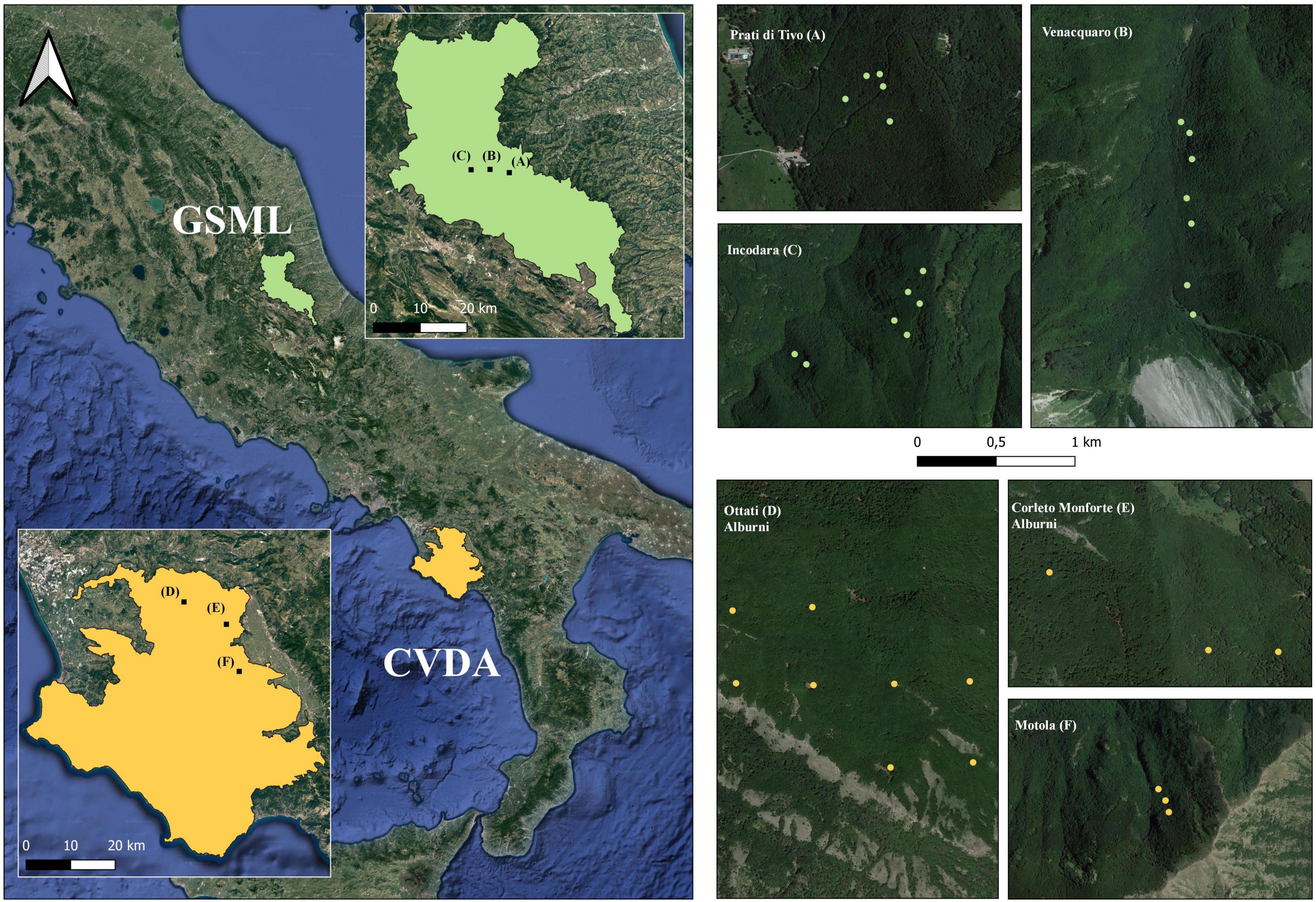
Figure 1. On the left, the National Parks where the study areas are located (GSML, Gran Sasso e Monti della Laga National Park; CVDA, Cilento, Vallo di Diano e Alburni National Park). In the magnification, black dots represent the study areas investigated in each park: in GSML, “Prati di Tivo”, “Venaquaro”, and “Incodara”; in CVDA, “Ottati”, “Corleto Monforte”, and “Motola”. On the right, the green and yellow dots represent the locations of the plots sampled in GSML and CVDA, respectively.

TABLE 1

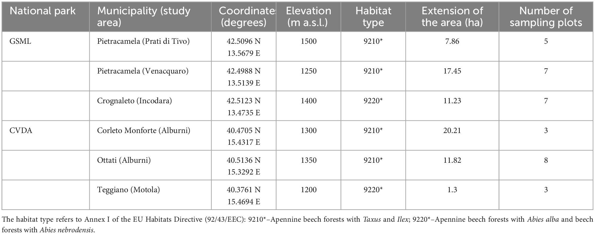
Table 1. Main characteristics of the study areas from Sabatini et al. (2016).

In each plot, the species diversity of different taxa was estimated using ad-hoc protocols for each taxon.

2.2.1. Saproxylic and non-saproxylic beetles and breeding birds

A sampling of beetle fauna was carried out using two methods: window flight traps for flying beetles and emergence traps for beetles moving on the surface of dead trunks/branches; both trap types were positioned at the center of each plot. Flight traps were checked approximately every 30 days for a total of four surveys from June to October 2016. Emergence traps were emptied only once at the end of the sampling period. All the monitoring systems were removed at the end of October. Systematics and nomenclature followed Bouchard et al. (2011), Audisio et al. (2015). All the taxa collected during the field surveys are alphabetically listed in Supplementary Table 1. In particular, species strictly considered as saproxylic (sensu Carpaneto et al., 2015) are reported together with their risk category at the Italian level see Audisio et al. (2015), Carpaneto et al. (2015).

For breeding birds, to coincide with the bird breeding season, surveys were carried out from May to June 2016, when the activities and the birdsong production intensify. Count points were positioned in each sampling plot, and the survey was carried out on three consecutive days in CVDA, and on 4 consecutive days in GSML. For discerning the bird species with a small home range, count points were at least 150 m apart. Each sample consisted of a 10-min count point, during which we recorded the richness and abundance of every species detected both visually and by hearing (Balestrieri et al., 2015). The species nomenclature follows Brichetti and Fracasso (2015) (see Supplementary Table 2).

2.2.2. Epiphytic lichens

Epiphytic lichens were sampled on the three beech trees (DBH ≥ 16 cm) nearest each plot’s center, using a portable 10 × 50 cm frame composed of five 10 × 10 cm quadrats. The frame was placed on the tree trunk facing the four cardinal directions, with the bottom part at a height of 1 m from the ground. All the species inside the frames were considered; thus, at the plot level, lichen richness equaled the total number of species occurring across the three sampled trees. While species frequency was computed as the proportion of 60 quadrats (10 × 10 cm) in which the species occurred. The protocol follows the European guidelines for lichen monitoring (Asta et al., 2002), while nomenclature and general information on species’ biological traits and ecology were retrieved from Nimis (2021) (see Supplementary Table 3).

2.3. Sentinel-2 data

Sentinel-2 (S2) is a European Space Agency (ESA) wide-swath, fine-resolution, multispectral imaging satellite mission. The revisit frequency is 5 days at the global scale, while 2 to 3 days at mid-latitude. The S2 Multispectral Instrument (MSI) samples 14 spectral bands (B): visible (B2, B3, B4) and nir (B8) at 10 m, red-Edge (B5, B6, B7, B8a), and swir (B11, B22) at 20 m, and four atmospheric bands (B1, B9, B10, QA60) at 60 m spatial resolution. QA60 is a bitmask band with dense and cirrus cloud information (Cloud mask). The complete S2 imagery archive can be found in Google Earth Engine GEE (Gorelick et al., 2017), with a detailed description of data, available bands, image properties, and terms of use.¹

We selected all S2 imagery acquired over the study area between 2017-09-01 and 2021-08-31, with a cloud cover smaller than 70%. A so long time series – combined with the 5-day revisitation time of the S2 mission–ensures having a large number of imagery, that is needed to properly calculate harmonic metrics (Shumway and Stoffer, 2017). To mask out clouds and cirrus from imageries, we used the S2 cloud probability dataset, which was created using the gradient boost base algorithm. More information on the Sentinel-2 cloud detector algorithm can be found on GitHub.² We resampled all bands to the finest spatial resolution of 10 m. Finally, the pixel values were extracted at the center location of each plot using a buffer of 13 m radius. The final values reported for each plot were the mean value of all pixels inside the buffer weighted by the coverage fraction of each pixel.

3. Methods

3.1. Sentinel-2 harmonic metrics and seasonal composites

Using the mentioned S2 images, we calculated a set of 91 harmonic metrics. First, we increased the number of variables for each S2 image by augmenting available bands [blue, green, red, red-Edge (redE)1, redE2, redE3, nir, redE4, swir1, swir2] by calculating the Normalized Difference Vegetation Index NDVI, the Normalized Burnt Ratio NBR, the Enhanced Vegetation Index EVI, and the Tasseled Cap Brightness TCB, Wetness TCW, Greeness TCG and Angle TCA indices. While several additional indices can be calculated using S2 data,³ those selected in this study represent a standard in remote sensing analysis and are those most commonly exploited (Hermosilla et al., 2015; Jönsson et al., 2018). In particular, the NDVI has become a standard since its introduction by Rouse et al. (1973) and has been applied to a wide range of practical remote sensing applications (Tucker et al., 1985; Wang et al., 2005; Zarco-Tejada et al., 2005; Beck et al., 2006). The NDVI index (Eq. 1) has been among the most popular indices used to delineate vegetation and vegetative stress quickly. Hence, it shows dense vegetation with high positive values, soil with low positive values, and water with negative values (Huang et al., 2021). The EVI index is instead known as it does not saturate as rapidly as NDVI in dense vegetation and it has been shown to be highly correlated with photosynthesis, plant transpiration, and vegetation biomass in a number of studies (Sims et al., 2006; Jiang et al., 2008). Finally, the NBR is the most commonly used index for forest disturbance monitoring, including forest fires, harvestings, and drought (Kennedy et al., 2010; Hansen et al., 2013; Francini et al., 2021), and it was exploited in this study to detect eventual stress status over our study areas.

Exploiting those indices, harmonic metrics were calculated (Figure 2). Four harmonic function coefficients were then calculated to identify the pixel harmonic trend (Shumway and Stoffer, 2017). Each pixel harmonic trend function was further used to calculate the amplitude, the phase, and the root mean square error (RMSE). As a result, we obtained a set of 13 (the bands plus the indices) * 7 (the harmonic function coefficients plus the amplitude, phase, and RMSE) = 91 harmonic metrics.

FIGURE 2

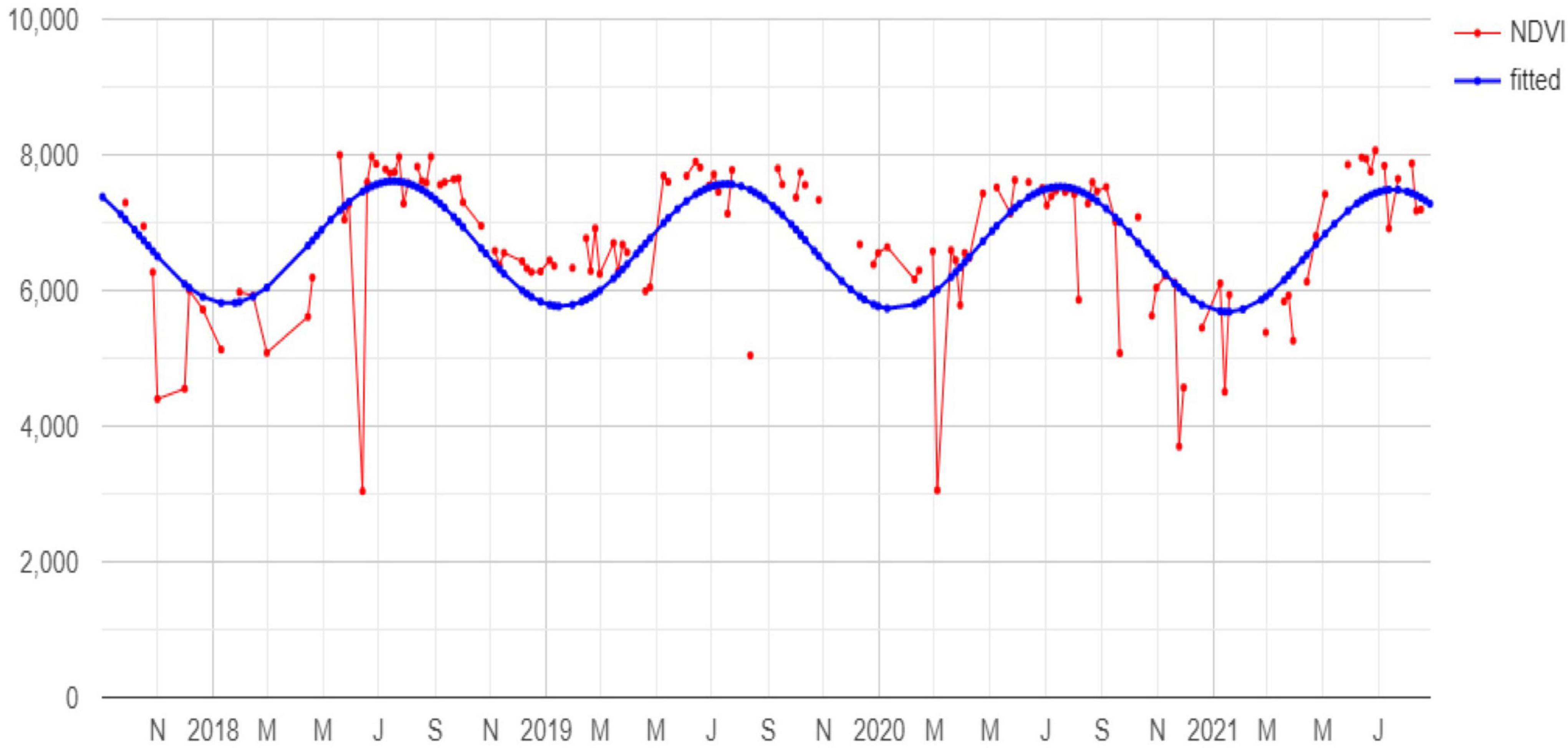
Figure 2. Example of NDVI pixel time series (red) and the corresponding fitted harmonic function (blue).

3.2. Diversity indices

Species diversity was calculated separately for each taxon and among taxa, using univariate diversity indices, incorporating the number of species and their relative abundance. We computed two different indices:

(i) Shannon’s entropy index (Eq. 1), which considers species frequency in the plot and can be interpreted as the effective number of species in the community.

$H^{\prime }=-{\sum }_{i=1}^S{p}_i\log p_i(1)$

Where S is the number of species in the assemblage, and p_i is the relative abundance of ith species.

(ii) Simpson’s diversity index (Eq. 2), which places more weight on the frequencies of abundant species, discounting rare species. It can be interpreted as the effective number of dominant species in the assemblage.

$D={\sum }_{i=1}^S{p}_i^2(2)$

We also compared the species diversity across assemblages, using rarefaction and extrapolation curves, provided by Hsieh et al. (2016) for the two members of the Hill number.

Finally, we compared the two study areas regarding species diversity. Firstly, we analyzed the variance and distribution of variables with the F-test and Shapiro-Wilk test, which are useful to check whether to use a parametric or non-parametric test. Then, the variables normally distributed that satisfied the conditions of homogeneity of variance were compared with the independent T-test. At the same time, the remaining variables were tested with the Wilcoxon-Mann-Whitney test.

3.3. Multi-taxon communities and relationships between harmonic metrics

For each taxon and the whole multi-taxon community, we verified possible relationships between harmonic metrics and the species diversity in terms of Shannon’s and Simpson’s biodiversity indices. Pearson’s product-moment correlation (r) matrix between each harmonic metric, species diversity, and structural variables was calculated separately for each study site to test the generalizability and consistency of the results when different remotely sensed imagery acquired in different conditions are available.

3.4. Random forests

Correlations are often not sufficient to estimate the predictive ability of the proposed metrics, as well as potential biases in a modeling task. To assess the potential of these metrics in predicting species diversity in terms of Shannon’s and Simpson’s biodiversity indices and to simplify the computation time for a regular application of this method, we fitted a random forests (RF) model between each diversity index and the best 10 harmonic metrics (in terms of absolute correlation, that is, the magnitude of the correlation) for each taxon combining data from the two study areas. Differently from the correlations, the limited number of samples per study area (19 in GSML and 14 in CDVA) was not sufficient to properly train and validate the model robustly.

Random forests (RF) is a popular machine-learning model that generates a set of decision trees ensembled to produce predictions. Each decision tree in the “forest” is built using different training subsets generated from the initial training dataset by a bootstrap procedure and a randomly chosen subset of predictors at each splitting node to minimize the correlation among trees. RF can reduce the output variance and the overfitting problem with respect to other machine-learning approaches, improving model stability and accuracy (Breiman, 2001).

Random forests (RF) permits the in-built estimation of variables’ importance from the out-of-bag (OOB) samples, that is, the samples randomly left out in the bootstrap procedure, by calculating the percent increase in the mean squared error (%incMSE) when the OOB data for each variable are permutated. The more the MSE increases from the permutation of a given variable, the more important the variable is in the model.

Models’ performance was evaluated using the leave-one-out (LOO) cross-validation technique (also known as Jack-knife), where each observation in the training set is left out in sequence, and its value is predicted using the remaining observations (McRoberts et al., 2015). For each model, we calculated the LOO root mean square error (RMSE) relative to the mean values of the observation:

$RMSE=\sqrt{\frac{{\sum }_{i=1}^n{(y_i-\widehat{y_i})}^2}{n}}$

Where n is the number of filed plots, y_i is the observed value and $\widehat{y_i}$ is the predicted one.

Each model was fitted using all field plots available (i.e., 33) to ensure the statistical robustness of the results.

The RF analysis was conducted using the randomForest R package within the R software version 4.2.0 (Liaw and Wiener, 2002).⁴ The hyperparameters were left to their default values, that is, 500 number of trees and a mtry values of p/3 where p is the number of predictors.

4. Results

4.1. Saproxylic and non-saproxylic beetles, and breeding birds

In GSML and CVDA, a total of 2,076 and 1,353 beetle specimens were collected, respectively, as well as 35 and 36 families.

In GSML, Elateridae was the most common family (32% of the total specimens collected): one species, Nothodes parvulus, represented over 22% of the family sampled, with 472 sampled specimens. Elateridae were followed by Cerambycidae (17.6%), Melyridae (11.6%), and Curculionidae (9.4%). The remaining families represent less than 29% of the total sampled families.

Whereas in CVDA, the most abundant species were Dalopius marginatus (Elateridae), with 142 specimens, Dasytes (Mesodasytes) plumbeus (Melyridae) were 125, while Phyllobius (Dieletus) argentatus (Curculionidae), with 83 specimens, corresponded to the 25.8% of the total sampled species. Similarly to GSML, Elateridae represented 0.7% of the total specimens, followed by Curculionidae (14.5%), Melyridae (10%), Tenebrionidae (7.4%), Staphylinidae (6.7%), and Cerambycidae (3%). The remaining families represented 23% of the total [see Supplementary Table 1, data reported by Campanaro and Parisi (2021)].

In addition, among the 164 collected species in GSML, 76 (46.3%) were saproxylic, and among them, 25 species (32.8%) are included in the Italian Red List for saproxylic beetles (Carpaneto et al., 2015). Of these, 17 species belong to the Near Threatened (NT), two to the Vulnerable (VU), and two to the Critically Endangered (CR) categories. One refers to each of the Endangered (EN), and four species are attributable to the DD (Data Deficient) category (Supplementary Table 1).

According to the trophic categories in GSML, saproxylophagous represented 27.6% of the total sampled families, followed by Xylophagous (18%), Mycophagous (18.4%), Predators (17%), Mycetobiontic (5%), while for the trophic categories: Sap-feeder, HW (associated with small water pools inside hollow trees), NI (inhabiting birds “and small mammals” nests in hollow trees) and Unknown only one specimen was collected.

Instead, in CVDA, on a total of 183 collected species, 76 (41.5%) were saproxylic. Among them, 25 species (32.8%) are listed in the Italian Red List for saproxylic beetles (Carpaneto et al., 2015): 17 species belong to the NT, while three to the VU and two to CR categories. One refers to each EN, and two species are attributable to the DD category (Supplementary Table 1). Only one specimen was collected from Saprophytophagous and HW.

Regarding the breeding birds, twenty-seven bird species (21 in GSML and 20 in CVDA) and 17 families were recorded. Furthermore, two species are included in the Red List Categories. In particular, Emberiza citrinella (Emberizidae) for the VU category was recorded in GSML, and the Fringillidae Pyrrhula pyrrhula for the NT category was observed in both national parks. Finally, two species are exclusive for GSML and five for CVDA (see Supplementary Table 2).

4.2. Epiphytic lichens

For lichens, 59 species were totally recorded for both the study areas, 43 in GSML and 51 in CVDA. Specifically, seven species are exclusive in GSML and 15 in CVDA. Regarding the families, 15 and 17 families were respectively sampled. The Parmeliaceae family was the most common in both areas, followed by the Lecanoraceae. The most frequent species were Lecidella elaeochroma, followed by Lecanora intumescens and L. albella (Lecanoraceae) in GSML, and Phlyctis argena (Phlyctidaceae) followed by L. ealeochroma and Parmelia saxatilis (Parmeliaceae) in CVDA. Among the species registered, a few are of conservation interest. Anaptychia crinalis and Lepra slesvicensis are included in the Italian Red List of epiphytic lichens as VU and DD, respectively (Nascimbene et al., 2013); in addition, Bryoria nadvornikiana is considered as an indicator of forest oldgrowthness (Holien, 1989). Lobaria pulmonaria was also observed: it is an “umbrella species,” since its frequency is strongly related to the number and frequency of other species in the ecological community of its habitat (Nascimbene et al., 2010) (see Supplementary Table 3).

4.3. Diversity indices

The values of the Shannon’s and Simpson’s diversity indices in the two study areas are shown in Supplementary material (Supplementary Figure 1), for the whole communities and grouped by taxa.

The diversity indices analyzed were consistently higher for the multi-taxon community than for the single taxon; moreover, they were generally higher in CVDA than in GSML, except for the bird community, where all the indices were higher in GSML. Regarding Shannon’s entropy index, the number of equally common species was generally higher in CVDA, except for the bird community. The Simpson’s diversity index showed a similar pattern for each taxon but with a narrower distribution around the highest value in CVDA.

Figure 3 shows the rarefaction and extrapolated curves for each taxon in relation to the two diversity indices. The Shannon’s and Simpson’s biodiversity indices showed similar patterns for each taxon, indicating that the number of equally common species and the dominant ones was higher in CVDA than in GSML, for the beetle and lichen communities. In contrast, the bird community reached the same diversity level in both study areas. From the extrapolated curve, it can be stated that the sampling effort was adequate to describe the species diversity in each taxon and for both the sampled areas.

FIGURE 3

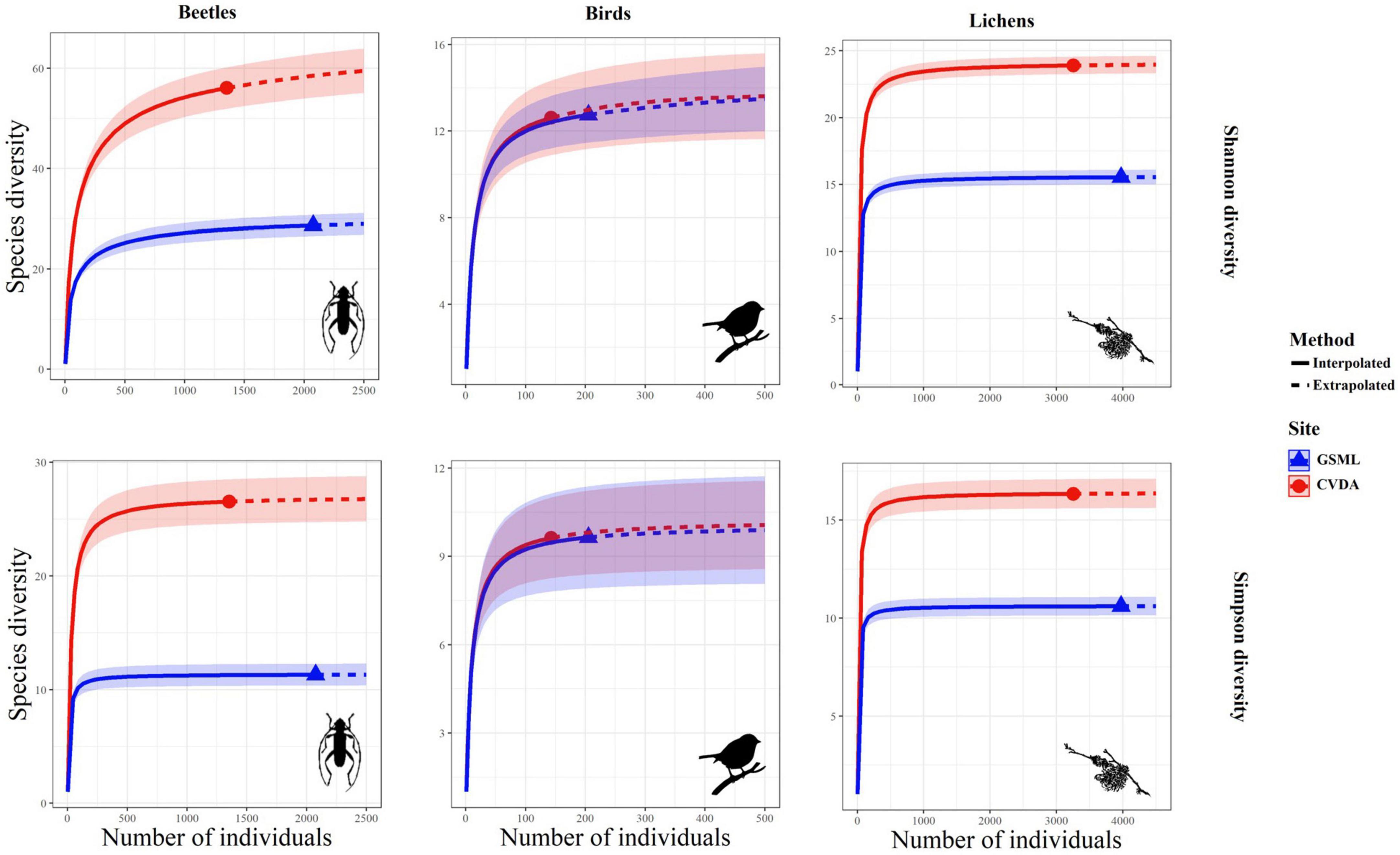
Figure 3. Rarefaction curves with 95% confidence intervals (shaded areas) for two biodiversity indices (Shannon and Simpson) for the three taxa considered.

Regarding the two study areas, the analysis of the T-test and the Wilcoxon-Mann-Whitney test revealed that the diversity indices were always significantly different for the multi-taxon and lichen communities (Table 2). The beetle community differed in terms of Shannon’s biodiversity index, while minor discrepancies were observed for the Simpson’s diversity index, indicating similar dominant species diversity between areas. In contrast, no significant differences were found between areas regarding all the diversity indices analyzed in the bird community.

TABLE 2

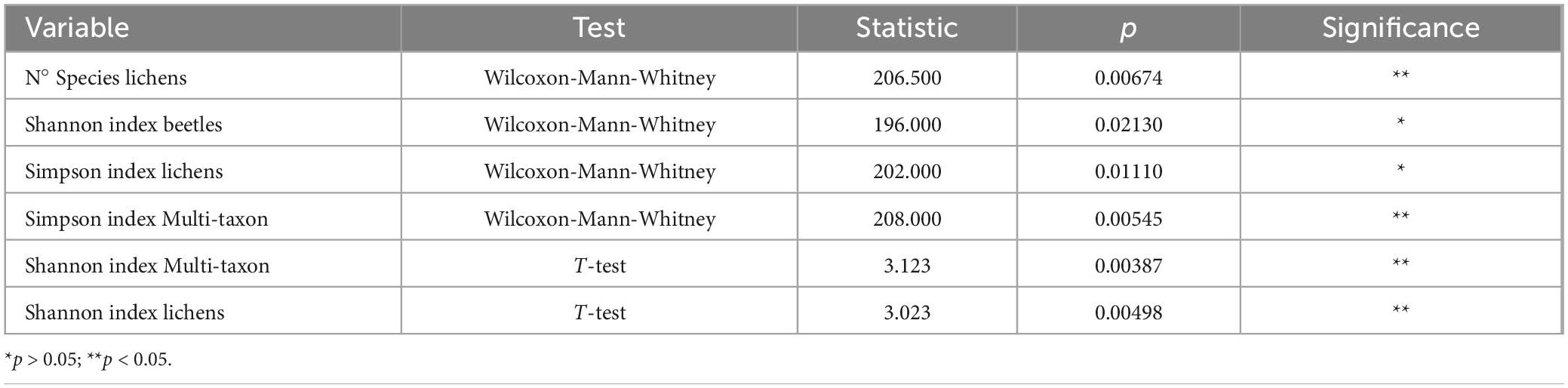
Table 2. Differences between the study areas in terms of species diversity.

Based on the relationships between S2 harmonic’s temporal metrics (TMs) and diversity indices among the taxa communities, the strongest correlations were reached in CVDA. The multi-taxon and beetle communities reached the highest correlation values, with a median absolute correlation of 0.52 and 0.38, respectively, followed by the lichen and bird communities with 0.28 and 0.15, respectively. Shannon’s biodiversity index reached similar correlation values, regardless of the community, while Simpson’s diversity index generally obtained lower correlations. The bands that obtained the strongest correlation were swir1 and 2, followed by the redE bands and the photosynthetic indices (firstly, the tasseled cap indices, followed by NDVI and NBR), all with an absolute correlation coefficient (hereinafter referred to | r|) > 0.3. Finally, the best harmonic metrics were the cosine, phase, and amplitude (| r| > 0.35), followed by constant and sine, and the RMSE reached the lowest absolute median correlation (| r| = 0.18). Figure 4 shows Pearson’s product-moment correlation (r) between the diversity of each taxon, in terms of Shannon’s and Simpson’s biodiversity indices, and the seven harmonic TMs calculated for each S2 band and index in the CVDA site.

FIGURE 4

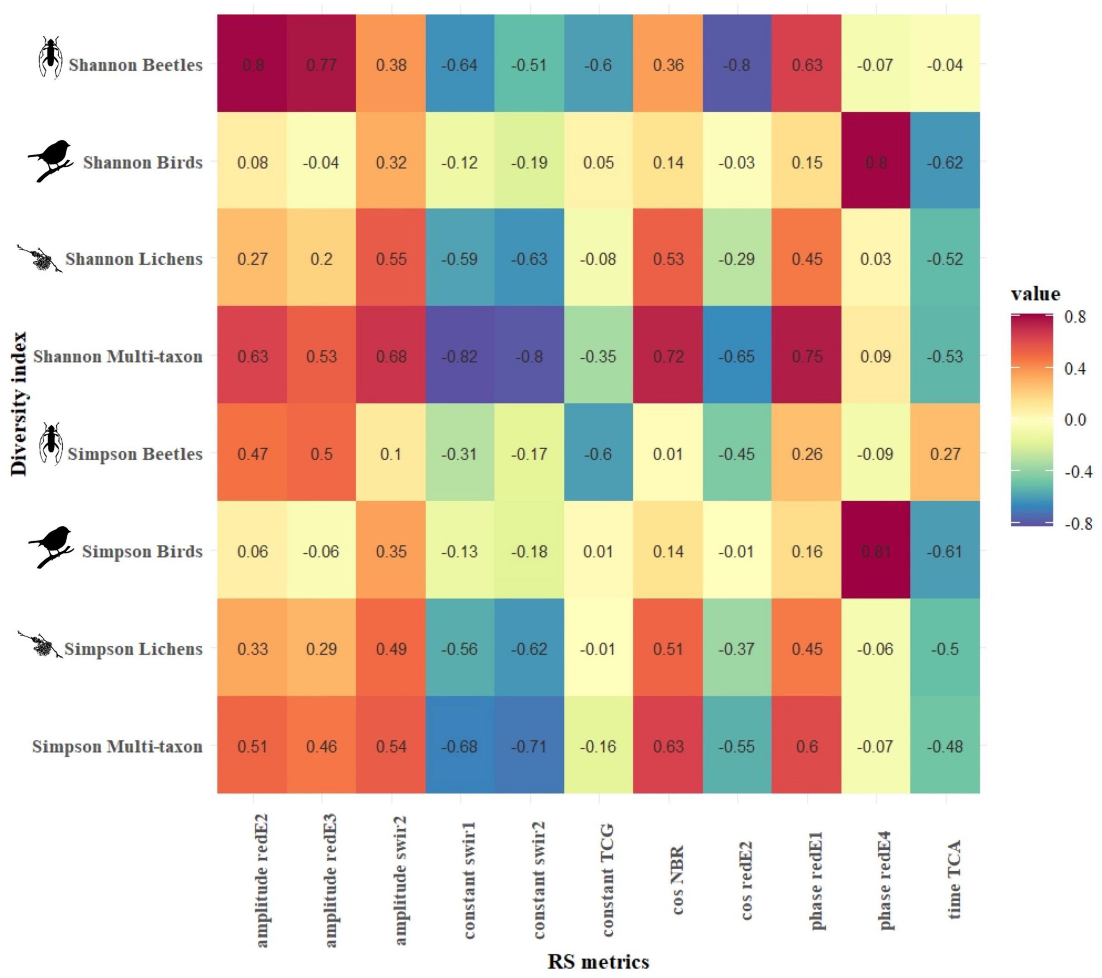
Figure 4. CVDA: Pearson’s product-moment correlation (r) between biodiversity indices of each taxon (y-axis) and the best Sentinel-2-derived temporal metrics (x-axis). The color in each cell represents the correlation value between the corresponding variables in the two axes.

Figures 4, 5 present the highest correlation achieved by each combination of harmonic metrics and diversity index for CVDA and GSLM, respectively. In CVDA (Figure 4), correlations were generally lower. However, absolute maximums were similar between the two study areas (maximum positive correlation of 0.8 between Shannon’s diversity index for the beetle community and the amplitude of the red-Edge 2, and maximum negative correlation of −0.81 between the Simpson’s diversity index for the lichen community and the sine of TCG index). In GSML, the highest median absolute correlation was obtained by the lichen community (| r| = 0.34), followed by the beetle and multi-taxon communities (| r| = 0.26 and | r| = 0.19, respectively), with the bird community reaching the lowest value (| r| = 0.10). Results did not match between areas, also in terms of diversity indices. In GSML, all diversity indices reached similar correlation values (| r| between 0.19 and 0.21). The correlation achieved by photosynthetic indices exceeded that of all the other S2 bands, with EVI, NDVI, and NBR overcoming tasseled cap indices, swir, and red-Edge bands. Finally, the harmonic metric, which obtained the highest median absolute correlation, was the constant (| r| > 0.23), followed by amplitude, cosine, sine, and RMSE (| r| > 0.21). At the same time, time and phase achieved the lowest absolute median correlation (| r| < 0.20) (Figure 5).

FIGURE 5

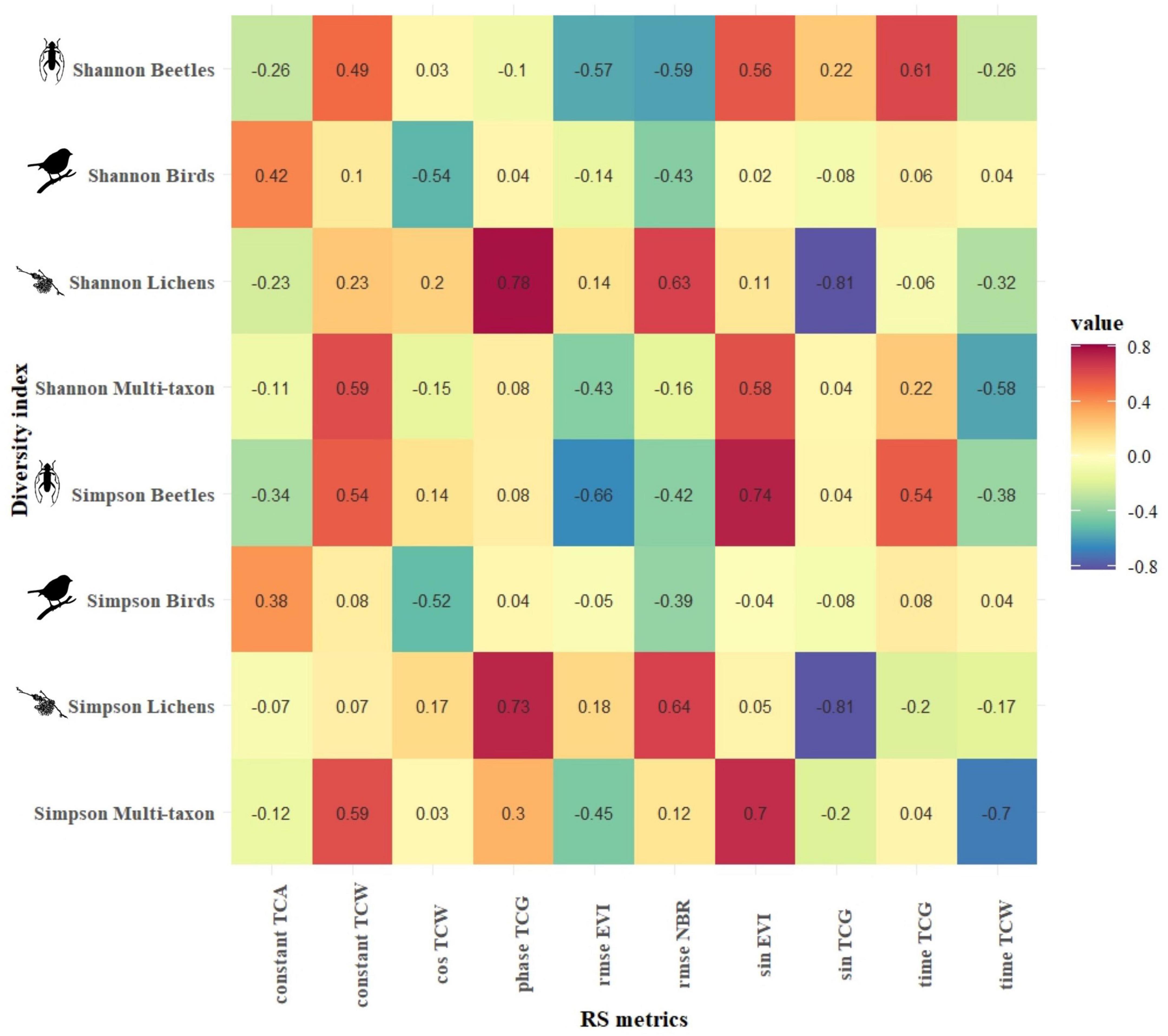
Figure 5. GSML: Pearson’s product-moment correlation (r) between biodiversity indices of each taxon (y-axis) and the best Sentinel-2-derived temporal metrics (x-axis). The color in each cell represents the correlation value between the corresponding variables in the two axes.

4.5. Random forests

According to the importance of the variables, the phase and RMSE of red-Edge bands were the most important for describing the diversity of birds and lichens communities, while beetles and multi-taxon diversity were better predicted from RMSE and time of tasseled cap and EVI indices (Figure 6). The % of variance explained was internally calculated by RF from the OOB observations and ranged between 17.0 and 35.8 and between 16.7 and 22.2 for Shannon’s and Simpson’s diversity indices, respectively. The maximum was reached by the multi-taxon and bird communities for the Shannon and the Simpson index, respectively (Table 3; see Section “3.4. Random forests”). The RMSE% were generally lower for Simpson’s diversity index, spanning from 2.53 to 9.99 (for the multi-taxon and beetles community, respectively), while for Shannon’s diversity index ranging between 8.1 and 16.8 (for the multi-taxon and lichens community, respectively) (Figure 7).

FIGURE 6

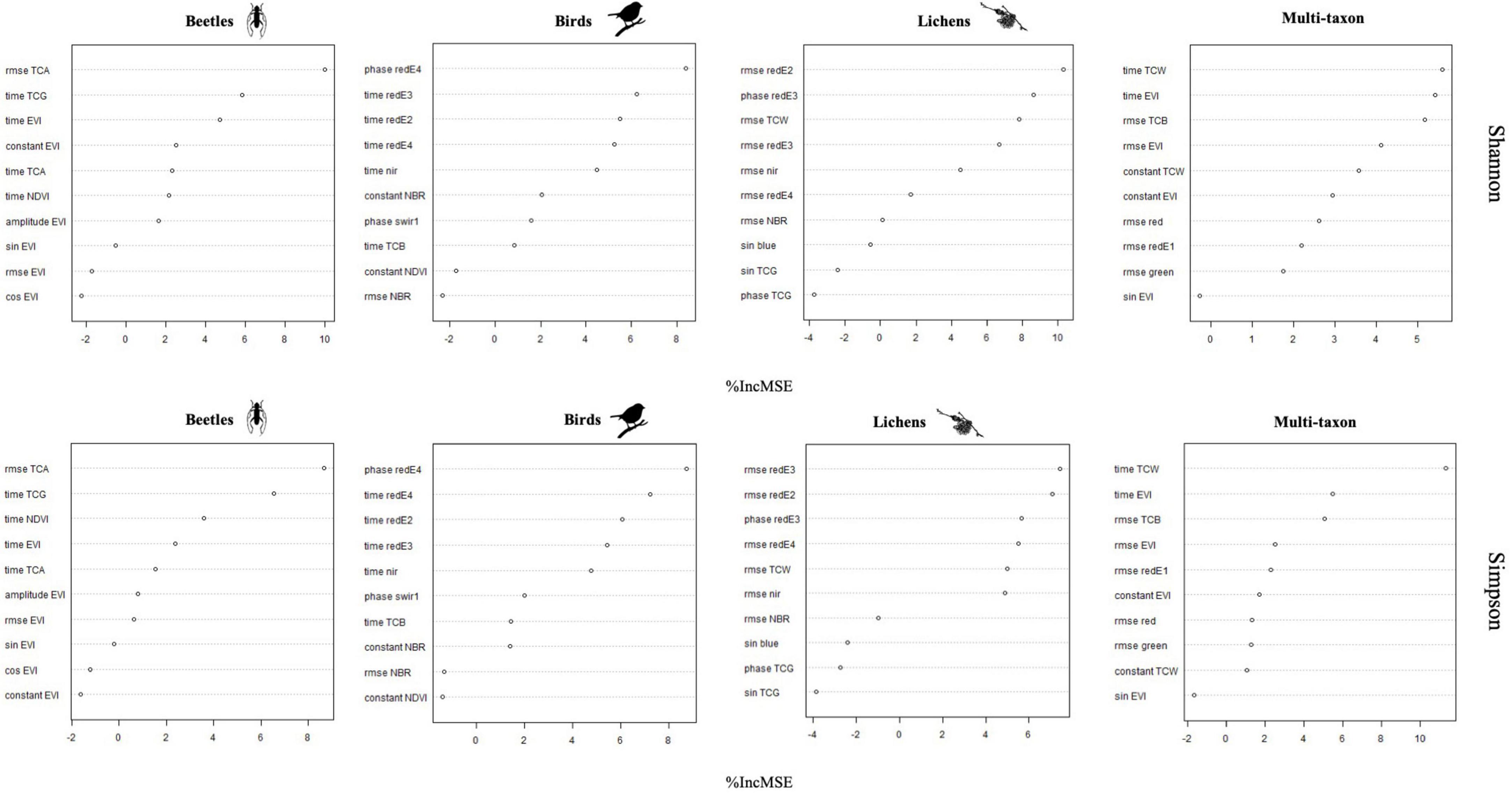
Figure 6. Variables importance for each of the eight random forests (RF) models.

TABLE 3

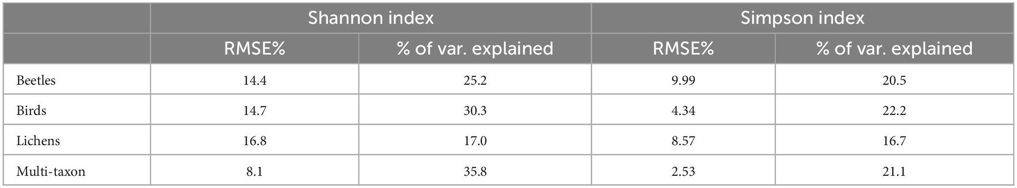
Table 3. Leave-one-out (LOO) root mean square error (RMSE)% and % of variance explained obtained by random forests (RF) models fitted with the best 10 harmonic metrics for each diversity index.

FIGURE 7

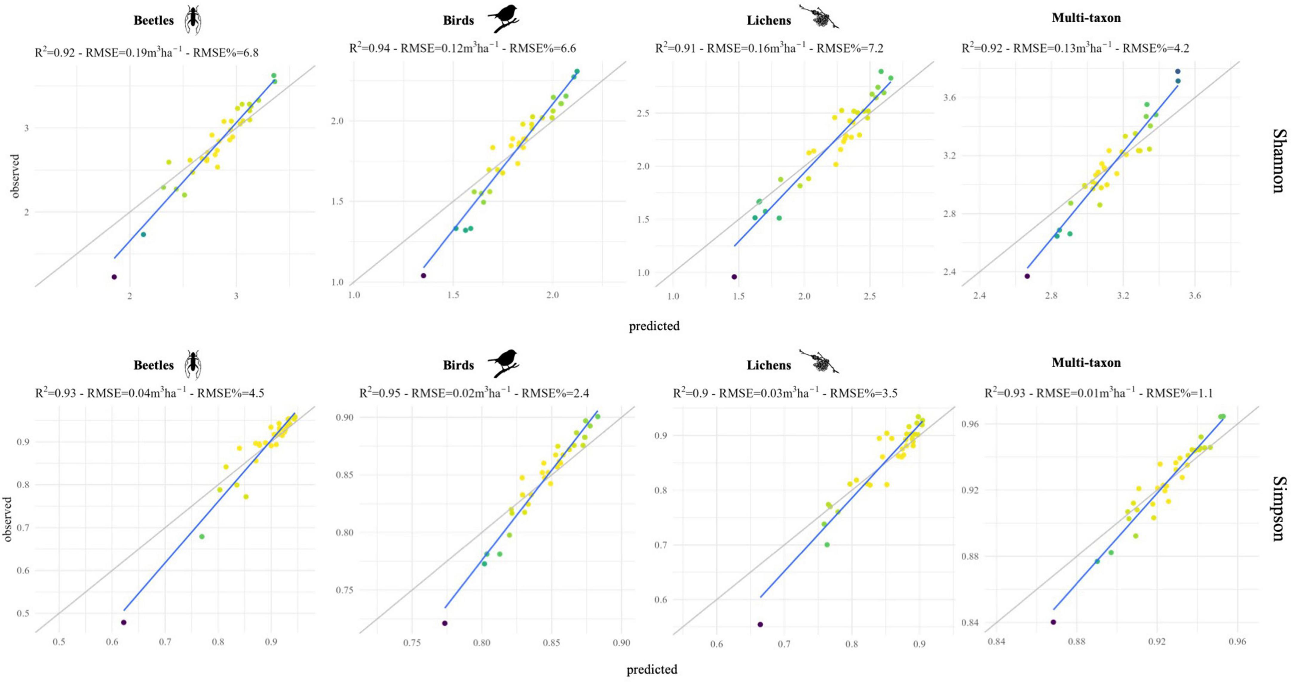
Figure 7. Scatterplot of predicted vs. observed values for each diversity index and taxon, obtained with random forests (RF) models. Colors represent the point density.

5. Discussion

5.1. Diversity indices

The Shannon’s and Simpson’s diversity indices showed higher values for beetles and lichens in CVDA, while in GSML, the diversity indices had comparatively higher values for birds. No significant differences were found between the two areas regarding diversity as a whole (multi-taxon). The biodiversity indices showed similar and homogeneous diversity and species richness values in GSML and CVDA. This was confirmed by Shannon’s diversity index, which indicates a lack of similarity in the distribution of dominant species. On the other hand, the diversity indices suggested differences in species composition between these two protected areas (GSML and CVDA).

The beetle community included abundant and threatened species (see Supplementary Table 1). Elateridae (beetles) dominated both areas, with two different species (Nothodes parvulus and Dalopius marginatus, respectively, in GSML and CVDA) being the most abundant (22% of the total species). The abundance of the two taxa probably influenced the diversity analysis as total individuals for this group.

Few differences were found between the areas when considering birds (21 in GSML and 20 in CVDA) and lichens (43 in GSML and 51 in CVDA). Overall, CVDA showed a more uniform number of individuals per species than GSML, as confirmed by the biodiversity indices (i.e., number of taxa). This might depend on the presence of large trees, hosting a great abundance of lichens and providing numerous microhabitats for the fauna, ensuring essential habitat and resource availability over time and space often missing from small trees see Sabatini et al. (2016), Parisi et al. (2021). Thus, growing large trees might allow more stable environmental conditions in terms of ecological continuity and promote the stability of the multi-taxon communities (Basile et al., 2020), though their vulnerability to disturbances (e.g., windthrow) needs to be considered. As reported by Feest et al. (2010), a site may have a biodiversity quality that is dominated by the high biomass of a few species (low species richness), in contrast to another site where the opposite prevails. Finally, the two areas were highly different in terms of mean of growing stock volume (GSV) (688 m³ ha^–1 for GSML and 331 m³ ha^–1 for CVDA) see Parisi et al. (2021).

5.2. Remote sensing metrics

From the analysis of RS metrics, the bands that obtained the strongest correlation between variables in CVDA were swir1 and 2, and the red-Edge bands, followed by the photosynthetic indices, while the best harmonic metrics were the cosine, phase, and amplitude (Figure 4). In contrast, in GSML, the strongest correlation between variables was achieved by photosynthetic indices, followed by swir, and red-Edge bands, while the best harmonic metric, were the constant, amplitude, cosine, sine, and RMSE (Figure 5).

Within RS metrics, NDVI, being related to forest structure, was associated with the abundance of the different taxonomic groups. Indeed, since some families of saproxylic and non-saproxylic beetles need direct solar radiation and low tree cover (low NDVI) to perform their biological functions, an inverse correlation between RS metrics and species abundance could be expected. The same considerations could be made for epiphytic lichens, whose richness should be higher in forests with higher light penetration. On the other hand, S2 indices related to the photosynthetic activity (EVI, NDVI, and NBR) could directly or indirectly be linked to the diversity and abundance of saproxylic species, depending on the biological activity of adults and pollination (Thorn et al., 2020).

The relationship between satellite variables and multi-taxon biodiversity has been rarely explored, especially considering a comprehensive spatial extension (Müller and Brandl, 2009; Bae et al., 2019; Knuff et al., 2020; Parisi et al., 2022a). Indeed, when the spatial scale is large, a greater environmental variability is sampled and, therefore, the models of the different taxa are more likely to work better, also because of the common biogeographic and evolutionary history shared by taxa (Gioria et al., 2011; Rooney and Azeria, 2015). Furthermore, larger species pools provide greater biological resolution to detect changes in environmental conditions (Rooney and Azeria, 2015; Sabatini et al., 2016).

In this context, our analysis considered a data set with a limited number of sampling plots (33) and was focused on relatively well-preserved and low-intensively managed Mediterranean mountain forests dominated by beech; moreover, we only explored the relationship between taxa and S2 temporal series. It is possible to exclude that sampling comprised a broad environmental gradient, resulting in stronger correlations between the S2 temporal series and forest variables. When populations characterized by different conservation statuses, management regimes, or disturbance legacy are considered, stronger relationships between taxa and time series are more probable to occur than when considering relatively similar populations, as in the present case see Parisi et al. (2022a).

Likewise, a larger number of sampling areas may also improve results. Satellite data providing canopy-level information cannot fully describe the biodiversity of an ecosystem and cannot completely replace field surveys. On the other hand, based on highly repeatable and freely available RS data, they can be used at different spatial and temporal scales supporting the fieldwork limitations (Turner et al., 2003; Cerrejón et al., 2020). In the context of conservation priorities, the S2-derived harmonic metrics provided detailed and free information that might comprehensively complement ground data (Parisi et al., 2022b). While 10 m resolution may limit the capability to monitor small-scale relevant components of forest biodiversity, high-resolution images present some limitations. First, they are usually acquired with a lower revisitation time, compromising the capability to perform time series analysis and effective monitoring. Second, they are not open access and, therefore, unsuitable for large-scale biodiversity monitoring or nature-based forest management.

In this study, S2 variables were found to be a crucial component for the occurrence and distribution of the taxa examined. Indeed, our analyses show that some S2 variables (amplitude, cosine, sine, and RMSE) were related to the abundance of beetles, birds, and lichens (see Supplementary Tables 1–3) in Mediterranean mountain forests and highlight the potential of RS in forest biodiversity monitoring. Consequently, we suggest that, given the valuable products of S2 images, also integrating structure-related RS data (i.e., lidar data), RS metrics and in situ monitoring activities should be combined for a highly cost-effective comprehensive assessment and regular monitoring of forest biodiversity. S2 data can, indeed, be an excellent source of complementary information to that acquired in the field, allowing to increase in the spatial and temporal scale of the analysis, while decreasing the effort required for field surveys. On the other hand, we stress that RS data may not replace data acquired in the field, which will be always needed for a complete and detailed monitoring of forest biodiversity.

Random forests (RF) model highlighted the importance of different harmonic metrics in the prediction of Shannon’s and Simpson’s diversity indices for the different taxa combining data from the two study areas. On the other hand, although the correlation analysis between remote sensing data and ground data was conducted individually for each study area to check the generalizability of the results, the number of samples per study area (19 in the GSML and 14 in the CDVA) was too small to adequately train and validate the random forest model. In particular, the results obtainable in the two study areas separately would depend on the limited training data available. The most relevant metrics for predicting diversity indices were: rmse TCA and time TCG for beetles, phase redE4 and time redE3 for birds, rmse redE2 and phase redE3 for lichens and time TCW and time EVI for multi-taxon (Figure 6). Indeed, harmonic metrics of redE, specifically sensitive to chlorophyll levels and their variations (Immitzer et al., 2019), and harmonic metrics of TC, indicators of forest dynamics and stand development over time (Lastovicka et al., 2020), are valuable for identifying ecosystem biotic diversity. Finally, based on the best 10 harmonic metrics identified for each taxon, the prediction models of Shannon’s and Simpson’s indices remarked the robust predictive ability of S2 data, with RMSE% always lower than 15% and down to 2.5%, which resulted in an agreement between predictions and observations with R² values consistently greater than 90% (Figure 7).

5.3. Ecological significance of the multi-taxon approach

The diversity of the species and taxa sampled in this work was reflected in their different ecological roles and features within the community. For instance, most of the sampled lichens are known to be common on beech (Ravera et al., 2006; Nimis, 2021) and the number of recorded species was comparable to similar studies done on the Apennines (Ravera et al., 2010; Frati et al., 2021). Significant differences between the two study areas were reflected in the frequency of crustose pioneer lichens (e.g., Arthoniaceae and Lecanoraceae) and common generalist species (e.g., Lecidella elaeochroma, Physcia adscendens), while most of the species of conservation interest were exclusive of the CVDA. Lobaria pulmonaria, found abundant and fertile in CVDA (Brunialti et al., 2015), has a long vegetative cycle (Scheidegger et al., 1998; Denison, 2003) and known to be an indicator species of forest areas characterized by long ecological continuity (Barkman, 1958; Gauslaa, 1985, 1994, 1995; Rose, 1988). The rarefaction curves show that a small number of lichens were sampled sufficiently to describe the diversity in the two areas (Figure 3).

The harmonic variables presented in this study allowed the diversity of saproxylic and non-saproxylic beetles to be analyzed. Sun exposure is an important ecological parameter for the development of saproxylic beetles since it determines the occurrence of different ecological niches and food substrates and, therefore, different trophic categories of insects (Parisi et al., 2019, 2022a). The areas with the greatest irradiance were characterized by a greater abundance of flowering and fruit plants, representing a key resource for many saproxylic beetles (Bouget et al., 2014; Sabatini et al., 2016). In fact, many beetles have a saproxylic behavior during their larval stage, while the adults are often found on flowering plants in the arboreal and herbaceous layers (Sabatini et al., 2016; Parisi et al., 2021). For instance, the Cerambycidae feed on decaying wood during the larval stage, while adults feed on the pollen of herbaceous species belonging to the Asteraceae and Apiaceae families.

Furthermore, Blasi et al. (2010) found a similarity between lichens and beetles in terms of light requirements in beech forests on the Apennines. Indeed, in forests with open overstory, where more light for photosynthesis is available, and the microclimate is relatively warmer, a greater density and diversity of undergrowth vegetation and epiphytic lichens are expected (Aragon et al., 2010; Sabatini et al., 2014; Klein et al., 2020). By contrast, birds usually require a denser understory, which provides protection from predators and suitable nesting sites (Klein et al., 2020).

6. Conclusion

We studied the capability of Sentinel-2 time series to monitor communities of beetles, birds, and lichens, both as individual taxonomic groupings and as multi-taxon in two beech forests in Mediterranean mountain areas. Results encourage researchers and managers to use RS data to identify, assess, and monitor potential biodiversity hotspots and, thus, to reduce the effort required for ground data acquisition. This is particularly relevant in impervious environments, such as those in mountain areas. S2 data may help improve the identification of areas for nature conservation and the management of threatened species by recognizing and quantifying habitat preferences and habitat-specific thresholds. Therefore, areas that should be prioritized as set-aside or core areas in forest stands and conservation plans could be identified by combining optical information with different RS data, such as ALS (Lindberg et al., 2015) or radar data (Bae et al., 2019). This may help achieve a multi-functional landscape, ensuring multiple uses of forests to balance biodiversity conservation and forest production at the landscape level (Muys et al., 2022).

We found seven species of beetles, two birds, and two lichens included in the IUCN Red List. The scarce and threatened taxa were collected only in some sites and with few individuals and could hardly be used as indicators (Supplementary Tables 1–3). In the next future, S2 time series analysis should evolve for creating statistically rigorous spatial estimation of indicators for monitoring forest structural complexity and multi-taxon forest communities (Mura et al., 2016), including threatened species, thus informing nature-based forest management. Such efforts will contribute to (i) achieving the objectives of the EU Biodiversity Strategy for 2030 (EU Biodiversity Strategy for 2030, 2020), (ii) implementing climate-smart forestry, (iii) planning strategies to conserve biodiversity in protected environments, and (iv) balancing conservation measures and silvicultural practices.

Finally, we suggest including other taxonomic groups, and the relative biomass proportions of each species (Feest et al., 2010), closely related to forest structural traits in future studies (e.g., small mammals, spiders, amphibians, fungi, and bryophytes), for a comprehensive ecosystem monitoring and, therefore, to track down biodiversity hotspots more effectively.

Data availability statement

The raw data supporting the conclusions of this article will be made available by the authors, without undue reservation.

Author contributions

FP, EV, SF, and GD’A: conceptualization, data curation, investigation, methodology, resources, roles/writing—original draft, and writing—review and editing. SR: resources, roles/writing—original draft, and writing—review and editing. ED: roles/writing—original draft and writing—review and editing. GC, MM, FL, DT, and RT: supervision and writing—review and editing. All authors contributed to manuscript revision, read, and approved the submitted version.

Acknowledgments

The authors thank the specialists of the various taxonomic groups: Paolo Audisio (Nitidulidae), Alessandro Bruno Biscaccianti (Alexiidae, Bethylidae, Cerylonidae, Dascillidae, Dermestidae, Erotylidae, Eupelmidae, Laemophloeidae, Lathridiidae, Lucanidae, Mycetophilidae, Salpingidae, Scirtidae, Sphindidae, Tenebrionidae, Trogossitidae), Enzo Colonnelli (Anthribidae, Attelabidae, Brentidae, Curculionidae), Gianluca Magnani (Buprestidae), Massimo Faccoli (Curculionidae Scolytinae), Fabrizio Fanti (Cantharidae, Lampyridae), Emanuele Piattella (Scarabaeidae), Giuseppe Platia (Elateridae), Roberto Poggi (Staphylinidae Pselaphinae), Pierpaolo Rapuzzi [Cerambycidae (pars)], Enrico Ruzzier (Mordellidae, Scraptiidae), and Adriano Zanetti [Staphylinidae (pars)]. We are grateful to Bruno Lasserre (Università degli Studi del Molise, Italy) for technical support.

Conflict of interest

The authors declare that the research was conducted in the absence of any commercial or financial relationships that could be construed as a potential conflict of interest.

Publisher’s note

All claims expressed in this article are solely those of the authors and do not necessarily represent those of their affiliated organizations, or those of the publisher, the editors and the reviewers. Any product that may be evaluated in this article, or claim that may be made by its manufacturer, is not guaranteed or endorsed by the publisher.

Supplementary material

The Supplementary Material for this article can be found online at: https://www.frontiersin.org/articles/10.3389/ffgc.2023.1020477/full#supplementary-material

Footnotes

1. ^ https://developers.google.com/earth-engine/datasets/catalog/sentinel-2
2. ^ https://github.com/sentinel-hub/sentinel2-cloud-detector
3. ^ https://www.indexdatabase.de/db/s-single.php?id=96
4. ^ https://www.r-project.org

References

Anderson, C. B. (2018). Biodiversity monitoring, earth observations and the ecology of scale. Ecol. Lett. 21, 1572–1585. doi: 10.1111/ele.13106

PubMed Abstract | CrossRef Full Text | Google Scholar

Aragon, G., Martínez, I., Izquierdo, P., Belinchón, R., and Escudero, A. (2010). Effects of forest management on epiphytic lichen diversity in mediterranean forests. Appl. Veg. Sci. 13, 183–194. doi: 10.1111/j.1654-109X.2009.01060.x

CrossRef Full Text | Google Scholar

Arekhi, M., Yılmaz, O. Y., Yılmaz, H., and Akyüz, Y. F. (2017). Can tree species diversity be assessed with Landsat data in a temperate forest? Environ. Monit. Assess. 189, 1–14. doi: 10.1007/s10661-017-6295-6

PubMed Abstract | CrossRef Full Text | Google Scholar

Asta, J., Erhardt, W., Ferretti, M., Fornasier, F., Kirschbaum, U., Nimis, P. L., et al. (2002). “Mapping lichen diversity as an indicator of environmental quality,” in Monitoring with lichens – monitoring lichens. Kluwer, NATO science series, Vol. 7, eds P. L. Nimis, C. Scheidegger, and P. Wolseley (Dordrecht: Springer), 273–279.

Google Scholar

Audisio, P., Alonso-Zarazaga, M., Slipinski, A., Nilsson, A., Jelínek, J., Vigna Taglianti, A., et al. (2015). Fauna Europaea: Coleoptera 2 (excl. series Elateriformia, Scarabaeiformia, Staphyliniformia and superfamily Curculionoidea). Biodivers. Data J. 3:4750. doi: 10.3897/BDJ.3.e4750

PubMed Abstract | CrossRef Full Text | Google Scholar

Bae, S., Levick, S. R., Heidrich, L., Magdon, P., Leutner, B. F., Wollauer, S., et al. (2019). Radar vision in the mapping of forest biodiversity from space. Nat. Commun. 10:4757. doi: 10.1038/s41467-019-12737-x

PubMed Abstract | CrossRef Full Text | Google Scholar

Balestrieri, R., Basile, M., Posillico, M., Altea, T., De Cinti, B., and Matteucci, G. (2015). A guild-based approach to assessing the influence of beech forest structure on bird communities. For. Ecol. Manage. 356, 216–223. doi: 10.1016/j.foreco.2015.07.011

CrossRef Full Text | Google Scholar

Barkman, J. J. (1958). Phytosociology and ecology of cryptogamic epiphytes. Assen: Van Gorcum, Comp. NV.

Google Scholar

Basile, M., Asbeck, T., Jonker, M., Knuff, A. K., Bauhus, J., Braunisch, V., et al. (2020). What do tree-related microhabitats tell us about the abundance of forest-dwelling bats, birds, and insects? J. Environ. Manage. 264:110401. doi: 10.1016/j.jenvman.2020.110401

PubMed Abstract | CrossRef Full Text | Google Scholar

Beck, P. S., Atzberger, C., Høgda, K. A., Johansen, B., and Skidmore, A. K. (2006). Improved monitoring of vegetation dynamics at very high latitudes: A new method using MODIS NDVI. Remote Sens. Environ. 100, 321–334. doi: 10.1016/j.rse.2005.10.021

CrossRef Full Text | Google Scholar

Blasi, C., Marchetti, M., Chiavetta, U., Aleffi, M., Audisio, P., Azzella, M. M., et al. (2010). Multi-taxon and forest structure sampling for identification of indicators and monitoring of old-growth forest. Plant Biosyst. 144, 160–170.

Google Scholar

Bombi, P., Gnetti, V., D’Andrea, E., De Cinti, B., Taglianti, A. V., Bologna, M. A., et al. (2019). Identifying priority sites for insect conservation in forest ecosystems at high resolution: The potential of LiDAR data. J. Insect Conserv. 23, 689–698. doi: 10.1007/s10841-019-00162-w

CrossRef Full Text | Google Scholar

Bouchard, P., Bousquet, Y., Davies, A. E., Alonso-Zarazaga, M. A., Lawrence, J. F., Lyal, C. H. C., et al. (2011). Family-group names in Coleoptera (Insecta). ZooKeys 88, 1–972. doi: 10.3897/zookeys.88.807

PubMed Abstract | CrossRef Full Text | Google Scholar

Bouget, C., Larrieu, L., and Brin, A. (2014). Key features for saproxylic beetle diversity derived from rapid habitat assessment in temperate forests. Ecol. Indic. 36, 656–664. doi: 10.1016/j.ecolind.2013.09.031

CrossRef Full Text | Google Scholar

Breiman, L. (2001). Random forests. Mach. Learn. 45, 5–32. doi: 10.1023/A:1010933404324

CrossRef Full Text | Google Scholar

Brichetti, P., and Fracasso, G. (2015). Check-list degli uccelli italiani aggiornata al 2014. Riv. Ital. Orn. 85, 31–50.

Google Scholar

Brunialti, G., Frati, L., and Ravera, S. (2015). “Ecology and conservation of the sensitive lichen Lobaria pulmonaria in Mediterranean old-growth forests,” in Old-growth forests and coniferous forests. Ecology, habitat and conservation, ed. P. Weber (Hauppauge, NY: Nova Publisher).

Google Scholar

Buchanan, G. M., Nelson, A., Mayaux, P., Hartley, A., and Donald, P. F. (2009). Delivering a global, terrestrial, biodiversity observation system through remote sensing. Conserv. Biol. 23, 499–502. doi: 10.1111/j.1523-1739.2008.01083.x

PubMed Abstract | CrossRef Full Text | Google Scholar

Burrascano, S., De Andrade, R. B., Paillet, Y., Ódor, P., Antonini, G., Bouget, C., et al. (2018). Congruence across taxa and spatial scales: Are we asking too much of species data? Glob. Ecol. Biogeogr. 27, 980–990. doi: 10.1111/geb.12766

CrossRef Full Text | Google Scholar

Burrascano, S., Trentanovi, G., Paillet, Y., Heilmann-Clausen, J., Giordani, P., Bagella, S., et al. (2021). Handbook of field sampling for multi-taxon biodiversity studies in European forests. Ecol. Indic. 132:108266. doi: 10.1016/J.ECOLIND.2021.108266

CrossRef Full Text | Google Scholar

Butchart, S. H. M., Walpole, M., Collen, B., van Strien, A., Scharlemann, J. P. W., Almond, R. E. A., et al. (2010). Global biodiversity: Indicators of recent declines. Science 328, 1164–1168. doi: 10.1126/science.1187512

PubMed Abstract | CrossRef Full Text | Google Scholar

Campanaro, A., and Parisi, F. (2021). Open datasets wanted for tracking the insect decline: Let’s start from saproxylic beetles. Biodivers. Data J. 9:e72741. doi: 10.3897/BDJ.9.e72741

PubMed Abstract | CrossRef Full Text | Google Scholar

Carpaneto, G. M., Baviera, C., Biscaccianti, A. B., Brandmayr, P., Mazzei, A., Mason, F., et al. (2015). Red List of Italian saproxylic beetles: Taxonomic overview, ecological features and conservation issues (Coleoptera). Fragm. Entomol. 47, 53–126. doi: 10.13133/2284-4880/138

CrossRef Full Text | Google Scholar

Cerrejón, C., Valeria, O., Mansuy, N., Barbé, M., and Fenton, N. J. (2020). Predictive mapping of bryophyte richness patterns in boreal forests using species distribution models and remote sensing data. Ecol. Indic. 119:106826.

Google Scholar

Chao, A., and Jost, L. (2012). “Diversity Measures,” in Encyclopedia of theoretical ecology, eds A. Hastings and L. Gross (Berkeley: University of California Press), 203–207. doi: 10.1525/9780520951785-040

CrossRef Full Text | Google Scholar

Chirici, G., McRoberts, R. E., Winter, S., Bertini, R., Brändli, U. B., Asensio, I. A., et al. (2012). National Forest Inventory Contributions to Forest Biodiversity Monitoring. For. Sci. 58, 257–268.

Google Scholar

D’Amico, G., Francini, S., Giannetti, F., Vangi, E., Travaglini, D., Chianucci, F., et al. (2021). A deep learning approach for automatic mapping of poplar plantations using Sentinel-2 imagery. GISci. Remote Sens. 58, 1352–1368. doi: 10.1080/15481603.2021.1988427

CrossRef Full Text | Google Scholar

Denison, CW. (2003). Apothecia and ascospores of lobaria oregana and lobaria pulmonaria investigated. Mycologia 95, 513–518.

PubMed Abstract | Google Scholar

EU Biodiversity Strategy for 2030 (2020). EU Biodiversity strategy for (2030). Bringing nature back into our lives. Brussels: European Commission.

Google Scholar

FAO (2012). State of the world’s forests. Food and agriculture organization of the united nations. Rome: FAO.

Google Scholar

Farwell, L. S., Elsen, P. R., Razenkova, E., Pidgeon, A. M., and Radeloff, V. C. (2020). Habitat heterogeneity captured by 30-m resolution satellite image texture predicts bird richness across the United States. Ecol. Appl. 30, e02157. doi: 10.1002/eap.2157

PubMed Abstract | CrossRef Full Text | Google Scholar

Feest, A., Aldred, T. D., and Jedamzik, K. (2010). Biodiversity quality: A paradigm for biodiversity. Ecol. Indic. 10, 1077–1082. doi: 10.1016/j.ecolind.2010.04.002

CrossRef Full Text | Google Scholar

Francini, S., McRoberts, R. E., D’Amico, G., Coops, N. C., Hermosilla, T., White, J. C., et al. (2022). An open science and open data approach for the statistically robust estimation of forest disturbance areas. Int. J. Appl. Earth Obs. Geoinf. 106:102663.

Google Scholar

Francini, S., McRoberts, R., Giannetti, F., Marchetti, M., Scarascia Mugnozza, G., Chirici, G., et al. (2021). The Three Indices Three Dimensions (3I3D) algorithm: A new method for forest disturbance mapping and area estimation based on optical remotely sensed imagery. Int. J. Remote Sens. 42, 4693–4711. doi: 10.1080/01431161.2021.1899334

CrossRef Full Text | Google Scholar

Frati, L., Brunialti, G., Landi, S., Filigheddu, R., and Bagella, S. (2021). Exploring the biodiversity of key groups in coppice forests (Central Italy): The relationship among vascular plants, epiphytic lichens, and wood-decaying fungi. Plant Biosyst. Int. J. Dealing Aspects Plant Biol. 156, 835–846. doi: 10.1080/11263504.2021.1922533

CrossRef Full Text | Google Scholar

Gauslaa, Y. (1985). The ecology of Lobarion pulmonariae and Parmelion caperatae in Quercus dominated forests in south-west Norway. Lichenologist 17, 117–140.

Google Scholar

Gauslaa, Y. (1994). Lobaria pulmonaria, an indicator of species-rich forests of long ecological continuity. Blyttia 52, 119–128.

Google Scholar

Gauslaa, Y. (1995). The Lobarion, an epiphytic community of ancient forests threatened by acid rain. Lichenologist 27, 59–76.

Google Scholar

Giannetti, F., Puletti, N., Puliti, S., Travaglini, D., and Chirici, G. (2020). Assessment of UAV photogrammetric DTM-independent variables for modelling and mapping forest structural indices in mixed temperate forests. Ecol. Indic. 117:106513.

Google Scholar

Gioria, M., Bacaro, G., and Feehan, J. (2011). Evaluating and interpreting cross-taxon congruence: Potential pitfalls and solutions. Acta Oecol. 37, 187–194.

Google Scholar

Gomes, V. C. F., Queiroz, G. R., and Ferreira, K. R. (2020). An overview of platforms for big earth observation data management and analysis. Remote Sens. 12:1253. doi: 10.3390/rs12081253

CrossRef Full Text | Google Scholar

Gorelick, N., Hancher, M., Dixon, M., Ilyushchenko, S., Thau, D., and Moore, R. (2017). Google earth Engine: Planetary-scale geospatial analysis for everyone. Remote Sens. Environ. 202, 18–27. doi: 10.1016/j.rse.2017.06.031

CrossRef Full Text | Google Scholar

Groves, C. (2003). Drafting a conservation blueprint: A practitioner’s guide to planning for biodiversity. Washington, DC: Island Press.

Google Scholar

Gustafsson, B. G., Schenk, F., Blenckner, T., Eilola, K., Meier, H. E. M., Müller-Karulis, B., et al. (2012). Reconstructing the development of Baltic Sea eutrophication 1850-2006. AMBIO 41, 534–548. doi: 10.1007/s13280-012-0318-x

PubMed Abstract | CrossRef Full Text | Google Scholar

Hansen, M. C., Potapov, P. V., Moore, R., Hancher, M., Turubanova, S. A., Tyukavina, A., et al. (2013). High-resolution global maps of 21st-century forest cover change. Science 342, 850–853. doi: 10.1126/science.124469

CrossRef Full Text | Google Scholar

Hauser, L. T., Timmermans, J., van der Windt, N., Sil, ÂF., de Sá, N. C., Soudzilovskaia, N. A., et al. (2021). Explaining discrepancies between spectral and in-situ plant diversity in multispectral satellite earth observation. Remote Sens. Environ. 265:112684. doi: 10.1016/j.rse.2021.112684

CrossRef Full Text | Google Scholar

Hermosilla, T., Wulder, M. A., White, J. C., Coops, N. C., and Hobart, G. W. (2015). An integrated Landsat time series protocol for change detection and generation of annual gap-free surface reflectance composites. Remote Sens. Environ. 158, 220–234. doi: 10.1016/j.rse.2014.11.005

CrossRef Full Text | Google Scholar

Hoekstra, J. M., Boucher, T. M., Ricketts, T. H., and Roberts, C. (2005). Confronting a biome crisis: Global disparities of habitat loss and protection. Ecol. Lett. 8, 23–29.

Google Scholar

Holien, H. (1989). The genus bryoria sect. Implexae in norway. Lichenologist 21, 243–258. doi: 10.1017/S0024282989000472

CrossRef Full Text | Google Scholar

Hsieh, C., Ma, K. H., and Chao, A. (2016). iNEXT: An R package for rarefaction and extrapolation of species diversity (Hill numbers). Methods Ecol. Evol. 7, 1451–1456. doi: 10.1111/2041-210X.12613

CrossRef Full Text | Google Scholar

Huang, S., Tang, L., Hupy, J. P., Wang, Y., and Shao, G. (2021). A commentary review on the use of normalized difference vegetation index (NDVI) in the era of popular remote sensing. J. For. Res. 32, 1–6. doi: 10.1007/s11676-020-01155-1

CrossRef Full Text | Google Scholar

Immitzer, M., Neuwirth, M., Böck, S., Brenner, H., Vuolo, F., and Atzberger, C. (2019). Optimal input features for tree species classification in Central Europe based on multi-temporal Sentinel-2 data. Remote Sens. 11:2599. doi: 10.3390/rs11222599

CrossRef Full Text | Google Scholar

Jacobsen, R. M., Sverdrup-Thygeson, A., and Birkemoe, T. (2015). Scale-specific responses of saproxylic beetles: combining dead wood surveys with data from satellite imagery. J. Insect Conserv. 19, 1053–1062. doi: 10.1007/s10841-015-9821-2

CrossRef Full Text | Google Scholar

Jiang, Z., Huete, A. R., Didan, K., and Miura, T. (2008). Development of a two-band enhanced vegetation index without a blue band. Remote Sens. Environ. 112, 3833–3845. doi: 10.1016/j.rse.2008.06.006

CrossRef Full Text | Google Scholar

Jönsson, P., Cai, Z., Melaas, E., Friedl, M. A., and Eklundh, L. (2018). A method for robust estimation of vegetation seasonality from Landsat and Sentinel-2 time series data. Remote Sens. 10:635. doi: 10.3390/rs10040635

CrossRef Full Text | Google Scholar

Kacic, P., and Kuenzer, C. (2022). Forest biodiversity monitoring based on remotely sensed spectral diversity-a review. Remote Sens. 14:5363. doi: 10.3390/rs14215363

CrossRef Full Text | Google Scholar

Kennedy, R. E., Yang, Z., and Cohen, W. B. (2010). Detecting trends in forest disturbance and recovery using yearly Landsat time series: 1. LandTrendr—Temporal segmentation algorithms. Remote Sens. Environ. 114, 2897–2910. doi: 10.1016/j.rse.2010.07.008

CrossRef Full Text | Google Scholar

Király, I., Nascimbene, J., Tinya, F., and Ódor, P. (2013). Factors influencing epiphytic bryophyte and lichen species richness at different spatial scales in managed temperate forests. Biodivers. Conserv. 22, 209–223. doi: 10.1007/s10531-012-0415-y

CrossRef Full Text | Google Scholar

Klein, J., Thor, G., Low, M., Sjögren, J., Lindberg, E., and Eggers, S. (2020). What is good for birds is not always good for lichens: Interactions between forest structure and species richness in managed boreal forests. For. Ecol. Manage. 473:118327. doi: 10.1016/j.foreco.2020.118327

CrossRef Full Text | Google Scholar

Knuff, A. K., Staab, M., Frey, J., Dormann, C. F., Asbeck, T., and Klein, A. M. (2020). Insect abundance in managed forests benefits from multi-layered vegetation. Basic Appl. Ecol. 48, 124–135. doi: 10.1016/j.baae.2020.09.002

CrossRef Full Text | Google Scholar

Larsen, J. B., Angelstam, P., Bauhus, J., Carvalho, J. F., Diaci, J., Dobrowolska, D., et al. (2022). Closer-to- Nature Forest Management. From Science to Policy 12. Joensuu: European Forest Institute. doi: 10.36333/fs12

CrossRef Full Text | Google Scholar

Lastovicka, J., Svec, P., Paluba, D., Kobliuk, N., Svoboda, J., Hladky, R., et al. (2020). Sentinel-2 data in an evaluation of the impact of the disturbances on forest vegetation. Remote Sens. 12:1914. doi: 10.3390/rs12121914

CrossRef Full Text | Google Scholar

Lausch, A., Bannehr, L., Beckmann, M., Boehm, C., Feilhauer, H., Hacker, J. M., et al. (2016). Linking Earth Observation and taxonomic, structural and functional biodiversity: Local to ecosystem perspectives. Ecol. Indic. 70, 317–339. doi: 10.1016/j.ecolind.2016.06.022

CrossRef Full Text | Google Scholar

Liaw, A., and Wiener, M. (2002). Classification and regression by randomForest. Nucleic Acids Res. 5, 983–999. doi: 10.1023/A:1010933404324

CrossRef Full Text | Google Scholar

Lindberg, E., Roberge, J. M., Johansson, T., and Hjältén, J. (2015). Can airborne laser scanning (ALS) and forest estimates derived from satellite images be used to predict abundance and species richness of birds and beetles in boreal forest? Remote Sens. 7, 4233–4252. doi: 10.3390/rs70404233

CrossRef Full Text | Google Scholar

Lindenmayer, D. B., and Likens, G. E. (2010). The science and application of ecological monitoring. Biol. Conserv. 143, 1317–1328.

Google Scholar

Mao, L., Dennett, J., Bater, C. W., Tompalski, P., Coops, N. C., Farr, D., et al. (2018). Using airborne laser scanning to predict plant species richness and assess conservation threats in the oil sands region of Alberta’s boreal forest. For. Ecol. Manage. 409, 29–37.

Google Scholar

Marín, A. I., Abdul Malak, D., Bastrup-Birk, A., Chirici, G., Barbati, A., and Kleeschulte, S. (2021). Mapping forest condition in Europe: Methodological developments in support to forest biodiversity assessments. Ecol. Indic. 128:107839.

Google Scholar

McRoberts, R. E., Næsset, E., and Gobakken, T. (2015). Optimizing the k-Nearest Neighbors technique for estimating forest aboveground biomass using airborne laser scanning data. Remote Sens. Environ. 163, 13–22.

Google Scholar

Muüller, J., and Brandl, R. (2009). Assessing biodiversity by remote sensing in mountainous terrain: The potential of LiDAR to predict forest beetle assemblages. J. Appl. Ecol. 46, 897–905.

Google Scholar

Müller, J., Brandl, R., Brändle, M., Förster, B., de Araujo, B. C., Gossner, M. M., et al. (2018). LiDAR-derived canopy structure supports the more-individuals hypothesis for arthropod diversity in temperate forests. Oikos 127, 814–824. doi: 10.1111/oik.04972

CrossRef Full Text | Google Scholar

Mura, M., McRoberts, R. E., Chirici, G., and Marchetti, M. (2015). Estimating and mapping forest structural diversity using airborne laser scanning data. Remote Sens. Environ.t 170, 133–142.

Google Scholar

Mura, M., McRoberts, R. E., Chirici, G., and Marchetti, M. (2016). Statistical inference for forest structural diversity indices using airborne laser scanning data and the k-Nearest Neighbors technique. Remote Sens. Environ. 186, 678–686.

Google Scholar

Muys, B., Angelstam, P., Bauhus, J., Bouriaud, L., Jactel, H., Kraigher, H., et al. (2022). Forest biodiversity in Europe. From science to policy 13. Joensuu: European Forest Institute. doi: 10.36333/fs13

CrossRef Full Text | Google Scholar

Nagendra, H. (2001). Using remote sensing to assess biodiversity. Int. J Remote Sens. 22, 2377–2400.

Google Scholar

Nascimbene, J., Brunialti, G., Ravera, S., Frati, L., and Caniglia, G. (2010). Testing Lobaria pulmonaria (L.) Hoffm. as an indicator of lichen conservation importance of Italian forests. Ecol. Indic. 10, 353–360. doi: 10.1016/j.ecolind.2009.06.013

CrossRef Full Text | Google Scholar

Nascimbene, J., Nimis, P. L., and Ravera, S. (2013). Evaluating the conservation status of epiphytic lichens of Italy: A red list. Plant Biosyst. 147, 898–904.

Google Scholar

Nimis, P. L. (2021). The information system on Italian lichens. Version 7.0. Available online at: https://italic.units.it/?procedure=base&t=59&c=60 (accessed April 07, 2022)

Google Scholar

Oettel, J., and Lapin, K. (2021). Linking forest management and biodiversity indicators to strengthen sustainable forest management in Europe. Ecol. Indic. 122:107275.

Google Scholar

Paillet, Y., Bergès, L., Hjältén, J., Òdor, P., Avon, C., Bernhardt-Romermann, M., et al. (2010). Biodiversity differences between managed and unmanaged forests: Meta-analysis of species richness in Europe. Conserv. Biol. 24, 101–112. doi: 10.1111/j.1523-1739.2009.01399.x

PubMed Abstract | CrossRef Full Text | Google Scholar

Parisi, F., Di Febbraro, M., Lombardi, F., Biscaccianti, A. B., Campanaro, A., Tognetti, R., et al. (2019). Relationships between stand structural attributes and saproxylic beetle abundance in a Mediterranean broadleaved mixed forest. For. Ecol. Manage. 432, 957–966. doi: 10.1016/j.foreco.2018.10.040

CrossRef Full Text | Google Scholar

Parisi, F., Francini, S., Borghi, C., and Chirici, G. (2022b). An open and georeferenced dataset of forest structural attributes and microhabitats in central and southern Apennines (Italy). Data Brief 43:108445. doi: 10.1016/j.dib.2022.108445

PubMed Abstract | CrossRef Full Text | Google Scholar

Parisi, F., Innangi, M., Tognetti, R., Lombardi, F., Chirici, G., and Marchetti, M. (2021). Forest stand structure and coarse woody debris determine the biodiversity of beetle communities in Mediterranean mountain beech forests. Glob. Ecol. Conserv. 28:e01637. doi: 10.1016/j.gecco.2021.e01637

CrossRef Full Text | Google Scholar

Parisi, F., Pioli, S., Lombardi, F., Fravolini, G., Marchetti, M., and Tognetti, R. (2018). Linking deadwood traits with saproxylic invertebrates and fungi in European forests – A review. iForest 11, 423–436. doi: 10.3832/IFOR2670-011

PubMed Abstract | CrossRef Full Text | Google Scholar

Parisi, F., Vangi, E., Francini, S., Chirici, G., Travaglini, D., Marchetti, M., et al. (2022a). Monitoring the abundance of saproxylic red-listed species in a managed beech forest by landsat temporal metrics. For. Ecosyst. 9:100050. doi: 10.1016/j.fecs.2022.100050

CrossRef Full Text | Google Scholar

Ravera, S., Genovesi, V., and Massari, G. (2006). Phytoclimatic characterization of lichen habitats in central Italy. Nova Hedwigia 82, 143–165.

Google Scholar

Ravera, S., Genovesi, V., Falasca, A., Marchetti, M., and Chirici, G. (2010). Lichen diversity of old growth forests in Molise (Central-Southern Italy). L’Italia Forestale e Montana 65, 505–517. doi: 10.4129/ifm.2010.5.03

CrossRef Full Text | Google Scholar

Reiche, J., Hamunyela, E., Verbesselt, J., Hoekman, D., and Herold, M. (2018). Improving near-real time deforestation monitoring in tropical dry forests by combining dense Sentinel-1 time series with Landsat and ALOS-2 PALSAR-2. Remote Sens. Environ. 204, 147–161.

Google Scholar

Rondeux, J., Bertini, R., Bastrup-Birk, A., Corona, P., Latte, N., McRoberts, R. E., et al. (2012). Assessing deadwood using harmonized national forest inventory data. For. Sci. 58, 269–283.

Google Scholar

Rooney, R. C., and Azeria, E. T. (2015). The strength of cross-taxon congruence in species composition varies with the size of regional species pools and the intensity of human disturbance. J. Biogeogr. 42, 439–451.

Google Scholar

Rose, F. (1988). Phytogeographical and ecological aspects of Lobarion communities in Europe. Bot. J. Linnean Soc. 96, 69–79.

Google Scholar

Rouse, J., Hass, R., Schell, J., and Deering, D. (1973). “Monitoring vegetation systems in the great plains with ERTS,” in Proceedings of the 3rd ERTS Symposium, NASA; SP-351, (Washington DC), 309–317.

Google Scholar

Saarela, S., Holm, S., Healey, S. P., Patterson, P. L., Yang, Z., Andersen, H. E., et al. (2022). Comparing frameworks for biomass prediction for the global ecosystem dynamics investigation. Remote Sens. Environ. 278:113074.

Google Scholar

Sabatini, F. M., Burrascano, S., Azzella, M. M., Barbati, A., De Paulis, S., Di Santo, D., et al. (2016). One taxon does not fit all: Herb-layer diversity and stand structural complexity are weak predictors of biodiversity in Fagus sylvatica forests. Ecol Indic 69, 126–137. doi: 10.1016/J.ECOLIND.2016.04.012

CrossRef Full Text | Google Scholar

Sabatini, F. M., Burrascano, S., Tuomisto, H., and Blasi, C. (2014). Ground layer plant species turnover and beta diversity in Southern-European old-growth forests. PLoS One 9:95244. doi: 10.1371/journal.pone.0095244

PubMed Abstract | CrossRef Full Text | Google Scholar

Scheidegger, C., Frey, B., and Walser, J. C. (1998). “Reintroduction and augmentation of populations of the endangered Lobaria pulmonaria: Methods and concepts,” in Lobarion lichens as indicators of the primeval forests of the eastern carpathians. Darwin international workshop Kostrino, eds S. Kondratyuk and B. Coppins (Kiev: Phytosociocentre), 33–52.

Google Scholar

Shumway, R. H., and Stoffer, D. S. (2017). Time series analysis and its applications: With R examples. Berlin: Springer.

Google Scholar

Sims, D. A., Rahman, A. F., Cordova, V. D., El-Masri, B. Z., Baldocchi, D. D., Flanagan, L. B., et al. (2006). On the use of MODIS EVI to assess gross primary productivity of North American ecosystems. J. Geophys. Res. 111, 1–16. doi: 10.1029/2006JG000162

CrossRef Full Text | Google Scholar

Thorn, S., Seibold, S., Leverkus, A. B., Müller, J., Noss, R. F., Stork, N., et al. (2020). The living dead - acknowledging life after tree death to stop forest degradation. Front. Ecol. Environ. 18:505–512. doi: 10.1002/fee.2252

CrossRef Full Text | Google Scholar

Tognetti, R., Smith, M., and Panzacchi, P. (2022). Climate-smart forestry in mountain regions. Cham: Springer Nature, Managing Forest Ecosystems, 574. doi: 10.1007/978-3-030-80767-2

CrossRef Full Text | Google Scholar

Tomppo, E. O., Gschwantner, T., Lawrence, M., and McRoberts, R. E. (2010). National forest inventories: Pathways for common reporting. New York, NY: Springer.

Google Scholar

Torresani, M., Rocchini, D., Sonnenschein, R., Zebisch, M., Marcantonio, M., Ricotta, C., et al. (2019). Estimating tree species diversity from space in an alpine conifer forest: The Rao’s Q diversity index meets the spectral variation hypothesis. Ecol. Inform. 52, 26–34. doi: 10.1016/j.ecoinf.2019.04.001

CrossRef Full Text | Google Scholar

Tucker, C., Townshend, J., and Goff, T. (1985). African land cover classification using satellite data. Science 227, 229–235.

Google Scholar

Turner, W., Spector, S., Gardiner, N., Fladeland, M., Sterling, E., and Steininger, M. (2003). Remote sensing for biodiversity science and conservation. Trends Ecol. Evol. 18, 306–314. doi: 10.1016/S0169-5347(03)00070-3

CrossRef Full Text | Google Scholar

Udali, A., Lingua, E., and Persson, H. J. (2021). Assessing forest type and tree species classification using Sentinel-1 C-Band SAR data in southern Sweden. Rem Sens. 13:3237. doi: 10.3390/rs13163237

CrossRef Full Text | Google Scholar

Ustin, S. L. (2016). Preface: remote sensing of biodiversity. Remote Sens. 8:508. doi: 10.3390/rs8060508

CrossRef Full Text | Google Scholar

Van Loy, K., Vandekerkhove, K., and Van Den Meersschaut, D. (2003). “Assessing and monitoring the status of biodiversity-related aspects in Flemish forests by use of the Flemish forest inventory data,” in Advances in forest inventory for sustainable forest management and biodiversity monitoring – Forestry Sciences, Vol. 76, eds P. Corona, M. Köhl, and M. Marchetti (Dordrecht: Kluwer Academic Publishers), 405–430.

Google Scholar

Wallis, C. I. B., Brehm, G., Donoso, D. A., Fiedler, K., Homeier, J., Paulsch, D., et al. (2017). Remote sensing improves prediction of tropical montane species diversity but performance differs among taxa. Ecol. Indic. 83, 538–549. doi: 10.1016/j.ecolind.2017.01.022

CrossRef Full Text | Google Scholar

Wang, Q., Adiku, S., Tenhunen, J., and Granier, A. (2005). On the relationship of NDVI with leaf area index in a deciduous forest site. Remote Sens. Environ. 94, 244–255. doi: 10.1016/j.rse.2004.10.006

CrossRef Full Text | Google Scholar

Wang, R., and Gamon, J. A. (2019). Remote sensing of terrestrial plant biodiversity. Remote Sens. Environ. 231:111218. doi: 10.1016/j.rse.2019.111218

CrossRef Full Text | Google Scholar

Westgate, M. J., Barton, P. S., Lane, P. W., and Lindenmayer, D. B. (2014). Global meta-analysis reveals low consistency of biodiversity congruence relationships. Nat. Commun. 5:3899. doi: 10.1038/ncomms4899

PubMed Abstract | CrossRef Full Text | Google Scholar

White, J. C., Wulder, M. A., Hobart, G. W., Luther, J. E., Hermosilla, T., Griffiths, P., et al. (2014). Pixel-based image compositing for large-area dense time series applications and science. Can. J. Remote Sens. 40, 192–212. doi: 10.1080/07038992.2014.945827

CrossRef Full Text | Google Scholar

Zarco-Tejada, P. J., Berjón, A., López-Lozano, R., Miller, J. R., and Martín, P. (2005). Assessing vineyard condition with 38 hyperspectral indices: Leaf and canopy reflectance simulation in a row-structured 39 discontinuous canopy. Remote Sens. Environ. 99, 271–287. doi: 10.1016/j.rse.2005.09.002

CrossRef Full Text | Google Scholar