On the relation between the Langmuir and thermodynamic flux equations

1. Introduction

The understanding of adsorption and transport phenomena at surfaces is fundamental for optimization of industrial processes. However, despite of more than one century of theoretical research in this field, there are still vigorous debates and conflicting models in this field (see e.g., [1, 2]). Roughly speaking, there are two groups of theories; either based on kinetic or non-equilibrium thermodynamic foundations. Kinetic theories are derived by considering microscopic expressions for the adsorption and desorption fluxes which should be equal under equilibrium conditions (the law of mass action). Henceforth, adsorption isotherm equations can be derived by equating both expressions for the adsorption and desorption fluxes. Famous examples are Langmuir [3] and Brunauer-Emmett-Teller (BET) [4] theory for single layer and multi-layer adsorption, respectively. However, the term “kinetic theory” is somewhat misleading here since Langmuir and BET [5] isotherms can also be derived without considering its kinetics, but by solving the partition functions of the corresponding lattice models using simple Boltzmann statistical physics, often referred to as “statistical thermodynamics.”

The thermodynamic rate theories [6–9] that we refer to are mainly based on the relation between the non-equilibrium net flux and the gradient of the chemical potential. The use of the chemical potential allows one to go beyond the ideal gas description on which kinetic theories are often based. The net rate of adsorption becomes a function of activities rather than concentrations. However, there are also some hidden approximations in this approach, such as the assumption of local equilibrium. For instance, thermodynamic rate theories assume that the velocities of particles that desorb are rapidly redistributed locally to a Maxwell-Boltzmann distribution while their distance from surface is still very small. Langmuir and BET do not have the same spatial resolution as thermodynamic rate theory since they do not try to describe the time-evolution of the gas-phase densities, but rather treat the gas-phase as a single state. As a result of this, Langmuir and BET can work in some cases where thermodynamic rate theory would fail. For instance, Langmuir or BET can be accurate even if desorbing particles of the real physical system maintain a positive leaving velocity until bouncing to the walls of the container.

Which equation has to be taken is a non-trivial problem [10]. Presently, this choice is mainly based on empirical grounds; the equation, that gives the best fit for the experimental data, is chosen and assumed to give the right physical mechanism of the adsorption process. Seen in this light, the recent paper of Simon et al. [11] is rather worrisome. Molecular dynamics simulations showed that even though adsorption isotherms were accurately modeled using Langmuir, the unidirectional fluxes (adsorption and desorption rates) showed a completely different behavior. The fluxes were then modeled using thermodynamic rate equations and the activity coefficient for the adsorbed phase was constructed in order to agree both with the Langmuir types of isotherms and the observed dynamical behavior. Although based on a fundamental physical theory, the resulting behavior is somewhat difficult to understand by physical intuition. In the resulting set of equations, the adsorption flux is proportional to the gas pressure, but no longer to the fraction of vacant sites as it is in the Langmuir model. In addition, the desorption flux is proportional to the surface coverage just like in Langmuir's expression, but also inversely proportional to the free space. In this article we reanalyze these data and the theoretical approach by making a microscopic link between Langmuir and thermodynamic rate theories. An important part of the analysis is the way in which the separate adsorption and desorption fluxes are calculated. In general, this calculation is based on the counting of how many molecules have crossed a certain border, the so-called crossing events. These events can be correlated, i.e., caused by an immediate crossing back and forth by the same molecule, or uncorrelated i.e., caused by the statistical probability. We will show that the Langmuir model, the thermodynamic rate equations, and the simulation data are in fact consistent, if we disregard correlations in our counting of crossing events and, in addition, use the proper mathematical expression for the diffusion and activity coefficient at the interface between two phases.

2. Langmuir vs. Thermodynamic Rate Equations

We consider the general case of adsorption from a gas to a surface. On the molecular level, the transition for a molecule m can be expressed as a unimolecular rate equation as

$\begin{array}{cc}m(\text{gas})\rightleftharpoons m(\text{ads}.)& (1)\end{array}$

The Langmuir model assumes that the non-adsorbed molecules behave as an ideal gas, while the adsorbent consists of energetically equivalent adsorption sites that can be occupied by only one molecule at the time. Hence, the molecules do not interact with each other in neither phase except for an infinite hard repulsion once two molecules try to occupy the same vacant site. Under these assumptions the forward rate, or adsorption flux J_a, is proportional to the gas pressure P and the fraction of vacant sites on the surface (1 − θ), where θ is the surface coverage or the ratio between occupied sites and the total number of adsorption sites. The backward rate, or desorption flux J_d, is simply proportional to the surface coverage.

$\begin{array}{cc}{J}_a=k_{a}P(1-\theta ),J_d=k_d\theta (\text{Langmuir})& (2)\end{array}$

Setting in equilibrium J_a = J_d and bringing θ to the left side gives the Langmuir isotherm

$\begin{array}{cc}\theta =\frac{\left(\frac{k_a}{k_d}\right)P}{\left(\frac{k_a}{k_d}\right)P+1}& (3)\end{array}$

It is important to realize that there is, mathematically speaking, an infinite number of alternative sets for the equations of J_a and J_d (Equation 2) that give exactly the same equilibrium statistics, Equation (3). In fact, for any invertible function G the following flux equations J_a = G(k_aP (1−θ)), J_d = G(k_dθ) will yield the exact same Langmuir isotherm in equilibrium. Henceforth, if experiments show Langmuirian isotherms this does not necessarily imply that the underlying kinetics are Langmuirian as well. This is exactly the conclusion of hydrogen adsorption work of Simon et al. [11].

In Simon et al. [11] the adsorption of hydrogen was analyzed using Langmuir and thermodynamic rate theory. The isotherms showed Langmuirian behavior, but the adsorption flux (and therefore also the desorption flux) continued to increase linearly with pressure. The simulation data were then modeled using the thermodynamic rate equation in which the adsorption and desorption fluxes are considered to be proportional to the activities of the corresponding phases. The gas phase was still considered to be ideal, so the gas activity was proportional to the pressure a_gas ∝ P which satisfies the observed flux behavior. Note that in this case the adsorption flux is independent of the fraction of the vacant sites on the surface. In contrast, the adsorbed phase was considered non-ideal and the activity of the adsorbed phase can be written as a_ads. ∝ γθ where γ is the activity coefficient that corrects for the non-ideal behavior of the adsorbed phase. The desorption flux is J_d = k_da_ads. Equating J_a = J_d ⇒ k_aP = k_dγθ shows that if γ ∝ 1/(1 − θ) the exact same Langmuir isotherm, Equation (3), is re-obtained. The thermodynamic adsorption and desorption fluxes in that case equal

$\begin{array}{cc}{J}_a={k^{\prime }}_{a}P,J_d={k^{\prime }}_d\frac{\theta }{1-\theta }& (4)\end{array}$

                                                       (Simon et al. [11])

This set of equations suggests a completely different mechanism than the Langmuir model despite having exactly the same isotherm. The adsorption kinetics were interpreted as the consequence of a mobile adsorbed phase in which molecules are not trapped on specific adsorption sites, but can even move away from the surface by several angstroms. Therefore, this kinetics resembles the adsorption of a gas into an ideal liquid. In such a case the unidirectional flux from the gas to the absorbed state can still increase linearly with pressure even beyond the saturation point due to gas molecules not requiring vacant sites, but adsorbing anywhere at the liquid surface and getting emerged into the liquid. Simultaneously, the liquid has to release another solute molecule to the gas phase since it can not maintain a number of solute molecules that is larger than its saturation limit. The desorption rate was explained by the non-ideal factor γ that enhances the desorption due to the increase of repulsion between adsorbed molecules when the density at the surface increases.

The non-equilibrium thermodynamic approach has another starting point than kinetic theories which is the phenomenological flux-force relations for determining the expression for the net flux through the system [12]. One of the flux-force relations expresses the net flux in a system as a function of the gradient of a chemical potential [13, 14]

$\begin{array}{cc}J(z)=-\frac{l(z)}{T}\frac{d\mu (z)}{dz}& (5)\end{array}$

Here z is the reaction coordinate or, in case of adsorption, the Cartesian coordinate that is orthogonal to the surface of the adsorbent. T is the temperature and μ(z) is the chemical potential along the coordinate z. In equilibrium, the chemical potential becomes a constant and the net flux vanishes. The coefficient l in this flux-force relation is proportional to the diffusion coefficient D and concentration C, l = DC(z)/k_B where k_B is the Boltzmann constant, so that

$\begin{array}{cc}J(z)=-\beta DC(z)\frac{d\mu (z)}{dz},& (6)\end{array}$

with β =1/k_BT. This equation is often referred to as the Kramer's or Teorell's diffusion equation. In the case of an ideal gas μ(z) = k_BT ln C(z) + const. so that dμ(z)/dz = (k_BT/C)dC(z)/dz and the above equation transforms into Fick's law: J = −DdC/dz. The expression 6 that contains the gradient in chemical potential rather than the gradient in concentration is an important improvement compared to Fick's law in order to describe transport in realistic systems. The equation can further be generalized by taking the diffusion coefficient to be position dependent: D = D(z). In section 5 we give a derivation of Equation (6) based on microscopic principles which also sheds light on how D(z) can be defined in the case of non-uniform density or a position dependent external potential. In section 5 this will be used to derive an expression for this diffusion and activity coefficient at the solid gas interface, which is crucial for a correct interpretation of surface adsorption in terms of thermodynamic rate theory.

Now, the equation for the unidirectional fluxes follows from the application of the above equation, Equation (6), to describe the diffusion over a chemical barrier. In fact, it can be shown, assuming quasi-stationary state behavior, that the net rate J is identical to the difference of two flux-terms that are proportional to the activities of the states at either side of the barrier.

$\begin{array}{cc}J=k_f{a}_R-k_r{a}_P,\text{with }{k}_f=K{k}_r& (7)\end{array}$

Here, k_f and k_r the forward and reverse rate constants and a_R and a_P the activities of the reactant and product state, respectively. K is the generalized equilibrium constant. For a reaction with n chemical species (reactants and products) this constant is given by

$\begin{array}{cc}K=\frac{k_f}{k_b}=\exp \text{}\left({\displaystyle \sum _{i=1}^n-}\beta {\nu }_i{\mu }_i^{°}\right)& (8)\end{array}$

where μ°_i is the standard chemical potential of species i and ν_i the stoichiometric coefficient. Hence, a unimolecular reaction like Equation (1) results into a generalized equilibrium constant that is an exponential of the difference between the reference chemical potentials μ°_R and μ°_P of the reactant and product state, respectively

$\begin{array}{cc}K=\exp \text{}\left(\beta \left[{\mu }_R^{°}-{\mu }_P^{°}\right]\right)& (9)\end{array}$

We come back to Equations (6–9) in section 4 where we derive them from microscopic principles. Since the rate or net flux of Equation (7) consists of two terms with opposite sign, it is logical to assume that these correspond to the forward and backward flux. In other words, the thermodynamic adsorption and desorption fluxes are

$\begin{array}{cc}{J}_a=k_f{a}_{\text{gas}},J_d=k_r{a}_{\text{ads}.}& (10)\end{array}$

Henceforth, the thermodynamic rate theory seems to assume that the adsorption rate only depends on the properties of the gas, while the desorption rate only depends on the properties of the adsorbent. However, there are a few points that we need to consider here. The use of chemical potentials and activities can account for the non-ideality of the phases and is, therefore, an improvement on simple idealistic systems like Langmuir. Yet, also the non-equilibrium thermodynamic approach bears some hidden assumptions and approximations whose validity needs to be evaluated carefully. In addition, also the separation of the net flux Equation (7) into adsorption and desorption rate is not a trivial step. While the net flux is always well defined, this is not always true for the individual forward- and backward fluxes. Specifically, if we include or exclude correlated crossings, this will not change the difference, the net flux, but can give huge changes to the forward and backward fluxes. Finally, we will also have a closer look at the microscopic expressions for k_f and k_r in the forthcoming section 4 to analyze the conditions under which they can really be viewed as plain constants that do not change during the process of a reaction.

3. Chemical Potentials, Activities and Activity Coefficients for the Langmuir Model

In order to compare the Langmuir and thermodynamic rate expressions we will treat an ideal Langmuir model using the concepts of equilibrium statistical thermodynamics. A first step in this approach is to calculate the chemical potentials of the two phases in this model and the corresponding activities and activity coefficients. In specific, the activity coefficient of the adsorbed phase is of interest since the phenomenological analysis of the hydrogen adsorption study [11] suggested that it is proportional to 1/(1 − θ). Here, we will do this analysis analytically for an ideal adsorbent. For this purpose, we will use the microscopic expression of the chemical potential which for a system at constant temperature T, volume V, and number of particles N is the following

$\begin{array}{cc}\mu =k_{B}T\ln \left[\frac{Q(N-1,V,T)}{Q(N,V,T)}\right]& (11)\end{array}$

Here, Q is the partition function:

$\begin{array}{cc}Q(N,V,T)=\frac{1}{{\Lambda }^{3N}N!}{\displaystyle \int d}{\text{R}}^N\exp \text{}\left(-\beta W\left({\text{R}}^N\right)\right)& (12)\end{array}$

where W is the total potential energy function of the system and Λ the thermal de Broglie wave length and R^N the complete set of coordinates of all N molecules in the system. Substitution of this expression results in

$\begin{array}{cc}\mu =k_{B}T\ln \left[\frac{N{\Lambda }^3{\displaystyle \int \text{d}}{\text{R}}^{N-1}\exp \text{}\left(-\beta W\left({\text{R}}^{N-1}\right)\right)}{{\displaystyle \int \text{d}}{\text{R}}^N\exp \text{}\left(-\beta W\left({\text{R}}^N\right)\right)}\right]& (13)\end{array}$

The definition of activity is often given by the implicit relation:

$\begin{array}{cc}\mu ={\mu }^{°}+k_{B}T\ln a& (14)\end{array}$

where μ° is the chemical potential of a reference state. This implies that the activity can be written as

$\begin{array}{cc}a=v^{\ast }N\frac{{\displaystyle \int \text{d}}{\text{R}}^{N-1}{e}^{-\beta W({\text{R}}^{N-1})}}{{\displaystyle \int \text{d}}{\text{R}}^N{e}^{-\beta W({\text{R}}^N)}}& (15)\end{array}$

where the dependency on μ° and Λ have been adsorbed into the constant v* = exp(−βμ*) Λ³ that has the dimension of volume. For the ideal gas we can simply set W = 0 so that Q(N, V, T) = V^N/N! Λ^3N. Hence, μ = k_BT ln [CΛ³], a = v*C, and γ = a/C = v*, where C = N/V is the concentration.

In the adsorbed layer the particles are assumed not to interact with each other, but only with the adsorbent in which each adsorbed molecule gives a contribution of −|u_a| to the total potential energy. The adsorbed molecules can occupy vacant sites only and they have no interaction with each other except that they cannot occupy the same vacancy. Let us assume that the volume of the vacancy pocket equals V_vac and M is the number of vacant sites. Then the integration is replaced by counting the number of states that are not doubly occupied. There are M vacancies for the first molecule to choose from, but once this one is fixed, the second molecule has only M − 1 sites left, etc. which results in:

$\begin{array}{cc}\begin{array}{l}\frac{{\displaystyle \int \text{d}}{\text{R}}^{N-1}{e}^{-\beta W({\text{R}}^{N-1})}}{{\displaystyle \int \text{d}}{\text{R}}^N{e}^{-\beta W({\text{R}}^N)}}=\frac{e^{-\beta (N-1)(-|u_a|)}}{e^{-\beta N(-|u_a|)}}\frac{V_{\text{vac}}^{N-1}}{V_{\text{vac}}^N}\\ \times \frac{M(M-1)(M-2)\dots (M-N+2)}{M(M-1)(M-2)\dots (M-N+1)}\\ =\frac{e^{-\beta \left|u_a\right|}}{V_{\text{vac}}(M-N+1)}\approx \frac{e^{-\beta \left|u_a\right|}}{V_{\text{vac}}}\frac{1}{(M-N)}\end{array}& (16)\end{array}$

We can substitute the last equation in Equations (13) and (15) and use the following relations θ = N/M = C/C_site with C_site = M/V the concentration of vacancies on the adsorbent. With this, we can list the chemical potentials, activities and activity coefficients for the two phases in the ideal Langmuir model:

$\begin{array}{cc}\begin{array}{l}{\mu }_{\text{gas}}=k_{B}T\ln \left[C{\Lambda }^3\right]=k_{B}T\ln \left[\beta P{\Lambda }^3\right],\\ a_{\text{gas}}=v^{*}C=v^{*}\beta P,{\gamma }_{\text{gas}}=v^{*}\\ {\mu }_{\text{ads}.}=-\left|u_a\right|+k_{B}T\ln \text{}\left[\frac{\theta }{(1-\theta )}\frac{{\Lambda }^3}{V_{\text{vac}}}\right],\\ a_{\text{ads}.}=v^{*}\frac{e^{-\beta \left|u_a\right|}}{V_{\text{vac}}}\frac{\theta }{(1-\theta )},{\gamma }_{\text{ads}.}=\frac{v^{*}{e}^{-\beta \left|u_a\right|}}{V_{\text{vac}}{C}_{\text{site}}(1-\theta )}\end{array}& (17)\end{array}$

Here, we also used the ideal gas law PV = Nk_BT ⇒ C = βP. In equilibrium, μ_gas = μ_ads. or equivalently a_gas = a_ads. which gives back again the Langmuir isotherm

$\begin{array}{cc}\theta =\frac{\left(\beta V_{\text{vac}}{e}^{\beta \left|u_a\right|}\right)P}{\left(\beta V_{\text{vac}}{e}^{\beta \left|u_a\right|}\right)P+1}& (18)\end{array}$

which is identical to Equation (3) for k_a/k_d = βV_vace^β|u_a|. This shows again that the Langmuir theory is maybe not well categorized as being a kinetic theory since it can be derived from statistical principles as well. In equilibrium, the ideal gas in contact with the ideal adsorbent gives the Langmuir isotherm regardless of the underlying kinetic mechanism. The only restriction is that the dynamics should obey microscopic reversibility and, therefore, conserve the equilibrium distribution. It is also interesting to realize that the γ_ads. ∝ 1/(1 − θ) is exactly the same behavior that Simon et al. [11] found empirically. This behavior has, therefore, little to do with non-ideality or repulsive forces between the adsorbed molecules. The non-overlap condition is sufficient.

Substitution of the activities of Equation (17) into Equation (10) results into the thermodynamic adsorption and desorption fluxes, Equations (4). This creates a paradox; thermodynamic rate theory seems to imply that Langmuir kinetics (Equation 2) is incorrect even if the underlying model is the ideal Langmuir model. This, of course, can't be true and the only explanation is that at least one of the assumptions of thermodynamic rate theory is false for this case. In order to detect this flaw, we will derive Equations (10) from microscopic principles and scrutinize each assumption in the derivation with respect to the ideal Langmuir model.

4. Microscopic Derivation of Thermodynamic Rate Equation

In this section we will derive Equations (10) from microscopic principles. This equation leads to the thermodynamic adsorption fluxes, Equation (4), after substitution of Equations (17). The analysis, carried out in this section, will be used in section 5 in order to show that that k′_a, k′_d in Equation (4) are in fact not always constants.

The derivation of Equations (10) is divided in two stages. First, we will derive the general diffusion equation 6. The importance of this step is that we get a microscopic definition for the diffusion coefficient. In particular, the diffusion coefficient at the boundary of two phases is a nontrivial issue. The second step is to use that expression to derive Equations (10) and give explicit expressions for the constants in term of system parameters.

4.1. Diffusion Equation

Equation (6) contains the diffusion coefficient which, for a homogeneous system, is defined as

$\begin{array}{cc}D=\underset{t\to \infty }{\lim }\frac{\langle {(r(t)-r(0))}^2\rangle }{2 dt}& (19)\end{array}$

where d the dimension of the displacement and r are the corresponding coordinates of the molecules for which the self-diffusion is measured. The brackets imply an average over all molecules and initial conditions. As in the case of adsorption, D refers to the one-dimensional diffusion along the coordinate z that is orthogonal to the surface of the adsorbent. We can relate this diffusion to that of a discrete one-dimensional random walk in which at discrete time intervals of Δt there is an equal probability to move Δz to the right or to the left. The diffusion coefficient for such 1D random walk equals

$\begin{array}{cc}D=\frac{1}{2}\frac{\Delta z^2}{\Delta t}& (20)\end{array}$

To describe diffusion in a real system such as a liquid or gas we consider slabs with a width of Δz and measure the frequency of particle exchanges between the slabs. In this model Δz can be small, though the limit lim Δz → 0 cannot be taken. Δz should be large enough so that transition between the slabs can be consider uncorrelated. Though, for a finite Δz we can match the corresponding Δt that is the typical time interval in which we can expect a transition from one slab to the slab at the left or to the slab at the right for a given molecule. Suppose that we simulate the realistic system using molecular dynamics with a timestep δt « Δt. Then Δt equals δt times the number of atomistic steps that are required on average to expect a transition from one slab to another for a given particle. Moreover, the average number of atomistic steps, needed to observe a transition for a specific particle, must be inversely proportional to the chance that a single molecular dynamics time step creates such a transition. In other words

$\begin{array}{cc}\Delta t=\delta t/\{2P(I\to II)\}& (21)\end{array}$

where P(I → II) is the chance that a specific particle that is in slab I will move to slab II within δt. Henceforth, the chance to move either to the left or to the right must be the double if we assume that these chances are equal, P(I → II) = P(II → I). This explains the factor 2 in Equation (21). Substitution of Equation (21) into Equation (20) gives

$\begin{array}{cc}D=\frac{\Delta z^2}{\delta t}P(I\to II)& (22)\end{array}$

We should note, however, that the diffusion coefficient D is only well defined if the slabs have similar conditions, for instance have the same chemical potential. This condition implies that P(I → II) = P(II → I). Though, it is certainly possible to give meaningful definitions for a position dependent D(z) for inhomogeneous systems as we will do in the following.

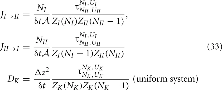
Also the fluxes from slab I to slab II and the reverse can be expressed by the transition probabilities P(I → II) and P(II → I). These fluxes measure the number of crossings between the two slabs per unit of time per surface area. Henceforth, these must be proportional to P(I → II) or P(II → I), the chance that a single particle makes the transition within δt, times the number of molecules in the respective slabs or

where = V/Δz is the surface area of the slabs. For the net rate we can write

$\begin{array}{cc}J=J_{I\to II}-J_{II\to I}& (24)\end{array}$

So, in order to express both diffusion and fluxes in terms of microscopic properties, we need to develop microscopic relations to express P(I → II) and P(II → I).

In general, both the number density and the external potential in each slab might differ. Though, within each slab we assume local equilibrium which implies a fast diffusion in the x and y directions and a relatively fast decay of the velocity autocorrelation function along the z-direction. Let N_I and N_II be the number of particles in each slab and let W_I and W_II be the potentials that are felt by these particles in each slab that includes both intra-particle interactions and the effect of a possible external potential. At the microscopic level we can express any possible one-particle I → II transition as a transition between two microstates i and j that belong to two different classes, X ≡ {N_I, N_II − 1} and Y ≡ {N_I − 1, N_II} respectively. The class or macrostate {n, m} refers to the collection of points in phasespace, describing the two slabs as collective system, having n and m particles in each slab. Now, by introducing t(i → j) as the dynamical transition probability to make a physical transition from microstate i to j using a δt timestep, we can write that

$\begin{array}{cc}\begin{array}{l}P(I\to II)={\displaystyle \sum _{i\in X}P}(i|i\in X){\displaystyle \sum _{j\in Y}t}(i\to j)\\ P(II\to I)={\displaystyle \sum _{j\in Y}P}(j|j\in Y){\displaystyle \sum _{i\in X}t}(j\to i)\end{array}& (25)\end{array}$

Using the Boltzmann statistics that says that the equilibrium probability of state i is proportional e^−βU_i with U_i the total energy of microstate i and assuming local equilibrium we can express the conditional probability P(i|i ∈ X) as the equilibrium probability P_eq(i) ∝ e^−βU_i divided by the probability P(X) ∝ ∑_{i′ ∈ X} e ^−βU_i′ of macrostate X. Therefore P(i|i ∈ X) = e^−βU_i/ ∑_{i′ ∈ X} e^−βU_i′, which leads to

$\begin{array}{cc}\begin{array}{l}P(I\to II)=\frac{{\displaystyle {\sum }_{i\in X}{e}^{-\beta U_i}}{\displaystyle {\sum }_{j\in Y}t}(i\to j)}{{\displaystyle {\sum }_{i\in X}{e}^{-\beta U_i}}}\\ P(II\to I)=\frac{{\displaystyle {\sum }_{j\in Y}{e}^{-\beta U_j}}{\displaystyle {\sum }_{i\in X}t}(j\to i)}{{\displaystyle {\sum }_{j\in Y}{e}^{-\beta U_j}}}\end{array}& (26)\end{array}$

Naturally t(i → j) will depend on the details of the dynamics of the system, but it should obey microscopic reversibility

$\begin{array}{ll}\begin{array}{l}{P}_{eq}(i)t(i\to j)=P_{eq}(j)t(j\to i)\Rightarrow \\ e^{-\beta U_i}t(i\to j)=e^{-\beta U_j}t(j\to i)\end{array}& (27)\end{array}$

and therefore we can write

$\begin{array}{cc}{\displaystyle \sum _{i\in X}{\displaystyle \sum _{j\in Y}{e}^{-\beta U_i}}}t(i\to j)={\displaystyle \sum _{i\in X}{\displaystyle \sum _{j\in Y}{e}^{-\beta U_j}}}t(j\to i)& (28)\end{array}$

For further use we will define

$\begin{array}{cc}\begin{array}{l}{\tau }_{N_{II},U_{II}}^{N_I,U_I}={\displaystyle \sum _{i\in X}{\displaystyle \sum _{j\in Y}{e}^{-\beta U_i}}}t(i\to j)\\ ={\displaystyle \sum _{i\in X}{\displaystyle \sum _{j\in Y}{e}^{-\beta U_j}}}t(j\to i)\end{array}& (29)\end{array}$

which obeys the symmetry relation τNI,UINII,UII. = τNII,UII NI,UI.

Here we should reflect upon the microscopic reversibility equation Equation (27) regarding the issue of whether we should consider States i and j to be defined in phase space or configuration space. Both treatments are valid, but for our purpose configuration space is more convenient. Hence U_i in Equations (25) and (27) should be considered as the potential energy. This implies that t(i → j) also includes the probability that configuration state i has the right velocities, both in magnitude and direction, to make the transition i → j possible, in addition to possible stochastic parameters. The relation 27 is therefore valid for a wide range of dynamics ranging from deterministic NVE dynamics, thermostated dynamics like Andersen or Nosé-Hoover, Langevin, and Brownian dynamics. However, it is also a valid remark whether we should consider all transitions. Δz has a finite value, but δt can, in principle, be taken to the limit δt → 0. Therefore, only particles close to the edges can make the transition within a single timestep. Since it takes many timesteps for this particle to diffuse to the middle of the new slab, it might well recross the boundary several times before this happens. These types of correlations can be avoided by only counting the so-called effective crossings [15, 16] (See Figure 1].

FIGURE 1

Figure 1. Illustration of how the counting of diffusive correlations can be avoided using the effective positive flux formalism [15]. The approach is based on the principle that for each trajectory that starts at the middle (point a) of one slab and ends at the middle of neighboring slab (point f) only one crossing should be considered as “effective.” For instance, the last time that it crosses the interface between the slabs (crossing i → j). This implies that the crossings at points b, c, d and e are not considered. For the reverse trajectories, that move from right to left, we should then consider the first crossings of these trajectories. The microscopic reversibility condition, Equation (27), is then still valid since the statistical probability of trajectory (a → b → c → d → e → i → j → f) equals the probability of the reversed path (f → j → i → e → d → c → b → a) in which time order and velocities are reversed [15].

Now, we will assume that the total potential energy U_i and U_j of states i and j, that describe both slabs I and II as a whole, can be written as the sum of energies of the individual slabs. In other words, we assume that, for the calculation of the total energy, we can neglect the interaction between particles that are in different slabs. This implies that

$\begin{array}{cc}\begin{array}{l}{\displaystyle \sum _{i\in X}{e}^{-\beta U_i}}=Z_I(N_I)Z_{II}(N_{II}-1)\\ {\displaystyle \sum _{j\in Y}{e}^{-\beta U_j}}=Z_I(N_I-1)Z_{II}(N_{II})\end{array}& (30)\end{array}$

where we introduced the partition function integrals Z_K(N)

$\begin{array}{cc}{Z}_K(N)={\displaystyle \int \text{d}}{\text{R}}^N{e}^{-\beta W_K({\text{R}}^N)}& (31)\end{array}$

Hence,

$\begin{array}{cc}\begin{array}{l}P(I\to II)=\frac{{\tau }_{N_{II},U_{II}}^{N_I,U_I}}{Z_I(N_I)Z_{II}(N_{II}-1)},\\ P(II\to I)=\frac{{\tau }_{N_{II},U_{II}}^{N_I,U_I}}{Z_I(N_I-1)Z_{II}(N_{II})}\end{array}& (32)\end{array}$

We can now substitute these expressions into the earlier derived expressions for the flux and diffusion coefficient:

Though, for a non-uniform system the diffusion coefficient is, in principle, not exactly defined. In fact, the transition probability to jump to the right might differ from to the transition probability to jump the left. We will show that, if we define the diffusion coefficient in the middle of two slabs as the geometric mean of these two possibilities

$\begin{array}{cc}\begin{array}{l}{D}_{I,II}=\frac{\Delta z^2}{\delta t}\sqrt{P(I\to II)P(II\to I)}(\text{non-uniform})\\ =\frac{\Delta z^2}{\delta t}\frac{{\tau }_{N_{II},U_{II}}^{N_I,U_I}}{\sqrt{Z_I(N_I)Z_{II}(N_{II}-1)Z_I(N_I-1)Z_{II}(N_{II})}},\end{array}& (34)\end{array}$

we can reobtain the diffusion equation, Equation (6). For this purpose, we also need to define the activity coefficient at the interface. Using the partition function integral 15, we get simple expressions for the activities, Equation (15), and activity coefficients

$\begin{array}{cc}\begin{array}{l}{a}_K=v^{*}\frac{N_K{Z}_K(N_K-1)}{Z_K(N_K)},\\ {\gamma }_K=a_K/C=v^{*}V\frac{Z_K(N_K-1)}{Z_K(N_K)}\end{array}& (35)\end{array}$

Now, similar to Equation (34), we will also use the geometric mean to define the activity coefficient of the intermediate region between two slabs

$\begin{array}{cc}{\gamma }_{I,II}=\sqrt{{\gamma }_I{\gamma }_{II}}=v^{*}V\sqrt{\frac{Z_I(N_I-1)Z_{II}(N_{II}-1)}{Z_I(N_I)Z_{II}(N_{II})}}& (36)\end{array}$

With these definitions at hand, we can derive a neat expression for the net rate

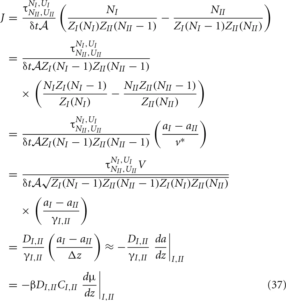
Hence, we reobtained the general diffusion equation Equation (6) from microscopic principles. In the last line we used βμ = ln a + const. ⇒ Cβdμ/dz = (C/a)da/dz = (1/γ)da/dz. In retrospect, this also justifies the use of the geometric mean instead of a normal average to express the diffusion coefficient and activity coefficient at the interface of two slabs. We will use these definitions, Equations. (34) and (36), in the following two sections to analyze the possible density dependence of k′_a and k′_d of Equation (4).

4.2. Activity Based Flux Expression

Based on the diffusion equation 6 we can derive the activity based flux expression 10. The derivation given here is slightly different from the one given in Kjelstrup et al [13]. Instead of using expression 6 we use the one-but-last expression of 37 that is equivalent

$\begin{array}{cc}J(z,t)=-\frac{D(z,t)}{\gamma (z,t)}\frac{da(z,t)}{dz}& (38)\end{array}$

Using the steady state approximation, we can assume that after a short initialization the flux no longer depends on position.

$\begin{array}{cc}\begin{array}{l}\text{for }t>t_{init}\text{ and }z\in \text{barrier region}:\\ J\text{(}z\text{, }t\text{) = }J\text{(}t\text{)}\end{array}& (39)\end{array}$

Now, we can divide Equation (38) by D/γ and integrate both expressions at either side of the equals sign from z = z_R to z = z_P with z_R and z_P being the reactant state and product state values for the reaction coordinate.

$\begin{array}{cc}\begin{array}{l}{\displaystyle {\int }_{z_R}^{z_P}\frac{J(t)\gamma (z,t)}{D(z,t)}}dz=-{\displaystyle {\int }_{z_R}^{z_P}\frac{da(z,t)}{dz}}dz\Rightarrow \\ J(t)={\left[{\displaystyle {\int }_{z_R}^{z_P}\left(\frac{\gamma (z,t)}{D(z,t)}\right)}\text{d}z\right]}^{-1}\left(a(z_R,t)-a(z_P,t)\right)\end{array}& (40)\end{array}$

The largest contribution to the integral is generally around the transition state. Since the transition state is generally a state of low density, in many cases the ideal gas law applies to this region which gives an activity coefficient γ(z_TS) ∝ e^βU_TS with U_TS the potential barrier that each molecule acquires when it is at the transition state [See also Equation (A17) of the appendix]. In addition, the fact that the transition state has a low density during the complete course of the reaction, also little variations in the diffusion coefficient are expected: D(z_TS,t) ≈ D_TS. Under these circumstances the integral becomes independent of time

$\begin{array}{cc}{\displaystyle {\int }_{z_R}^{z_P}\left(\frac{\gamma (z,t)}{D(z,t)}\right)}dz\approx A\left(\frac{e^{\beta U_{\text{TS}}}}{D^{TS}}\right)& (41)\end{array}$

where A is a frequency factor related to the curvature of the potential barrier at the transition state. We will come back to Equation (41) later on. As we will show, it is exactly this approximation that fails in the case of surface adsorption and, therefore, explains the contradiction between Equation (2) and 4.

Finally, we will have to take care for the fact that activities of different phases are generally defined using different reference states. Hence, instead of v* = exp(−βμ°)Λ³ we should use the appropriate values v_R = exp(−βμ°_R)Λ³ and v_P = exp(−βμ°_P)Λ³ that are used for the reactant and product state which implies

$\begin{array}{cc}\begin{array}{l}{a}_R(t)=\frac{a(z_R,t)}{v^{*}}\exp (-\beta {\mu }_R^{°}{\Lambda }^3),\\ a_P(t)=\frac{a(z_P,t)}{v^{*}}\exp (-\beta {\mu }_P^{°}{\Lambda }^3)\end{array}& (42)\end{array}$

which finally gives the result of Equation (7): J = k_f a_R − k_r a_P, with constants

$\begin{array}{cc}\begin{array}{l}{k}_f=\left(\frac{v^{*}{D}_{TS}{e}^{\beta {\mu }_R^{°}}}{A}\right)e^{-\beta U_{\text{TS}}},\\ k_r=\left(\frac{v^{*}{D}_{TS}{e}^{\beta {\mu }_P^{°}}}{A}\right)e^{-\beta U_{\text{TS}}},\end{array}& (43)\end{array}$

and the ratio k_f/k_b corresponds to Equation (9). Splitting the forward and backward part and setting a_R = a_ads. and a_P = a_gas results in Equation (10).

In the appendix we show how this works for simple three-level system. An important lesson from that analysis is that the theoretical forward rate k_fa_R and backward rates k_ra_P are indeed the uncorrelated fluxes. Henceforth, despite that the mathematical derivation involves quite a lot operations with the sole aim to get expressions for the net rate rather than the separate forward or back rates, the theoretical expressions for J_f and J_r should, in principle, reflect the same fluxes as the ones considered in kinetic models. However, the only microscopic term that is really of dynamical nature are the t(i → j) transition probabilities and everything that depends on these. Therefore, all dynamical properties in the thermodynamic rate equation are somehow adsorbed in the diffusion coefficient D. As we will see, the apparent contradiction between kinetic and thermodynamic rate theory is due to the fact that k_f and k_b are in fact not constants but depending on θ because the the approximation given in Equation (41) is invalid for adsorption processes.

5. Diffusion and Activity Coefficients at the Adsorbent-Gas Interface

As stated in the previous section, the key assumption that determines the validity of the thermodynamic rate equations (Equation 10) is the approximation of Equation (41). In order to address the validity of Equation (41) for surface adsorption, we need to determine the activity and diffusion coefficient in the whole system, i.e., also on the boundary of the gas-solid interface. For this, we will use the definitions given by Equations (34) and (36).

First, we need to derive an expression for τNads., Uads. Ngas,Ugas that is given by Equation (29)

$\begin{array}{cc}\begin{array}{l}{\tau }_{N_{\text{gas}},U_{\text{gas}}}^{N_{\text{ads}.},U_{\text{ads}.}}={\displaystyle \sum _{i\in X}{\displaystyle \sum _{j\in Y}{e}^{-\beta U_i}}}t(i\to j)\\ ={\displaystyle \sum _{i\in X}{\displaystyle \sum _{j\in Y}{e}^{-\beta U_j}}}t(j\to i)\end{array}& (44)\end{array}$

where X and Y are descriptions of a state consisting of two layers; an adsorbent layer in contact with a layer of gas, X having {N_ads., N_gas − 1} and Y having {N_ads. − 1, N_gas} molecules in either phase. Now, it is most convenient to use the first expression that includes t(i → j) and assume that for each i ∈ X there is a fixed number of states j ∈ Y with non-zero transition probability t(i → j) with j being a state that is almost identical to state i except for the z coordinate of the target particle. Then, by stating that ∑_j t(i → j) is a constant equal to k′δt we get

$\begin{array}{cc}\begin{array}{l}{\tau }_{N_{\text{gas}},U_{\text{gas}}}^{N_{\text{ads}.},U_{\text{ads}.}}={\displaystyle \sum _{i\in X}{e}^{-\beta U_i}}{k}^{\prime }\delta t\\ =Z_{\text{ads}.}(N_{\text{ads}.})Z_{\text{gas}}(N_{\text{gas}}-1)k^{\prime }\delta t\end{array}& (45)\end{array}$

and for the diffusion coefficient

$\begin{array}{cc}\begin{array}{l}{D}_{\text{gas},\text{ads}.}=\Delta z^2{k}^{\prime }\sqrt{\frac{Z_{\text{ads}.}(N_{\text{ads}.})Z_{\text{gas}}(N_{\text{gas}}-1)}{Z_{\text{ads}.}(N_{\text{ads}.}-1)Z_{\text{gas}}(N_{\text{gas}})}}\\ =\Delta z^2{k}^{\prime }\sqrt{e^{\beta \left|u_a\right|}{V}_{\text{vac}}(M_{\text{vac}}-N_{\text{ads}.})\frac{1}{V}}\\ =\Delta z^2{k}^{\prime }\sqrt{e^{\beta \left|u_a\right|}{C}_{\text{site}}{V}_{\text{vac}}(1-\theta )}\end{array}& (46)\end{array}$

where we used again Equation (16), θ = N_ads./M_vac, and C_site = M_vac/V. As a result, we have obtained the interesting conclusion that the diffusion constant depends on the coverage as ∝ $\sqrt{1-\theta }$.

The activity coefficient at the interface follows directly from ${\gamma }_{\text{gas},\text{ads}.}=\sqrt{{\gamma }_{\text{gas}}{\gamma }_{\text{ads}.}}$ and Equations (17)

$\begin{array}{cc}{\gamma }_{\text{gas},\text{ads}.}=v^{*}\sqrt{\frac{e^{-\beta \left|u_a\right|}}{V_{\text{vac}}{C}_{\text{site}}(1-\theta )}}& (47)\end{array}$

and hence

$\begin{array}{cc}\frac{D_{\text{gas},\text{ads}.}}{{\gamma }_{\text{gas},\text{ads}.}}=\frac{\Delta z^2{k}^{\prime }}{v^{*}}{e}^{\beta \left|u_a\right|}{V}_{\text{vac}}{C}_{\text{site}}(1-\theta )& (48)\end{array}$

Let us now consider Equation (40) for the adsorption process

$\begin{array}{cc}\begin{array}{l}J/(a_{\text{gas}}-a_{\text{ads}.})={\left[{\displaystyle {\int }_{z_{\text{gas}}}^{z_{\text{ads}.}}\left(\frac{\gamma (z,t)}{D(z,t)}\right)}dz\right]}^{-1}\\ \approx {\left[{\left(\frac{D_{\text{gas},\text{ads}.}}{{\gamma }_{\text{gas},\text{ads}.}}\right)}^{-1}\Delta z+{\left(\frac{D_{\text{gas}}}{{\gamma }_{\text{gas}}}\right)}^{-1}|z_{\text{gas}}-z_{\text{ads}.}-\Delta z|\right]}^{-1}\end{array}& (49)\end{array}$

This relation is in fact not completely valid since we cannot assume steady state behavior (position independent flux) in the gas phase z ∈ [z_ads. + Δz : z_gas] where the potential is flat. Still it is useful to consider the above equation qualitatively. It shows that for low coverage the system might well behave like the thermodynamic rate equation which implies that the fluxes are proportional to activities. The fluxes mainly depend on the diffusion coefficient in the gas phase. However, when the coverage increases the (D_gas,ads./γ_gas,ads.)⁻¹ always becomes dominant since it grows as 1/(1 − θ).

Since the kinetic models consider simply the fluxes between one phase to the other, we will just consider the fluxes between two layers, one layer of gas and one layer describing the adsorbed state. In other words |z_gas − z_ads.| = Δz and therefore

$\begin{array}{cc}J=\left(\frac{D_{\text{gas},\text{ads}.}}{{\gamma }_{\text{gas},\text{ads}.}\Delta z}\right)(a_{\text{gas}}-a_{\text{ads}.})& (50)\end{array}$

This implies that for surface adsorption k_f = k_r = (D_gas,ads./γ_gas,ads. Δz) in Equation (10) and these are not constant but depend on the coverage θ. The generalized equilibrium constant K is unity; since the hydrogens do not dissociate or undergo another type of chemical reaction, we use the same reference chemical potential for product and reactant in Equation (9). Substitution of the activities of Equations (17) yields the “constants” of Equation (4) as

$\begin{array}{cc}\begin{array}{l}{k^{\prime }}_a=\frac{D_{\text{gas},\text{ads}.}}{{\gamma }_{\text{gas},\text{ads}.}\Delta z}{v}^{*}\beta \\ {k^{\prime }}_d=\frac{D_{\text{gas},\text{ads}.}}{{\gamma }_{\text{gas},\text{ads}.}\Delta z}\frac{v^{*}\exp (-\beta |u_a|)}{V_{\text{vac}}}\end{array}& (51)\end{array}$

or after substitution of Equation (48)

$\begin{array}{cc}\begin{array}{l}{k^{\prime }}_a=\Delta z{k}^{\prime }{e}^{\beta \left|u_a\right|}{V}_{\text{vac}}{C}_{\text{site}}(1-\theta )\beta \\ {k^{\prime }}_d=\Delta z{k}^{\prime }{C}_{\text{site}}(1-\theta )\end{array}& (52)\end{array}$

This shows that since D_gas,ads. ∝ $\sqrt{1-\theta }$ and γ_gas,ads. ∝ 1/$\sqrt{1-\theta }$ the 1/(1 − θ) dependence of a_ads. is exactly cancelled while the missing (1 − θ) dependence of the adsorption flux is exactly compensated. In fact, J_a = k′_aP and J_d = k′_d θ/(1 − θ) is identical to the Langmuir equations Equations (2), J_a = k_aP (1 − θ), J_d = k_d θ with

$\begin{array}{cc}\begin{array}{l}{k}_a=\Delta z{k}^{\prime }{C}_{\text{site}}\beta e^{\beta \left|u_a\right|}{V}_{\text{vac}}\\ k_d=\Delta z{k}^{\prime }{C}_{\text{site}}\end{array}& (53)\end{array}$

Moreover, k_a/k_d = βV_vace^β|u_a| which is in agreement with Equation (18). The notion that the Langmuir equations do not automatically follow from the standard non-equilibrium thermodynamics approach has been made before by Pagonabarraga and Rubí in Pagonabarraga and Rubi [14]. They state that non-linear relations between fluxes and forces are indispensable to derive the Langmuir equation from thermodynamic rate theory. We are the first to derive these relations from microscopic principles and show that this non-linearity is related to the diffusion and activity coefficients at the solid gas interface for which we can give exact expressions.

6. Correlated Fluxes

We derived that the thermodynamic rate equations and kinetic rate equations are consistent if the right expressions for diffusion and activity coefficients are used. This has the implication that the thermodynamic rate constants are in fact not constant for the cases in which the diffusion and activity coefficients depend on the densities. And in fact, this is exactly the case for a system that behaves according to the Langmuir model. However, we still need to explain the results of Simon et al. [11] who found that kinetic data of hydrogen adsorption simulations agreed with thermodynamic rate equations in which fluxes are simply proportional to activities, i.e., with constants being truly constant.

We will reason that measured fluxes contain the reactive flux (which is approximately Langmuirian) but also correlated fluxes. These are basically the particles that approach the adsorbent sufficiently close at a spot that is already occupied by another molecule. Therefore, this particle is repelled back almost instantly into the gas. If we just count all events in which molecules cross a certain threshold distance away from the adsorbent, this process would be considered as adsorption followed by an immediate desorption. Although this is a valid way to measure the net flux (where these processes cancel), we should disregard these correlated events in our theoretical analysis since these do not contribute to the rate of an reaction nor to the diffusion.

Now, we will decompose the fluxes for adsorption and desorption that are just based on the distance and not corrected for correlations J^dist._a and J^dist._d, into two components: the Langmuir-flux and the correlated-flux

$\begin{array}{cc}{J}_a^{\text{dist}.}=J_a^L+J_a^c,J_d^{\text{dist}.}=J_d^L+J_d^c& (54)\end{array}$

Since each correlated adsorption is directly followed by a desorption, we can write J^c_a = J^c_d = J^c. We can assume that these bounce-back events occur with a frequency that is proportional to the fraction of occupied sites and the pressure.

$\begin{array}{cc}{J}^c={\widehat{k}}_{a}P\theta & (55)\end{array}$

Now, if we take ${\widehat{k}}_a$ = k_a we reobtain the expression for J_a in Equation (4)

$\begin{array}{cc}{J}_a^{\text{dist}.}=J_a^L+J^c=k_{a}P(1-\theta )+k_{a}P\theta =k_{a}P& (56)\end{array}$

and for the desorption we can write

$\begin{array}{cc}{J}_d^{\text{dist}.}=J_d^L+J^c=k_d\theta +k_{a}P\theta ,& (57)\end{array}$

which still looks rather different from Equation (4). However, since Langmuir statistics is conserved, we can simply invert Equation (3) to get pressure as function of θ:

$\begin{array}{cc}P=\frac{\theta }{\frac{k_a}{k_d}(1-\theta )}& (58)\end{array}$

Substitution of this expression into Equation (57) gives

$\begin{array}{cc}{J}_d^{\text{dist}.}=k_d\theta +k_a\frac{{\theta }^2}{\frac{k_a}{k_d}(1-\theta )}=\frac{k_d\theta }{1-\theta }& (59)\end{array}$

which exactly agrees with the simulation data of Simon et al. [11] and thermodynamic rate theory, Equation (4), with the (false) assumption that k_f and k_r are constants.

Often, there is a large separation in timescales which makes it easy to distinguish between correlated or uncorrelated events. However, there are also cases where this is less obvious. In the next section, we will apply a correlated-flux analysis on the simulation data of Simon et al. [11] based on the residence time at the surface.

7. Hydrogen on Graphite

Finally, we come back to the results of Simon et al. [11] and show that the main disagreement between Langmuir kinetics and the fluxes measured in the simulations is due to the counting of correlated data. We repeated the simulations of Simon et al. [11] using the same parameters. 1 ns NVE simulations consisting of 100, 200, 300, 350, 400, 450, 500, 550, 600, 650, and 700 hydrogen molecules were simulated at an average kinetic energy corresponding to temperature of T = 180 K. The isotherm is given in Figure 2 and shows that it is reasonably well described by the Langmuir model where the surface density equals C_ads.(P) = C_maxθ(P) = C_maxαP/(1 + αP) with C_max being the maximum surface density and α = k_a/k_d. The fitted Langmuir parameters are C_max = 0.034 mmol/m² and α = 0.013. The maximum surface density is somewhat larger than the one reported by Simon et al. [11] (≈ 0.015 at 180 K). This might be the effect of small differences in the simulation set-up. Simon et al. used a smaller simulation box which might lead to larger finite size effects. More significant is probably the flexible graphite surface that was used in Simon et al. [11] whereas we adopted a fixed graphite surface. On the other hand, the pressure range in both studies is still very much inside the linear regime of the adsorption isotherm which make it difficult to fit accurately C_max (see bottom-right corner of Figure 2]. However, the most important conclusion is that the Langmuir model can be fitted to our data, just like the results of Simon et al. [11].

FIGURE 2

Figure 2. Isotherm (red) with corresponding Langmuir fit (green). The inset in the top-left corner shows 1/C_ads.(P) vs 1/P which should be linear for Langmuirian types of isotherms: (1/C_ads.(P)) = (1/C_maxα) (1/P) + (1/C_max). Langmuir parameters were obtained from the slope and intersection of the linear fit. The bottom-right corner shows an extrapolation of the fitted curve at a larger pressure domain.

In Figure 3 (red line) we show the flux using the same counting strategy of Simon et al. [11]. This implies that a hydrogen is considered adsorbed when it is within 3 Å of the surface. The flux is, hence, measured by counting the molecules crossing the z = 3 Å line. The desorption and adsorption fluxes are equal since we consider a system in equilibrium in which the net flux is zero, but the individual desorption/adsorption flux increases linearly as function of pressure and faster than linearly as function of coverage θ. As argued in previous section, this behavior might be due to correlations that correspond to events that do not settle but are repelled back to the gas phase. In order to quantify the fraction of correlated crossings we examined the distribution of residence times on the surface after an adsorption event. In the case of ideal two-state kinetics, this distribution should be simple exponential P(t) ∝ exp(−kt) with k being the rate constant. In the presence of correlations, we expect the distribution to be a superposition of the ideal distribution and a distribution that is peaked at the small t. Therefore, we assume that we can model this overall time distribution as

$\begin{array}{cc}P(t)=q_1{e}^{-k_{1}t}+q_2{e}^{-k_{2}t}\text{with}{k}_1\gg k_2& (60)\end{array}$

$\begin{array}{cc}{\displaystyle {\int }_0^{\infty }P}(t)dt=1\Rightarrow q_1=\frac{k_1}{k_2}(k_2-q_2),& (61)\end{array}$

where we used the fact that the distribution is normalized. From an accurate estimation of P(t) it is relatively easy to fit k₁, k₂ and q₂ since in a log(P(t)) vs. t two straight lines should be visible; a first line at small t with slope −k₁ and a second with slope −k₂. The determination of P(t) is technically a little problematic since it requires to set up bins of finite width describing small time-intervals and creating a histogram by counting the number of residence times for each bin. However, taking a too small bin-size results into spikes since many bins will contain no points at all. Too large bins will result in a graph having a huge first block that contain all correlated crossings and is therefore not so informative. One could think of setting up bins of variable length, but our solution is more convenient. Instead of computing P(t) we compute the integral

$\begin{array}{cc}T(t)\equiv 1-{\displaystyle {\int }_0^{t}P}(t)\text{d}t\approx \frac{q_1}{k_1}{e}^{-k_{1}t}+\frac{q_2}{k_2}{e}^{-k_{2}t}& (62)\end{array}$

The construction of T(t) is much less sensitive to the bin-size similar to the construction of a crossing probability [17]. In Figure 4 we constructed the histogram for T(t) using a bin size of 0.2 ps and the plot looks smooth upto at least 60 ps. The parameters k₂ and q₂ are directly obtained by the slope and intersection of a straight line fitted to the linear part (10 ps < t <30 ps) in the log plot. After subtracting this exponential function q₂ exp(−k₂t)/k₂ from the histogram T(t), the remaining part can be fitted again at the small timescale to obtain k₁. In Figure 4 we show the graph T(t) obtained from simulations together with the fit. The insets of Figure 4 show the non-integrated time distribution P(t) both in normal-scale and in log-scale together with the fitted double exponential that was obtained from the integrated curve. The two timescales corresponding to correlated and uncorrelated adsorbing events are clearly visible, though they are not completely non-overlapping. Therefore, taking a fixed time, say 5 ps, and assuming that all crossings that remain a shorter time on the surface should be considered as a correlated crossing, won't work very well. Even a significant part of the uncorrelated distribution q₂ exp(−k₂t) is on this short timescale. In our approach we get a better separation between correlated and uncorrelated crossings when the timescale k⁻¹₁ and k⁻¹₂ are still within one order of magnitude. The fraction of correlations can also be obtained as (k₂ − q₂)/k₂ which increases more or less linearly with increasing coverage just as expected (see Figure 5]. We can repeat the same analysis on the residence time in the gas phase. Surprisingly, that analysis shows an even stronger separation and a fraction of correlations that is around 80%. The reason for this is that the distance z = 3 Å is still very much inside the potential of attraction. Hence, many particles crossing this line from the adsorbed phase have not enough energy to really escape and quickly fall back to the surface. The fraction of these short time recrossings is therefore more or less constant, independent of coverage and pressure. In fact, it is following an opposite trend with a small decrease in the number of correlations. In our analysis we do not correct for these recrossings. Hence, crossing the z = 3 Å from the lower distance is assumed to be a successful transition to the gas phase. This way of counting makes a consistent story with the Langmuir kinetic model. The calculation of the population correlation function [18, 19] would be a way to account for the multiple correlation events, but that is not the aim of this article. What is important is that k₂ corresponds to the frequency that particles coming from the gas phase become long-lived surface particles. If multiplied with the average number of surface particles, this gives the uncorrelated flux that must be the same for desorption and adsorption. Figure 3 also shows the uncorrelated flux that goes to a constant for increasing pressure which is in agreement with Langmuir kinetics. When considered as function of coverage, the flux is increasing a bit less than linear due to a k₂ that is somewhat smaller at the higher pressures. This is also not illogical since the gas is not an ideal gas. Particles from it will collide with surface atoms that try to escape from surface but are then kicked back without crossing the z = 3 Å line. Hence, our results suggest that the biggest approximation of the Langmuir model for this system lies in the treatment of the gas phase as an ideal gas rather than the neglect of repulsions between adsorbed molecules.

FIGURE 3

Figure 3. Absolute flux and the flux corrected for correlations.

FIGURE 4

Figure 4. Residence time analysis for the hydrogen adsorption system with 700 hydrogen molecules. This system corresponds to a gas pressure of 89 bar. The insets shows the probability distribution of the residence times that the hydrogens spend on the surface. The main panel shows the integrated curve, Equation (62), that was used to fit the double exponential which are, for this pressure, k₁ = 1.37 and k₂ = 0.106 ps⁻¹.

FIGURE 5

Figure 5. Fraction of correlations against coverage.

8. Conclusions

We have shown that apparent discrepancies between kinetic models and thermodynamic rate models for the description of surface sorption is related to the microscopic definition for the diffusion and activity coefficient at the interface between the gas phase and adsorbed phase. We show that the diffusion coefficient D and the activity coefficient γ depend on the coverage θ of the adsorbent: D ∝ $\sqrt{1-\theta }$ and γ ∝ 1/$\sqrt{1-\theta }$. If the proper expressions are applied in the thermodynamic rate equations for the adsorption and desorption fluxes, these are no longer linearly proportional to the activities. The “constants” that are the proportionality coefficients between the sorption fluxes and corresponding activities depend on D and γ and are, therefore, also dependent on the coverage θ. The resulting equations are identical to the ones derived from kinetic principles. We also analyzed molecular simulation data that showed Langmuirian isotherms, but with adsorption and desorption fluxes that were proportional to the activities of each phase, in agreement with thermodynamic rate theory with constant D and γ. We have interpreted these results by making a distinction between correlated fluxes and uncorrelated fluxes. A molecule approaching the surface might discover that the site on the surface is already occupied after which it is bounced back into the gas phase. This can be counted as an extra adsorption event followed by an extra desorption event. By eliminating the excess of events which have a too short residence time on the surface, one can correct for these correlated recrossings. The final corrected data are more consistent with Langmuir kinetics. Elimination of correlated recrossings is also essential for mapping the microscopic full-atom system on more mesoscopic or macroscopic descriptions in which the dynamics are fully described by diffusion coefficients and rate constants.

The results presented in this article are useful since they connect two classes of theories that so far have been used by different groups independently, sometimes leading to contradicting results. Our approach shows how thermodynamic rate theory can be used when the gradient of the chemical potential is difficult to evaluate due to discontinuities or when the diffusion coefficient is physically not clearly defined. By doing so, the thermodynamic rate theory becomes identical to Langmuir kinetics if the system behaves as an ideal Langmuir model. In addition, it allows to derive more general flux and rate equations since the use of chemical potentials can correct for the non-ideality of matter. For instance, we showed that the adsorption fluxes are not simply proportional to the activities (J_a ∝ a_gas, J_d ∝ a_ads.) but proportional to a more complex expression: J_a ∝ (D_gas,ads./γ_gas,ads.)a_gas, J_d ∝ (D_gas,ads./γ_gas,ads.)a_ads. where D_gas,ads. and γ_gas,ads. can in principle depend on both surface coverage and gas pressure. This makes it possible to use thermodynamic rate theory for the modeling of transport and chemical reactions in complex systems which are not well described by the Langmuir kinetics.

Conflict of Interest Statement

The authors declare that the research was conducted in the absence of any commercial or financial relationships that could be construed as a potential conflict of interest.

Acknowledgments

We thank the Research Council of Norway and the Faculty of Natural Sciences and Technology (NTNU) for support via the institution-based strategic projects (ISP): From molecules to process application.

References

1. Zhdanov VP. Adsorption-desorption kinetics and chemical potential of adsorbed and gas-phase particles. J Chem Phys. (2001) 114:4746–8. doi: 10.1063/1.1349178

CrossRef Full Text

2. Ward CA. Liquid-vapour phase change rates and interfacial entropy production. J Non Equilib Thermodyn. (2002) 27:289–303. doi: 10.1515/JNETDY.2002.017

CrossRef Full Text

3. Langmuir I. The adsorption of gases on plane surfaces of glass, mica and platinum. J Am Chem Soc. (1918) 40:1361–403. doi: 10.1021/ja02242a004

CrossRef Full Text

4. Brunauer S, Emmett PH, Teller E. Adsorption of gases in multimolecular layers. J Am Chem Soc. (1938) 60:309–19. doi: 10.1021/ja01269a023

Pubmed Abstract | Pubmed Full Text | CrossRef Full Text

5. Keil T. A statistical derivation of the bet equation. J Chem Phys. (1954) 22:1617–8. doi: 10.1063/1.1740480

CrossRef Full Text

6. Ward CA, Findlay RD, Rizk M. Statistical rate theory of interfacial transport.1. theoretical development. J Chem Phys. (1982) 76:5599–605. doi: 10.1063/1.442865

CrossRef Full Text

7. Kreuzer HJ. Thermal-desorption kinetics. Langmuir (1992) 8:774–81. doi: 10.1021/la00039a009

CrossRef Full Text

8. Payne SH, Kreuzer HJ. Analysis of thermal-desorption data. Surf Sci. 1989 222:404–29. doi: 10.1016/0039-6028(89)90369-5

CrossRef Full Text

9. Kreuzer HJ, Payne SH. Nonequilibrium thermodynamics of a 2-phase adsorbate. Surf Sci. (1988) 198:235–62. doi: 10.1016/0039-6028(88)90482-7

CrossRef Full Text

10. Ho YS, Ng JCY, McKay G. Kinetics of pollutant sorption by biosorbents: review. Sep Purif Methods. (2000) 29:189–232. doi: 10.1081/SPM-100100009

Pubmed Abstract | Pubmed Full Text | CrossRef Full Text

11. Simon JM, Haas OE, Kjelstrup S. Adsorption and desorption of H2 on graphite by molecular dynamics simulations. J Phys Chem. (2010) 114:10212–20. doi: 10.1021/jp1011022

Pubmed Abstract | Pubmed Full Text | CrossRef Full Text

12. de Groot SR, Mazur P. Non-Equilibrium Thermodynamics. New York: Dover (1984).

13. Kjelstrup S, Bedeaux D, Johannessen E. Non-equilibrium Thermodynamics for Engineers. Science and culture series (Singapore): Physics. World Scientific; (2010). Available online at: http://books.google.no/books?id=U3VaEONIDv0C.

14. Pagonabarraga I, Rubí JM. Derivation of the Langmuir adsorption equation from non-equilibrium thermodynamics. Physica A (1992) 188:553–67. doi: 10.1016/0378-4371(92)90331-J

CrossRef Full Text

15. van Erp TS, Bolhuis PG. Elaborating transition interface sampling methods. J Comput Phys. (2005) 205:157–81. doi: 10.1016/j.jcp.2004.11.003

CrossRef Full Text

16. van Erp TS. Dynamical Rare event simulation techniques for equilibrium and non-equilibrium systems. Adv Chem Phys. (2012) 151:27. doi: 10.1002/9781118309513.ch2

CrossRef Full Text

17. van Erp TS, Moroni D, Bolhuis PG. A Novel path sampling method for the sampling of rate constants. J Chem Phys. (2003) 118:7762–74. doi: 10.1063/1.1562614

CrossRef Full Text

18. Chandler D. Introduction to Modern Statistical Mechanics. New York: Oxford University Press (1987).

19. Frenkel D, Smit B. Understanding Molecular Simulation, 2nd Edn. San Diego, CA: Academic Press (2002).

20. Moroni D, Bolhuis PG, van Erp TS. Rate constants for diffusive processes by partial path sampling. J Chem Phys. (2004) 120:4055–65. doi: 10.1063/1.1644537

Pubmed Abstract | Pubmed Full Text | CrossRef Full Text

Appendix

To illustrate the thermodynamic rate equation we consider a simple three-level system that is an abstract model for a reaction barrier with an intermediate energy state (See Figure A1). The overall rate constants k₁₃ and k₃₁ are given by [20]

$\begin{array}{cc}\begin{array}{l}{k}_{13}=k_{12}\frac{k_{23}}{k_{21}+k_{23}}=k_{12}{p}_2^{+}\\ k_{31}=k_{31}\frac{k_{21}}{k_{21}+k_{23}}=k_{32}{p}_2^{-}\end{array}& (\text{A}1)\end{array}$

where p⁺₂ = k₂₃/(k₂₁ + k₂₃) and p⁻₂ = k₂₁/(k₂₁ + k₂₃) are the probabilities that, if the system is at the barrier, it will go the right or left side, respectively. The reaction constants are therefore determined by the frequency that the system jumps on the barrier times the probability to fall off at the other side rather than falling back. The fluxes J_{1 → 3} and J_{3 → 1} are, henceforth, simply

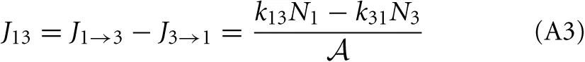
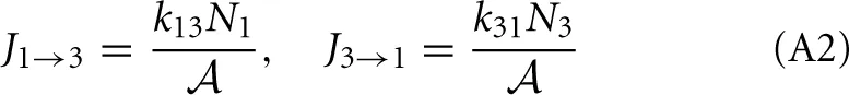and the net flux equals

FIGURE A1

Figure A1. Three-level system: transitions between two low energy states (state 1 and 3) have to pass through an intermediate energy state (state 2) that is higher in energy. k_ij denotes the rate constant from state i to j. The barrier between state 1 and 2 is the transition state and therefore k₂₁ < k₂₃.

Now, let us use thermodynamic rate theory to derive this expression. From Equation (15) we can write down the partition function integral for each each energy state:

$\begin{array}{cc}{Z}_i(N)={\left(V{e}^{-\beta E_i}\right)}^N& (\text{A}4)\end{array}$

and derive the activities and activity coefficients of each level by Equation (35)

$\begin{array}{cc}{a}_i=N_i{e}^{\beta E_i},{\gamma }_i=V{e}^{\beta E_i}& (\text{A}5)\end{array}$

where we have gauged the reference chemical potential μ° = k_BT ln(V/Λ³) so that v*/V = 1. The detailed balance condition implies that

$\begin{array}{cc}{e}^{-\beta E_i}{k}_{i,i+1}=e^{-\beta E_{i+1}}{k}_{i+1,i}& (\text{A}6)\end{array}$

which is independent to the number of particles N_i, N_{i + 1} at each level since we assume non-interacting particles. Moreover, the chance to move to right or left with a time-interval δt is simply given by t(i → i ± 1) = k_{i, i± 1} δt and, therefore, similar to Equation (45)

$\begin{array}{cc}{\tau }_{i,i+1}=Z_i(N_i)Z_{i+1}(N_{i+1}-1)k_{i,i+1}\delta t& (\text{A}7)\end{array}$

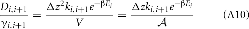
Hence, the diffusion coefficients are (Equation 34)

$\begin{array}{cc}\begin{array}{l}{D}_{i,i+1}=\frac{\Delta z^2}{\delta t}\sqrt{\frac{Z_i(N_i)Z_{i+1}(N_{i+1}-1)}{Z_i(N_i-1)Z_{i+1}(N_{i+1})}}{k}_{i,i+1}\delta t\\ =\Delta z^2\sqrt{k_{i,i+1}{k}_{i+1,i}}\end{array}& (\text{A}8)\end{array}$

The activity coefficient at the boundaries are

$\begin{array}{cc}{\gamma }_{i,i+1}=V\sqrt{\frac{k_{i+1,i}}{k_{i,i+1}}}{e}^{\beta E_i}& (\text{A}9)\end{array}$

So that

Now we can approximate the derivative da/dz

$\begin{array}{cc}\begin{array}{l}\frac{da}{dz}{|}_{i,i+1}\approx \frac{(a_{i+1}-a_i)}{\Delta z}=\frac{1}{\Delta z}\left(e^{\beta E_{i+1}}{N}_{i+1}-e^{\beta E_i}{N}_i\right)\\ =\frac{e^{\beta E_i}}{\Delta z}\left(\frac{k_{i+1,i}{N}_{i+1}-k_{i,i+1}{N}_i)}{k_{i,i+1}}\right)\end{array}& (\text{A}11)\end{array}$

Therefore, the net rate between level 1 and 2 is:

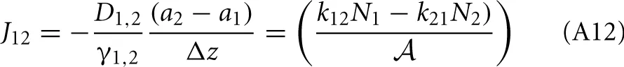
This result is not surprising since it is straightforwardly obtained from a kinetic viewpoint. Though, it shows that thermodynamic rate theory is al least equivalent provided that one uses the right definition for the diffusion and activity coefficients. The net rate between level 2 and 3 follows directly by changing the labels in the equation above

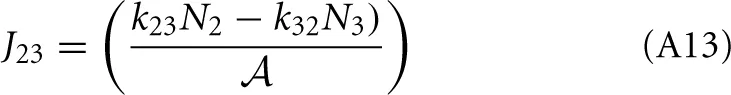
Now, the steady state approximation implies setting dN₂/dt = 0 in the following equation

$\begin{array}{cc}\frac{d{N}_2}{dt}=k_{12}{N}_1+k_{32}{N}_3-k_{21}{N}_2-k_{23}{N}_2\approx 0& (\text{A}14)\end{array}$

which results in

$\begin{array}{cc}{N}_2(t)=\frac{k_{12}{N}_1(t)+k_{32}{N}_3(t)}{k_{21}+k_{23}}& (\text{A}15)\end{array}$

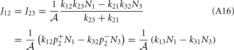
Substitution of this expression into Equations (A12) and (A13) shows that the net rates at the barrier are indeed the same for steady state conditions

and from the integral expression we get

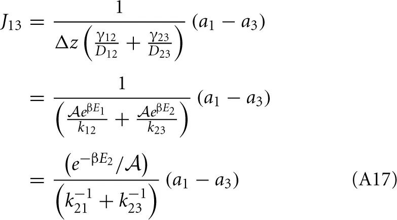where we used e^βE₁/k₁₂ = e^βE₂/k₂₁. The sum k⁻¹₂₁ + k⁻¹₂₃ is mostly determined by the smallest of the two rate constant. For instance if k₂₁ « k₃₂ the thermodynamic rate equations is simply J₁₃ ≈ exp(−βE₂)k₂₁/. In addition, the highest points of the potential barrier, the transition state, is likely to be found between states 1 and 2. This all agrees with Equation (41). Using again the microscopic reversibility relation, we can express activities as

$\begin{array}{cc}{a}_1=N_1\frac{e^{\beta E_2}}{k_{21}}{k}_{12},a_3=N_3\frac{e^{\beta E_2}}{k_{23}}{k}_{32},& (\text{A}18)\end{array}$

which gives

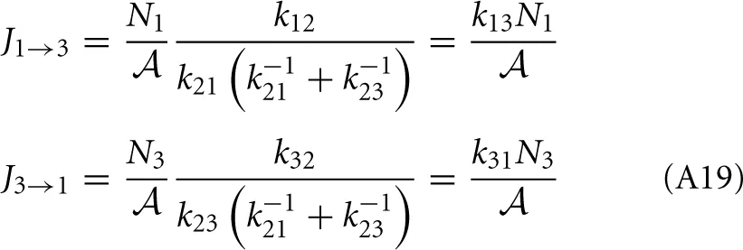
The overall net flux J₁₃ has the same form as J₁₂ or J₂₃ and the kinetic theory based equation, Equation (A3). Another way to express the forward flux is J_{1 → 3} = k_12p2⁺N₁/ = k₁₂ (1 − p⁻₂) N₁/ = J_{1 → 2} − k_12p2⁻N₁/ which is the total flux from state 1 to state 2 minus the correlated flux (crossings that recross the transition state before entering state 3). Hence, it is not that correlated recrossings cancel in the net flux when taking the difference J_{1 → 3} − J_{3 → 1}, but the individual forward and backward fluxes, as obtained from thermodynamic rate theory, are already corrected for fast recrossings.