Nominally brittle cracks in inhomogeneous solids: from microstructural disorder to continuum-level scale

Abstract

We analyze the intermittent dynamics of cracks in heterogeneous brittle materials and the roughness of the resulting fracture surfaces by investigating theoretically and numerically crack propagation in an elastic solid of spatially-distributed toughness. The crack motion splits up into discrete jumps, avalanches, displaying scale-free statistical features characterized by universal exponents. Conversely, the ranges of scales are non-universal and the mean avalanche size and duration depend on the loading microstructure and specimen parameters according to scaling laws which are uncovered. The crack surfaces are found to be logarithmically rough. Their selection by the fracture parameters is formulated in term of scaling laws on the structure functions measured on one-dimensional roughness profiles taken parallel and perpendicular to the direction of crack growth.

1. Introduction

Understanding how solids break continues to pose significant fundamental challenges. For brittle solids broken under tension, Linear Elastic Fracture Mechanics (LEFM) tackles the difficulty by reducing the problem to the destabilization and subsequent growth of a dominant pre-existing crack (see e.g., [1] for an introduction to LEFM). The theory is based on the idea that, in an elastic material, all dissipative and damaging processes are localized in a small zone around the crack tip, so-called fracture process zone, FPZ. Crack destabilization and further motion are then governed by the balance between the flux of mechanical energy released in the FPZ from the surrounding material and the dissipation rate into this zone. The former is computable within linear elasticity theory and connects to the stress intensity factor, which characterizes the near-tip stress field and depends on the external loading and specimen geometry only. The dissipation rate is quantified by the fracture energy required to expose a new unit area of cracked surfaces. Equivalently, it can be quantified by the fracture toughness, i.e., the onset value for the stress intensity factor above which crack starts to grow. Within LEFM theory, both the fracture energy and the fracture toughness are assumed to be material constants, to be measured experimentally.

LEFM framework provides a coherent framework to describe fracture in homogeneous solids. In contrast, heterogeneous solids remain unclear. Stress concentration at the crack tip makes the behavior observed at the continuum-level scale extremely sensitive to material's small scale inhomogeneities. Consequences include crackling dynamics for fracture with discrete pulses (avalanches) of a variety of sizes and erratic crack paths (see [2] for review). A generic observation in this field is the existence of scale free statistics: (i) Direct imaging of the crack motion in paper sheets [3, 4] or along heterogeneous interfaces [5, 6] has revealed power-law distribution for the size of the crack jumps; (ii) the acoustic [7–9] or seismic [10, 11] events going along with fracture are characterized by power-law distribution for the energy; and iii) fracture surfaces are found to exhibit self-affine morphological features [12–16] or logarithmic [17] roughness.

These observations, by essence, cannot be addressed by conventional LEFM continuum approaches. In this context, over the past 25 years, promising alternative approaches have emerged from statistical and non-linear physics: Statistical lattice models like fiber bundle models (see [57] for review) or random fuse models (see [18] for review), for example, were found to reproduce, with a minimal set of ingredients, crackling dynamics in failure [19–21] and self-affine fracture roughness [22–24], in qualitative agreement with some of the experimental observations. However, these approaches remain too minimal to provide quantitative predictions for situations of engineering interests.

A different approach consists in considering the crack propagation in a solid with spatially-distributed toughness. The availability of asymptotic formulas [25–28] for the variations of stress intensity factors along a slightly distorted crack can explicitly take into account the microstructural disorder in a continuum-level scale LEFM-like description [29–32]. Within this framework, referred thereafter to as the Random-Toughness Continuum-Mechanics (RT-CM) approach, the fracture onset can be mapped to a critical depinning transition [2, 33–35]. Depending on the situation, this approach yields logarithmically rough [32] or self-affine [36] fracture surfaces. It can also explain the crackling dynamics sometimes observed as a consequence of a self-adjustment of the driving force around the depinning value [37]. The main advantage here is that the external parameters involved in the depinning model can be mapped to conventional LEFM parameters. This has been used to relate effective toughness and microstructural disorder [38, 39], or to unravel the specific conditions required to observed crackling in brittle fracture [40].

In the present work, depinning models unravel how the loading rate, specimen geometry, and microstructural disorder quantitatively select the statistics of continuum-level scale avalanches (as measured in conventional experimental fracture mechanics) and of the crack roughness (as recorded in conventional fractography). Section 2 presents the derivation of the depinning model from LEFM. This section details the successive assumptions and their implications. Section 3 assesses the statistics of the continuum-level scale avalanches, i.e., bursts evidenced in the time evolution of the spatially-averaged crack velocity. Statistics on the avalanche's size and duration demonstrate a power-law characterized by universal exponents. Conversely, the associated cutoffs do depend on the loading, microstructure, and specimen parameters according to scaling laws which are uncovered. Two regimes can be distinguished: A regime of pseudo-isolated avalanches not so different from what is predicted in the quasi-static limit (vanishing loading rate); and a regime where avalanches coalesce with each other. Section 4 analyzes the statistics of fracture roughness. The structure functions measured along profiles parallel and perpendicular to the direction of crack growth exhibit logarithmic scaling with prefactors and characteristic length-scales depending on the Poisson's ratio and microstructure parameters according to scaling which are uncovered.

2. Materials and methods

In LEFM theory, the crack velocity v is governed by the balance between the mechanical energy G and the (material constant) fracture energy Γ (Griffith criterion). For slow cracks, v/μ = G − Γ where μ = c_R/Γ relates the mobility μ to the Rayleigh wave speed c_R. The principle of local symmetry (PLS) governs the growth direction [41]. This imposes a zero stress intensity factor condition for mode II (K_II = 0) all along the fracture. As consequences, an initially straight crack in an ideal homogeneous material gently loaded in mode I would continuously grow within its plane, without any jerky motion or roughness. But inhomogeneities at the microstructure scale yield distortions of the crack front, which, in turn, induce perturbations δK_I, δK_II, and δK_III in the local loading of the front.

In the RT-CM approach, the effect of material inhomogeneities is taken into account by introducing a random spatially-distributed component for the fracture energy and for the shear part of the loading. Then, Griffith criterion and PLS combined with an asymptotic estimation of the perturbations in the loading induced by the front distortion describes the crack growth. This approach was pioneered by Gao and Rice [29] and subsequently developed [30–32, 37, 40, 42–44]. Here, the model is reviewed with an emphasis on the relation between the model parameters and experimentally measurable quantities. We also pay special attention to list the various assumptions and discuss the implied limits.

2.1. From front distortions to the perturbations in the crack-tip loading

Figure 1

Then, Rice [25] and Movchan et al's [26] formula relate δK_i(z) to the front distortions:

2.2. Griffith criterion and equation of motion

The above expression for the local perturbations δK_i leads to a first order expression of the energy release rate G(z) as a function of the front distortions:

where G₀(t, f) = K₀(t, f)²/E is the reference energy release rate which, as K₀(t, f), would result from the same loading with a straight crack front within the mean plane y = 0 at the mean position x = f(t). Henceforth, the operator a indicates averaging of the variable a(z) over the spatial coordinate z. The two quantities G₀ and K₀ coincide with the ones that would have been defined in the conventional LEFM approach when ignoring front distortions. They only depend on the specimen geometry and imposed load (of which both evolve with t) and can be determined using continuum mechanics (e.g., finite element analysis).

Slow cracking (as considered herein) implies that the solid is loaded by imposing external displacements rather than external stresses (the opposite would yield dynamic fracture with crack at speed on the order of the sound speed). This induces additional constraints: G₀ should decrease with f(t) (specimen compliance always increases with crack length) and increase with t (to drive a crack, external displacement can only increase with time). Without loss of generality, we set t = 0 at a time when the crack has just stopped and x = 0 is the crack tip's position at this time. G₀(t = 0, f = 0) = Γ where Γ = 〈Γ(x, y, z)〉 is the mean value of fracture energy. Considering the subsequent variation f(z, t) to be small with respect to the crack length at t = 0, we can write:

where Ġ = ∂G₀/∂t (driving rate) and G′ = − ∂G₀/∂f (unloading factor) are positive constants characterizing the loading rate and the specimen geometry, respectively. Inserting Equations 1 and 3 in Equation 2, and the resulting expression for G(z) into Griffith criterion, the equation of motion for the in-plane front displacement is:

where γ(x, y, z) = Γ(x, y, z) − Γ is the fluctuating part of the fracture energy. The solution of this equation provides the space-time dynamics of the in-plane projection of the crack front. Subsequently, it gives the time evolution of the fracture velocity at the continuum-level scale, v(t) = df/dt. This is the relevant observable characteristics of the crack dynamics in standard experiments of fracture mechanics.

2.3. Principle of local symmetry and equation of path

We now derive an equation of path by making use of the principle of local symmetry [41]. To do so, we take inspiration from the work of Katzav et al. [44, 47] to model crack path in a model 2D situation and extend it for three-dimensional solids. The idea is to decompose the front propagation along x-axis into infinitesimal straight kinks of length ℓ, identified with the microstructural length-scale characterizing the spatial distribution of Γ(x, y, z) (see Figure 1:right). Consider now the kink occurring at the front location z between time t and t+d t. Leblond et al's formulas [48] relate the stress intensity factors after kinking K′_i(z) (i = I, II, III) to the stress intensity factors before kinking K_i(z) and to the kink angle δθ = θ(z, t + dt) − θ(z, t) = ℓ ∂²h/∂x²(x = f(z, t), z) via:

where F_i,j(δθ) are universal functions that were computed in Leblond [27] for three-dimensional solids. The principle of local symmetry implies that K′_II must be uniformly zero, which leads to:

Now, to first order in δθ, F_{II, I}(δθ) and F_{II, II}(δθ) are given by Leblond [27]: F_{II, I}(δθ) = δθ + O(δθ²) and F_{II, II}(δθ) = 1 + O(δθ²). The kink angle is then related to K₀, δK_I(z) and δK_II(z) via: δθ ≈ −δK_II(z)/(K₀ + δK_I(z)). Finally, by keeping only the first order loading perturbations, it writes:

To introduce the effect of microstructural disorder, a spatially distributed noise term K₀ϑ (x, y, z) is added to the right-handed side of the equation. In the situation of inter-granular crack growth in a material made of sintered grains (e.g. sandstone), for example, this additional term would translate the difference between the kink angle predicted by the principle of local symmetry and that truly selected so that the crack propagates between the cemented grains. Finally, combining the resulting equation with the asymptotic formula for stress intensity factors (Equation 1), one gets:

The solution of this equation provides the topography of the post-mortem fracture surfaces, h(x, z). This is the quantity of interest in fractography science. Note that this equation differs from that given in Larralde [31] and Bonamy et al. [36] as it includes an additional curvature term ∂²h/∂x².

2.4. Relevant parameters and numerical aspects

Note that, in elastic interfaces equations as that proposed in Equations 4 and 8, the scaling properties remain unaffected upon changes in the probability functions (p(γ) and p(ϑ)) and in the correlation functions (C_γ(|r|) and C_ϑ(|r|)) [43]. Thanks to this series of assumptions, the two spatially distributed noise terms are fully characterized with 3 parameters: , and ℓ.

As shown in Ramanathan et al. [32], Equation 8 with a 2D projection for the noise term yields logarithmically smooth fracture surfaces. Hence, zooming out on the fracture surfaces makes them appear flatter and flatter. When the zooming out is sufficient, fluctuations in h become negligible when compared to in-plane length scales. The two noise terms reduce to γ(x, y = h(x, z), z) ≈ γ(x, y = 0, z) and ϑ(x, y = h(x, z), z) ≈ ϑ(x, y = 0, z). This validates Hyp. 8.

At this point, the selection of the fracture behavior brings into play 8 parameters: μ, Γ, Ġ, G′, , , ℓ and W. The introduction of dimensionless time t → t/ℓ/(μΓ) and length {x, y, z, f, h} → {x/ℓ, y/ℓ, z/ℓ, f/ℓ, h/ℓ}) reduces this number. Equations 4 and 8 become:

where the dimensionless noise term η is characterized by a standard deviation = /Γ and a spatial correlation length equal to unity.

The following sections subsequently address the continuum-level scale statistics of crack dynamics v(t) and the morphology of the post-mortem fracture surfaces h(x, z). They also reveal their dependencies on the external parameters {c, k, A, , , N}. The numerical scheme is the following. For each set of parameters, we built two uncorrelated random N × pN maps η(x, z) and ϑ(x, z) with Gaussian distribution of variance and , respectively. At time t = 0, the crack front is a straight line at x = 0: f(z, t = 0) = 0 and h(x = 0, z) = 0 ∀ z ∈ [0, N − 1]. Solving Equation 9a gives the space-time evolution of f(z, t). Solving Equation 9b provides h(x, z). Both cases invoke a fourth order Runge-Kutta scheme and periodic boundary conditions along z: f(z = 0, t) = f(z = N, t) and h(x, z = 0) = h(x, z = N) for all t and x. This speeds up the computation time as the two integral terms in the equations can be solved in the Fourier domain.

3. Results

3.1. Crackling dynamics and avalanche statistics

We first look at the crack dynamics. Equation 9a describes the motion of a long-range elastic chain driven in a frozen random pinning potential with a driving force F = ct − kf(t) self-adjusting around the depinning value [37]. For {c, k} → 0, the chain propagates while remaining at the critical depinning point and the crack moves through irregular jumps, or avalanches. The size S and duration D of the avalanche¹ follow a universal power-law distribution [37, 49]: P(S) ∝ S^−τ and P(D) ∝ D^−α where the exponents τ and α can be estimated using renormalization [49–51] or numerical [52, 53] methods. The most precise estimations yields τ = 1.280 ± 0.01 and α = 1.500 ± 0.010 [2]. These scale free statistics extend to upper cutoffs S₀ and D₀ set by the system size N: S₀ ∝ N^ζ and D₀ ∝ N^κ where ζ and κ are the roughness exponent and dynamic exponent, respectively. The most precise estimations of their value yield [52, 53]: ζ = 0.385 ± 005 and κ = 0.770 ± 0.005.

Here, both c and k are finite. The effects of a finite unloading factor k keeping c → 0 is now fairly well documented [2, 54]: It modifies the upper cutoffs S₀ and D₀ to the preceding scale-free distributions:

Here, the form of the functions f(u) and g(u) is expected to be universal. The exponents 1/σ and 1/Δ are also predicted to be universal: 1/σ = 0.69 ± 0.010 and 1/Δ = 0.385 ± 0.010 [2, 54]. Conversely, the effect of a finite c is not uncovered yet. By yielding some overlap between the avalanches [55], it can significantly alter the dynamics. In particular, a recent work [40] has evidenced a transition line between a crackling-like dynamics made of irregular power-law distributed jumps and a continuum-like dynamics ruled by the conventional LEFM theory.

Figure 2 presents typical times profiles of the continuum-level scale velocity v(t) for different values of c and k in the crackling regime. Here and thereafter, the system size N and the disorder strength are set constant, N = 1024 and = 1, returning at the end of this section to a brief discussion on their effect. Note the irregular jumps characteristics of the underlying avalanching dynamics. Note also the qualitative changes in the signal appearance as k and c are modulated: Pulses become shorter as k increases, and the pulse density increases as c increases. Note finally that, due to the finite value of c, v(t) does not vanish between the pulse, but becomes equal to a small value proportional to c (prefactor dependent of the Runge Kunta scheme). The avalanches are then identified with the bursts where v(t) is above a prescribed reference level v_c = 10⁻³. Their duration D is defined as the interval between the two successive intersections of v(t) with v_c, and their size S is defined as the integral of v(t) − v_c between the same points.

Figure 2

Figure 3 reports the probability density function of avalanche size P(S|c, k) and duration P(D|c, k) for different values of c and k. Power-laws are observed. The exponents τ and α associated with the power-law decrease are independent of c and k. Moreover, they compare well with the values τ = 1.280 ± 0.01 and α = 1.500 ± 0.010 expected for {c, k} → 0. On the other hand, the valid region of the power-law is observed depends on c and k. Both the lower cutoffs S_min and D_min are roughly independent of c and k. However, the precise values S_min and D_min were observed to depend on the reference level v_c and, thus, are to be associated with the procedure to extract the avalanches. We will consider in the following only the part of the distributions above these lower cutoffs.

Figure 3

Direct computation of the cutoff is quite imprecise. Hence, the selection of the typical length and time scales is studied via variations of the mean values 〈S〉(c, k) = ∫^∞_SminS × P(S|c, k)dS (Figure 4A) and 〈D〉 = ∫^∞_DminD × P(D|c, k)dD (Figure 4B). At large enough k, both 〈S〉 and 〈D〉 are independent of c. This large k regime is attributed to a regime of pseudo-isolated (pi) avalanches. The distributions are then expected to take forms similar to that of Equation 10. As a result, 〈S〉^pi is expected [56] to take the form 〈S〉^pi ≈ S^{τ − 1}_minS^{2 − τ}₀ ∝ k^{−(2 − τ)/σ}, 〈D〉^pi ≈ D^{α − 1}_minD^{2 − α}₀ ∝ k^{−(2 − α)/Δ}. These two scaling are compatible with the observations at large k (dash line in Figures 4A,B). As a synthesis, the mean avalanche size and duration are found to take the following form at large k:

Figure 4

Let us try now to characterize the effects of the avalanche overlap when k becomes small or c becomes large. Previous work [40] evidenced a transition between the crackling dynamics studied here and a continuum-like dynamics when c becomes large enough or k small enough. This transition is believed [40] to coincide with the point where the avalanche overlap percolates throughout the entire system. At constant and N, this transition was shown [40] to be fully driven by the ratio c/k. We hence plotted, in Figure 5, 〈S〉/〈S〉^pi and 〈D〉/〈D〉^pi (first order estimation of the number of individual avalanches having merged together to form the bursts detected from the signal v(t)), as a function of the control parameter c/k. A coarse collapse is observed. As expected, the master curves diverge at the transition value between crackling and continuum-like dynamics (materialized by the vertical dash lines in the main panels of Figures 5A,B).

Figure 5

Note that significant deviations to the collapse are observed. They are believed to stem from a qualitative change in the distribution shape as k decreases/c increases and the avalanche overlap increases. Actually, for small k/large c a bump develops at large scales, for both the distribution in size and in duration. Due to this change in shape, several length-scales (resp. time-scales) intervenes in the distributions of S (resp. D). Thus, the recording of the mean values alone is not sufficient to capture their evolutions with c and k. Ongoing work aims at characterizing these effects more accurately.

To make the analysis complete, we looked at the effects of the system size N and disorder strength . Figure 6 plots the probability density function of avalanche size P(S|N, ) and avalanche duration P(D|N, ) as measured for different values of N and at fixed values of c and k. For both size and duration, the decrease of N yields an increase of the lower-cutoffs S_min and D_min (main panel of Figures 6A,A′). The two dependencies are well fitted by power-laws: S_min ∝ N^−a_SN and D_min ∝ N^−a_DN with a_SN ≈ 1.7 and a_DN ≈ 0.6 (inset of Figures 6A,A′). does not seems to affect S_min. Conversely, D_min decreases with as D_min ∝ ^−a_D with a_D ≈ 1.2 (inset of Figure 6B′). The effects of N and of 〈S〉 and 〈D〉 are analyzed in Figure 7, by plotting the curves 〈S〉 vs c and 〈D〉 vs c for different N at constant k and (insets in Figures 7A,A′), and for different at constant k and N (insets in Figures 7B,B′). Increasing N yields a decrease of the low-c plateau and a leftward shift of the divergence location for both 〈S〉 and 〈D〉. Increasing yields an increase of the low-c plateau for 〈S〉, a decrease of the low-c plateau for 〈D〉, and a rightward shift of the divergence location for both 〈S〉 and 〈D〉. All curves can then be superimposed by making {〈S〉 → 〈S〉/N^−b_SN, c → c/N^−c_N} in the main panel of Figure 7A, {〈S〉 → 〈S〉/^b_S, c → c/^c} in the main panel of Figure 7B, {〈D〉 → 〈D〉/N^−b_DN, c → c/N^−c_N} in the main panel of Figure 7A′, {〈D〉 → 〈D〉/^−b_D, c → c/^c} in the main panel of Figure 7B′. By combining this with Equation 11 and the collapse obtained in Figure 5, we anticipate the following form for mean size and duration:

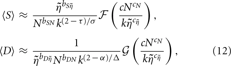
where the two functions (u) and (u) exhibit a plateau at small u, and both diverge at the same value u_c. The value of the exponents τ, α, 1/σ and 1/Δ are well known [2]: They can e.g., be related to the so-called roughness exponent ζ and dynamic exponent κ classically defined in the realm of critical depinning transition: τ = 2 − 1/(1 + ζ), α = 1 + ζ/κ, 1/σ = (1 + ζ)/2 and 1/Δ = κ/(1 + ζ). Conversely, the precise origin of the exponents b_SN, b_S, b_DN, b_D, c_N, and c and their link with ζ and κ remain to be uncovered.

Figure 6

Figure 7

Equation 12 quantitatively relate the material parameters to quantities that are accessible in conventional experimental mechanics, namely the mean size and duration of the avalanches. In this context, it is of interest to rewrites the equation with the original variables, before the non-dimensionalization procedure:

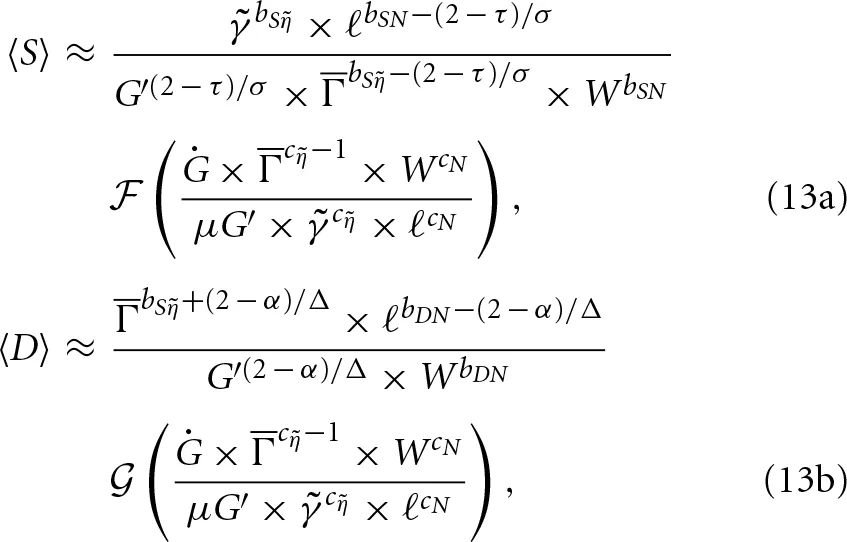
where the mean avalanche size 〈S〉 and duration 〈D〉 are expressed with real length and time units, and Ġ, G′, W, Γ, μ, ℓ and are recalled to be the loading rate, the unloading factor, the specimen width, the fracture energy, the mobility, the microstructure length-scale, and the contrast in local fracture energy. The value of the exponents are recalled to be τ = 1.280 ± 0.01 (predicted), α = 1.500 ± 0.01 (predicted), 1/σ = 0.69 ± 0.01 (predicted), 1/Δ = 0.385 ± 0.01 (predicted), b_SN = 1.3 ± 0.1 (fitted), b_S = 0.7 ± 0.1 (fitted), b_DN = 0.45 ± 0.1 (fitted), b_D = 0.65 (fitted), c_N = 0.65 ± 0.1 (fitted), and c = 1.05 ± 0.1 (fitted).

3.2. Roughness of fracture surfaces

We turn now to the topography h(x, z) of the post-mortem fracture surfaces as predicted by equation 9b. Figure 8 reports typical topographies for different values of the two external parameters A and . When A is close to 1, the surface seems to be statistically isotropic while as A gets smaller, the surface appears more elongated in the direction of z. Conversely, the parameter only affects the range swept by the roughness. Note that in almost all elastic solids, Poisson ratio ν lies between 0 and 0.5, which impose a finite interval for A = (2 − 3ν)/(2 − ν): 1/3 ≤ A ≤ 1. Herein, only A within this interval are considered.

Figure 8

To characterize quantitatively the spatial distribution of fracture roughness, we adopted the classical procedure [2] and computed the structure function S(Δ) = 〈(h( + Δ) − h())²〉. Here, the operator 〈〉 denotes averaging over all positions = (x, z). First, we computed the structure function S_z(Δz) along 1D profiles taken parallel to z (mean direction of the crack front). The procedure is the following: (i) an initially straight front was first propagated over a distance equal to 10N to obtain a statistically stationary regime; (ii) 10000 subsequent profiles h(x_i, z) separated by a distance x_i+1 − x_i = 1 were recorded; (iii) the structure function Sⁱ_z(Δz) was computed for each of these profiles; and (iv) finally, these 10000 individual structure functions were averaged to get S_z(Δz).

Figure 9 depicts typical examples of S_z(Δz) curves for different values of N, θ and A. S_z goes as S_z = p_zlog(Δz/λ_z) up to an upper cutoff set by the system size N. This logarithmic scaling is anticipated to extend over the whole range of length-scales as N → ∞. Note that logarithmically rough crack surfaces were also predicted in earlier theoretical works [31, 32] analyzing crack propagation through a three-dimensional heterogeneous solid. As a plus, the present model allows relating the prefactor p_z and characteristic length-scale λ_z with the fracture parameters: p_z is found to scale as ²/A (Figure 10A), while λ_z is independent of both A and (Figure 10B). Finally, the structure function along z is:

Figure 9

Figure 10

We now look at the structure function S_x(Δx) along x. A direct computation of S_x following the standard procedure proposed for S_z was found to give a large scattering even for a constant set of parameters {N, A, }. Hence, the computation procedure was modified as follows: (i) an initially straight front was first propagated over a distance equal to 10N to obtain a statistically stationary regime; (ii) the x evolution of (x, z_i) = h(x, z_i) − h(x) was subsequently recorded at 100 locations z_i uniformly distributed along the specimen width N (h(x) denotes averaging over the specimen width N); (iii) the structure function Sⁱ_z(Δx) = 〈((x + Δx, z_i) − (x, z_i))²〉 was computed for each of these profiles; (iv) these 100 individual structure functions were averaged to get the S_x(Δx) for a single specimen; and (v) the so-obtained structure functions were further averaged over 100 specimens. This procedure produces accurate and reproducible curves S_x vs. x.

Figure 11 depicts typical examples of S_x(Δx) curves for different values of N, θ and A. The behavior resembles that observed for S_z, with a logarithmic scaling S_x = p_xlog(Δx/λ_x) up to an upper cutoff set by the system size N. Note that S_x saturates above the cutoff, and does not decrease down to zero as was observed for S_z due to periodic boundary conditions. As for S_z, the prefactor (now referred to as p_x) goes as ²/A (Figure 12A). The characteristic length-scale (λ_x) is independent of (Figure 12B:inset). But contrary to what is observed for S_z, this characteristic length λ_x depends on A: λ_x ∝ 1/A. This dependency is responsible for the apparent stretching along s of the images in Figure 10 observed as A decreases. Finally, the structure function along x is:

Figure 11

Figure 12

Equations 14 and 15 quantitatively relate the material parameters (microstructure and Poisson ratio) to quantities accessible in conventional fractography analysis. In this context, it is of interest to rewrites them with the original variables, before the non-dimensionalization procedure:

where S_x, S_z, Δx and Δz are expressed with real length units, and ν, ℓ and are recalled to be the Poisson ratio, the microstructure scale, and disorder contrast.

4. Concluding discussion

Stress enhancement at crack tips makes the macroscale failure behavior observed extremely sensitive to the presence of disorder at the microstructure scale. This translates into crackling dynamics and rough fracture surfaces, which, by essence, cannot be addressed within the conventional LEFM framework. In this paper, we have used the RT-CM approach to obtain quantitative relations between some statistical observables characteristic of these two aspects and the fracture parameters: Loading rate (time derivative of the energy release rate), specimen geometry (specimen thickness and unloading factor), conventional mechanical constants (fracture energy, Poisson ratio), and microstructural disorder (microstructure scale and disorder strength).

Over a certain range of the fracture parameters, this RT-CM approach predicts crackling dynamics [40]: The crack growth splits up into discrete jumps, which are power-law distributed in size and duration. The characteristic exponents associated to these power-laws are universal. Conversely, the scales covered by these scale-free features are non-universal and, in particular, the mean size and duration of the crack jumps are found to depend on the fracture parameters according to scaling laws that are uncovered. These scaling laws can be understood over a certain range of the fracture parameters, in the regime of pseudo-isolated avalanches addressable via standard functional renormalization theory [49, 51–53]. Conversely, the effect of the avalanche overlapping is not understood. On-going work aims at analyzing the distribution of the local avalanches as detected in the space-time diagrams of the front dynamics, in order to understand the coalescence process.

Also, this RT-CM approach predicts rough fracture surfaces. The fracture roughness can be characterized by computing the structure function, which exhibits logarithmic scaling. The associated prefactor and characteristic length-scale are found to depend on the Poisson ratio, microstructure length-scale, and disorder strength according to laws that were uncovered. This may have interesting applications: It allows one to infer the microstructure parameters (the access of which could be made difficult otherwise, due to the smallness of the length-scales involved) from the analysis of post-mortem fracture surfaces at larger scale. Work in progress aims at testing the scaling predicted here for the structure functions against fractography experiments achieved in oxide glasses.

Note finally that the RT-CM model studied here call upon a variety of assumptions (see Section 2). An interesting perspective would be to measure to which extend these assumptions can be released. Work in this direction is currently under progress. The model is also limited to nominally brittle fracture, with a single macroscopic crack propagating in an otherwise intact material. Promising alternative approaches have emerged from statistical and non-linear physics [18, 57] and may permit to address quasi-brittle fracture, with many microcracking events interacting with each-others. A central challenge in the field would be to bridge the gap between these approaches and engineering damage mechanics.

Conflict of interest statement

The authors declare that the research was conducted in the absence of any commercial or financial relationships that could be construed as a potential conflict of interest.

References

• 1.

  LawnB. Fracture of brittle solids (Cambridge Solide State Science). Cambridge, UK: Cambridge University Press. (1993). 10.1017/CBO9780511623127

  • CrossRef
  • Google Scholar

• 2.

  BonamyD. Intermittency and roughening in the failure of brittle heterogeneous materials. J Phys D Appl Phys. (2009) 42:214014. 10.1088/0022-3727/42/21/214014

  • CrossRef
  • Google Scholar

• 3.

  SantucciSVanelLCilibertoS. Subcritical statistics in rupture of fibrous materials: experiments and model. Phys Rev Lett. (2004) 93:095505. 10.1103/PhysRevLett.93.095505

  • Pubmed Abstract
  • CrossRef
  • Google Scholar

• 4.

  StojanovaMSantucciSVanelLRamosO. High frequency monitoring reveals aftershocks in subcritical crack growth. Phys Rev Lett. (2014) 112:115502. 10.1103/PhysRevLett.112.115502

  • Pubmed Abstract
  • CrossRef
  • Google Scholar

• 5.

  MåløyKJSantucciSSchmittbuhlJToussaintR. Local waiting time fluctuations along a randomly pinned crack front. Phys Rev Lett. (2006) 96:045501. 10.1103/PhysRevLett.96.045501

  • Pubmed Abstract
  • CrossRef
  • Google Scholar

• 6.

  TallakstadKTToussaintRSantucciSSchmittbuhlJMåloyKJ. Local dynamics of a randomly pinned crack front during creep and forced propagation: an experimental study. Phys Rev E (2011) 83:046108. 10.1103/PhysRevE.83.046108

  • Pubmed Abstract
  • CrossRef
  • Google Scholar

• 7.

  PetriAPaparoGVespignaniAAlippiACostantiniM. Experimental evidence for critical dynamics in microfracturing processes. Phys Rev Lett. (1994) 73:3423. 10.1103/PhysRevLett.73.3423

  • Pubmed Abstract
  • CrossRef
  • Google Scholar

• 8.

  GarcimartinAGuarinoABellonLCilibertoS. Statistical properties of fracture precursors. Phys Rev Lett. (1997) 79:3202–5. 10.1103/PhysRevLett.79.3202

  • CrossRef
  • Google Scholar

• 9.

  BaroJCorralAIllaXPlanesASaljeEKHSchranzWet al. Statistical similarity between the compression of a porous material and earthquakes. Phys Rev Lett. (2013) 110:088702. 10.1103/PhysRevLett.110.088702

  • Pubmed Abstract
  • CrossRef
  • Google Scholar

• 10.

  BakPChristensenKDanonLScanlonT. Unified scaling law for earthquakes. Phys Rev Lett. (2002) 88:178501. 10.1103/PhysRevLett.88.178501

  • Pubmed Abstract
  • CrossRef
  • Google Scholar

• 11.

  CorralA. Long-term clustering, scaling, and universality in the temporal occurrence of earthquakes. Phys Rev Lett. (2004) 92:108501. 10.1103/PhysRevLett.92.108501

  • Pubmed Abstract
  • CrossRef
  • Google Scholar

• 12.

  MandelbrotBBPassojaDEPaullayAJ. Fractal character of fracture surfaces of metals. Nature (1984) 308:721–2. 10.1038/308721a0

  • CrossRef
  • Google Scholar

• 13.

  BouchaudELapassetGPlanèsJ. Fractal dimension of fractured surfaces: a universal value?Europhys Lett. (1990) 13:73–9.

  • Google Scholar

• 14.

  MåløyKJHansenAHinrichsenELRouxS. Experimental measurements of the roughness of brittle cracks. Phys Rev Lett. (1992) 68:213–5. 10.1103/PhysRevLett.68.213

  • Pubmed Abstract
  • CrossRef
  • Google Scholar

• 15.

  PonsonLBonamyDBouchaudE. 2d scaling properties of experimental fracture surfaces. Phys Rev Lett. (2006) 96:035506. 10.1103/PhysRevLett.96.035506

  • Pubmed Abstract
  • CrossRef
  • Google Scholar

• 16.

  PonsonLAuradouHPesselMLazarusVHulinJP. Failure mechanisms and surface roughness statistics of fractured fontainebleau sandstone. Phys Rev E (2007) 76:036108. 10.1103/PhysRevE.76.036108

  • Pubmed Abstract
  • CrossRef
  • Google Scholar

• 17.

  DalmasDLafargeAVandembroucqD. Crack propagation through phase separated glasses: effect of the characteristic size of disorder. Phys Rev Lett. (2008) 101:255501. 10.1103/PhysRevLett.101.255501

  • Pubmed Abstract
  • CrossRef
  • Google Scholar

• 18.

  AlavaMJNukalaPKVVZapperiS. Statistical models of fracture. Adv Phys. (2006) 55:349–476. 10.1080/00018730300741518

  • CrossRef
  • Google Scholar

• 19.

  HansenAHemmerPC. Burst avalanches in bundles of fibers - local versus global load-sharing. Phys Lett A (1994) 184:394–6. 10.1016/0375-9601(94)90511-8

  • CrossRef
  • Google Scholar

• 20.

  ZapperiSNukalaPKVVSimunovicS. Crack roughness and avalanche precursors in the random fuse model. Phys Rev E (2005) 71(2 Pt 2):026106. 10.1103/PhysRevE.71.026106

  • Pubmed Abstract
  • CrossRef
  • Google Scholar

• 21.

  DankuZKunF. Temporal and spacial evolution of bursts in creep rupture. Phys Rev Lett. (2013) 111:084302. 10.1103/PhysRevLett.111.084302

  • Pubmed Abstract
  • CrossRef
  • Google Scholar

• 22.

  HansenAHinrichsenHRouxS. Roughness of crack interfaces. Phys Rev Lett. (1991) 66:2476–9. 10.1103/PhysRevLett.66.2476

  • Pubmed Abstract
  • CrossRef
  • Google Scholar

• 23.

  NukalaPKVVZapperiSSimunovicS. Crack surface roughness in three-dimensional random fuse networks. Phys Rev E (2006) 74(2 Pt 2):026105. 10.1103/PhysRevE.74.026105

  • Pubmed Abstract
  • CrossRef
  • Google Scholar

• 24.

  NukalaPKVVBaraiPZapperiSAlavaMJSimunovicS. Fracture roughness in three-dimensional beam lattice systems. Phys Rev E (2010) 82:026103. 10.1103/PhysRevE.82.026103

  • Pubmed Abstract
  • CrossRef
  • Google Scholar

• 25.

  RiceJR. 1st-order variation in elastic fields due to variation in location of a planar crack front. J Appl Mech. (1985) 52:571–9. 10.1115/1.3169103

  • CrossRef
  • Google Scholar

• 26.

  MovchanAGaoHWillisJ. On perturbations of plane cracks. Int J Solids Struct. (1998) 35:3419–53. 10.1016/S0020-7683(97)00231-X

  • CrossRef
  • Google Scholar

• 27.

  LeblondJB. Crack paths in three-dimensional elastic solids. i: two-term expansion of the stress intensity factors – application to crack path stability in hydraulic fracturing. Int J Solids Struct. (1999) 36:79–103. 10.1016/S0020-7683(97)00276-X

  • CrossRef
  • Google Scholar

• 28.

  LazarusV. Perturbation approaches of a planar crack in linear elastic fracture mechanics: a review. JMPS (2011) 59:121. 10.1016/j.jmps.2010.12.006

  • CrossRef
  • Google Scholar

• 29.

  GaoHRiceJR. A first order perturbation analysis on crack trapping by arrays of obstacles. J Appl Mech. (1989) 56:828. 10.1115/1.3176178

  • CrossRef
  • Google Scholar

• 30.

  SchmittbuhlJRouxSVilotteJPMåløyKJ. Interfacial crack pinning: effect of nonlocal interactions. Phys Rev Lett. (1995) 74:1787–90. 10.1103/PhysRevLett.74.1787

  • Pubmed Abstract
  • CrossRef
  • Google Scholar

• 31.

  LarraldeHBallRC. The shape of slowly growing cracks. Europhys Lett. (1995) 30:87–92. 10.1209/0295-5075/30/2/005

  • CrossRef
  • Google Scholar

• 32.

  RamanathanSErtasDFisherDS. Quasistatic crack propagation in heterogeneous media. Phys Rev Lett. (1997) 79:873. 10.1103/PhysRevLett.79.873

  • CrossRef
  • Google Scholar

• 33.

  RouxSVandembroucqDHildF. Effective toughness of heterogeneous brittle materials. Eur J Mech A (2003) 22:743–9. 10.1016/S0997-7538(03)00078-0

  • CrossRef
  • Google Scholar

• 34.

  PonsonL. Depinning transition in the failure of inhomogeneous brittle materials. Phys Rev Lett. (2009) 103:055501. 10.1103/PhysRevLett.103.055501

  • Pubmed Abstract
  • CrossRef
  • Google Scholar

• 35.

  BonamyDBouchaudE. Failure of heterogeneous materials: a dynamic phase transition?Phys Rep. (2011) 498:1–44. 10.1016/j.physrep.2010.07.006

  • Pubmed Abstract
  • CrossRef
  • Google Scholar

• 36.

  BonamyDPonsonLPradesSBouchaudEGuillotC. Scaling exponents for fracture surfaces in homogeneous glass and glassy ceramics. Phys Rev Lett. (2006) 97:135504. 10.1103/PhysRevLett.97.135504

  • Pubmed Abstract
  • CrossRef
  • Google Scholar

• 37.

  BonamyDSantucciSPonsonL. Crackling dynamics in material failure as the signature of a self-organized dynamic phase transition. Phys Rev Lett. (2008) 101:045501. 10.1103/PhysRevLett.101.045501

  • Pubmed Abstract
  • CrossRef
  • Google Scholar

• 38.

  PatinetSVandembroucqDRouxS. Quantitative prediction of effective toughness at random heterogeneous interfaces. Phys Rev Lett. (2013) 110:165507. 10.1103/PhysRevLett.110.165507

  • Pubmed Abstract
  • CrossRef
  • Google Scholar

• 39.

  DémeryVRossoAPonsonL. From microstructural features to effective toughness in disordered brittle solids. EPL (2014) 105:34003. 10.1209/0295-5075/105/34003

  • CrossRef
  • Google Scholar

• 40.

  BarésJBarbierLBonamyD. Crackling versus continuumlike dynamics in brittle failure. Phys Rev Lett. (2013) 111:054301. 10.1103/PhysRevLett.111.054301

  • Pubmed Abstract
  • CrossRef
  • Google Scholar

• 41.

  Gol'dsteinRVSalganikR. Brittle fracture of solids with arbitrary cracks. Int J Fract. (1974) 10:507–23. 10.1007/BF00155254

  • Pubmed Abstract
  • CrossRef
  • Google Scholar

• 42.

  CharlesYVandembroucqDHildFRouxS. Material-independent crack arrest statistics. J Mech Phys Solids (2004) 52:1651–69. 10.1016/j.jmps.2003.12.004

  • CrossRef
  • Google Scholar

• 43.

  VandembroucqDSkoeRRouxS. Universal depinning force fluctuations of an elastic line: application to finite temperature behavior. Phys Rev E (2004) 70:051101. 10.1103/PhysRevE.70.051101

  • Pubmed Abstract
  • CrossRef
  • Google Scholar

• 44.

  KatzavEAdda-BediaM. Stability and roughness of tensile cracks in disordered materials. Phys Rev E (2013) 88:052402. 10.1103/PhysRevE.88.052402

  • Pubmed Abstract
  • CrossRef
  • Google Scholar

• 45.

  CotterellBRiceJR. Slighly curved or kinked cracks. Int J Fract. (1980) 16:155–69. 10.1007/BF00012619

  • CrossRef
  • Google Scholar

• 46.

  LegrandLPatinetSLeblondJBFrelatJLazarusVVandembroucqD. Coplanar perturbation of a crack lying on the mid-plane of a plate. Int J Fract. (2011) 170:67–82. 10.1007/s10704-011-9603-0

  • CrossRef
  • Google Scholar

• 47.

  KatzavEAdda-BediaMDerridaB. Fracture surfaces of heterogeneous materials: a 2d solvable model. Europhys Lett. (2007) 78:46006. 10.1209/0295-5075/78/46006

  • CrossRef
  • Google Scholar

• 48.

  LeblondJBLazarusVMouchrifS. Crack paths in three-dimensional elastic solids. ii: three-term expansion of the stress intensity factors – applications and perspectives. Int J Solids Struct. (1999) 36:105–42. 10.1016/S0020-7683(97)00271-0

  • CrossRef
  • Google Scholar

• 49.

  ErtasDKardarM. Critical dynamics of contact line depinning. Phys Rev E (1994) 49:R2532. 10.1103/PhysRevE.49.R2532

  • Pubmed Abstract
  • CrossRef
  • Google Scholar

• 50.

  ChauvePDoussalPLWieseKJ. Renormalization of pinned elastic systems: how does it work beyond one loop?Phys Rev Lett. (2001) 86:1785. 10.1103/PhysRevLett.86.1785

  • Pubmed Abstract
  • CrossRef
  • Google Scholar

• 51.

  DobrinevskiADoussalPLWieseKJ. Statistics of avalanches with relaxation, and barkhausen noise. Phys Rev E (2013) 88:032106. 10.1103/PhysRevE.88.032106

  • Pubmed Abstract
  • CrossRef
  • Google Scholar

• 52.

  RossoAKrauthW. Roughness at the depinning threshold for a long-range elastic string. Phys Rev E (2002) 65:025101. 10.1103/PhysRevE.65.025101

  • Pubmed Abstract
  • CrossRef
  • Google Scholar

• 53.

  DuemmerOKrauthW. Depinning exponents of the driven long-range elastic string. J Stat Mech. (2007) 1:01019. 10.1088/1742-5468/2007/01/P01019

  • CrossRef
  • Google Scholar

• 54.

  LaursonLSantucciSZapperiS. Avalanches and clusters in planar crack front propagation. Phys Rev E (2010) 81:046116. 10.1103/PhysRevE.81.046116

  • Pubmed Abstract
  • CrossRef
  • Google Scholar

• 55.

  WhiteRADahmenKA. Driving rate effects on crackling noise. Phys Rev Lett. 91:085702. 10.1103/PhysRevLett.91.085702

  • Pubmed Abstract
  • CrossRef
  • Google Scholar

• 56.

  LeDoussalPWieseKJ. Size distributions of shocks and static avalanches from the functional renormalization group. Phys Rev E (2009) 79:051106. 10.1103/PhysRevE.79.051106

  • Pubmed Abstract
  • CrossRef
  • Google Scholar

• 57.

  PradhanSHansenAChakrabartiBK. Failure processes in elastic fiber bundles. Rev Mod Phys. (2010) 82:499. 10.1103/RevModPhys.82.499

  • Pubmed Abstract
  • CrossRef
  • Google Scholar