Minimalistic real-space renormalization of Ising and Potts Models in two dimensions

1. Introduction

The renormalization group [1, 2] is widely recognized as the most important breakthrough in statistical mechanics over the past 50 years. At the time when it was conceived and the modern understanding of phase transitions was formulated, certain procedures, in particular an explicit, exact implementation of Kadanoff's block spin procedure [3] were completely out of reach. Modern computers, however, have made carrying out these procedures feasible and so the question arises how they work and what information they are able to provide.

In the present work we investigate in detail a procedure inspired by Hasenbusch's notes [4], which introduces the method described in here in a pedagogical format, on the basis of the Ising Model [5]. After introducing an external field, we extend this method to more generalized Ising Hamiltonians, as it turns out that there are in principle very many different ways of parameterizing the Ising Model and its renormalized Hamiltonian. With the insights gained, we apply the procedure to the q-state Potts Model [6, 7].

A real-space renormalization transformation ${ℛ}$ [8, 9] provides a map from a set of couplings K entering the Hamiltonian of an original system to the couplings K′ = ${ℛ}$(K) of a Hamiltonian of a so-called coarse-grained system, such that the numerical values of the respective partition sums Z and Z′ are identical. If the original system were infinitely extended, the coarse grained one would in fact be identical to the original one, so the two sets of couplings produce the same partition sum. The real-space renormalization transformation therefore becomes a (symmetry) operation under which the partition sum of the original Model is invariant, i.e., the procedure provides a means to determine a locus of constant partition sum in the space of couplings.

Strictly, the procedure above cannot be followed through in an infinite system, as the partition sum would diverge. The procedure is therefore normally performed in a d-dimensional system of a certain linear extent L and, say, N = L^d degrees of freedom, mapping it to one with, say N′ = L′^d = (L/b)^d degrees of freedom, where b > 1 is the dilatation factor. In order to take the thermodynamic limit, free energy densities (free energy per degree of freedom) are considered which, at constant partition sum, increases by a factor b^d as the number of degrees of freedom decreases by the same factor. In turn, distances measured in units of lattice spacings decrease by a factor b, as (intermediate) sites are removed, see Figure 1.

FIGURE 1

Figure 1. The blocking of spins occurs in two steps. Firstly the original lattice is divided into disjoint blocks of b × b spins. These blocks are then replaced by a single spin using a majority rule [11] (any ambiguity is resolved by replacing a block by the top left spin) and finally, the lattice is rescaled as to restore the distance between nearest neighbors to that on the original lattice. During this process, the number of degrees of freedom decreases by a factor of b^d, while their density remains unchanged.

However, as the system is finite, the (new) couplings which are found by applying the renormalization transformation to the original system are strictly no longer applicable to the original system, as the couplings are those in a smaller system and are chosen only so that the coarse-grained system reproduces the partition sum of the original system. The key approximation made in the following is therefore to ignore this mismatch. The process is illustrated in Figure 1.

Because of the reduction of the degrees of freedom, the map ${ℛ}$ de facto describes the evolution of the couplings under rescaling. This can be seen particularly well at the correlation length—if the coarse-graining procedure maintains correlations, then we expect the correlation length measured in units of lattice spacings in the coarse-grained system to be ξ/b if it was ξ in the original. Any fixed point ${ℛ}$(K*) = K* therefore corresponds to either a divergent or a vanishing correlation length. It is well known that the eigenvalues of the linear stability matrix at that fixed point are related to the critical exponents characterising the corresponding continuous phase transition [10–12]. The aim of the present work is to demonstrate that very good estimates of those critical exponents, some unexpected, can be produced on the basis of very small systems.

This comes as a surprise, not least because conventional Monte-Carlo simulations of systems as small as the present one show virtually no sign at all of a phase transition in the observables normally considered. Given that the renormalization process becomes exact only if carried out in the thermodynamic limit, it seems obvious that one should strive for large systems. However, in very small systems the mapping can be made exact (within numerical precision and accuracy), because the partition sum can be performed numerically in its entirety and the number of couplings required to have an exact identity between original and coarse-grained system is manageable.

In the following we will introduce our procedure formally first on the basis of a Hamiltonian for the Ising Model inspired by and minimally extended beyond the original Ising Hamiltonian, as suggested by Hasenbusch [4]. We will then extend the concept to different sets of couplings before moving on to triangular lattices and the Potts Model [6, 7].

2. Method

We begin this section by reviewing in quite some detail the procedure of realspace renormalization, which belongs to the folklore of statistical mechanics. However, we think it is important to identify precisely the underlying assumptions and approximations.

The usual Ising Hamiltonian [5, 8] with vanishing external field is

$\begin{array}{cc}{{\mathscr{H}}}_{\text{Ising}}(s)=-J{\displaystyle \sum _{\langle ij\rangle }{s}_i}{s}_j& (1)\end{array}$

where s = (s₁, s₂, …, s_N) denotes a spin configuration with s_i ∈ {−1, 1} and 〈ij〉 is an (undirected) pair of nearest neighboring sites i, j, i.e., the sum runs over indices of each nearest neighboring pair of sites once. In the following these nearest neighbors are taken from a two-dimensional square, but we may also use a triangular lattice. In both cases, we apply periodic boundary conditions, see Figure 2. The coupling J in Equation (1) is normally a constant, set to unity in case of a ferromagnetic interaction. The canonical partition sum is then given by

$\begin{array}{cc}Z(T)={\displaystyle \sum _{s\in {\{-1,1\}}^N}{\text{e}}^{-{{\mathscr{H}}}_{\text{Ising}}(s)/(k_{B}T)}}& (2)\end{array}$

where T is the temperature, k_B is the Boltzmann-factor and the sum runs over all distinct spin configurations, of which there are 2^N.

FIGURE 2

Figure 2. Periodic boundary conditions on a square lattice with vertical interactions shown as full lines and horizontal ones dotted.

In the following, we will absorb the temperature into the definition of the coupling K = J/(k_BT), and write Z(K) = ∑exp(−${\mathscr{H}}$(s; K)) where J in Equation (1) is effectively replaced by Kk_B T. However, we will need to generalize the Hamiltonian slightly and to see why, we first introduce the real space renormalization procedure. We will demand that the partition sum

$\begin{array}{cc}Z(K)={\displaystyle \sum _{s\in {\{-1,1\}}^N}{\text{e}}^{-{\mathscr{H}}(s;K)}}& (3)\end{array}$

with k couplings K = (K₀, K₁, …, K_k−1) on a 4 × 4 lattice for which N = 16, is identical to the partition sum

$\begin{array}{cc}{Z}^{\prime }(K^{\prime })={\displaystyle \sum _{s^{\prime }\in {\{-1,1\}}^{N^{\prime }}}{\text{e}}^{-{{\mathscr{H}}}^{\prime }(s^{\prime };K^{\prime })}}& (4)\end{array}$

on a 2 × 2 lattice, where N′ = 4. The Hamiltonian ${\mathscr{H}}$′ on the smaller lattice shall differ from the original one on the bigger lattice only by the set of pairs or, generally, n-tuples it sums over, so that a set of couplings K′ in the small system may be chosen to be applied in the large system.

In principle, there are infinitely many solutions, of Z′(K′) = Z(K), and as long as there are no restrictions on the structure of the Hamiltonian, it is trivial to construct one. However, the aim is to coarse-grain in a way that correlations between spins can be expected to be maintained in some form. One way of doing that is to devise a method that maps local spin configurations in the large original lattice to those in the small new lattice in some systematic fashion. In the following we will apply the majority rule as shown in Figure 3. In order to maintain correlations, further down (see Equation (6)), we will make a stronger demand than Z′(K′) = Z(K).

FIGURE 3

Figure 3. On a 2 × 2 lattice, the sum of all spins can be either 4, 2, 0, −2, or −4. The four non-zero cases cases renormalize non-ambiguously by a majority rule. Ambiguous cases are renormalized according to the value of their top left spin.

The coarse-graining works as follows: The original L × L lattice (here L = 4) is divided into disjoint b × b patches, producing a lattice of patches of size N′ = L′² with L′ = L/b (here L′ = 2 as b = 2). In the new, coarse-grained lattice a patch I, also known as a block spin [3], is assigned the value S_I of the majority of the spins in the b × b patch it represents. For even b a majority may not exist, in which case we assign to S_I the value of the spin in the top left corner of the patch.

To formalize the block spin procedure, we introduce the function [11]

$\begin{array}{cc}T(S;s)=\{\begin{array}{ll}1\hfill & \text{if }S\text{is a valid map of }s\hfill \\ 0\hfill & \text{otherwise},\hfill \end{array}& (5)\end{array}$

which indicates whether configuration S is a valid map (a coarse grained representation) of s. For each s there exists exactly one S ∈ {−1, 1}^N′ that is valid, so that S(s) is a function. In principle one may introduce a weighted T(S; s) that allows for multiple, weighted S to represent s, imposing however ∑_S T(S; s) = 1 for all s.

Using the function T(S; s) we will impose

$\begin{array}{cc}{\text{e}}^{-{{\mathscr{H}}}^{\prime }(S;K^{\prime })}={\displaystyle \sum _{s\in {\{-1,1\}}^N}T}(S;s){\text{e}}^{-{\mathscr{H}}(s;K)}& (6)\end{array}$

such that Z′(K′) = Z(K) is a trivial consequence of Z(K) = ∑_S exp(−${\mathscr{H}}$′(S;K′)). Equation (6) contains a subtlety, as the right hand side must be invariant under a change of S if the left hand side is, otherwise the expression is overdetermined and generally no root K′ can be found. This can be guaranteed by imposing that for any two coarse grained configurations S₁ and S₂ for which ${\mathscr{H}}$′(S₁;K′) = ${\mathscr{H}}$′(S₂;K′) for all K′ there exists a symmetry operation ${𝒪}$₁₂ on the original lattice, so that for each s₁ with T(S₁; s₁) = 1 one has T(S₂;${𝒪}$₁₂s₁) = 1 and ${\mathscr{H}}$(s₁;K) = ${\mathscr{H}}$(${𝒪}$₁₂s₁;K). This demand applies equally to S₁ and S₂ and thus establishes an isomorphism between s₁ with T(S₁; s₁) = 1 and s₂ with T(S₂; s₂) = 1. The demand is most easily satisfied by reference to lattice symmetries, i.e., ${\mathscr{H}}$′(S₁;K′) = ${\mathscr{H}}$′(S₂;K′) if S₁ and S₂ are related by a translation (or rotation) on the (periodically closed) lattice or by spin inversion, so that the corresponding original configurations (those leading to S₁ and S₂ respectively) are related by the same symmetry operations, under which the original Hamiltonian as well as the coarse-grained one are invariant. To perform the sum on the right of Equation (6) only one representative of the equivalence class C (generated using the lattice symmetry mentioned above) which S belongs to is needed. This representative we will call a “paradigm.” In the numerical implementation, we may generate all original configurations s ∈ {−1, 1}^N and determine whether they belong to a particular paradigm, i.e., whether T(S; s) = 1. For example, for the four equivalence classes listed in Table 1, four such paradigms are needed. In fact, on a periodically closed 2 × 2 square lattice the original Ising Hamiltonian Equation (1) has only 3 energy levels, namely −8J, 0, and 8J. We will return to the question as to how the number of classes can be reduced in Section 3.

TABLE 1

Table 1. The four equivalence classes of spin configurations (local motives) on a 2 × 2 Ising torus.

Equation (6) determines K′ to the extent that it has to hold for all S simultaneously with K′ fixed. In principle there are 2^N′ distinct S, so that Equation (6) generates as many equations. In the light of what has been said above, we will demand that ${\mathscr{H}}$′(S;K′) is invariant under symmetry transformations of S according to the point and space group of the underlying lattice. In the absence of an external field, we will also demand that it is invariant under a global spin inversion, i.e., ${\mathscr{H}}$′(S;K′) = ${\mathscr{H}}$′(−S;K′). The Hamiltonian ${\mathscr{H}}$′ has the same value for all S within the same equivalence class. If the number of equivalence classes (and therefore equations in an expression like Equation 8 below) equals the number of components of K′ then it is uniquely determined by Equation (6) and ${ℛ}$(K) = K′ is a function defined by it.

In the specific case of L′ = 2 on a periodically closed square lattice (a torus), there are exactly four equivalence classes, generated by the lattice symmetries and inversion, as listed in Table 1, which means that K′ has to have exactly k = 4 components, so that the function ${ℛ}$(K) exists. While Equation (1) has only one coupling, it is easy to come up with a Hamiltonian that recovers Equation (1) for a particular set of couplings and also extends in a physically reasonable and meaningful manner. Below, when we introduce the categories Hamiltonian, we will make use of the ensuing ambiguity differently.

In order to be able to apply the map ${ℛ}$(K) iteratively and search for fixed points (and likewise for the mapping not to impose an over- or under determined set of constraints), the Hamiltonian for the original L × L lattice must have the same couplings and interactions as the the Hamiltonian on the smaller, rescaled lattice. In the following, we will therefore specify only the former, implying the same form for the latter. Following Hasenbusch's notes [4], we add an energy offset K₀, which turns out to be a necessary ingredient (discussed below), a next-nearest neighbor interaction parameterized by K₂ and a four-point interaction parameterized by K₃,

$\begin{array}{cc}\begin{array}{l}{\mathscr{H}}(s;K)=-K_0-K_1{\displaystyle \sum _{\langle ij\rangle }{s}_i}{s}_j-K_2{\displaystyle \sum _{\langle \langle ij\rangle \rangle }{s}_i}{s}_j\\ -K_3{\displaystyle \sum _{\langle ijkl\rangle }{s}_i}{s}_j{s}_k{s}_l,\end{array}& (7)\end{array}$

where 〈〈ij〉〉 denotes the next-nearest neighbor pair of sites and 〈ijkl〉 a neighborhood of four sites arranged in a square. These interactions are shown in Figure 4. Each term is invariant under the symmetry group operations of the underlying lattice as well as under s → −s.

FIGURE 4

Figure 4. Interactions as used in Equations (7) and (15). The marked spin (red) is subject to the following interactions (from left to right): The nearest neighbor (Ising) interaction, parameterized by K₁, the next-nearest neighbor interaction (K₂), the four-point of “quadrupole” interaction (K₃) and, in the presence of an external field, one of the triangular interactions (K₅), Equation (15).

Equation (6) is now imposed for all four independent classes of 2 × 2 spin configurations. To this end, ${\mathscr{H}}$(S;K′) featuring on the left hand side has to be calculated in terms of K′. Each n-tuple of neighbors (nearest neighbors, next nearest neighbors and four-site neighborhoods) is supposed to be counted only once, but periodic boundary conditions apply, which results in more neighborhoods to be considered than one would naïvely expect, best illustrated in a square-patch contribution 〈ijkl〉, see Figure 5.

FIGURE 5

Figure 5. When determining the value of the Hamiltonian Equation (7) on a 2 × 2 lattice, periodic boundary conditions have to be applied. Even though there exists only one four-spin neighborhood, its contribution counts fourfold, namely the same as the contribution of a 2 × 2 patch in an infinite, periodically repeated lattice. The figure shows the actual configuration of the 2 × 2 lattice in the central four sites (shown in black), which are periodically repeated (blue). The four sites 〈ijkl〉 to be considered for the S_iS_jS_kS_l contribution in Equation (7) parameterized by K₃ are shown inside the square, which may be thought of as being rooted at the encircled site. Calling that site i, its “local motif” (on a 2 × 2 or 4 × 4 lattice) would be the first four translations shown for C₁ in Table 1. As each site's local motif contributes equally, the particular choice which site to regard as the “root” of the patch is irrelevant. An alternative patching is shown in Figure 6.

FIGURE 6

Figure 6. The same patching as shown in Figure 5, but with the root site (encircled) moved within the patch. With equivalence classes like Table 1, the contribution of each local motif is independent of the location of the root site and the rotational orientation of the lattice. While this is a triviality on the square lattice, this invariance requires further attention on the triangular lattice.

Using the values of the Hamiltonian listed in Table 1 and taking the logarithm of Equation (6) results in the linear problem

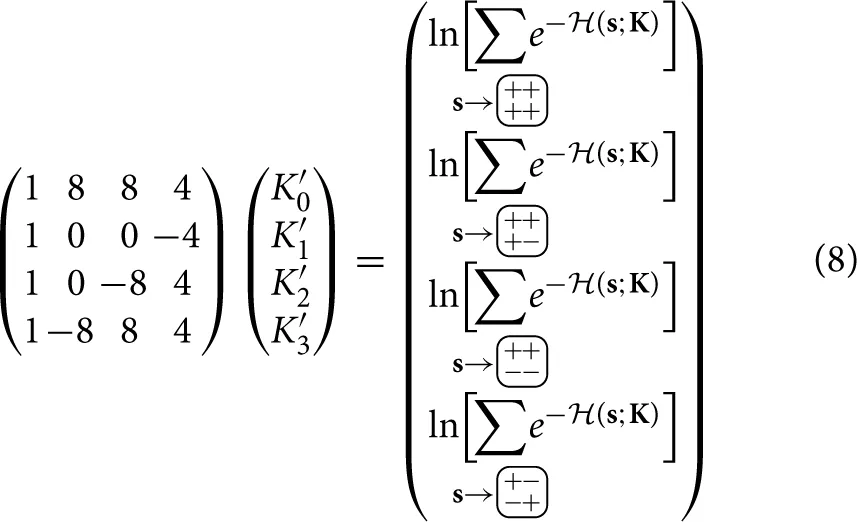
where each of the sums on the right runs over the suitable set of original spin configuration, using the notation

$\begin{array}{cc}{\displaystyle \sum _{s\to S}{\text{e}}^{-{\mathscr{H}}(s;K)}}={\displaystyle \sum _{s\in {\{-1,1\}}^N}T}(S;s){\text{e}}^{-{\mathscr{H}}(s;K)}.& (9)\end{array}$

As discussed above, in principle, there is of course one such equation for each coarse-grained S, but as far as determining K′ from K is concerned, this leads to lines (in Equation 8) being repeated as often as there are configurations in an equivalence class.

Solving the linear system Equation (8) establishes the map

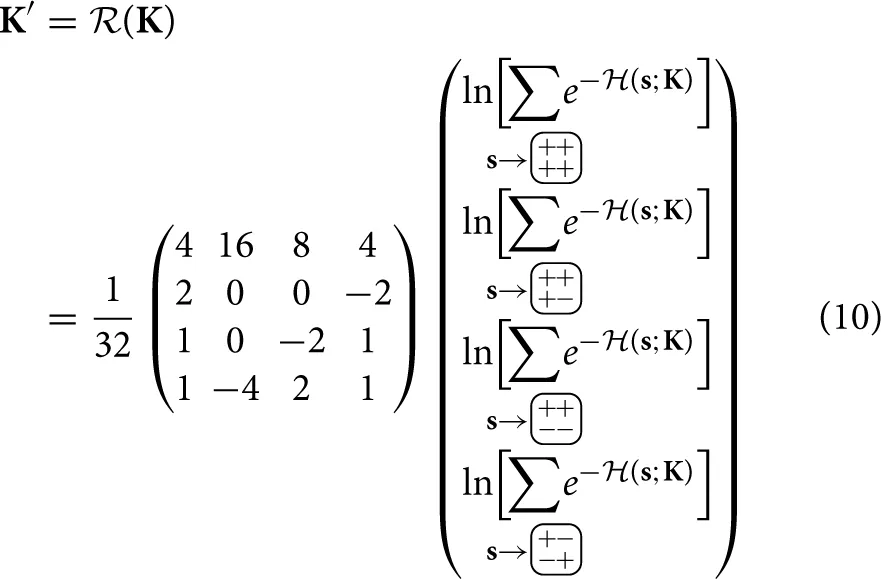
The summation (Equation 9) has to be carried out very many times when hunting for the fixed point K* = ${ℛ}$(K*), using, for example, Newton-Raphson [13]. The Jacobian matrix J_ij = ∂ ${ℛ}$(K)_i/∂ K_j can very easily be determined simultaneously with ${ℛ}$(K) itself, see Section 4.1. It is that sum (Equation 9), that is computationally expensive, even when applying computational tricks (Section 4.1), of varying sophistication. The most obvious one is to run over all possible original configurations s and determine the coarse-grained S for which T(S; s) = 1, rather than fixing S and finding all roots of T(S; s) = 1. By symmetry of the block spin transformation, in a q state Potts Model (q = 2 for Ising) each of the q^N′ has q^N−N′ valid original configurations.

Finding and characterizing a fixed point in a 4 × 4 → 2 × 2 RSRG procedure for the Ising Model is, on a modern laptop computer, a matter of seconds. Extending the procedure to other lattices of the same size has barely an effect on the CPU time, but changes to the dimension of the available phase space volume obviously do.

It turns out that ${ℛ}$(K) as defined in Equation (10) has no fixed point. The reason is that K₀ enters identically on the left and on the right, because it simply gives rise to a factor exp(K₀) in front of the partition sum. Equation (10) can therefore be written as

$\begin{array}{cc}{K}^{\prime }=ℛ(K)=\left(\begin{array}{c}{K}_0+R_0(K_1,K_2,K_3)\\ R_1(K_1,K_2,K_3)\\ R_2(K_1,K_2,K_3)\\ R_3(K_1,K_2,K_3)\end{array}\right),& (11)\end{array}$

and imposing ${ℛ}$(K*) = K* generally has no solution in K*₀ at all, as K*₀ = K*₀ + R₀(K₁, K₂, K₃) poses only an extra condition on K₁, K₂, K₃, which is not generally fulfilled. This is an anomaly that can be resolved by multiplying the offset K₀ by the number of degrees of freedom, as it arises naturally in Section 3, so that N′ K*₀ = NK*₀ + R₀(K₁, K₂, K₃) which has a unique solution K*₀. At this stage, we accept that R₀(K₁, K₂, K₃) represents the additional phase space volume of an 4 × 4 lattice compared to a 2 × 2 lattice. Ignoring its particular value for the time being, we carry on by modifying the renormalization transformation slightly,

$\begin{array}{cc}{\tilde{K}}^{\prime }={\left(\begin{array}{c}{K}_{1^{\prime }},K_{2^{\prime }},K_{3^{\prime }}\end{array}\right)}^T=\widetilde{ℛ}(\tilde{K})=\left(\begin{array}{c}{R}_1(K_1,K_2,K_3)\\ R_2(K_1,K_2,K_3)\\ R_3(K_1,K_2,K_3)\end{array}\right),& (12)\end{array}$

with $\tilde{K}$ = (K₁, K₂, K₃)^T. In other words, the fixed point is determined only in the K₁, K₂, K₃ subspace.

The conventional wisdom of the statistical mechanics of phase transitions has it that there should be three fixed points: One is associated with a divergent correlation length, which is the non-trivial fixed point that we would like to characterize. Two more fixed points exist that have a vanishing correlation length associated with them, the low-temperature fixed point and the high-temperature fixed point. As for the former, it is not a fixed point in the strict sense of $\widetilde{{ℛ}}$($\tilde{K}$*) = $\tilde{K}$* as $\tilde{K}$ diverges under the map $\widetilde{{ℛ}}$($\tilde{K}$).

As for the high-temperature fixed point, one can easily see that K₁ = K₂ = K₃ = 0 is invariant under application of ${ℛ}$(K), Equation (10), as in this case the Boltzmann-factor is simply exp(K₀ in each of the terms on the right, which gives K′₁ = K′₂ = K′₃ = 0 and K′₀ = K₀ + ln(2^N−N′), where 2^N−N′ is the number of terms in the sums.

Once the non-trivial fixed point, $\tilde{K}$* = $\widetilde{{ℛ}}$($\tilde{K}$*), is found, critical exponents can be extracted from a linear stability analysis. These exponents characterize the scale invariance in the neighborhood of the fixed point. As discussed extensively in the textbooks [11], they are related to those eigenvalues λ_x of the Jacobian J = ∂ (K′₀, K′₁, …,)/∂ (K₀, K₁, …) that are greater than 1, corresponding to relevant directions in coupling space. In the following we will refer to them as y_x with

$\begin{array}{cc}{y}_x=\frac{\ln ({\lambda }_x)}{\ln (b)}.& (13)\end{array}$

We use the naming convention x = t (the thermal exponent) for a Hamiltonian that contains no coupling which spoils its invariance under global permutations of the spin state. For example, in the Ising Model, Equation (7) represents such a Hamiltonian, which is invariant under s → −s, as ${\mathscr{H}}$(s; K) = ${\mathscr{H}}$(−s; K). In principle, after introducing one or more external fields there is ambiguity as to which eigenvalue corresponds to which exponent, which can be resolved by studying the Hamiltonian first without these external fields.

Using the procedure described above gives a single positive exponent y_t = 0.936, which is a stunningly good estimate compared to the exact value of y_t = 1/ν = 1 [8, 9]. All exponents calculated in the present work are collected in Table 2, with three significant digits quoted throughout this work.

TABLE 2

Table 2. Critical inverse temperatures and exponents for the Ising Model and q-state Potts Models on the square lattice (for the triangular lattice see Table 8), as determined in the present work (“this work”) or in the literature (“lit.” and references).

2.1. Adding a Magnetic Field

In order to determine the other, well known critical exponent, y_h, we need to allow for a non-vanishing field H in Equation (1),

$\begin{array}{cc}{\mathscr{H}}(s)=-J{\displaystyle \sum _{\langle ij\rangle }{s}_i}{s}_j-H{\displaystyle \sum _i{s}_i}.& (14)\end{array}$

Any H ≠ 0 breaks the parity symmetry of the Hamiltonian, i.e., ${\mathscr{H}}$(s) ≠ ${\mathscr{H}}$(−s). This causes another “level splitting” among the equivalence classes introduced in Table 1, in particular C₀ and C₁, which results in the six classes listed in Table 3. Consequently, we introduce two more couplings in Equation (7), resulting in

$\begin{array}{cc}\begin{array}{l}{\mathscr{H}}(s;K)=-K_0-K_1{\displaystyle \sum _{\langle ij\rangle }{s}_i}{s}_j-K_2{\displaystyle \sum _{\langle \langle ij\rangle \rangle }{s}_i}{s}_j\\ -K_3{\displaystyle \sum _{\langle ijkl\rangle }{s}_i}{s}_j{s}_k{s}_l-K_4{\displaystyle \sum _i{s}_i}-K_5{\displaystyle \sum _{\langle ijk\rangle }{s}_i}{s}_j{s}_k,\end{array}& (15)\end{array}$

where 〈ijk〉 denotes corner-triplets of sites (in any orientation) as shown in Figure 4.

TABLE 3

Table 3. The six equivalence classes of spin configurations (local motives) on a 2 × 2 Ising torus, based on Equation (15).

Performing again a fixed point analysis results in one new exponent y_h = 1.823 (see Table 2) and the same y_t as above. In fact, the values of the couplings K₁, K₂, K₃ at the fixed point do not change at all, while K*₄ = 0 and K*₅ = 0 are new relevant couplings. The analytical value of y_h = 1.875 [14] testifies to the accuracy of the present scheme.

3. Generalization to Categories

The procedure above can be generalized by noticing that in order for Equation (8) to give rise to a fixed point equation, the precise structure of the matrix on the left hand side is irrelevant, as the same linear combination of couplings enters in the Hamiltonian on the right. Reassigning couplings $\tilde{K}$_i according to

$\begin{array}{cc}\tilde{K}=\left(\begin{array}{c}{\tilde{K}}_0\\ {\tilde{K}}_1\\ {\tilde{K}}_2\\ {\tilde{K}}_3\end{array}\right)=M\left(\begin{array}{c}{K}_0\\ K_1\\ K_2\\ K_3\end{array}\right)\text{with}M=\left(\begin{array}{cccc}1& 8& 8& 4\\ 1& 0& 0& -4\\ 1& 0& -8& 4\\ 1& -8& 8& 4\end{array}\right)& (16)\end{array}$

then produces the map $\tilde{K}$′ = M ${ℛ}$(M⁻¹ $\tilde{K}$), which effectively (apart from a factor M) has the same “fixed point” $\tilde{K}$* = MK as the original map ${ℛ}$(K) and, up to linear transform, the same Jacobian, $\frac{{\tilde{K}}^{\prime }}{\tilde{K}}=M\frac{K^{\prime }}{K}{M}^{-1}$. As long as M is invertible, every linear combination of couplings is allowed, with no immediate benefit as far as the properties of the fixed point are concerned, but suggesting a greatly increased range of choices of couplings for different classes of local motives (spin configurations), such as those shown in Table 1 or those in Table 3.

Above, we did not arrive at an actual fixed point equation, $\tilde{K}$* = ${ℛ}$($\tilde{K}$*), because the implied K*₀ = K*₀ + R₀(K*₁, K*₂, K*₃) has generally no solution at all or infinitely many for R₀(K*₁, K*₂, K*₃) = 0. To this end we adjust the new Hamiltonian such that this relation turns into the more desirable form N′$\tilde{K}$′₀ = N$\tilde{K}$₀ + R₀($\tilde{K}$₁, $\tilde{K}$₂, $\tilde{K}$₃), which possesses unique solutions for any given set of couplings $\tilde{K}$₁, $\tilde{K}$₂, $\tilde{K}$₃.

The new Hamiltonian, in the following referred to as the “categories Hamiltonian” reads

$\begin{array}{cc}{\mathscr{H}}(s;K)=-{\displaystyle \sum _{j=0}^{k-1}{K}_j}{\displaystyle \sum _i^N{\delta }_{{𝒞}(s,i),j}}& (17)\end{array}$

where ${𝒞}$(s, i) ∈ {0, 1, …, k − 1} in the Kronecker δ-functions δ_${𝒞}$(s, i), j determines for the configuration s the equivalence class or category of a the local b × b motif rooted at spin i according to the given table of equivalence classes or categories, say Table 1, and a convention regarding orientation like Figure 5. The ∑_j runs over all k categories and ${\Sigma }_i^N$ over all N lattices sites. Equation (17) applies equivalently to coarse-grained configurations where s is replaced by S and N and N′. Correspondingly, the renormalization map based on Equation (17) is

$\begin{array}{cc}{K}^{\prime }=ℛ(K)=\frac{1}{N^{\prime }}\left(\begin{array}{c}\ln \left[{\displaystyle {\sum }_{s\to S_0}{e}^{-{\mathscr{H}}(s;K)}}\right]\\ \ln \left[{\displaystyle {\sum }_{s\to S_1}{e}^{-{\mathscr{H}}(s;K)}}\right]\\ \ln \left[{\displaystyle {\sum }_{s\to S_2}{e}^{-{\mathscr{H}}(s;K)}}\right]\\ ⋮\\ \ln \left[{\displaystyle {\sum }_{s\to S_{k-1}}{e}^{-{\mathscr{H}}(s;K)}}\right]\end{array}\right),& (18)\end{array}$

with S_i in category C_i, in short $K_i^{\prime }=N^{\prime -1}\ln [{\displaystyle {\sum }_{s\to S_i}{e}^{-{\mathscr{H}}(s;K)}}]$. Extrapolating from the discussion about K*₀ above, one coupling to be determined through K* = ${ℛ}$(K*) in Equation (18) should be related to the others by some trivial relationship. In fact, by construction, every fixed point K* of ${ℛ}$(K*) has the property ${ℛ}$(K* + δ𝟙) = K* + b^d δ𝟙 for arbitrary δ and 𝟙 = (1, 1, …, 1)^T, i.e., shifting all couplings by the same amount. This is because Equation (17) gives ${\mathscr{H}}$(s; K + δ𝟙) = −Nδ + ${\mathscr{H}}$(s; K) since ∑_j δ_${𝒞}$(s, i), j = 1 and ${\displaystyle {\sum }_i^N=N=b^d{N}^{\prime }}$.

As far as exponents are concerned, since more generally

$\begin{array}{cc}{K}^{\prime }(K+\delta 𝟙)=ℛ(K+\delta 𝟙)=b^d\delta 𝟙+ℛ(K)=b^d\delta 𝟙+K^{\prime }(K)& (19)\end{array}$

for any K, the Jacobian in the linear stability analysis remains unchanged as $\frac{\partial {K^{\prime }}_i(K+\delta 𝟙)}{\partial K_j}=\frac{\partial {K^{\prime }}_i(K)}{\partial K_j}$, in particular at the fixed point K = K*, resulting in identical estimates for the exponents. In other words, finding a $\tilde{K}$* which is shifted equally in all components after renormalization, ${ℛ}$($\tilde{K}$*)−$\tilde{K}$* = (b^d−1)δ𝟙 is as good as finding a fixed point. The particular choice of δ = −K*₀ makes category 0 disappear from the Hamiltonian at the fixed point, i.e., there is $\tilde{K}$* = (0, K*₁ − K*₀, K*₂ − K*₀, …) such that ${ℛ}$($\tilde{K}$*) = $\tilde{K}$* + (b^d−1) δ𝟙. Since category 0 disappears from the Hamiltonian, one less root has to be found numerically, and indeed δ and thus K*₀ are determined from the shift of $\tilde{K}$* under ${ℛ}$($\tilde{K}$*).

It turns out to be numerically most convenient to use the parameterization

$\begin{array}{cc}\begin{array}{l}{\mathscr{H}}(s;\widehat{K})=-{\widehat{K}}_0{\displaystyle \sum _i{\delta }_{{𝒞}(s,i),0}}-({\widehat{K}}_0+{\widehat{K}}_1){\displaystyle \sum _i{\delta }_{{𝒞}(s,i),1}}\\ -({\widehat{K}}_0+{\widehat{K}}_2){\displaystyle \sum _i{\delta }_{{𝒞}(s,i),2}}-({\widehat{K}}_0+{\widehat{K}}_3){\displaystyle \sum _i{\delta }_{{𝒞}(s,i),3}}\\ =-N{\widehat{K}}_0-{\displaystyle \sum _{j=1}^{k-1}{\widehat{K}}_j}{\displaystyle \sum _i^N{\delta }_{{𝒞}(s,i),j}}\end{array}& (20)\end{array}$

which corresponds to Hamiltonian Equation (17) with K = ($\widehat{K}$₀, $\widehat{K}$₀ + $\widehat{K}$₁, $\widehat{K}$₀ + $\widehat{K}$₂, …) and so the transform of $\widehat{K}$ trivially derives from that of K according to Equation (18), so that ${\widehat{K}}^{\prime }$($\widehat{K}$) = A⁻¹ ${ℛ}$(A$\widehat{K}$) with

$A=\left(\begin{array}{c}1000\dots \\ 1100\dots \\ 1010\dots \\ \dots \end{array}\right).$

The proper fixed point $\widehat{K}$* = A⁻¹${ℛ}$(A$\widehat{\text{K}}$*) = A⁻¹ K* needs to be determined only up to arbitrary $\widehat{\text{K}}$₀, as Equation (19) implies

$\begin{array}{cc}{\widehat{K}}^{\prime }(\widehat{K}+\delta {(1,0,0,\dots )}^T)={\widehat{K}}^{\prime }(\widehat{K})+b^d\delta {(1,0,0,\dots )}^T& (21)\end{array}$

and the estimates of the exponents are unaffected by the specific value of $\widehat{\text{K}}$₀, as discussed above. From Equation (21) it follows that the first column of the Jacobian is

$\begin{array}{cc}\frac{\partial {\widehat{K}}^{\prime }}{\partial K_0}={(b^d,0,0,\dots )}^T,& (22)\end{array}$

which leads to an eigenvector of the form (1, 0, 0, …)^T and an eigenvalue of λ = b^d and thus an exponent y₀ = d, Equation (13). Correspondingly, 𝟙 is an eigenvector of the Jacobian of K′(K) with eigenvalue b^d, see Equation (19).

Formulating the Hamiltonian in terms of categories frees us from the need to come up with enough (complicated) n-point interactions (as we did in Equation 7) to match the number of equivalence classes (such as Table 1). Rather, each equivalence class is assigned a particular coupling, so their numbers match by definition.

The new form of the Hamiltonian Equations (17) or (20) allows for more radical changes, as there is no need to construct the classes of local motives in reference to the original Hamiltonian, such as Equation (1). In this light, the previous choice of four categories (equivalence classes) for the real-space renormalization of Equation (1), as listed in Table 1, was somewhat arbitrary. The particular feature of this partitioning of the N′ configurations is that all configurations within a category are related by symmetry operations induced by the properties of the underlying lattice or, in the absence of external fields, by spin reversal. Configurations from different classes cannot be related by any such operation.

However, the original Hamiltonian Equation (1) has only three different energy levels, as configurations in categories C₁ and C₂ have the same energy. It appears justified to enforce that this property is preserved under renormalization, i.e., to demand that there are only three categories, namely C₀, C₁ ∪ C₂ and C₃.

A subtlety arises when merging categories such that the resulting set contains configurations, which are not related by the lattice or spin symmetries (see the discussion after Equation 6), because now coarse-grained configurations S₁ and S₂ may have the same energy, ${\mathscr{H}}$′(S₁; K′) = ${\mathscr{H}}$′(S₂; K′) without, however, being related by lattice symmetry operations that could equally be applied to the set of s₁ with T(S₁; s₁) = 1. To accommodate this change, we modify Equation (6),

$\begin{array}{cc}{\displaystyle \sum _{S\in C}{\text{e}}^{-{{\mathscr{H}}}^{\prime }(S;K^{\prime })}}={\displaystyle \sum _{S\in C}{\displaystyle \sum _{s\in {\{-1,1\}}^N}T}}(S;s){\text{e}}^{-{\mathscr{H}}(s;K)}& (23)\end{array}$

where the sum ∑_S∈C runs over all coarse-grained configurations S in C. With ∑_i∑_S∈Ci = ∑_S this restores Z′(K′) = Z(K).

By definition exp (−${\mathscr{H}}$′(S₁; K′)) = exp (−${\mathscr{H}}$′(S₂; K′)) for any pair S₁, S₂ ∈ C, so the left hand side in Equation (23) is |C| exp(−${\mathscr{H}}$′(S; K′)), with |C| the cardinality of the category C ∋ S. A similar simplification can be applied on the right, as

$\begin{array}{cc}{\displaystyle \sum _{s\in {\{-1,1\}}^N}T}(S_1;s){\text{e}}^{-{\mathscr{H}}(s;K)}={\displaystyle \sum _{s\in {\{-1,1\}}^N}T}(S_2;s){\text{e}}^{-{\mathscr{H}}(s;K)}& (24)\end{array}$

for any two S₁, S₂ that are related by lattice symmetry operations. Above, these equivalence classes were referred to as “classes,” the (possible) union of which we generalized to categories. To compute the right hand side in Equation (23) only one representative or paradigm is needed for each equivalence class. If C is the union of the (former) classes C₁ and C₂ with paradigms S₁ and S₂ respectively, then Equation (23) can be re-written as

$\begin{array}{cc}\begin{array}{l}{\text{e}}^{-{{\mathscr{H}}}^{\prime }(S_1;K^{\prime })}={\text{e}}^{-{{\mathscr{H}}}^{\prime }(S_2;K^{\prime })}\\ =\frac{\left|C_1\right|}{\left|C\right|}{\displaystyle \sum _{s\in {\{-1,1\}}^N}T}(S_1;s){\text{e}}^{-{\mathscr{H}}(s;K)}\\ +\frac{\left|C_2\right|}{\left|C\right|}{\displaystyle \sum _{s\in {\{-1,1\}}^N}T}(S_1;s){\text{e}}^{-{\mathscr{H}}(s;K)}.\end{array}& (25)\end{array}$

With the set-up mentioned above (three categories, C₀, C₁ ∪ C₂, and C₃ as of Table 1) the exponents found are y₀ = 2 (trivially) and y_t = 0.929 (see Table 2).

The possibility to create categories as unions of equivalence classes reduces the number of couplings and thus the dimensionality of the space to consider in search for a fixed point. There is, in principle, no reason to keep certain configurations together in the same category, even when that may break the symmetries of the lattice. The six categories shown in Table 3 are, in that sense, minimal, in that each category contains exactly one representative and (all) its translations (on a periodically closed lattice), so that any two configurations are related by lattice symmetries. For the sake of computability, we may, however, strive to reduce the number of categories and break them up only if induced by the application of an external field. Table 1 is minimal in the sense that each category contains all configurations equivalent not only under translation but in addition also under spin reversal, the latter a symmetry broken by an external magnetic field. In principle, all symmetries could be broken, such that there are N′ categories, corresponding to a maximum number of external fields. It turns out, however, that only very few of these fields produce an exponent and that many choices result in a singular matrix M, Equation (16).

Exploring the possibility of merging amongst the four original equivalence classes in Table 1, two can be merged (in $\left(\begin{array}{c}4\\ 2\end{array}\right)$ = 6 ways), resulting in three classes, three can be merged (in four ways) leaving only one class intact, or two pairs can be merged each (in three ways). Merging all four trivially produces only one exponent, y₀ = 2. Of the thirteen non-trivial parameterizations, only parameterizations which leave the ground state configurations and in a class of their own result in a fixed point being found, see Table 4.

TABLE 4

Table 4. All thirteen non-trivial unions of categories based on the original four categories listed in Table 1.

Most of these choices combine categories with different energies according to the original Ising Hamiltonian and consequently the critical temperature can no longer be calculated. How that is done is discussed in the following.

3.1. Estimating the Critical Temperature

The critical temperature T_c is originally defined on the basis of the Hamiltonian Equation (1) and the partition sum Equation (2), as the value of T in the effective coupling J/(k_BT) at the critical point. At the critical point, the couplings in the partition sum approach under renormalization the non-trivial fixed point determined above. In fact, an entire subspace of the coupling space, namely the basin of attraction, flows toward that fixed point. The critical point is thus the intersection of the basin of attraction and the “physical line.” The physical line is determined by the linear map between the coupling J/(k_BT) of the original Hamiltonian, e.g., Equation (1), and the couplings K, see Equation (7), such that

$\begin{array}{cc}\frac{1}{k_{B}T}{{\mathscr{H}}}_{\text{Ising}}(s)={{\mathscr{H}}}_0+{\mathscr{H}}(s;K),& (26)\end{array}$

with some additive constant ${\mathscr{H}}$₀, independent of the individual configurations s, which represents a possible overall energy offset that has no impact on any physical observable. For fixed J and k_B, Equation (26) provides a map K(T), linear in J/(k_BT).

Equation (26) holds for all s simultaneously and therefore is, in principle, a set of 2^N (independent) equations, which means that K(T) is hugely overdetermined. Even taking into account the various different symmetries leaves a vast number of equations, much larger than the set Equations (6) or (23). In the case of the set of couplings used in Equation (7), however, this Hamiltonian is in fact identical to Equation (1) for K₀ = K₂ = K₃ = 0 and K₁ = J/(k_BT). Even after moving to the more convenient set of couplings $\tilde{K}$ via Equation (16), the identity remains unchanged except for the trivial, linear map outlined in Equation (16).

Finding the couplings of a categories Hamiltonian such that it matches an original, physically motivated Hamiltonian is straight-forward as long as the former forms a superset of the interactions contained in the latter. For example, using the categories of Table 1 with C₁ and C₂ merged, so that C₀ has coupling $\tilde{K}$₀, C₁ ∪ C₂ coupling $\tilde{K}$₁₂ and C₃ coupling $\tilde{K}$₃, the set of linearly independent equations to determine the couplings in Equation (20) is given by

$\begin{array}{cc}4{\tilde{K}}_0+{{\mathscr{H}}}_0=8\frac{J}{k_{B}T}& (27\text{a})\end{array}$

$\begin{array}{cc}4{\tilde{K}}_0+4{\tilde{K}}_{12}+{{\mathscr{H}}}_0=0& (27\text{b})\end{array}$

$\begin{array}{cc}4{\tilde{K}}_0+4{\tilde{K}}_3+{{\mathscr{H}}}_0=-8\frac{J}{k_{B}T}& (27\text{c})\end{array}$

where the factor 4 on the left accounts for the effect of summing over all 2 × 2 neighborhoods, see Figure 5. Technically, the first and third equations are repeated twice and the second twelve times. In the present parameterization, the arbitrary offset ${\mathscr{H}}$₀ may be absorbed into $\tilde{K}$₀. The temperature T thus determines effectively only $\tilde{K}$₃.

Obviously, such a mapping Equation (27) is possible only for those categories Hamiltonians, that do not merge configurations that have different energies in the original Hamiltonian, as otherwise the same left hand side is equated to different right hand sides.

Once the map $\tilde{K}$(T) is established, the critical temperature T_c, is found as the $\tilde{K}$(T_c) which ultimately flows into the fixed point, i.e., repeated application of the renormalization scheme ${ℛ}$ such as Equations (10) or (18) drives $\tilde{K}$(T_c) to the fixed point $\tilde{K}$* = ${ℛ}$($\tilde{K}$*),

$\begin{array}{cc}ℛ(ℛ(\dots ℛ(\tilde{K}(T_c))\dots ))={\tilde{K}}^{\ast }.& (28)\end{array}$

In order to find T_c the linearization about the fixed point is of little use, as the renormalization flow becomes non-linear away from it. Numerically, the most efficient way of finding the critical temperature is thus a divide-and-conquer scheme, whereby a reasonable interval of (inverse) temperatures is split into regions according to the fixed point that is approached under successive application of ${ℛ}$. Above T_c, i.e., T > T_c, all $\tilde{K}$(T) flow toward the high-temperature fixed point $\tilde{K}$(T → ∞) → 0. Below T_c, i.e., T < T_c, some or all of the components of $\tilde{K}$(T) diverge (see Figure 7). The critical temperature T_c is to be found between those regions, bracketed by successively picking a temperature between one that is known to flow toward the high-temperature fixed point and one that flows toward the low-temperature fixed point.

FIGURE 7

Figure 7. The flow induced by repeated application of the map ${ℛ}$(K) from different starting points in the K₁–K₂ plane, see Equation (7). A separatrix between flow toward the high- and low-temperature fixed points is clearly visible. This is the basin of attraction of the fixed point. Its intersection with the line K₂ = 0 (and K₃ = 0) determines K_1c = ${\left(\frac{J}{k_{B}T}\right)}_c$.

The second column in Table 2 lists the temperatures that we found for the different models considered. In general, inverse temperatures are mildly underestimated, which may be explained by the small lattices suppressing some fluctuations.

3.2. Potts Model

In the following, we present the analysis of the Potts Model. The approach using categories avoids the use of n-point interactions to provide enough couplings for the set of equivalence classes in the Potts Model, which otherwise would prove rather messy [15].

The procedures outlined above can obviously quite easily be extended to the q-state Potts Model [7, Equation (1.6)] which (traditionally) has Hamiltonian

$\begin{array}{cc}{\mathscr{H}}(s)=-J{\displaystyle \sum _{\langle ij\rangle }{\delta }_{s_i,s_j}}-H{\displaystyle \sum _i{\delta }_{s_i,0}}& (29)\end{array}$

where s_i ∈ {0, 1, …, q − 1} and the Kronecker δ-function favors equality of nearest neighbors for positive J and s_i = 0 for H > 0. For q = 2 the Ising Hamiltonian Equation (1) is recovered up to a constant shift of the energy and a factor 2 in the couplings, which has no impact on the value of the exponents. For q = 3 and in the absence of an external field, the minimal set of categories is shown in Table 6. The thermal exponent found is y_t = 1.118 compared to y_t = 1.2 analytically [16], again in very good agreement (see Table 2).

The situation becomes significantly more complicated when an external field is applied, such as H in Equation (29), which breaks the permutation symmetry S₃ down to S₂, as the Hamiltonian remains invariant under permutations of the two states 1 and 2 which do not couple to H. Without using unions of equivalence classes as categories, the number of couplings needed for the q = 3 Potts Model in an external field is 13, shown in Table 5. Again, this set of categories is minimal, in the sense that each category contains only those configurations which are related to each other by lattice translations and (global) permutations of state 1 and 2. The resulting magnetic exponent is y_h1 = 1.810 (Table 2), again in very good agreement with the theoretical value of y_h1 = 1.866… [17].

TABLE 5

Table 5. The six equivalence classes of the 3-state Potts Model (with states 0, 1, and 2 as shown) on a 2 × 2 lattice.

The presence of a single external field promoting one particular state in a q > 2-state Potts Model is peculiar, as the phase space selected by favoring one state, say 0 via positive external field H, is fundamentally different from the phase space selected by −H, which favors q − 1 states that have an S_q−1 symmetry between them. A linearization about the fixed point, as used in the derivation of the exponents, is blind to such a (non-linear) change of character, i.e., each eigenvector of the Jacobian is associated with only one exponent. The number of categories (and couplings) however, arising from the application of a single field allows for many more new relevant directions.

In fact, the exponent y_h1 may be thought of as characterising the continuous phase transition at the endpoint of a line of first order transitions between a phase with a majority of 0 states and a mixed phase of state 1 and 2. A second line of first order transitions exist between phases where a single state has a majority, say, between 0 and 1. The introduction of a single field does in fact produce a second magnetic exponent y_h2, whose numerical value y_h2 = 0.614 (also listed in Table 2) should be compared to the values reported in the literature of y_h2 = 0.55 [16] and y_h2 = $\frac{2}{3}$ [18]. In the present picture, it seems that the external field has a projection on the relevant direction associated with this second magnetic exponent. It may thus also be interpreted as a subleading term (associated with a confluent singularity) visible in a perturbation by an external field such as the one in Equation (29).

Dividing the categories up further by introducing a second external field, thereby breaking symmetry (the remaining S₂) down one last time, causes further splitting of the categories listed in Table 6 (to 21 categories) and produces a second pair of exponents y_h1 and y_h2 which are numerically identical to the ones produced above, so in total 6 relevant (positive) exponents are observed, namely y₀ = 2 and y_t, as well as y_h1 and y_h2 each twice. That second breaking of symmetry has exhausted all remaining symmetries and no further external fields can be introduced. If the second is thought of as mediating a transition between phases with majority states 1 and 2 respectively, then suitable linear combinations between the first and the second external field will mediate transitions between any majority or mixed states.

TABLE 6

Table 6. The 13 equivalence classes of the 3-state Potts Model (with states 0, 1, and 2 as shown) on a 2 × 2 lattice in the presence of an external field coupling to state 0.

We took a similar approach for the q = 4 Potts Model. The resulting exponents were y_t = 1.296 and y_h1 = 1.814 (Table 2) compared to y_t = 1.5 [19] and y_h1 = 1.875 [16] in the literature. The “second magnetic exponent” y_h2 = 0.682 (compared to the theoretical value y_h2 = 0.875 [16]) is again visible with only one external field. However, a third magnetic exponent y_h3 = 0.174 (as well as a second pair of y_h1 and y_h2) appears when introducing a second field. We are not aware of this exponent being discussed in the literature. It may be associated with a transition between, say, a mixed phase with mostly states 0 and 2 and one with mostly 1 and 3, i.e., favoring pairs of states. Table 7 lists the number of categories and which exponents appear under the application of external fields. It is well-known that there exists a marginal exponent or logarithmic correction to y_t because q = 4 is the marginal value of q above which the transition becomes first order in d = 2 dimensions [20]. However, despite the relatively small value of y_h3 (0.174 on the square lattice, Table 2, and 0.099 on the triangular lattice, Table 8), this exponent should not be mistaken as a correction, as its appearance follows the same pattern as the other magnetic exponents, on the square lattice as well as on the triangular lattice, see Table 7. In contrast, the exponent y_t, which is not related to the application of external magnetic fields, occurs only once, regardless of how many external fields are applied.

TABLE 7

Table 7. Introducing more symmetry breaking external fields produces an increasing number of (minimal) categories and exponents.

TABLE 8

Table 8. Critical inverse temperatures and exponents for the Ising Model and q-state Potts Models on the triangular lattice (for the square lattice see Table 2), as determined in the present work (“this work”) or in the literature (“lit.” and references).

Introducing a dedicated field which couples equally to 0 and 2 spins has the effect of leaving a symmetry in place between 0 and 2 spins as well as between 1 and 3 spins. This field splits for example the category containing the four configurations 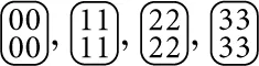in two, namely in one containing and and another one containing and . A less obvious result of breaking symmetry in such a way is that the category which contains all four different spin states (which exists for only if q ≥ 4) will also split. This is because and are related by swapping 0 and 2 and/or swapping 1 and 3, whereas and are not related by this symmetry operation. This demonstrates the need to differentiate between the notion of an external field coupling to a certain spin species as it does in the Ising or Potts Hamiltonian, and an external field breaking a (permutation) symmetry. Introducing such a field results in 22 categories. All three magnetic exponents, as well as the thermal and trivial exponent are observed exactly once (i.e., there are no repeated exponents). The values are exactly those found when introducing two external fields. The existence of y_h3 in the presence of such a field and its absence without such a field reinforces our interpretation that this exponent is not related to logarithmic corrections to scaling with temperature.

3.3. Other Fixed Points

The BEG Model or spin-1 Ising Model, introduced by Blume, Emery and Griffiths to describe the behavior of a ³He − ⁴He mixture [21], has the Hamiltonian (without external field)

$\begin{array}{cc}H=-J{\displaystyle \sum _{\langle ij\rangle }{s}_i}{s}_j-K{\displaystyle \sum _{\langle ij\rangle }{s}_i^2}{s}_j^2+\Delta {\displaystyle \sum _i{s}_i^2}& (30)\end{array}$

with s_i ∈ {−1, 0, 1}. This Hamiltonian is invariant under the global parity transformation s_i → −s_i, i.e., the inversion of all spins. Unlike the 3-state Potts Model, however, it is not invariant under other permutations of the three states {−1, 0, 1}. This is reminiscent of the 3-state Potts Model in an external field coupling to state 0, which is equivalent to offsetting the Hamiltonian by a constant and a coupling equally to states 1 and 2. This is similar to the effect of the products s_i s_j and (s_i s_j)² in Equation (30), which singles state s_i = 0 out. In fact, the 13 categories of the Potts Model, Table 6, also form the minimal set of categories of the BEG Model, if state 2 is mapped to spin orientation s_i = −1.

The magnetic (and thermal exponents) of the 3-state Potts Model with a single external field as discussed above were determined using the couplings at the fixed point of the transform for the model without external field, as discussed in Section 2.1. This fixed point is unique in the sense that its basin of attraction intersects with the physical line of the Potts Model Equation (29). To find a fixed point that is associated with the BEG Model, one has to widen the net and consider the entire 13 dimensional coupling space. It is, of course, futile to scour this space systematically without the constraint of a physical line or any other special locus.

We therefore resorted to random, uniform sampling over a reasonable range of couplings, rejecting the known Potts and the trivial fixed points. Computationally, it takes under a minute to determine the fixed point a particular parameter set flows to. Two further fixed points were revealed by the process, which we discuss in the following. Both fixed points have the usual structure of a fixed point with external field, i.e., the Jacobian has three eigenvalues greater than unity, namely y₀ = 2 as well as two further, non-trivial exponents y_{1, 2}.

The couplings at the first alternative fixed point are such that a symmetry of states 1 and 2 in the Potts Model (1 and −1 of the BEG Model) is implemented, that is to say, configurations have the same energy under local changes of state 1 to state 2 and vice versa. For example, 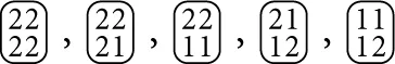and all have the same energy at the fixed point, and similarly 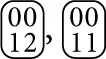, and have the same energy as well. Considering categories with the same energy for a moment as identical, the resulting set of categories is that of the Ising Model in an external field, associating states 1 and 2 with, say, up spins (+) and 0 with down spins (−) and interpreting the “entropic advantage” of the former as the effect of an external field. The critical exponents of y₁ = 0.927 and y₂ = 1.837 appear to support this rather artificial interpretation. However, the symmetries at the fixed point sit well with the BEG Model which for J = 0 in Equation (30) is invariant under local parity transforms s_i → −s_i, while providing more phase space for |s_i| = 1 compared to s_i = 0.

The second alternative fixed point has a lower symmetry, as no local permutation are allowed, that is to say, at the fixed point no two couplings are equal. Furthermore, the numerical value of the couplings at the fixed point are unusually large, imposing a heavy energetic penalty on configurations containing 1 − 2 nearest neighbour pairs. The critical exponents found are y₁ = 0.700 and y₂ = 1.722. We can only speculate that this fixed point may also be related to the rich phase diagram of the BEG model, known to have a variety of transitions [22].

It seems reasonable to expect that the exponents of higher spin Ising Model can be found as fixed points of higher q-state Potts Models. For example, the categories of the spin $\frac{3}{2}$ Ising Model with s_i ∈ {−3, −1, 1, 3} are identical to those of the 4-state Potts Model in the presence of a single field which couples identically to two of the four states.

3.3.1. Reconstructing the Ising Fixed Point

The conventional wisdom of statistical physics [7] would argue that one can always introduce p strong external fields in a q-state Potts Model to suppress the occurrence of p states, resulting in a q − p-state Potts Model. For example, applying a strong magnetic field in the 3-state Potts Model should reveal the Ising fixed point. This will be the Ising fixed point without external field as the only external field present is the one that suppresses one species without coupling (differently) to the remaining two species.

In our scheme, this fixed point should feature as a further alternative fixed point in the 3-state Potts Model with a single external field, however with unusually large or even divergent (negative) couplings in the presence of the disfavored species. Having recourse to Table 6, we set the couplings related to configurations C₁, C₃, C₄, C₆, C₈, C₉, C₁₀, C₁₁, and C₁₂ such that these configurations are penalized and the couplings related to configurations C₀, C₂, C₅, and C₇ are set to the fixed point values of the corresponding four we found for the Ising Model (compare Table 1 and Table 6). While the large (penalizing) coupling renormalize to larger values, we find the couplings related to the (allowable) categories C₀, C₂, C₅, and C₇ to stay fixed under the renormalization scheme, as expected. Correspondingly, we find the same y_t as produced by the scheme based on Table 1.

3.4. 6 × 6 Lattices

At least for q = 2, it is numerically feasible to study larger lattices, such as N = 6. While a stronger rescaling of b = 3 is possible, b = 2 is more promising as it results in a larger coarse-grained lattice of 3 × 3. It turns out that N = 6, b = 2 is also less memory intensive, because there are fewer original configurations per coarse-grained one, namely 2^(N2)/2^(N2/b2). This is partially compensated by the N/b × N/b patches falling into 13 categories for b = 2 and into 4 for b = 3, namely the same as for N = 4, b = 2, see Table 1. Consequently, N = 6, b = 3 is approximately three times as memory intensive as N = 6, b = 2, rendering the former feasible with the computational resources available to us but not the latter. The scheme finds two exponents as expected, namely y₀ = 2, and the thermal critical exponent y_t = 0.980. This is a significant improvement compared to y_t = 0.936 in Table 2.

3.5. Triangular Lattice

Implementing the scheme developed above on a triangular lattice is considerably more complicated as rhombic patches have to be constructed in multiple orientations which respect the boundary conditions. Likewise, taking the boundary conditions into account when generating the categories is more difficult for triangular than square lattices. The motivation of doing so is to validate the scheme and to demonstrate that the remarkable accuracy of the estimated critical exponents is not dependent on using a square lattice, but, in fact, inherent to the scheme.

Table 8 summarizes our findings on the triangular lattice. In general, the inverse critical temperatures are more strongly underestimated compared to our findings for the square lattice Table 2. On the other hand, the thermal exponents, y_t, are generally found to be closer to the theoretical values, whereas the first magnetic exponents y_h seem systematically underestimated. Because different theoretical estimates for the q = 3 second magnetic exponent y_h2 exist [16, 18], our estimates are not easily validated, but the results in Table 8 and Table 2 differ by only 6% or less. The existence of the third magnetic exponent y_h3 is confirmed, but its estimate of 0.099 is significantly smaller than on the square lattice (0.174). Although the numerical value may thus be questioned, we strongly believe that it exists in the thermodynamic limit. Finally, the pattern of repeated magnetic exponents as summarized in Table 7 is recovered on the triangular lattice.

Furthermore, in the case of the Ising Model in the presence of a single magnetic field, it seemed reasonable that the categories obtained by our method should likewise be capable of capturing the physics of the Baxter-Wu model [23]. This would manifest itself in there being a second, non-trivial fixed point which we however were unable to locate using a wide range of initial conditions for the couplings in our Newton-Raphson scheme. A considerably wider range of random starting points can be probed for the Ising Model compared to the 3 state Potts Model, as the process of converging to a fixed point from a given starting configuration typically takes a fraction of a second.

3.6. q = 5 Potts Model

The critical point of the q-state Potts Model in two dimensions ceases to exist when q is increased beyond q = 4 [7, 24]. Subject to a lengthy historical discussion, the transition in temperature T (or, equivalently, J in Equation 29) becomes first order for q = 5 (in 2 dimensions) and beyond. We were hoping to see this reflected in the apparent absence of a non-trivial fixed point, or at least absence of a fixed point whose basin of attraction intersects the physical line, Section 3.1.

The absence of a critical point for q ≥ 5 has been associated with the presence of effective vacancies (or voids) [25], where none of a spin's neighbors is in the same state as that spin, i.e., all δ_{si, sj} for a give spin i vanish in Equation (29). On the square lattice, such local configurations exist for q ≥ 2 and can extend across macroscopic parts of the lattice. However, with increasing q they are highly degenerate and thus acquire a large weight in the partition sum.

It has been long known that conventional renormalization group methods fail to capture this effect [15]. For example, using the majority rule and dilatation by a factor b = 2, as we have above, replaces by a single spin and thus may dramatically overestimate its contribution to long range order.

Nienhuis et al. managed to recover the first order transition for q = 5 and above by replacing such “disordered” patches by effective holes [25]. We have explored a different route, motivated by the work by Berker and Andelman [26], who, using Monte Carlo, could demonstrate that a slightly modified Potts Hamiltonian (cf. Equation 29) produces continuous phase transitions for q as high as 20. Their modification amounted to energetically penalizing effective vacancies by raising the energy of 2 × 2 patches of the form . In the original Hamiltonian, Equation (29), such patches have the same energy as those of the form or . In a minimal set of categories, and all of its permutation (in the absence of an external field) are contained in the same category and can thus be energetically penalized or favored, depending on the coupling. One may therefore speculate that the (undesirable) fixed point found by our scheme was the one encountered by Berker and Andelman, i.e., one where effective vacancies are suppressed.

To avoid this unintended suppression, we merged categories according to the original Hamiltonian Equation (29), as discussed in Section 3 for the Ising Model. For q = 3, 4, 5 this results in only 4, 5, and 5 categories respectively. The resulting estimates for the exponents differ only marginally from those obtained by using the full minimal set of categories, and a non-trivial fixed point for the 5-state Potts Model was indeed found again (see Table 9).

TABLE 9

Table 9. The inverse critical temperatures and exponents y_t as obtained by grouping categories based on the original Potts Model Hamiltonian (this work, see text) in comparison to literature values (lit.).

Another strategy is to revise the disambiguation of the majority rule, which crudely replaces, say

by the fully ordered . This can be done by allowing the indicator function T(S; s), Equation (5), to carry a weight, so that, for example,

contributes with a weight of 1/4 to and , as if the patch coarse grains to 0, 1, 2 and 3 each with a weight of 1/4. As a result, highly disordered (and thus ambiguous) configurations contribute comparatively little to any given sum ∑_{s → S}, but likewise contribute to several sums simultaneously. Performing this process does not only consume much more CPU-time (compared to top left rule), but requires significantly more memory, see Table 10. Applying the process to q = 4, for which estimates of y_t are somewhat less accurate than for q = 2 and q = 3, does, however, not result in improved exponent estimates. Given the computing resources available, we were unable to apply this technique to q = 5.

TABLE 10

Table 10. Memory requirements for g^a→b_j in the q = 2,3,4,5-state Potts Model with N = 4, b = 2 and in the absence of a magnetic field.

In conclusion, it would appear that our method cannot easily be adjusted to allow us to observe the change of transition from continuous to first order when q is increased from q = 4 to q = 5. One may hope that this can be achieved by reconciling our categories Hamiltonian method with Nienhuis et al.'s special treatment of effective vacancies when performing the coarse-graining.

4. Discussion

In the present section we first review a number of implementation details and “numerical tricks” some of which yield a considerable speed-up. In the second part, we summarize the findings above.

4.1. Numerical Techniques

The CPU-time spent on the renormalization procedure is essentially determined by the time it takes to calculate the sums on the right of the transformations Equations (10) or (18) and the number of times the transform itself is invoked. In the following, we list some measures to improve the computational performance.

(1) As outlined above, of the q^N′ renormalized configurations of size L′ × L′ in a q-state Potts Model many are related by the lattice symmetries leading to the classes and categories such as those listed in Table 1 or Table 3. To reduce the CPU-time, only those configurations that renormalize to a small number of representatives (paradigms) need to be generated. This may be achieved by using a dictionary that divides the q^b2 states of the b × b patches into q coarse-grained configurations. This dictionary is consulted for the purpose-built generation of all original configurations that renormalize to a given paradigm.

Alternatively, one may start out considering all q^N configurations and determine whether and, if so, which paradigm they renormalize to. This was done by generating a table to map each of the q^b2 configurations to a one of q possible values. The renormalization of b × b patches inside the L × L configuration can be sped up by stopping as soon as it is found that the resulting coarse grained configuration cannot possibly belong to any of the paradigms. For example, if the left-most coarse-grained configurations in Table 1 are the paradigms, which all have a + spin in the top left corner, then having a − spin in the top left corner means that the configuration cannot possibly result in a paradigm.

(2) In principle, the Jacobian J_ij = ∂ ${ℛ}$(K)_i/∂ K_j can be determined numerically. However, the derivatives according, say Equation (18), are easily computed along with the Boltzmann-factor itself, such as

$\begin{array}{cc}\frac{\partial \widetilde{{ℛ}}{(K)}_i}{\partial K_j}=\frac{{\displaystyle {\sum }_{s\to C_i}\left({\displaystyle {\sum }_k^N{\delta }_{{𝒞}(s,k),j}}\right)}{e}^{-{\mathscr{H}}(s;\tilde{K})}}{{\displaystyle {\sum }_{s\to C_i}{e}^{-{\mathscr{H}}(s;\tilde{K})}}}& \left(31\right)\end{array}$

for Equation (17) and similarly for the more complicated Hamiltonians discussed above, such as Equation (7). Calculating the Jacobian in this form improves both numerical accuracy of the Jacobian and speed of the computation.

(3) When calculating the Boltzmann-factor, exp(−${\mathscr{H}}$), frequent calls of the library function exp(double) can be avoided by using a lookup-table which stores the exponential of each coupling. In modern architectures, fast numerical co-processors compared to relatively slow memory access might question the benefit of this measure. We found that there was no noticeable speed-up using such a dictionary.

(4) However, the use of a more extensive lookup table g^a→b_j described in the following made a considerable difference. It stores all information to determine the energy of an L × L configuration indexed by a, which coarse-grains to a particular L′ × L′ configuration b. No reference is otherwise retained to determine the specific original configuration a. If T(S; s) (defined in Equation 5) is either 0 or 1, then by symmetry, the q^N original configurations divide into q^N′ coarse-grained configurations, i.e., a ∈ {1, 2, …, q^{N − N′}}. The table g^a→b_j gives the coefficients in front of all couplings K_j with j = 0, 1, …, k − 1 in the Hamiltonian, so that

$\begin{array}{cc}{\mathscr{H}}(s_a;K)={\displaystyle \sum _{j=0}^{k-1}{g}_j^{a\to b}}{K}_j& (32)\end{array}$

where s_a coarse grains to S_b. The sum Equation (6) can thus be written

$\begin{array}{cc}{\displaystyle \sum _{s\in {\{-1,1\}}^N}T}(S_b;s){\text{e}}^{-{\mathscr{H}}(s;K)}={\displaystyle \sum _{a=1}^{q^{N-N^{\prime }}}{\text{e}}^{-{\displaystyle {\sum }_j{g}_j^{a\to b}{K}_j}}}.& (33)\end{array}$

The table g^a→b_j has to determined only for those coarse-grained configurations b which are paradigms, of which there are k, the number of categories. Because g^a→b_j stores the k coefficients in front of the couplings K_j for each original configuration, memory requirements scale in total like k²q^{N − N′}, i.e., memory needs to be allocated for k²q^{N − N′} entries. The values stored in g^a→b_j range from 0 to at most n, namely the number of spins (and thus patches) in the original configuration. As N = 16 < 255 in our case, a single byte for each entry suffices for our purposes. If T(S; s) is allowed to have values different from 0 and 1, then effectively more original configurations a contribute to the coarse-grained configuration b, namely q^N−N′ original configuration plus ambiguous ones. In addition, the weight T(S_b; s_a) has to be stored. The memory requirements for q = 2, 3, 4, 5 are listed in Table 10.

Once determined, g^a→b_j effectively relieves us from determining the energy of the original (non-coarse-grained) configurations over and over, namely each time ${ℛ}$(K) is invoked.

The speed-up is considerable. For example, on a reasonably modern laptop computer, generating g^a→b_j for a q = 4 Potts Model on a square lattice takes about 7 min, reducing the time to calculate ${ℛ}$(K) to about 30 s, a reduction by a factor 15 compared to the CPU-time spent on the same task without g^a→b_j. The table g^a→b_j can also be used to calculate derivatives as it contains the information necessary to evaluate Equation (31).

4.2. Discussion and Summary

In the present work we have attempted to improve and generalize a particularly simple realspace renormalization scheme as first suggested by Hasenbusch [4]. The aim was to understand realspace renormalization and its limitations and to extend the scheme to characterize the q = 3, 4, 5 Potts Models and their magnetic exponents. The present scheme can be used on different lattices and for a comparatively large number of local states, as we investigated systems with up to about 152 · 10⁹ states.

Although the lattices we have used are minimalistic and, in fact, ridiculously small compared to what is used in modern Monte-Carlo simulations [27], the resulting exponents and estimates of the critical temperature are surprisingly good, typically within 3–7% on the square lattice and within 5 – 20% on the triangular lattice. We were able to systematically investigate the Potts Model with q = 2 to q = 5 states and determine a whole range of magnetic exponents, some of which are disputed (y_h2 [16, 18]) or have not previously been reported in the literature (y_h3).

Given the high quality of the results and the consistency, we had hoped to find the first order transition of the q = 5 Potts Model reproduced in our approach. Unfortunately, we found a fixed point even in effective Hamiltonians, which treat certain local motifs, so-called “effective vacancies,” more efficiently. The q = 5 Potts Model, however, is known to have defied numerics in the past [15].

One may wonder whether the present approach can be used successfully in higher dimensions, say the Ising Model in three dimensions, which, however, has about 18 · 10¹⁸ states. Considering our computationally fastest method, the amount of configurations which must be generated is approximately 1.21 · 10¹² larger than for the q = 5 Potts Model, which takes approximately one day to run on current computer equipment. The memory requirements on the other hand would be 6.71 · 10⁷ k² GiB, with k the number of categories. Without performing the analysis explicitly, we estimate the number of categories would turn out to be roughly ten meaning the current method would require roughly 6.7 EiB of RAM and is thus clearly out of the reach with current resources available.

Conflict of Interest Statement

The authors declare that the research was conducted in the absence of any commercial or financial relationships that could be construed as a potential conflict of interest.

References

1. Wilson KG. Renormalization group and critical phenomena. I. Renormalization group and the kadanoff scaling picture. Phys Rev B (1971) 4:3174–83. doi: 10.1103/PhysRevB.4.3174

CrossRef Full Text | Google Scholar

2. Wilson KG. Problems in physics with many scales of length. Sci Am. (1979) 241:140–57. doi: 10.1038/scientificamerican0879-158

CrossRef Full Text | Google Scholar

3. Kadanoff LP. Scaling laws for Ising models near T*_c. Physics (1966) 2:263–72.

Google Scholar

4. Hasenbusch M. Finite Lattice RG-Transformation for the 2d Ising Model, Lectures Notes. Humboldt-Universität zu Berlin (1999).

5. Ising E. Beitrag zur theorie des ferromagnetismus. Z Phys. (1925) 31:253–8. doi: 10.1007/BF02980577

CrossRef Full Text | Google Scholar

6. Potts RB. Some generalized order-disorder transformations. Math Proc Camb. (1952) 48:106–9. doi: 10.1017/S0305004100027419

CrossRef Full Text | Google Scholar

7. Wu FY. The potts model. Rev Mod Phys. (1982) 54:235–68. doi: 10.1103/RevModPhys.54.235

CrossRef Full Text | Google Scholar

8. Stanley HE. Introduction to Phase Transitions and Critical Phenomena. New York, NY: Oxford University Press (1971).

Google Scholar

9. Efrati E, Wang Z, Kolan A, Kadanoff LP. Real-space renormalization in statistical mechanics. Rev Mod Phys. (2014) 86:647–67. doi: 10.1103/RevModPhys.86.647

Pubmed Abstract | Pubmed Full Text | CrossRef Full Text | Google Scholar

10. Le Bellac M. Quantum and Statistical Field Theory [Phenomenes Critiques Aux Champs de Jauge, English]. New York, NY: Oxford University Press (1991).

Google Scholar

11. Cardy J. Scaling and Renormalization in Statistical Physics. Cambridge, UK: Cambridge University Press (1997).

Google Scholar

12. Binney JJ, Dowrick NJ, Fisher AJ, Newman MEJ. The Theory of Critical Phenomena. Oxford, UK: Oxford University Press (1998).

Google Scholar

13. Press WH, Teukolsky SA, Vetterling WT, Flannery BP. Numerical Recipes, 3rd Edn. Cambridge, UK: Cambridge University Press (2007).

Google Scholar

14. Onsager L. Crystal statistics. I. A two-dimensional odel with an order-disorder transition. Phys Rev. (1944) 65:117–49. doi: 10.1103/PhysRev.65.117

CrossRef Full Text | Google Scholar

15. Dasgupta C. Renormalization-group study of the Ashkin-Teller-Potts model in two dimensions. Phys Rev B (1977) 15:3460–4. doi: 10.1103/PhysRevB.15.3460

CrossRef Full Text | Google Scholar

16. Nienhuis B, Riedel EK, Schick M. Magnetic exponents of the two-dimensional q-state Potts model. J Phys A Math Gen. (1980) 13:L189–92. doi: 10.1088/0305-4470/13/6/005

CrossRef Full Text | Google Scholar

17. Blöte HWJ, Nightingale MP, Derrida B., Critical exponents of two-dimensional Potts and bond percolation models. J Phys A Math Gen. (1981) 14:L45. doi: 10.1088/0305-4470/14/2/005

Pubmed Abstract | Pubmed Full Text | CrossRef Full Text | Google Scholar

18. Swendsen RH, Berker AN. Critical behavior of the three-state Potts model: monte carlo renormalization group. Phys Rev B (1983) 28:3897–903. doi: 10.1103/PhysRevB.28.3897

Pubmed Abstract | Pubmed Full Text | CrossRef Full Text | Google Scholar

19. den Nijs MPM. A relation between the temperature exponents of the eight-vertex and q-state Potts model. J Phys A Math Gen. (1979) 12:1857. doi: 10.1088/0305-4470/12/10/030

CrossRef Full Text | Google Scholar

20. Swendsen RH, Andelman D, Berker AN. Critical exponents and marginality of the four-state Potts model: monte carlo renormalization group. Phys Rev B (1981) 24:6732–5. doi: 10.1103/PhysRevB.24.6732

CrossRef Full Text | Google Scholar

21. Blume M, Emery VJ, Griffiths RB. Ising model for the λ transition and phase separation in He³ − He⁴ mixtures. Phys Rev A (1971) 4:1071–7. doi: 10.1103/PhysRevA.4.1071

CrossRef Full Text | Google Scholar

22. Berker AN, Wortis M. Blume-emery-griffiths-potts model in two dimensions: phase diagram and critical properties from a position-space renormalization group. Phys Rev B (1976) 14:4946–63. doi: 10.1103/PhysRevB.14.4946

CrossRef Full Text | Google Scholar

23. Baxter RJ, Wu FY. Exact solution of an Ising model with three-Spin interactions on a triangular lattice. Phys Rev Lett. (1973) 31:1294–7. doi: 10.1103/PhysRevLett.31.1294

Pubmed Abstract | Pubmed Full Text | CrossRef Full Text | Google Scholar

24. Baxter RJ. Potts model at the critical temperature. J Phys C Solid State Phys. (1973) 6:L445–8. doi: 10.1088/0022-3719/6/23/005

CrossRef Full Text | Google Scholar

25. Nienhuis B, Berker AN, Riedel EK, Schick M. First- and second-order phase transitions in Potts models: renormalization-group solution. Phys Rev Lett. (1979) 43:737–40. doi: 10.1103/PhysRevLett.43.737

CrossRef Full Text | Google Scholar

26. Berker AN, Andelman D. First- and second-order phase transitions in Potts models: competing mechanisms (invited). J Appl Phys. (1982) 53:7923–26. doi: 10.1063/1.330231

CrossRef Full Text | Google Scholar

27. Moloney NR, Pruessner G. Asynchronously parallelized percolation on distributed machines. Phys Rev E. (2003) 67:037701. doi: 10.1103/PhysRevE.67.037701

Pubmed Abstract | Pubmed Full Text | CrossRef Full Text | Google Scholar

28. Fisher ME. The theory of equilibrium critical phenomena. Rep Prog Phys. (1967) 30:671. doi: 10.1088/0034-4885/30/2/306

CrossRef Full Text | Google Scholar