Estimating the ground-state probability of a quantum simulation with product-state measurements

1. Introduction

The Hilbert space that describes a strongly correlated many-body quantum system grows exponentially in the number of particles N, so determining the ground state of a complex many-body quantum system becomes numerically intractable when the size of the quantum system becomes too large to be represented on a classical computer (unless there is some other simplification, like weak entanglement, etc.). Feynman introduced the idea to simulate complex many-body quantum systems on a quantum computer in the 1980's [1]. Since Feynman's proposal, quantum algorithms have been developed to calculate eigenvalues and eigenvectors of these intractable systems [2]. One of the challenges with creating the ground state on a quantum computer, say by adiabatic evolution of the ground state from a simple to a complex one, is how do we determine the extent of the ground-state preparation. After all, we do not know what the ground state is a priori so it is difficult to know what the final probability to be in the ground state is. In this work, we propose one method to estimate the probability to remain in the ground state. While this analysis is applied to ion-trap emulators (that model interacting spin systems), the general discussion can be applied to any quantum computer that performs ground state preparation, but creates diabatic excitations as a result of a too rapid time evolution. To date, trapped-ion quantum simulators have seen success in two different platforms: the Penning trap has trapped ≈300 ions in a planar geometry and generated Ising spin interactions [3] and the linear Paul trap has performed quantum simulations with up to 18 ions in a one-dimensional crystal [4]. Other types of quantum simulation, like digital Trotter evolution [5], have also been tried, but that form of computation does not benefit from the analysis we present here. The success of these traps as quantum simulators is attributed to their long coherence times, precise spin control, and high fidelity. Here, we focus on the linear Paul trap quantum simulator.

In an ion trap quantum simulator, hyperfine states of the trapped ions are used for the different spin states (for simplicity, we can consider only two states, and hence, a spin-one-half system). Optical pumping can be employed to create a product state with the ions all in one of the two hyperfine states with fidelities close to 100%. A coherent rotation of that state can then be used to create any global rotation of that product state. By turning on a large magnetic field, this state can be configured to be the ground state of the system. Then the magnetic field is reduced slowly enough for the system to remain in the ground state until the system evolves into the complex spin Hamiltonian in zero magnetic field. The challenge is that the evolution of the system must be completed within the coherence time of the spins, which often is too short to be able to maintain adiabaticity throughout the evolution (and indeed, becomes increasingly difficult as the system size gets larger). In order to estimate the probability to remain in the ground state during the time-evolution of the simulation, we envision testing the probability that the system is in the ground state at a specific time, called t_stop (where the Hamiltonian becomes independent of time), by first evolving the system from the initial time to t_stop, and then measuring the expectation value of an observable as a function of time for later times. The oscillations in the amplitude of the expectation value are given by ${O}(t)=\langle \psi (t)|\widehat{{O}}|\psi (t)\rangle$ (with |ψ(t)〉 the quantum state of the system at time t > t_stop). The time evolution of the observable, ${O}$(t), oscillates at frequencies given by the energy differences between the final eigenstates (where the Hamiltonian becomes time independent). More concretely, let $\widehat{{H}}(t_{stop})|m\rangle =E_m|m\rangle$, then the time-dependent expectation value satisfies

$\begin{array}{cc}{O}(t>t_{stop})={\displaystyle \sum _{mn}{P}_m^{\ast }}{P}_n\langle m|\widehat{{O}}|n\rangle \exp [-i(E_n-E_m)t],& (1)\end{array}$

where P_m = 〈m|ψ(t_stop)〉 is the overlap of the state |ψ(t_stop)〉 with the eigenstate |m〉 (we have set ℏ = 1). Since we will be measuring the probability to be in a product state, the operator $\widehat{{O}}$, is a projection operator onto the particular product state, denoted |ϕ〉, or $\widehat{{O}}=|\varphi \rangle \langle \varphi |$. Previously, we showed how Fourier transforming the time series and employing signal processing methods like compressive sensing, allows one to extract the energy differences as a type of many-body eigenstate spectroscopy [6, 7]. Here, we focus on the amplitude of the oscillations, given by $P_1^{*}{P}_n\langle 1|\widehat{{O}}|n\rangle$, which is proportional to the probability amplitude of the ground state (P₁). Note that we do not need to know the explicit ground-state wavefunction to estimate its probability from these oscillations. This is the main advantage of this technique. One might ask what happens to this approach if the ground state (or an excited state) is degenerate? Since we have the freedom to express the eigenbasis within each degenerate manifold, we choose the first state within the manifold to be the state that |ψ(t_stop)〉 projects onto. Then the overlap with all other states within each degenerate manifold is zero, and the system reverts to the non-degenerate problem. This approach may become complicated if the projection onto the degenerate subspace changes as a function of t_stop, but since the probability to be within a degenerate subspace should be a continuous function of time, this should not cause any further issues, as it just redefines the basis within the subspaces as a function of t_stop. However, a priori the energy difference between the ground state and the first excited state is not known and these two states can be nearly degenerate. If the energy difference becomes too small such that during the measurement (t > t_stop) the state does not appear to change with time, then we will not see the oscillation and will conclude the system remained in the ground state. This poses as a limitation of our analysis, in which either the time interval must be extended to observe the oscillation or a more refined analysis must be applied (such as compressive sensing that can determine the Fourier spectra without observing the compete oscillation [8]).

We first illustrate how the the ground-state probability can be estimated by analyzing the amplitude of the oscillations of the simplest time-dependent Hamiltonian: the two-level Landau-Zener problem. The Landau-Zener problem is defined via

$\begin{array}{cc}\widehat{{H}}(t)={\sigma }^x-B^z(t){\sigma }^z.& (2)\end{array}$

Here σ^α are the Pauli spin operators in the α = x, y, or z direction. The Pauli spin operators have the commutation relation

$\begin{array}{cc}\left[{\sigma }^{\alpha },{\sigma }^{\beta }\right]=2i{ϵ}_{\alpha \beta \gamma }{\sigma }^{\gamma },& (3)\end{array}$

where the Greek letters represent the spatial directions and ϵ_αβγ is the antisymmetric tensor. The Landau-Zener problem has a minimum energy gap occurring when B^z(t) = 0, as shown in Figure 1. Since the Landau-Zener problem is a two state system, the probabilities, P₁ and P₂, are related by $P_2^2=1-P_1^2$ and the state, |ψ(t)〉, can be represented by P₁ = cos(ϕ) and P₂ = sin(ϕ). Using this state in Equation (1), we find that the expectation value ${O}$(t > t_stop) becomes (neglecting terms with no time dependence)

$\begin{array}{cc}\begin{array}{l}{O}(t>t_{stop})=\cos (\varphi )\sin (\varphi )\{\langle 1|\widehat{{O}}|2\rangle \exp [-i(E_2-E_1)t]\hfill \\ +\langle 2|\widehat{{O}}|1\rangle \exp [-i(E_1-E_2)t]\}.\hfill \end{array}\hfill & (4)\hfill \end{array}$

FIGURE 1

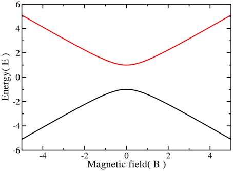
Figure 1. The energy spectra of the Landau-Zener problem. There is a minimum energy gap when the excited state, in red, lies at its minimum energy difference with the ground state. This occurs at B^z(t) = 0.

The ground-state probability [cos²(ϕ)] can then be calculated if $\langle 1|\widehat{{O}}|2\rangle$ is known. The amplitude of the oscillations is $sin(2\varphi )\langle 1|\widehat{{O}}|2\rangle$. Although the matrix element $\langle 1|\widehat{{O}}|2\rangle$ can be directly measured when the amplitude reaches a maximum, at ϕ = π∕4, because the matrix element depends on the magnetic field at t_stop, it changes with different $B^z(t_{stop})$, so determining the matrix element for all fields is complicated. In addition, even if ϕ is extracted from the amplitude, there are always two solutions, except when ϕ = π∕4 (see Figure 2), and hence two possible ground state probabilities. In Figure 2, we show both the amplitude of the oscillations and the ground-state probability as a function of ϕ, where the dashed line shows that the amplitude is not unique to a single ground-state probability. However, for systems with many quantum states, one does not have a simple closed set of equations and the analysis of the amplitude of the oscillations can only estimate the ground-state probability when the ground-state amplitude is dominant in |ψ(t)〉. We demonstrate this below with the transverse field Ising model.

FIGURE 2

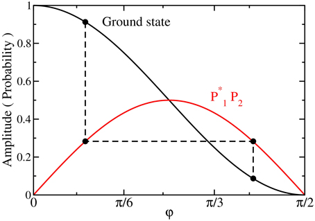
Figure 2. Analytic solutions to the Landau-Zener problem showing the ground-state probability (black solid line) and the reduced amplitude of the oscillations, $P_1^{*}{P}_2$, of ${O}$(t > t_stop) (red solid line). The reduced amplitude of the oscillations is not unique to a single ground-state probability, as highlighted by the dashed line. The full oscillation amplitude is $P_1^{*}{P}_2\langle 1|\widehat{{O}}|2\rangle$ and requires knowledge of the matrix element as well.

It is well known that the amount of diabatic excitation in the Landau-Zener problem increases the faster the magnetic field is ramped from −∞ to +∞. The general protocol that we employ is as follows (and is depicted schematically in Figure 3):

1. Initialize the state in an arbitrary state. In the following examples, we initialize the state in the ground state of the Hamiltonian with a large polarizing magnetic field.

2. Decrease the magnetic field as a function of time to evolve the quantum state, as shown in Figure 3A, where, for concreteness, we show an example of a magnetic field that changes linearly.

3. Hold the magnetic field at its final value which is first reached at t = t_stop until the measurement is performed at the time interval t_meas. after the field has been held constant (see Figure 3A).

4. Measure an observable of interest, ${O}$(t), for a number of different t_meas. values.

5. Determine the amplitude of the oscillations.

FIGURE 3

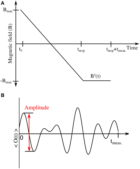
Figure 3. Schematic diagram of the experimental protocol. (A) The transverse magnetic field as a function of time is diabatically ramped down to a chosen value, $B^z(t_{stop})$. $B^z(t_{stop})$ is then held for a time interval of t_meas.. (B) An observable is measured at the end of the interval t_meas.. The amplitude of the oscillation is taken, for simplicity, to be the amplitude of the initial oscillation after t_stop.

Note that one requirement of this approach is that the observable of interest must oscillate as a function in time as given in Equation (1). The amplitude is extracted from the first maximum and minimum of the observable as a function of time by

$\begin{array}{cc}Amplitude=\frac{\text{max}[{O}(t)]-\text{min}[{O}(t)]}{2}& (5)\end{array}$

The time evolution of the wavefunction |ψ(t)〉 is calculated by solving the time-dependent Schrödinger equation:

$\begin{array}{cc}i\frac{\partial }{\partial t}|\psi (t)\rangle =\widehat{{H}}(t)|\psi (t)\rangle & (6)\end{array}$

by using the Crank-Nicolson method to time evolve the state |ψ(t)〉. This technique solves the problem with the following approach [9]

$\begin{array}{cc}\left(\widehat{𝕀}+i\frac{\delta t}{2}\widehat{{H}}(t+\delta t)\right)|\psi (t+\delta t)\rangle =\left(\widehat{𝕀}-i\frac{\delta t}{2}\widehat{{H}}(t)\right)|\psi (t)\rangle .& (7)\end{array}$

Note that the Hamiltonian is time-dependent until t_stop is reached, when it becomes constant in time and thereafter the solution is trivial to obtain.

We present a numerical example to illustrate this protocol by analyzing the oscillations for the Landau-Zener problem. Due to the fact that the eigenstates for the Landau-Zener problem at $|B^z(t_{stop})|\gg 1$ approach the eigenstates of the σ^z operator, if one measures an operator that is diagonal in this basis, there will be no oscillations in the expectation value because the matrix element coupling the two states together vanishes. Hence, we measure the expectation value of the operator $\widehat{{O}}(\theta )$, the Pauli spin matrix that points in the θ direction.

$\begin{array}{cc}\widehat{{O}}(\theta )=R^{†}(\theta ){\sigma }^{z}R(\theta ),& (8)\end{array}$

where R(θ) is the global rotation about the y-axis and is given by

$\begin{array}{cc}R(\theta )=\widehat{𝕀}\cos \left(\frac{\theta }{2}\right)+i{\sigma }^y\sin \left(\frac{\theta }{2}\right),\hfill & (9)\hfill \end{array}$

where θ = π∕2 produces $\widehat{{O}}(\theta =\pi ∕2)={\sigma }^x$.

For our numerical examples with the Landau-Zener problem, we use a linear ramp, $B^z(t)=B_0-\tau t$, where B₀ > 0. B₀ is chosen to be large in comparison to 1 to polarize the spin. We evolve the state to t_stop, such that $|B^z(t_{stop}|)\gg 1$. We present the time evolution for 4 different t_stop = 480.0, 221.5, 144.0, and 80.0 for 3 different θ = π∕9, π∕3, and π∕2 in Figure 4. The amplitude of the oscillations becomes 1 when θ = π∕2. When t_stop = 144.0 the amplitude of the oscillations is maximized in comparison to the 3 other t_stop's. Note that because P₁ and P₂ are solely functions of t_stop, the amplitude of the oscillations is maximized by maximizing the overlap matrix element $\langle 1|\widehat{{O}}|2\rangle$, since we do not know how to do this a priori, in an experiment, one simply looks at the amplitude of some parameter and varies the parameter until the amplitude is maximal. We do this to achieve the highest signal with the shortest data collection time. Once again, no knowledge of the ground state is needed to do this, just sufficient variation of the operator with respect to some parameter that results in a large amplitude oscillation.

FIGURE 4

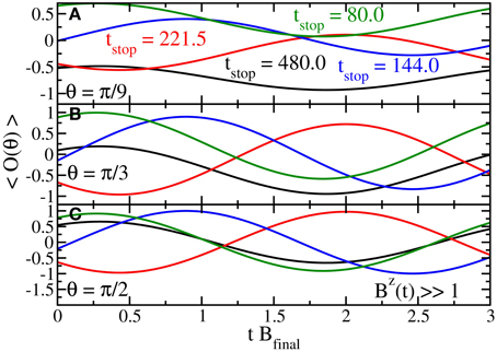
Figure 4. Time evolution of the measurement of $\widehat{{O}}(\theta )$ in the Landau-Zener problem for t_stop = 480.0 (black), 221.5 (red), 144.0 (blue), and 80.0 (green) using θ = π∕6 (A), π∕3 (B), and π∕2 (C). The measurement is being done when B^z(t) ≫ 1. The amplitude of the oscillations converge to 1 as θ is increased to π∕2.

In Figure 5, we show the probability of the ground state compared to the amplitude of the oscillations as a function of t_stop. The amplitude of the oscillations increases as θ is increased. This is due to the σ^x term dominating the $\widehat{{O}}(\theta )$ operator instead of the σ^z term. When the ground-state probability approaches 0.5 the amplitude of the oscillations is maximal and it decreases either when the ground-state probability increases or decreases. As the probability of ground state approaches 1 the amplitude is expected to become 0, which can be obscured due to experimental noise. In order to determine which side of the maximum the measurement of the amplitude is on, experiments with multiple values of t_stop must be run to track the depletion of the ground state as the amplitude of the oscillations reaches a maximum and then decreases. Note further that in this case, since there is only one excited state, one can, in principle, always determine the ground-state probability by measuring the amplitude of the oscillation and extracting the appropriate probability amplitude, if the matrix element $\langle 1|\widehat{{O}}|2\rangle$ is known. For the Landau-Zener problem the eigenstates of the system depend on the magnetic field and the matrix element at that field can be calculated. Alternatively, the $\langle 1|\widehat{{O}}|2\rangle$ can be approximated when the amplitude reaches a maximum, since at this point $|P_1{|}^2\approx 0.5$ and $|P_2{|}^2\approx 0.5$. For more complex systems, such a procedure will not be possible, but the monotonic nature of the curve (at least while the probability for the ground state remains above 50%) will allow us to qualitatively determine whether a given run of the experiment increases the probability to be in the ground state, which can be employed to optimize the ground-state preparation if it is done with some alternative quantum control method besides adiabatically evolving the system. Indeed, we believe this has the potential to be the most important application of this approach. For example, if one wants to try a shortcut to adiabaticity [10], which is known not to be exact, but needs to be optimized as a function of some parameter, then all we want to know is whether the probability to be in the ground state increases or decreases as we change the parameter. The approach described here should work well for this application.

FIGURE 5

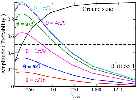
Figure 5. Analysis of the amplitude of the oscillation for the Landau-Zener problem as a function of the t_stop for 6 different θ's. The dashed line is when the ground-state probability is 0.5. As θ increases to π∕2 the amplitude scale increases as well. When the ground-state probability is near 0.5 the amplitude of the oscillations is maximized and the amplitude decreases when either the ground-state probability decreases or increases. Note the strong correlation between the increase of the amplitude of the oscillations and the decrease of the probability to be in the ground state when it is depleted from 100% to about 50%. Beyond this point, it becomes much more difficult to estimate, especially if experimental noise is included in the data.

This simple example shows us a number of important points. First, one may need to rotate the measurement basis if the final product basis are eigenvectors of the Hamiltonian. Second, as the ground state is depleted, the amplitude of the oscillations grows until it reaches a maximum, when the system is equally populating both eigenstates. If the ground state is further depleted, the amplitude of the oscillations will decrease. One can make a mistake in estimating the probability in the ground state if one does not know which side of the curve one is on (probability of the ground state below or above 50%). On the other hand, if one knows which side of the curve one is on, due to making measurements at earlier times to track the ground-state depletion, then one might be able to further use the amplitude to determine the ground state probability in the Landau-Zener problem. When we change to the ion-trap system and examine the transverse-field Ising model, then the procedure becomes more complicated because there are more states that the ground state can be depleted into, and this complicates the analysis. But the method still remains valuable if one can qualitatively determine whether the probability is increasing or decreasing for any set of experiments where we try to optimize the probability to remain within the ground state. Such approaches may become difficult once the ground state is depleted too much. Experimental noise may also complicate the analysis. While the effect of counting statistics is simple to incorporate based on the total number of measurements needed to determine an oscillation amplitude of a particular size, other systematic experimental errors will be specific to the given experiment and difficult to estimate here.

2. Transverse-field Ising Model

Now we describe a more realistic case of the transverse-field Ising model. An ion in the linear chain has two hyperfine states that are separated by a frequency ω_o. The Ising-like interaction is produced by a spin-dependent force that couples the spin to the motional degrees of freedom: this force arises by applying laser light detuned from a Raman transition with two beatnote frequencies of ω_o ± μ—details can be found in Islam et al. [11]. The transverse-field Ising model for N particles is given by

$\begin{array}{cc}\widehat{{H}}(t)=-J_{\pm }{\displaystyle \sum _{i<j}^N{J}_{ij}}{\sigma }_i^z{\sigma }_j^z-B^x(t){\displaystyle \sum _{i=1}^N{\sigma }_i^x},& (10)\end{array}$

where the explicit formula for J_ij is given by Zhu et al. [12]

$\begin{array}{cc}{J}_{ij}={\Omega }^2{\nu }_R{\displaystyle \sum _{\nu =1}^N\frac{b_{i\nu }^{\ast }{b}_{j\nu }}{{\mu }^2-{\omega }_{\nu }^2}}& (11)\end{array}$

and J_± = ±1. Here b_iν is the normalized eigenvector of the νth phonon mode, ω_ν is the corresponding frequency, Ω is the single spin flip Rabi frequency, and ν_R is the recoil frequency associated with the spin-dependent force that depends on the mass of the trapped ion and the difference in wavevector between the laser beams, from which we define our energy units with $J_0={\Omega }^2{\nu }_R$. We work with μ tuned to the blue of the largest ω_ν (which here is the center-of-mass phonon, ω_COM). The Pauli spin matrices are now associated with each lattice site. In this work, we focus on a chain with N = 10 ions. The details of calculating the J_ij and an in depth meaning of the various terms in this equation can be found elsewhere [13]. The spin-spin coupling decays with a power law in the distance, $J_{ij}\propto |r_{ij}{|}^{-\alpha }$ with r_ij the interparticle distance and the exponent α being tunable between 0 and 3. The exponent α is tuned by changing μ or by changing the ratio of the longitudinal to the transverse trap frequencies. Here, we study the ferromagnetic interaction of the Ising model with J_± = 1.

The J_ij of the transverse-field Ising model have a spatial-reflection symmetry such that J_ij = J_N−iN−j and the eigenstates have a parity symmetry with respect to this spatial reflection. The eigenstates of the transverse-field Ising model also have a spin-reflection parity; that is, they have an eigenvalue of ±1 under the partial inversion transformation σ^x → σ^x, σ^y → −σ^y, and σ^z → −σ^z. The spin-reflection parity and spatial-reflection symmetry produce avoided crossings between eigenstates with the same parity and spatial symmetry, such that a minimum energy gap to the lowest coupled state occurs as shown in Figure 6 where we work with parameters for the ion chain with the exponent α ≈ 1. Of course, eigenstates with different symmetries are allowed to cross.

FIGURE 6

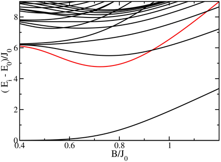
Figure 6. The energy spectra of the ferromagnetic transverse-field Ising model with N = 10. The red curve shows the first coupled excited state and the minimal gap occurs at B^x ≈ 0.72.

The experimental protocol is essentially the same as before. The first difference is that the transverse magnetic field now depends exponentially as a function of time and is given by

$\begin{array}{cc}{B}^x(t)=B_o{\exp }^{-\frac{t}{\tau }},& (12)\end{array}$

as shown in Figure 7A. We choose an exponential decay of the magnetic field, because that is the functional form commonly used in experiments. This choice allows the magnetic field to change rapidly when the gap is large and to have a slower change when the gap is small. But this choice is not the optimal ramp of the magnetic field; it is a compromise between determining a complex shape for the field ramp, and trying to minimize diabatic excitation. The second difference is that we perform two different experimental protocols where the initial state is evolved to t_stop = 6τ and before the time interval t_meas. starts, the magnetic field is quenched to zero $B^x(t_{meas.})=0$, as shown in Figure 7A, or the transverse magnetic field is held at its final value which is first reached at t = t_stop, as depicted in Figure 7B.

FIGURE 7

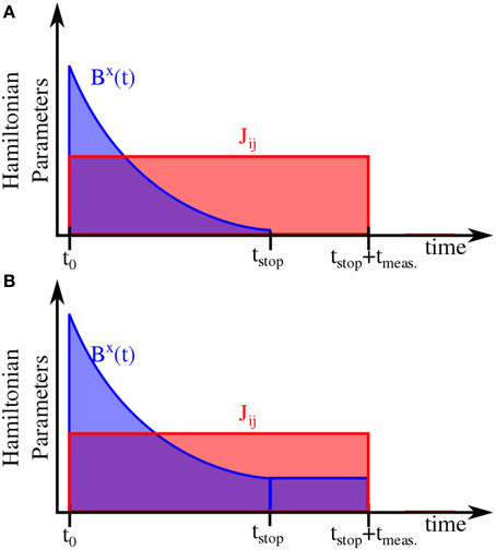
Figure 7. Schematic diagram of the experimental protocol used for the transverse field Ising model. (A) The transverse magnetic field as a function of time is diabatically ramped down to a chosen value, $B^x(t_{stop}=6\tau )$. Then B^x(t) is immediately quenched to 0 before the start of the measurement time interval, t_meas.. (B) The transverse magnetic field is ramped down and held constant at a final value determined by t = t_stop.

There are a number of additional complications. First off, the eigenstates at B^x = 0 are product states along the z direction, hence we need to rotate the measurement basis again to see any oscillations. We choose $\widehat{{O}}(\theta )$ to be the average magnetization in the θ-direction

$\begin{array}{cc}\widehat{{O}}(\theta )=\frac{1}{N}{R}^{†}(\theta ){\displaystyle \sum _{i=1}^N{\sigma }_i^z}R(\theta ),& (13)\end{array}$

where R(θ) is now the global rotation given by

$\begin{array}{cc}R(\theta )={\displaystyle \prod _{i=1}^N\left[\widehat{𝕀}\cos \left(\frac{\theta }{2}\right)+i{\sigma }_i^y\sin \left(\frac{\theta }{2}\right)\right]},\hfill & (14)\hfill \end{array}$

and where θ = π∕2 yields ${\sigma }_{\text{tot}}^x$. Measuring the average magnetization in the θ-direction produces the needed oscillations. There might be other observables that have larger amplitudes, but we choose the average magnetization along an arbitrary axis direction, which is the simplest observable to measure experimentally. At short times, when the excitation out of the ground state is small, the approach proposed here will not work because experimental uncertainty and noise will wash out the ability to measure small amplitude signals. In this regime, if one has enough information about the low-lying spectrum and matrix elements coupling states together, then one can use the adiabatic perturbation theory analysis of Wang and Freericks [14] to approximate the ground-state probability. Of course, those formulas only hold when the excitation is small. Once it becomes large enough, then the methods described here must be employed.

We next show simulated data for the transverse-field Ising model with J_± = 1 and J₀ = 1 kHz. The parameters for the J_ij are μ = 1.0219ω_COM and the antisymmetric ratio of the trap frequencies is 0.691∕4.8 which results in an α ≈ 1.0. The initial state is evolved to t_stop = 6τ and then immediately quenched to zero, as shown in Figure 7A.

In Figure 8, we show the time evolution of ${O}$(θ) with θ = π∕9, π∕3, and π∕2 for 3 different τJ₀ = 0.2, 0.4, and 0.6. The amplitude of the oscillations follow a similar trend to Figure 4, such that at τ = 0.4 the amplitude of the oscillations are at a maximum in comparison to other τ's. Additionally, as θ is increased to π∕2 the amplitude of the oscillations increase as previously seen in the Landau-Zener example.

FIGURE 8

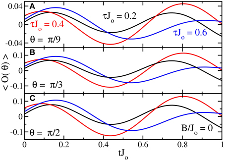
Figure 8. Three different examples of $\widehat{{O}}(\theta )$ as a function of time when τ = 0.2 (black), 0.4 (red), and 0.6 (blue) for θ = π∕6 (A), π∕3 (B), and π∕2 (C) at B∕J_o = 0. t_stop always equals 6τ here.

In Figure 9, we compare the probability of the ground state to the amplitude as a function of the ramping τ. In general, the amplitude of the oscillations is maximized near τ = 0.4 when the ground-state probability is ≈0.61 and the amplitude decreases as the probability to be in the ground state either increases or decreases. Similar to the Landau-Zener problem, as the probability to be in the ground state increases to 1 the amplitude will decrease to 0. However, when the ground-state probability approaches 0.5, the amplitude of the oscillations is now a local minimum (near τJ_o = 0.3). As previously seen in the Landau-Zener example, a single measurement of the amplitude ramped at τ cannot determine whether the probability of the ground state is high or low. Hence, the probability needs to be tracked by using a series of measurements.

FIGURE 9

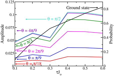
Figure 9. Amplitude of the oscillations at B∕J_o = 0 as a function of different τ as compared to the ground state probability. The arrows for each curve point toward the appropriate vertical axis. As the θ increases, the amplitude of the oscillations increases as well. The amplitude of the oscillations become a maximum when the ground state probability is near 0.6 and the amplitude decreases when the ground state probability increases above or decreases below 0.6. When τ = 0.3 there is a local minimum in the amplitude.

In general, the analysis of the amplitude can be performed for different t_stop's in which the transverse magnetic field is held constant at the strength of $B^x(t_{stop})$, shown in Figure 7B. Figure 10 shows the amplitude of the oscillations as a function of $B^x(t_{stop})$ for 3 different τ = 0.2, 0.4, and 0.6. The amplitude of the oscillations increases as the transverse magnetic field approaches the minimum energy gap and the excitations are created from the ground state, depending on the τ. Once past the minimum energy gap, the ground-state probability increases as de-excitations occur and conversely the amplitude of the oscillations decrease as well. However, a similar response will occur if excitations are being created after the minimum energy gap. Unfortunately, the analysis of the amplitude will not distinguish between these two possibilities.

FIGURE 10

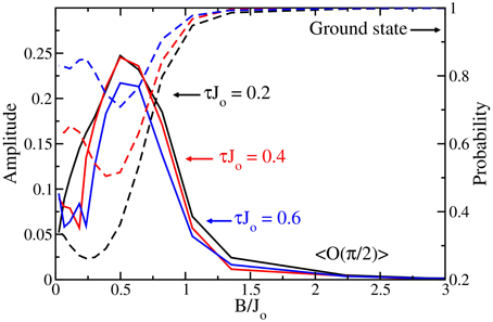
Figure 10. Amplitude of the oscillations when the transverse-field Ising model is held at different B∕J_o for 3 different τ = 0.2 (black), 0.4 (red), and 0.6 (blue), (where the arrows point toward the appropriate vertical axis; solid lines are the amplitude of oscillations, axis on the left and dashed lines are the ground-state probability, axis on the right). Before the minimum energy gap, the oscillations increase as the probability of the ground state decreases. However, after the minimum energy gap is passed, depletion of the excited states back to the ground state occurs and the amplitude of the oscillations decrease accordingly. This depletion is difficult to detect by measuring the amplitude of the oscillations at only one time.

3. Conclusion

We analyzed the amplitude of the oscillations for a given time-dependent Hamiltonian that is held constant for a time interval t_meas. to extract information about the ground-state probability. We demonstrated this analysis for the Landau-Zener problem and for the transverse-field Ising model (as would be simulated in the linear Paul trap). In both of the Hamiltonians, the amplitude of the oscillations becomes a maximum at a particular probability of the ground state and decreases as the ground-state probability either increases or decreases. Hence a single measurement of the amplitude cannot determine which side of the maximum one is on. Therefore, multiple measurements must be made where the amount of excitations are varied. Additionally as the probability of the ground state approaches 1, the amplitude decreases to 0 which can be difficult to measure given experimental noise.

We have described the simplest analysis one can do to extract information about the probability of the ground state. This approach can be refined by using signal processing techniques like compressive sensing to determine the Fourier spectra of the excitations. By monitoring the change of the weights of the delta functions, one can produce more accurate quantitative predictions for the probability of the ground state, because we can directly measure $P_1^{*}{P}_m\langle 1|\widehat{{O}}|m\rangle$ for a few different m-values. But this goes beyond the analysis we have done here.

For the transverse-field Ising model, de-excitations are observed, and were reflected in the amplitude of oscillations. However, after the minimum energy gap, more diabatic excitation can be created, but it is difficult to distinguish between the de-excitations and excitations. One interesting aspect is that as long as the ground-state probability remains high enough, measuring the height of the oscillation amplitude can be used to optimize the ground-state probability as a function of parameters used to determine the time-evolution of the system. This can be a valuable tool for optimizing the adiabatic state preparation protocol over some set of optimization parameters. But caution is needed to completely carry this out because the dependence of the ground-state probability on the oscillation amplitude is complex for complicated quantum systems and care is needed to be able to unambiguously carry out this procedure and achieve semiquantitative estimates of the ground-state probability.

Conflict of Interest Statement

The authors declare that the research was conducted in the absence of any commercial or financial relationships that could be construed as a potential conflict of interest.

Acknowledgments

JF and BY acknowledge support from the National Science Foundation under grant number PHY-1314295. JF also acknowledges support from the McDevitt bequest at Georgetown University. BY acknowledges support from the Achievement Rewards for College Students Foundation.

References

1. Feynman RP. Simulating physics with computers. Int J Theory Phys. (1982) 21:467–88. doi: 10.1007/BF02650179

CrossRef Full Text

2. Abrams DS, Lloyd S. Quantum algorithm providing exponential speed increase for finding eigenvalues and eigenvectors. Phys Rev Lett. (1999) 83:5162–5. doi: 10.1103/PhysRevLett.83.5162

CrossRef Full Text | Google Scholar

3. Britton JW, Sawyer BC, Keith AC, Wang CCJ, Freericks JK, Biercuk MJ, et al. Engineered two-dimensional Ising interactions in a trapped-ion quantum simulator with hundreds of spins. Nature (2012) 484:489–92. doi: 10.1038/nature10981

PubMed Abstract | CrossRef Full Text | Google Scholar

4. Senko C, Smith J, Richerme P, Lee A, Campbell WC, Monroe C. Coherent imaging spectroscopy of a quantum many-body spin system. Science (2014) 345:430–3. doi: 10.1126/science.1251422

PubMed Abstract | CrossRef Full Text | Google Scholar

5. Lanyon BP, Hempel C, Nigg D, Müller M, Gerritsma R, Zähringer F, et al. Universal digital quantum simulation with trapped ions. Science (2011) 334:57–61. doi: 10.1126/science.1208001

PubMed Abstract | CrossRef Full Text | Google Scholar

6. Shabani A, Mohseni M, Lloyd S, Kosut RL, Rabitz H. Estimation of many-body quantum Hamiltonians via compressive sensing. Phys Rev A (2011) 84:012107. doi: 10.1103/PhysRevA.84.012107

CrossRef Full Text | Google Scholar

7. Yoshimura B, Campbell WC, Freericks JK. Diabatic-ramping spectroscopy of many-body excited states. Phys Rev A (2014) 90:062334. doi: 10.1103/PhysRevA.90.062334

CrossRef Full Text | Google Scholar

8. Donoho DL. Compressed sensing. Inform Theory IEEE Trans. (2006) 52:1289–306. doi: 10.1109/TIT.2006.871582

PubMed Abstract | CrossRef Full Text | Google Scholar

9. Crank J, Nicolson P. A practical method for numerical evaluation of solutions of partial differential equations of the heat-conduction type. Adv Comput Math. (1996) 6:207–26. doi: 10.1007/BF02127704

CrossRef Full Text | Google Scholar

10. Torrontegui E, Ibez S, Mart-nez-Garaot S, Modugno M, del Campo A, Gury-Odelin D, et al. Shortcuts to adiabaticity. In: E. Arimondo, P. R. Berman and C. C. Lin, editors. Advances in Atomic, Molecular, and Optical Physics. Vol. 62. Oxford: Academic Press (2013). pp. 117–69.

11. Islam R, Senko C, Campbell WC, Korenblit S, Smith J, Lee A, et al. Emergence and frustration of magnetism with variable-range interactions in a quantum simulator. Science (2013) 340:583–7. doi: 10.1126/science.1232296

PubMed Abstract | CrossRef Full Text | Google Scholar

12. Zhu SL, Monroe C, Duan LM. Trapped ion quantum computation with transverse phonon modes. Phys Rev Lett. (2006) 97:050505. doi: 10.1103/PhysRevLett.97.050505

PubMed Abstract | CrossRef Full Text | Google Scholar

13. Kim K, Chang MS, Korenblit S, Islam R, Edwards EE, Freericks JK, et al. Quantum simulation of frustrated ising spins with trapped ions. Nature (2010) 465:590–3. doi: 10.1038/nature09071

PubMed Abstract | CrossRef Full Text | Google Scholar

14. Wang CCJ, Freericks JK. Intrinsic phonon effects on analog quantum simulators with ultracold trapped ions. Phys Rev A (2012) 86:032329. doi: 10.1103/PhysRevA.86.032329

CrossRef Full Text | Google Scholar