A Comprehensive Cold Gas Performance Study of the Pocket Rocket Radiofrequency Electrothermal Microthruster

This paper presents computational fluid dynamics simulations of the cold gas operation of Pocket Rocket and Mini Pocket Rocket radiofrequency electrothermal microthrusters, replicating experiments performed in both sub-Torr and vacuum environments. This work takes advantage of flow velocity choking to circumvent the invalidity of modeling vacuum regions within a CFD simulation, while still preserving the accuracy of the desired results in the internal regions of the microthrusters. Simulated results of the plenum stagnation pressure is in precise agreement with experimental measurements when slip boundary conditions with the correct tangential momentum accommodation coefficients for each gas are used. Thrust and specific impulse is calculated by integrating the flow profiles at the exit of the microthrusters, and are in good agreement with experimental pendulum thrust balance measurements and theoretical expectations. For low thrust conditions where experimental instruments are not sufficiently sensitive, these cold gas simulations provide additional data points against which experimental results can be verified and extrapolated. The cold gas simulations presented in this paper will be used as a benchmark to compare with future plasma simulations of the Pocket Rocket microthruster.

1. Introduction

In recent years, there has been a steady impetus in the satellite industry toward miniaturized microsatellites and microspacecraft, primarily driven by the desire to reduce spacecraft mass in order to reduce launch costs. This has led to the development of micro- (≤ 100 kg), nano- (≤ 10 kg), and picosatellites (≤ 1 kg), where the dramatic reduction in cost increases the accessibility to space, and brings with it the possibility of funding more missions and more frequent launches. The QB50 mission [1, 2] is an example of a scientific endeavor enabled by the affordability of CubeSats—a type nanosatellite made up of multiples of 1 kg, 10-cm cubic units. The mission employs a network of 50 CubeSats, built by university teams all over the world, to study the lower thermosphere. It also demonstrates the possibility of using a large fleet of low-cost microspacecraft to reduce mission risk by distributing functionality and incorporating redundancy, where the loss of one or even multiple microspacecraft will not jeopardize the entire mission.

The rise in popularity of microspacecraft has in turn produced a strong interest and demand in the development of micropropulsion devices. These devices must meet the unique propulsion needs of each specific mission, which may include attitude control, orbital station-keeping, drag compensation to slow orbital decay, de-orbit manoeuvres, or constellation formation and maintenance. At the same time, micropropulsion devices must also adhere to the stringent design requirements imposed due to severe mass, volume, and power constraints of the microspacecraft.

Two main classes of propulsion technologies have been envisioned and flown for spacecraft. The first is gas and chemical propulsion, which ranges from the traditional or microelectromechanical systems-based (MEMS) cold gas thrusters [3], to warm gas and chemical propellant systems. The second is electric propulsion, which can be grouped into three distinct categories: electrothermal, electrostatic, and electromagnetic. Electrothermal propulsion includes devices like arcjets [4–6], resistojets [7], hollow cathode thrusters [8, 9], and the Pocket Rocket microthruster [10] which is the subject of this paper. Electrostatic propulsion has been dominated by a large variety of gridded ion thrusters, the most recent developments including NASA's annular-geometry ion engine (AGI-Engine) [11, 12] and the NASA evolutionary xenon thruster (NEXT) [13, 14], but also include experimental technologies like the field emission electric propulsion (FEEP) concept [15] and its precedent colloid thrusters. Finally, electromagnetic propulsion boasts the mature Hall-effect thruster [16] and its variants [17–19], as well as newer technologies like magnetoplasmadynamic (MPD) thrusters [20, 21] and ablative pulsed plasma thrusters (PPTs) [22]. For more information, a comprehensive review of electric propulsion is available in Charles [23] and Mazouffre [24], while Micci and Ketsdever [25] and Scharfe and Ketsdever [26] compiles a review of both classes of propulsion technologies with a specific focus on micropropulsion for microspacecraft.

2. Outline

This paper presents computational fluid dynamics simulations of the cold gas operation of Pocket Rocket and Mini Pocket Rocket radiofrequency electrothermal microthrusters, replicating experiments performed in both sub-Torr and vacuum environments. The simulations are performed using the commercial CFD-ACE+ multiphysics package, chosen for its ability to model plasmas in addition to fluids. The cold gas simulations presented in this paper will be used as a benchmark to compare with future plasma simulations of the Pocket Rocket microthruster.

The following section will introduce the Pocket Rocket microthruster experiment with reference to previously published results, and subsequent sections will discuss the reasons for using a fluid simulation technique over other techniques before detailing the Pocket Rocket simulation mesh and the parameters used for the simulations. The main results of the cold gas simulations are presented in the results and discussion section, along with a theoretical definition and discussion of concepts such as flow velocity choking, thrust and specific impulse, as well as the boundary layer friction force.

The list of the simulations presented in this paper is as follows. The first set of simulations “PR laboratory condition” is a direct representation of the PR experiment, performed for the purpose of verifying the correct simulation parameters and settings required to reproduce experimental results. The second set of simulations “PR nozzle choked flow condition” is performed using a PR mesh which is slightly modified to incorporate a converging-diverging nozzle. This is aimed at validating the treatment of flow velocity choking in CFD-ACE+, and its ability to handle the simulation of vacuum in the downstream region (by setting the outlet pressure to zero) without compromising the results in the other upstream regions. The third set of simulations “PR vacuum condition” models the performance of PR in a vacuum environment, and provides thrust results that are otherwise currently unobtainable from experiment. Finally, the fourth set of simulations “MiniPR vacuum condition” is a direct representation of the MiniPR experiment performed in the Wombat space simulation chamber [27]. The simulated thrust is compared to the experimentally measured values and the theoretical expectation in order to verify the reliability of the results obtained by simulation. The main results of the simulations are summarized in Table 1.

TABLE 1

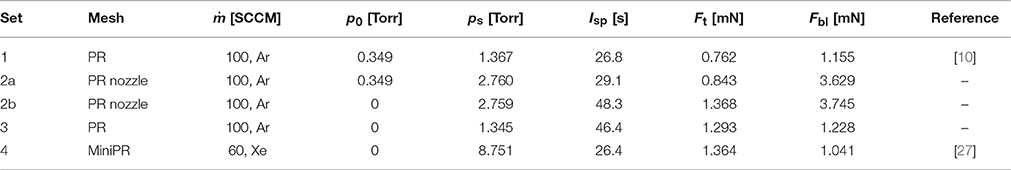
Table 1. Summary of the main simulation results for selected flow rates and set outlet pressure: plenum stagnation pressure, specific impulse, total cold gas thrust, boundary layer friction force, and references to related experiments.

3. Pocket Rocket Microthruster Experiment

Pocket Rocket (PR) is a radiofrequency plasma electrothermal microthruster currently under development by the Space Plasma, Power, and Propulsion (SP3) Laboratory at the Australian National University. The specifications of PR have been previously described in depth in Charles and Boswell [10] and Greig [28]. The detailed dimensions and geometry of PR are specified later in the description of the PR simulation mesh. In summary, PR (Figure 1) primarily consists of an annular electrode fitted coaxially around the middle section of an alumina (Al₂O₃) tube (hereafter called the plasma cavity or discharge volume), through which a propellant gas is puffed. PR can operate with a wide range of gas propellants, but performs best with monatomic inert gas propellants such as Ar and Xe. The propellants may be stored either in a pressurized vessel or in a solid form (e.g., I₂). In the laboratory, a mass flow controller regulates a steady flow of gas into PR. In a microspacecraft, this function may be performed by a combination of a pressure regulator and a solenoid valve, or by MEMS devices. Overall, the construction of PR is lightweight, simple, and robust, and can be manufactured at low cost.

FIGURE 1

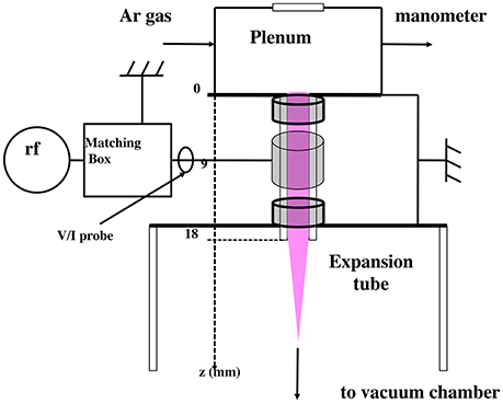
Figure 1. Schematic of the Pocket Rocket experiment showing the plasma operation mode with Ar propellant.

Radiofrequency (RF) power (typically 13.56 MHz) supplied to the electrode will ignite a plasma in the discharge volume. The amount of power required to provide sufficient voltage to ignite a plasma varies depending on the Paschen minimum of the propellant gas. In PR, breakdown of Ar gas occurs within 10⁻⁴ s [29, 30] and is achievable with only a few watts of power, which can be supplied from small solar panels or batteries on board a microspacecraft. For normal low power operation, there is no concern for wear, corrosion, or thermal fatigue on PR. Unlike gridded ion thrusters and Hall-effect thrusters, no neutralizer is necessary as the ions and electrons in the PR plasma exit the microthruster together along with the neutral gas propellant. This is advantageous as the lifetime of most electrostatic and electromagnetic thrusters is limited by the lifetime of the neutralizer and other plasma-facing components.

Depending on the amount of RF power supplied (0.1–50 W), the plasma heats the gas to temperatures in excess of 1000 K [30–33] by depositing power directly into the propellant, thereby enhancing thrust production over cold gas performance levels, with minimal increase in thruster complexity. By controlling the propellant flow rate and the RF power in continuous or pulsed operation, PR can produce precisely manipulable thrust on the milliNewton-scale.

The PR experimental apparatus has been previously described in Charles and Boswell [10]. Presently, PR is attached to a glass expansion tube (d = 4.5 cm, l = 10 cm), and mounted to one face of a 20-L six-way cross vacuum chamber (d = 20 cm, l = 40 cm) in which a base pressure of ≤ 1 mTorr is achieved with a scroll pump. A 10-Torr capacitance manometer is used to measure the static pressure of the gas inside the plenum of PR, while a Pirani gauge and another capacitance manometer tracks the pressure in the chamber. The mass flow controller used in the PR experimental setup is calibrated for 100 SCCM of N₂, and equivalently 144 SCCM of Ar, which has a theoretical gas correction factor (GCF) of 1.44. Increasing the flow rate of the selected gas into PR from 0 SCCM to the full scale increases the pressure in both the plenum and the chamber. At the maximum pumping rate, the ratio of the PR plenum pressure to the chamber pressure is about 4 : 1, primarily dependent on the diameter and length of the discharge volume and the expansion tube, and secondarily on the species of gas. In earlier experiments [30–33], the pressure ratio was maintained at 2 : 1 by limiting the pumping rate.

Mini Pocket Rocket (MiniPR), previously described in Charles et al. [27, 34, 35], is a variation of the PR microthruster with a narrower discharge volume. For thrust experiments [27], MiniPR is mounted on a pendulum thrust balance inside a 1700-L cylindrical space simulation chamber (d = 1 m, l = 2.2 m), evacuated to a base pressure of ≤ 10⁻⁶ Torr by a series of scroll, turbomolecular, and cryogenic pumps. Performing cold gas and plasma thrust measurement experiments of this nature is challenging due to the current prototype design of MiniPR (and PR), as the gas propellant and the RF power must be routed to the microthruster from external sources. The gas line and the RF cable used for this purpose introduce mechanical resistance, which can be slightly alleviated by anchoring them to the thrust balance. Similar challenges were observed in Böhrk and Auweter-Kurtz [6], in which they opted to use indirect measurement methods employing a baffle plate and a Pitot probe. A solution would be to use integrated autonomous propellant and RF subsystems on the microthruster. However, as such a system is not yet available, simulation of the microthruster is able to produce more accurate thrust results than experiments at the present time.

4. CFD-ACE+ Simulation

The Knudsen number Kn is a dimensionless parameter which determines whether a flow is better characterized by continuum or statistical mechanics, defined as the ratio of the mean free path λ of a molecule to the characteristic length of the flow system (i.e., the radius of the plenum, discharge volume, and expansion tube). The mean free path is defined as:

$\begin{array}{ll}\lambda =\frac{k_{\mathrm{\text{B}}}T}{\sqrt{2}\pi D^{2}p}& (1)\end{array}$

where $k_{\mathrm{\text{B}}}=1.38064852\times 10^{-23}\mathrm{\text{J}}·{\mathrm{\text{K}}}^{-1}$ is the Boltzmann constant, T and p are the local temperature and static pressure respectively, and D is the Lennard-Jones length or collision diameter of the chosen molecule. This paper uses the kinetic mean free path instead of the fluid mean free path which is calculated with the fluid dynamic viscosity, as the former definition preserves its accuracy even in high Kn flows.

Generally, computational fluid dynamics (CFD) simulations are limited to modeling continuum regime flow (Kn ≲ 0.01), and the treatment of rarefied flows with higher Knudsen numbers require techniques such as molecular dynamics (MD) or direct simulation Monte Carlo (DSMC). However, MD simulations are extremely computationally expensive for all but very small systems as it scales by the square of the number of molecules involved. A more practical solution is DSMC simulations, which use a characteristic particle to represent a large ensemble of real molecules. While this reduces the scale of the problem, DSMC simulations are nevertheless still very much more computationally expensive than CFD simulations for modeling weakly rarefied flows, particularly in the continuum (Kn ≲ 0.01) and slip (0.01 ≲ Kn ≲ 0.1) regimes. Typically, studies seeking to model flows spanning a wide range of Knudsen numbers resort to a hybrid CFD/DSMC approach, applying CFD techniques to regions of low Kn, and using the results obtained thus as a boundary condition for the neighboring regions of high Kn where DSMC techniques are employed [36].

This paper presents CFD cold gas simulations of the PR and MiniPR microthrusters performed with the commercial CFD-ACE+ multiphysics package. For the purposes of this work, DSMC techniques are not required as the primary interest is in modeling the low-Kn internal regions of the microthrusters. This work takes advantage of the flow velocity choking phenomenon to circumvent the invalidity of modeling vacuum regions within a CFD simulation, while still preserving the accuracy of the desired results in the internal regions of the microthrusters. The flow velocity choking phenomenon will be further discussed in detail later in the text.

Flow velocity choking is a compressible flow effect. Modeling compressible flows in CFD-ACE+ requires the flow and heat transfer simulation modules. The flow module numerically solves the Navier-Stokes equations for the flow velocity and pressure field over a given meshed geometry. The simulation volume is discretized and the continuity equations numerically integrated over each cell via the finite volume method. The result is assigned to the cell center, and interpolated to the cell faces to determine the flux across each cell interface. Mass conservation is implemented, and pressure is calculated using the iterative SIMPLEC algorithm until convergence. Fixed value boundary conditions (e.g., inlets, outlets, isothermal walls) are imposed by setting a source term in a fictitious cell on the external boundary of the volume, while zero-flux boundary conditions (e.g., symmetric boundaries, adiabatic walls) are achieved simply by setting the cell interface coefficients to zero. Most importantly, the heat transfer module keeps track of energy transfers arising from work done on and by the gas during compression and expansion, as well as to impose thermal boundary and initial conditions. Energy conservation is implemented via the total enthalpy equation, and solved similarly to those described above. The simulations are self-consistent, with no artificial source terms or limits used.

The key advantage of simulations is the ability to generate a complete three-dimensional picture of all the measurable variables. This presents a valuable edge over experiments, especially in the field of microthrusters, which due to their small geometry can be difficult or not feasible to access with ordinary instruments. The results of the cold gas simulations presented in this work will be compared with published cold gas thrust measurement experiments [27] and theoretical expectations to establish their validity and accuracy. The cold gas performance results of PR will be used as a benchmark for future plasma operation studies to be performed also in CFD-ACE+.

4.1. Pocket Rocket Simulation Mesh

The two-dimensional simulation mesh for PR is shown in Figure 2. It is axisymmetric, and represents the top-half cross section of the microthruster. The mesh is divided into four main regions, which include three fluid volumes: the plenum (r = 20 mm, l = 12 mm), discharge volume (r = 2.1 mm, l = 18 mm), and downstream (l = 51 mm), and one solid volume being the cavity wall (Δr = 1.0 mm, l = 18 mm). Rotating the mesh about the horizontal axis of symmetry renders the cylindrical geometry of PR and a hemispherical downstream region. The total number of cells in the PR mesh is 25405; the MiniPR mesh has 22525 cells, given its narrower discharge volume (r = 0.8 mm) and thinner cavity wall (Δr = 0.7 mm), but is otherwise identical to the PR mesh. Most of the simulation studies of this work are performed using the PR mesh, as the higher number of cells across the radius of the discharge volume (21 vs. 8 in the MiniPR mesh) is beneficial for the accuracy and resolution of the simulations.

FIGURE 2

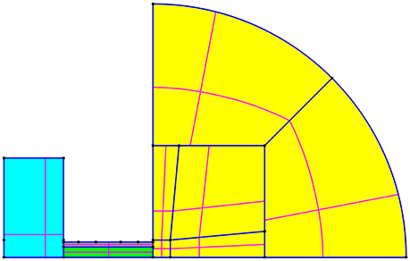
Figure 2. Two dimensional cross section of the axisymmetric top half of the PR mesh, with the four regions: plenum (cyan), discharge volume (green), downstream (yellow), and cavity wall (gray). Blue lines denote the interfaces between adjacent regions or subregions. The magenta lines show the position of the median cell in each region or subregion. The inlet is defined to be the cylindrical surface of revolution formed by the top edge of the plenum, and the outlet is the hemispherical surface on the far right of the downstream region. The front plenum wall is defined to be the left internal face of the plenum region, while the rear plenum wall is the right internal face of the plenum region surrounding the entrance to the discharge volume region.

The discharge volume is the region of primary interest, and features a uniform orthogonal square grid consisting of 0.1 × 0.1 mm cells. The cavity wall region and the first adjacent downstream subregion also have the same-sized cells. The cells in the plenum region smoothly increase in size with increasing distance from the discharge volume region (up to 0.5 × 0.5 mm in the top left corner). Orthogonality and zero skew are maintained in these regions for compatibility with the CFD-ACE+ plasma module, which will be used for plasma CFD simulations in the future. The grids of the remaining downstream subregions smoothly increase in size with increasing distance from the first downstream subregion. There is some unavoidable skew as the shape of the grid transitions from a square to a quadrant. This is acceptable as the plasma studies will mainly be performed in the upstream regions. As for the boundaries, the inlet is defined to be the cylindrical surface of revolution formed by the top edge of the plenum, and the outlet is the hemispherical surface on the far right of the downstream region. Walls enclose the remaining external edges of the mesh. Interfaces exist between adjacent regions, allowing the two regions to communicate information.

There are several reasons for choosing a hemispherical shape for the downstream region. The downstream region represents either the experimental expansion tube, vacuum chamber, or space. When the Knudsen number is not too high (Kn ≲ 0.1), the results of the simulation is insensitive to the shape of the downstream region, and thus the mesh need not exactly reproduce the experiment apparatus (e.g., the expansion tube). On the other hand, when modeling vacuum in the downstream region (e.g., in the 1700-L space simulation chamber), fluid dynamics become invalid as the flow enters the transitional (0.1 ≲ Kn ≲ 10) and free molecular regimes (Kn≳10). To mitigate unphysical behavior, the vacuum outlet boundary has to be placed a sufficient distance away from the important regions of the simulation. A hemispherical outlet boundary is equidistant from the exit of discharge volume and isotropic, eliminating the directional bias and circulation effects that arise from having boundaries at unequal distances, as well as computational anomalies caused by corners. These are problems that would arise if a cylindrical mesh were used for the downstream region. To accommodate the hemispherical outlet boundary, the downstream region is divided into six subregions that are designed to allow for optimal smooth expansion of cells in both radial and polar directions with minimal skew.

4.2. Simulation Parameters

In order to produce realistic and accurate results, it is imperative that the correct boundary and volume conditions are applied. The boundary conditions refer to the flow and heat properties at the boundaries of each region of the simulation mesh. For each simulation, a fixed mass flow rate of the gas is specified at the inlet. The temperature of the incoming gas is set at 300 K, and the pressure at the inlet is calculated automatically as the simulation progresses. At the outlet, a fixed pressure is specified, with the value of either the experimentally measured chamber pressure or zero depending on the investigation. The temperature of the backflow gas is set at 300 K for the former case, and is irrelevant for the latter case. The inlet mass flow rate and the outlet pressure are the only independent variables in the simulations.

For the simulations presented in this paper, the walls (front and rear plenum walls, external cavity wall, and the downstream wall) are set to be isothermal, with the temperature fixed at 300 K to reproduce laboratory conditions. The gas-facing surfaces (front and rear plenum walls, internal cavity wall, and the downstream wall) are defined to be zero-flux boundaries with either inviscid, no-slip, or slip boundary conditions depending on the investigation.

The flow boundary condition is one of the most influential parameters affecting the flow behavior in the PR and MiniPR simulations. Due to the small size of microthrusters, the large surface area to volume ratio of the flow system and a nonnegligible Knudsen number mean that the boundary layer accounts for a significant portion of the flow system, and effectively dictates the behavior of the main flow. In microthrusters and other systems operating in the slip regime where the Knudsen number is in the range of 0.01 ≲ Kn ≲ 0.1, the solution to the Navier-Stokes equations are only valid in the main flow and not in the boundary layer. In this regime, it is necessary use the slip boundary condition, where the interaction between the gas molecules and the wall is characterized by an accommodation coefficient α, a number between 0 and 1.

The tangential momentum accommodation coefficient (TMAC) α_u was first introduced by Maxwell [37] to describe the nature of the reflection of a molecule off a wall: α_u = 0 represents specular reflection, while α_u = 1 represents diffusive reflection. In reality, molecular reflection is a mixture of diffuse and specular reflection, with the exact value of α_u dependent on the species of gas. Measurements of α_u are typically performed by tracking the flow of gas through a microchannel. These experiments [38–46] are performed over a wide range of pressures at room temperature, and use microchannels with different shapes and diameters, constructed of various materials and surface treatments. Since the α_u of each gas remains roughly constant across different conditions and flow regimes, it is justified to use the mean value of α_u for each gas in the simulations.

Similar to the concept of the TMAC, the original formulation of the thermal accommodation coefficient (TAC) α_T is attributed to Smoluchowski von Smolan [47]. In general, α_T is not the same as α_u for each gas species. α_T is measured experimentally [48–53] using a variety of techniques often involving two walls held at different temperatures. While α_T is roughly constant for each gas across different surface materials and roughnesses, it appears to decrease as the temperature difference between the two walls increases [54]. However, due to the lack of extensive studies [55] on this behavior, the mean value from Vargaftik [48], Porodnov and Kulev [49], Song and Yovanovich [50], Rader et al. [51], Ganta et al. [52], and Trott et al. [53] is used for each gas in the simulations.

Using the slip boundary condition produces the correct solution for the main flow, but at the cost of introducing a fictitious slip velocity and temperature jump at the wall, which come about as a result of extrapolating the Navier-Stokes solution from the correct main flow solution to the boundary layer. Since the primary interest is in the main flow, it is more important to obtain accurate results there than at the wall. For most cases where α is high, the aberrations in the solution arising from the slip velocity and temperature jump are relatively small, and can be tolerated. Kogan [56] presents a cogent explanation for the necessity of slip boundary conditions for treating flows at small Knudsen numbers. A primer on the compressible Navier-Stokes equations, accommodation coefficients, and the slip velocity and temperature jump boundary conditions can be found in Karniadakis et al. [57].

The volume conditions refer to the material properties of the fluid (N₂, Ar, and Xe gas) and the solid (Al₂O₃) used in the simulations. For the former, CFD-ACE+ contains a database of elemental and molecular species with their respective atomic or molecular mass available by default. The Lennard-Jones length or collision diameter for each species is entered into the database using values from Poling et al. [58]. It is also necessary to input values for the isobaric specific heat, thermal conductivity, and dynamic viscosity of each gas species. These parameters are obtained from the NIST Thermophysical Properties of Fluid Systems database [59] as a piecewise linear function of temperature (in increments of 1 K from the boiling point) at a constant pressure of 1 Torr (as PR and MiniPR operate in the 0–10 Torr range). The mass diffusivity data of the each gas species are collected from Amdur and Mason [60], Amdur and Schatzki [61], Dymond [62], Hutchinson [63], Winn [64], and Winter [65], wherein the values are quoted for atmospheric pressure (760 Torr). For self-diffusion in gases, the empirical relation D ∝ p⁻¹ [66] is used to calculate the respective values for 1 Torr. A fifth-order Maclaurin series in temperature is fitted to the 1-Torr mass diffusivity data, and the polynomial coefficients are entered into the CFD-ACE+ database. Finally, while it is possible to input the density using a piecewise linear function of temperature as before, the ideal gas law is used instead due to the requirements for modeling compressible flows. As for solid materials, similar parameters that are required are obtained from sources like [67, 68].

5. Results and Discussion

5.1. Set 1: PR Laboratory Condition

The main input for the CFD cold gas simulations is the inlet flow rate of the selected gas and the outlet pressure. The first set of simulations with the PR mesh was ran with 25–144 SCCM of Ar and 25–100 SCCM of N₂ (to verify the calibration of the mass flow controller GCF for Ar), and the outlet pressure of each case is set to the experimentally measured chamber pressure. Figure 3 plots the PR experimental plenum pressure (blue line) and chamber pressure measurements (black line) for Ar. Also plotted are the simulated plenum pressure using inviscid (magenta crosses), no-slip (magenta plusses), and slip boundary conditions with various accommodation coefficients (circles) for Ar. The results for N₂ are very similar, and not discussed here.

FIGURE 3

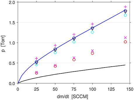
Figure 3. Experimental plenum pressure (blue line) and chamber pressure (black line) measurements against mass flow rate of Ar into PR. Set 1: Simulated plenum pressure using inviscid (magenta crosses), no-slip (magenta plusses), and slip boundary conditions with α_u = 0 (red circles), α_u = 0.5 (cyan circles), and α_u = 0.9 (blue circles). Set 3: α_u = 0.9 (black triangles).

It is found that the simulated plenum pressure matches the experimental plenum pressure only when a slip boundary condition is used with the recommended value of α_u = 0.9 for both N₂ and Ar [38–46]. The plenum pressure is very slightly overestimated with a no-slip boundary condition, and severely underestimated with an inviscid boundary condition. Using α_u = 0 produces results similar to the inviscid case, as expected. Notably, α_u = 0.5 gives only slight underestimates, while the results for α_u = 1 (not shown for clarity) is almost indistinguishable from that of α_u = 0.9. This is expedient, as it means that the simulations are insensitive to small errors in α_u for values close to 1.

The plenum pressure is a very unambiguous and spontaneous indicator of the flow characteristics in PR. For the experimental 100 SCCM Ar case, the steady state plenum pressure is measured to be 1.365 Torr, while the chamber pressure is at 0.349 Torr. For reference, the simulated steady state pressure profile (solid blue line) of the α_u = 0.9 case, which matches the experiment best, is plotted in Figure 4.

FIGURE 4

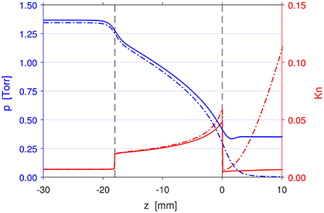
Figure 4. Axial profiles of the pressure (blue) and Knudsen number (red) at r = 0 mm for the 100 SCCM Ar PR simulations in Set 1 (solid lines) and Set 3 (dash-dotted lines). −30 mm ≤ z < −18 mm is the plenum, −18 mm ≤ z ≤ 0 mm is the discharge volume, and z > 0 mm is the downstream region.

The experiment begins in the initial state where the whole system is at the base pressure of ≤ 1 mTorr. Immediately after the mass flow controller is turned on, Ar gas entering the system causes the pressure to increase in the plenum, thereby setting up a small pressure difference between the plenum and the chamber. The pressure difference is bridged by the discharge volume, which tries to balance the pressure on both ends by moving gas from the plenum where the pressure is higher to the chamber where the pressure is lower. However, the rate at which the gas can be moved is dependent on the steepness of the pressure gradient. In the beginning while the pressure difference is still small, the flow rate through the discharge volume will be less than the imposed flow rate into the plenum. Consequently, the pressure in the plenum will continue to increase until the pressure gradient in the discharge volume can support the full flow rate, at which point the system attains equilibrium. This happens on the time scale of about 10 s.

While it is possible to model the temporal evolution of the cold gas flow in PR from the initial state with CFD-ACE+, the normal operation of PR is in the steady state with constant gas flow. The simulated steady state axial velocity profile (solid blue line) is plotted in Figure 5 along with the local sound speed (solid red line), calculated using the equation:

$\begin{array}{ll}{c}_{\mathrm{\text{s}}}=\sqrt{\frac{\gamma k_{\mathrm{\text{B}}}T}{m}}& (2)\end{array}$

where γ is the adiabatic index, $k_{\mathrm{\text{B}}}=1.38064852\times 10^{-23}\mathrm{\text{J}}·{\mathrm{\text{K}}}^{-1}$ is the Boltzmann constant, T is the local temperature of the gas, and m is the atomic mass of the gas. As the plenum has a much larger diameter than the discharge volume, it acts as a reservoir where the pressure is constant throughout most of its volume, and the flow there is effectively stagnant. As the diameter of the system shrinks from the plenum to the discharge volume, there is an increase in the axial velocity accompanied with a decrease in the pressure due to the Venturi effect. In the discharge volume, the flow is further accelerated by the pressure gradient up to the local sound speed near the exit. Past the exit, the flow decelerates as it expands into the downstream region, where the pressure is at a constant 0.349 Torr.

FIGURE 5

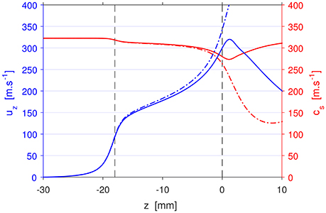
Figure 5. Axial profiles of the axial velocity (blue) and local sound speed (red) at r = 0 mm for the 100 SCCM Ar PR simulations in Set 1 (solid lines) and Set 3 (dash-dotted lines).

It can be seen from the Knudsen number profile (solid red line) in Figure 4 that for a pressurized downstream region which reproduces the laboratory conditions, the flow in the plenum and downstream regions are in the continuum regime (Kn ≲ 0.01) while the flow in the discharge region is in the slip regime (0.01 ≲ Kn ≲ 0.1). The flow characteristics in PR is dominated by the flow in the discharge region, and hence ultimately dictated by the slip regime flow behavior. This substantiates the necessity of using the correct slip boundary conditions and α_u for modeling PR and other systems operating in the slip regime.

5.2. Flow Velocity Choking

Before proceeding to the CFD simulations involving vacuum regions, it is firstly necessary to examine the theory of flow velocity choking. Consider isentropic flow of a compressible fluid through a stream tube. Assume that the cross-sectional area of the stream tube varies sufficiently slowly with distance along the z-axis, so that the flow depends only on the distance along the stream tube and is approximately one-dimensional. Then, from using Bernoulli's equation, the conservation of mass, and the isentropic flow relations [69], the variation in the axial velocity of the flow du_z/u_z can be related to the variation of the cross-sectional area dA/A by:

$\begin{array}{ll}\frac{\mathrm{\text{d}}{u}_z}{u_z}=\frac{1}{{\mathrm{\text{Ma}}}^2-1}·\frac{\mathrm{\text{d}}A}{A}& (3)\end{array}$

where Ma = u_z/c_s is the Mach number, defined as the ratio of the axial velocity u_z to the local sound speed c_s.

Equation (3) reveals that when the flow is subsonic (Ma < 1), a decrease in A will result in an increase in u_z (du_z ∝ −dA). Conversely, when then flow is supersonic (Ma > 1), increasing A will also increase u_z (du_z ∝ dA). At the critical state of Ma = 1, dA/A must necessarily be zero. This means that either the flow must expand into an infinite area, or that the cross-sectional area of the stream tube must be at a minimum, i.e., at the vena contracta. This fact is of great significance in high speed flows, as it dictates that a subsonic flow cannot be accelerated to supersonic speed without first having satisfied either of the aforementioned conditions. Hence, for a converging nozzle, the maximum flow velocity attainable will be the local sound speed, occurring at the exit. To achieve supersonic flow, a converging-diverging nozzle is required. The convergent section of the nozzle accelerates the subsonic flow, which then attains the local sound speed when the cross-sectional area narrows to the minimum at the throat. Thereafter, the divergent section of the nozzle further accelerates the sonic flow to supersonic speed.

As discussed in the previous section, the acceleration of the flow is directly related to the pressure gradient. If the pressure gradient is insufficiently steep, the flow will not become sonic. Thus, there is a minimum pressure difference across the vena contracta required for achieving sonic flow. For a polytropic gas with the adiabatic index γ, the ratio of the stagnation pressure p_s upstream of the vena contracta to the critical downstream pressure $p_0^{*}$ required for achieving sonic flow is given by:

$\begin{array}{ll}\frac{p_{\text{s}}}{p_0^{*}}={\left(\frac{\gamma +1}{2}\right)}^{\frac{\gamma }{\gamma -1}}& (4)\end{array}$

Equation (4) is exact only if the pressure difference occurs in the immediate vicinity of the vena contracta. In such case, the critical pressure ratio is 2.053 for a monatomic ideal gas with γ = 5/3, and 1.893 for a diatomic ideal gas with γ = 7/5. The critical pressure ratio varies almost linearly with γ, and is of the same order of magnitude for all gases ($p_{\mathrm{\text{s}}}/p_0^{*}~2$). When the critical pressure ratio is satisfied, the flow velocity attains the local sound speed at the vena contracta. Further decreasing the downstream pressure will not cause the flow velocity at the vena contracta to increase past the local sound speed, since Ma = 1, if it occurs, must occur at the vena contracta. This phenomenon is known as flow velocity choking. When the flow is choked, the flow conditions upstream of the vena contracta become insensitive to the flow conditions downstream.

In reality, the pressure drop is not immediate but instead manifests over a nonzero distance. In the example of PR, as shown in Figure 4, the pressure falls continuously along the entire length of the discharge volume. Hence, the critical pressure ratio given by Equation (4) cannot be used to determine if the flow velocity choking condition is met. For choked flow to occur, the pressure must fall sufficiently sharply in a local region, which is only possible if the stagnation pressure in the plenum is many times higher than the downstream pressure.

5.3. Set 2: PR Nozzle Choked Flow Condition

To demonstrate and to test the treatment of flow velocity choking in CFD-ACE+, the second set of simulations uses a slightly modified version of the PR mesh. The only difference between the original PR mesh and the mesh used in Set 2 is the introduction of a constriction at z = −3 mm to replicate a simple converging-diverging nozzle. The convergent section is at −6.5 mm < z < −3 mm, and the divergent section is at −3 mm < z < 0 mm. The diameter of the throat is 2.1 mm, half that of the discharge volume diameter, while the diameter of the exit is unchanged. The simulations in this set are run in pairs, one with the outlet pressure p₀ set to the experimentally measured outlet pressure p_c, and the other with p₀ = 0 Torr, with 25–144 SCCM of Ar.

Figure 6 illustrates the geometry of the Set 2 mesh, focusing in particular on the flow conditions through discharge volume and the converging-diverging nozzle. Displayed here are the simulations using 100 SCCM of Ar, with p₀ = 0.349 Torr (top) and p₀ = 0 Torr (bottom). The velocity magnitude is mapped in color, while the isocurves (black lines) represent Mach numbers 0.25, 0.5, 0.75, and 1. In both cases, the flow enters the discharge volume uniformly across most of the diameter, with a slow boundary layer near the wall. Before the nozzle, the velocity magnitude is much lower than Mach 0.25. As the cross-sectional area begins to decrease, the flow is accelerated very quickly in the short convergent section, up to close to the local sound speed at the throat. The actual Mach 1 sonic surface occurs very slightly behind the throat due to boundary layer effects. In the divergent section, the flow is further accelerated to supersonic speeds. In the p₀ = 0.349 Torr case however, the flow is almost immediately decelerated upon leaving the discharge volume as it encounters the static gas present in the downstream region.

FIGURE 6

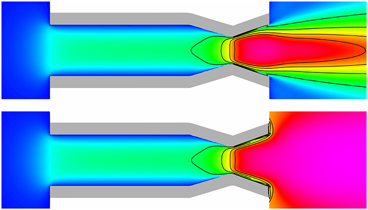
Figure 6. Set 2: PR nozzle using 100 SCCM of Ar, with p₀ = 0.349 Torr (top) and p₀ = 0 Torr (bottom). Velocity magnitude is mapped in color from 0 m·s⁻¹ (blue) to 527.9 m·s⁻¹ (magenta) in logarithmic scale, while the isocurves (black lines) represent Mach numbers 0.25, 0.5, 0.75, and 1. With a converging-diverging nozzle, the flow velocity becomes choked at the throat, and the flow conditions upstream are identical despite the large difference in downstream pressure.

Most importantly, Figure 6 shows that the flow velocity does indeed become choked at the throat of a converging-diverging nozzle. When the flow is choked, the flow conditions upstream of the throat are identical in the two cases despite the large difference in the downstream pressure. This behavior is consistent for the p₀ = p_c and p₀ = 0 Torr pairs of simulations for all the flow rates tested, with small differences in the exact position and shape of the sonic surface due to the different thicknesses of the boundary layer for different flow rates.

Figure 7 plots the plots the pressure (blue) and Knudsen number (red), and Figure 8 plots the axial velocity (blue) and sound speed (red) profiles on the central axis for the Set 2 100 SCCM Ar, p₀ = 0.349 Torr case (solid lines) and p₀ = 0 Torr case (dash-dotted lines). The respective parameters are congruent for both cases in the whole range from the front wall of the plenum at z = −30 mm, through the discharge volume and the converging-diverging nozzle, up to very near the exit.

FIGURE 7

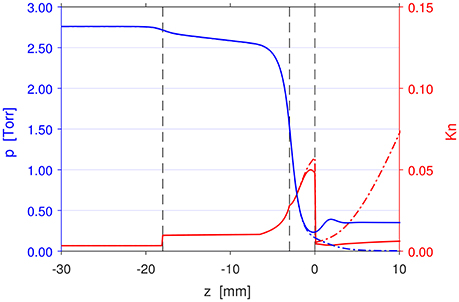
Figure 7. Axial profiles of the pressure (blue) and Knudsen number (red) at r = 0 mm for the PR simulations in Set 2 (Figure 6) with 100 SCCM Ar, p₀ = 0.349 Torr (solid lines) and p₀ = 0 Torr (dash-dotted lines). The throat of the nozzle is located at z = −3 mm.

FIGURE 8

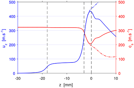
Figure 8. Axial profiles of the axial velocity (blue) and local sound speed (red) at r = 0 mm for the PR simulations in Set 2 (Figure 6) with 100 SCCM Ar, p₀ = 0.349 Torr (solid lines) and p₀ = 0 Torr (dash-dotted lines).

The plenum pressure in the Set 2 PR nozzle 100 SCCM Ar simulation is 2.760 Torr, about twice as high as the 100 SCCM Ar simulation from Set 1, due to the constriction of the discharge volume. With a converging-diverging nozzle, the pressure in the discharge volume remains high with only a very slight gradient through most of its length as distinct from the result in Set 1, and most of the pressure difference is dropped in the vicinity of the throat. For the present case, Equation (4) may be used to give a rough estimate of the critical downstream pressure required for sonic choked flow to occur. Finally, near the exit at z = 0 mm, the pressure in the p₀ = 0 Torr case decreases monotonically to zero to match the set outlet boundary condition. In the p₀ = 0.349 Torr case, the flow is slightly overexpanded in the divergent section of the unoptimized nozzle, and the pressure fluctuates slightly at z = 0–3 mm before settling to the downstream pressure.

As for the axial velocity (Figure 8), the increase in velocity due to the Venturi effect at the entrance of the discharge volume is smaller than in Set 1 (Figure 5), since the pressure in the discharge volume is similar to the plenum pressure. Also, the small pressure gradient in the discharge volume does not accelerate the flow, resulting in an almost constant axial velocity in the discharge volume. As discussed earlier, most of the acceleration takes place in the converging-diverging nozzle. Overall, the flow behavior in the PR nozzle simulations is consistent with the theory of flow velocity choking laid out in the previous section.

For the p₀ = 0 Torr cases in this set of simulations and hereafter, the high Knudsen number past z = 0 mm means that the results in the downstream region are not guaranteed to be valid and therefore should not be used for analysis. Even so, this set of simulations demonstrates that CFD-ACE+ is able to treat flow velocity choking correctly and reliably provides valid results in the regions upstream of z = 0 mm, even if the downstream region, which accounts for a significant volume of the simulation mesh, has Knudsen numbers higher than what CFD techniques usually allow.

5.4. Set 3: PR Vacuum Condition

Relying on the principles established by Set 2, the third set of simulations uses the original PR mesh, with 25–144 SCCM of Ar, α_u = 0.9, and the outlet pressure p₀ set to 0 Torr to model the performance of PR in vacuum. Figures 4, 5 show the pressure (blue), Knudsen number (red), axial velocity (blue), and sound speed (red) profiles on the central axis of the 100 SCCM, p₀ = 0 Torr simulation (dash-dotted lines) compared with the 100 SCCM, p₀ = 0.349 Torr result (solid lines) from Set 1. The general flow behavior in both cases are very similar, and also analogous to the other flow rates. The flow starts off at zero velocity in the plenum at the stagnation pressure; it is then accelerated by the pressure gradient in the discharge volume, and leaves PR at high velocity.

It can be seen in Figure 5 that the axial velocity reaches the local sound speed, or Mach 1, at z = −0.58 mm for the Set 1 case, and slightly further upstream at z = −1.56 mm for the Set 3 case. Otherwise, the axial velocity profiles of the two cases are approximately the same up to z = 0 mm. Another sign that the conditions upstream are unchanged can be seen in Figure 3, where the plenum pressures in the Set 3 simulations (black triangles) match with both the Set 1 simulations and the experimentally measured values across different flow rates.

The results from the Set 3 simulations are only valid in the plenum and the discharge volume where the flow is in either the continuum or slip regime and the Knudsen number is low (Kn ≲ 0.1). Past the exit at z = 0 mm, the Knudsen number rises sharply, and the flow progresses to the transitional regime (0.1 ≲ Kn ≲ 10) and beyond. Despite the large difference in the downstream pressure, the pressure profile in the plenum and the discharge volume for Set 3 remain approximately the same as Set 1 for each set flow rate. This is due to flow velocity choking in the discharge volume for the Set 3 simulations.

Figure 9 provides a visualization of the cross sectional flow profile for both the Set 1 (top) and the Set 3 (middle) cases with 100 SCCM of Ar. As before, the velocity magnitude is mapped in color, while the isocurves (black lines) represent Mach numbers 0.25, 0.5, 0.75, and 1. Again, it shows the flow entering the discharge volume uniformly across most of the diameter, except in the boundary layer near the wall. The parabolic shape of the velocity magnitude profile reveals that the middle of the flow accelerates faster than the boundary layer flow, which remains slow until near the exit. The Mach 1 sonic surface for the Set 3 case is parabolic in shape and curves slightly inward near the wall [70], with supersonic flow leaving the exit across most of the area for r ≤ 1.64 mm. Disregarding the boundary layer, the Set 3 case is considered to be fully choked. This behavior is representative of the rest of the simulations in Set 3 where the flow is fully choked for all the set flow rates.

FIGURE 9

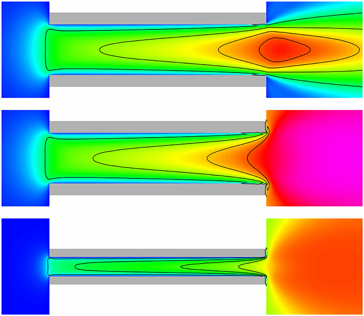
Figure 9. Set 1: PR with 100 SCCM of Ar, p₀ = 0.349 Torr (top); Set 3: PR with 100 SCCM of Ar (middle); Set 4: MiniPR with 60 SCCM of Xe (bottom). The color map and isocurves use the same scale as in Figure 6.

On the other hand, the flow is slightly slower in the Set 1 case. As such, the sonic surface is not developed to the full extent within the discharge volume, leaving only a supersonic flow area for r ≤ 0.73 mm. Hence, the flow in the Set 1 case is only partially choked. For Set 1, this behavior only manifests at flow rates beyond about 75 SCCM. Below this value, the flow velocity in PR is completely subsonic. This shows that the 4 : 1 pressure ratio, although being higher than the critical pressure ratio given by Equation (4), is still insufficient for choked flow to occur. This further reinforces that Equation (4) cannot be used in cases where the pressure drop is not immediate.

5.5. Thrust

The thrust from cold gas or electrothermal thrusters is derived from the momentum of the exhausted neutral gas propellant, as distinct from electrostatic or electromagnetic thrusters, where the thrust is defined as the force in reaction to the acceleration of ions through an electric field [71, 72]. PR belongs to the former class of neutral gas thrusters; it operates as an electrothermal microthruster when RF power is supplied to ionize and heat the neutral gas propellant [30, 31], and as a cold gas microthruster when no RF power is supplied.

The general thrust equation is used to calculate the thrust generated by neutral gas thrusters, including conventional rockets:

$\begin{array}{ll}{F}_{\mathrm{\text{t}}}=ṁ\left(u_{z,\mathrm{\text{e}}}-u_{z,\mathrm{\text{0}}}\right)+\left(p_{\mathrm{\text{e}}}-p_0\right)A_{\mathrm{\text{e}}}& (5)\end{array}$

where ṁ is the mass flow rate of the gas, A is the area, and the subscripts “e” and “0” denote exit and the ambient free stream respectively. For the present purpose, the free stream velocity u_{z, 0} is zero, and the free stream pressure is defined to be equal to the outlet pressure. The first term in Equation (5) represents the component of the thrust force arising from the momentum of the ejected propellant, while the second term represents the pressure force difference between the exit area and the equivalent area on the (external) front of PR.

In cases where p_e ≈ p₀ and u_{z, e} ≈ c_s across the exit, the equation ${\tilde{F}}_T=ṁc_{\mathrm{\text{s}}}$ may be used to give a rough estimation of the thrust. For high pressure and large geometries as in conventional rocket nozzles, this approximation is valid as the mass density, axial velocity, and pressure are typically uniform in the main flow across most of the exit area. However, for low pressure and small geometries like in microthrusters, boundary layer effects near the wall are nontrivial and often significant compared to the main flow, resulting in nonuniform profiles for all the three parameters. This is evident in PR, as shown in Figure 10, which displays the axial velocity (red), density (black), and pressure (blue) profiles across the exit for the 100 SCCM Ar simulation in Set 1 (solid lines) and Set 3 (dash-dotted lines). The profiles for the rest of the simulations of other flow rates are not shown as they are very similar in shape, with the only difference being the heights of the respective profiles.

FIGURE 10

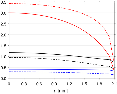
Figure 10. Radial profiles of the axial velocity (red, scale: × 10² m·s⁻¹), density (black, scale: × 10⁻³ kg·m⁻³), and pressure (blue, scale: Torr) at the exit z = 0 mm for the 100 SCCM Ar PR simulation in Set 1 (solid lines) and Set 3 (dash-dotted lines).

Additionally, as shown in Figure 9 for cylindrical geometries, the sonic surface is not planar and its position does not coincide with the exit surface, and can vary significantly depending on the gas and the choked flow conditions. Furthermore, the local sound speed c_s at the exit is dependent on the local temperature, which may be different from the initial temperature or stagnation temperature of the gas upstream, and difficult to measure. In cases where p_e ≠ p₀, and especially for space applications when p_e > p₀, the pressure thrust can be significant and its contribution must be taken into account with the addition of a term in the form of p_eA_e, though in practice p_e cannot be measured easily.

In these circumstances, calculation of the thrust requires the integral form of the general thrust equation:

$\begin{array}{ll}{F}_{\mathrm{\text{t}}}=2\pi {\displaystyle {\int }_0^R}r\left({\rho }_{\mathrm{\text{e}}}{u}_{z,\mathrm{\text{e}}}^2+p_{\mathrm{\text{e}}}-p_0\right)\mathrm{\text{d}}r& (6)\end{array}$

with the radial density ρ_e, axial velocity u_{z, e}, and pressure p_e profiles across the exit, integrated from the axis at r = 0 mm to the wall at r = 2.1 mm.

To ascertain the accuracy of the thrust calculations, a similar integration of the mass flow rate of the gas is performed across the exit area. It is found that the flow rate across the exit to be consistently 2.8–2.2% below the range of set values (for ascending flow rates) in Set 1, and 4.9–4.1% in Set 3. In Set 3, the corresponding values are 1.5–0.4% for the p₀ = p_c cases and 3.4–2.7% for the p₀ = 0 Torr cases. This small error may be attributed to the use of only 21 cells across the radius of the exit, resulting in the trapezoidal underestimation of the concave down profiles, or the deficiencies of the CFD-ACE+ code in dealing with supersonic flows at Mach numbers higher than 2. Additionally, because the axial velocity at the wall is not zero due to the fictitious slip velocity imposed by the slip boundary conditions, the thrust contribution from the boundary layer will be very slightly overestimated. However, while this uncertainty is not quantifiable, it should be negligible compared to the mass flow rate error. Consequently, it is likely that the thrust calculation underestimates the real thrust by the aforementioned amounts.

Figure 11 plots the calculated raw thrust values for the Set 1 and Set 3 simulations using 25–144 SCCM of Ar. The thrust for the Set 1 simulations is 47–38% less (for ascending flow rates) than the Set 3 simulations primarily due to the much larger pressure thrust arising from the large difference between the exit pressure p_e and the ambient pressure p₀ = 0 Torr, which accounts for 48–32% of the total thrust in Set 3. In Set 1, particularly for higher flow rates, the exit pressure is very close to the ambient pressure, therefore the pressure thrust is very small, and mass thrust accounts for almost all of the total thrust (65% for 25 SCCM, 82–92% for 50–144 SCCM).

FIGURE 11

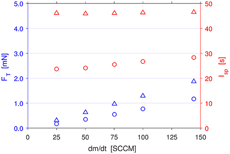
Figure 11. Calculated thrust (blue) and specific impulse (red) for PR simulations in Set 1 (circles) and Set 3 (triangles). Thrust increases linearly with flow rate, while specific impulse remains roughly constant. The specific impulse for Set 3 is close to the theoretical maximum value of 57.0 s for Ar.

For comparison, the calculated raw thrust values for the Set 2 PR nozzle simulations are plotted in Figure 12. The p₀ = 0 Torr cases in Set 2 perform only 1.3–6.6% better than the simulations in Set 3. On the other hand, the p₀ = p_c cases in Set 2 perform 2.9–12.6% better than the Set 1 simulations for flow rates 50–144 SCCM, but sees a 6.6% decrease in performance for the 25 SCCM simulation. This decrease in thrust for the 25 SCCM simulation in Set 2 is due the premature deceleration of the flow while it is still inside the divergent section of the nozzle by the static gas present in the downstream region. For the p₀ = 0 Torr cases, the flow at the exit is slightly less underexpanded than in Set 3, meaning that the pressure thrust is less dominant, accounting for 38–17% of the total thrust. For the p₀ = p_c cases however, the flow at the exit is overexpanded for flow rates above 50 SCCM, meaning that the pressure thrust is negative, and detracts from the total thrust.

FIGURE 12

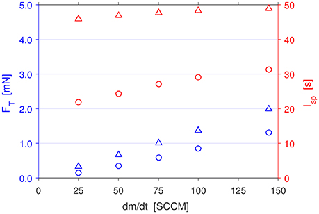
Figure 12. Calculated thrust (blue) and specific impulse (red) for PR converging-diverging nozzle simulations in Set 2: laboratory condition (circles) and vacuum condition (triangles). Thrust increases linearly with flow rate, with a slightly higher gradient compared to Set 1 and Set 3. The specific impulse for Set 2 vacuum condition is higher than Set 3, and close to the theoretical maximum value of 57.0 s for Ar.

Overall, there is not a large difference between the performance of the PR nozzle model and the original PR model mainly due to the fact that the present design of the nozzle is not optimized for either vacuum or any pressure in particular. However, this comparison serves to demonstrate that the generated amount of thrust is ultimately determined by the mass flow rate of the propellant rather than the stagnation pressure, as the Set 2 simulations generate only marginally higher thrust even though they have about twice the stagnation pressures of their counterparts in Set 1 and Set 3 for the same flow rates.

5.6. Specific Impulse

The specific impulse is a measure of the efficiency of a thruster, defined as the change in momentum delivered per unit of propellant. For neutral gas thrusters, the theoretical maximum specific impulse a gas can achieve is given by the following thermodynamic relation:

$\begin{array}{ll}{\overline{I}}_{\text{sp}}=\frac{1}{g}\cdot {\left\{\frac{k_{\text{B}}{T}_{\text{s}}}{m}·\frac{2\gamma }{\gamma -1}·\left[1-{\left(\frac{p_0}{p_{\text{s}}}\right)}^{\frac{\gamma -1}{\gamma }}\right]\right\}}^{\frac{1}{2}}& (7)\end{array}$

where g = 9.81 m·s⁻² is the standard acceleration due to gravity, $k_{\mathrm{\text{B}}}=1.38064852\times 10^{-23}\mathrm{\text{J}}·{\mathrm{\text{K}}}^{-1}$ is the Boltzmann constant, γ is the adiabatic index, m is the atomic mass of the gas, and T_s and p_s represent the stagnation temperature and pressure respectively. The p₀ term within the parentheses assumes that the flow at the exit is perfectly expanded such that p_e = p₀. For expansion into vacuum, Ī_sp becomes independent of p_s, and is solely determined by T_s. For T_s = 300 K, the theoretical maximum specific impulse for monatomic Ar gas is 57.0 s.

Figures 11, 12 plots the specific impulse of all the preceding simulations, calculated via dividing Equation (6) by the integrated mass flow rate across the exit area of the respective simulations. Overall, the Ī_sp is approximately constant across the range of flow rates, as expected from theory. There is some deviation from the constant value in the Set 3 simulations as seen in Figure 12, indicating that the converging-diverging nozzle is more efficient at higher flow rates.

To obtain the maximum possible total thrust, an optimized nozzle should be used to expand the exhaust such that p_e = p₀, and all of the thrust is derived from the momentum of the ejected propellant. While this is easily achieved in a pressurized environment even with just a cylindrical tube as shown in the Set 1 simulations, it is in practice impossible to achieve in vacuum as it would require an infinitely long nozzle. Despite that fact, the lower downstream pressure of the Set 3 simulations allow the propellant to be accelerated to a higher axial velocity across more of the exit area, resulting in an average specific impulse that is considerably closer to the theoretical maximum value.

Using the 100 SCCM Ar case for comparison, the calculated specific impulse and the relative percentage to the theoretical maximum value are as follows: Set 1: 26.8 s (72.4% of Ī_sp); Set 3: 46.4 s (81.4% of Ī_sp); Set 2, p₀ = 0.349 Torr: 29.1 s (68.0% of Ī_sp); and finally Set 2, p₀ = 0 Torr: 48.3 s (84.8% of Ī_sp). Note that Ī_sp is calculated with the respective p₀ and p_s values of each simulation. From these values, it can be concluded that the converging-diverging nozzle is more efficient than the cylindrical geometry for expansion into a vacuum environment. In a pressurized environment however, the unoptimized nozzle will overexpand the flow, resulting in a lower efficiency than the underexpanded flow in the cylindrical geometry case.

5.7. Boundary Layer Friction Force

Figure 13 shows two equivalent methods for calculating thrust, using the geometry of PR as an example. The general thrust equation involves summing all the forces acting upon the volume of gas from the exterior, while the internal forces method involves summing all the forces acting upon the surroundings from within the interior of the gas. As mentioned previously, the general thrust Equation (5) takes into account both the force from the momentum of the ejected propellant and the pressure force difference between the external front and rear faces of the microthruster.

FIGURE 13

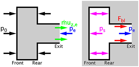
Figure 13. Force diagrams for the general thrust equation (left) and the internal forces method (right), where ṁu_{z, e} represents the force from the ejected propellant at the exit, p₀ is the ambient pressure, p_e is the exit pressure, p_s is the stagnation pressure in the plenum, and F_bl is the boundary layer friction force acting upon the wall of the discharge volume.

On the other hand, when using the alternative internal forces method, the total thrust is given by:

$\begin{array}{ll}{F}_{\mathrm{\text{t}}}=\left(p_{\mathrm{\text{s}}}-p_{\mathrm{\text{e}}}\right)A_{\mathrm{\text{e}}}-F_{\mathrm{\text{bl}}}& (8)\end{array}$

where p_s is the stagnation pressure of the gas in the plenum, and F_bl is the friction force between the boundary layer and the wall. To explain the origin of F_bl, suppose an inviscid fluid was used with a frictionless, adiabatic wall. Then the axial velocity of the flow would be high and uniform across the diameter and length of the discharge volume, and p_s in the plenum would be low as the gas is able to exit without any resistance. In this hypothetical case, since F_bl = 0, the total thrust is just the force difference between the internal front and rear faces given by (p_s − p_e)A_e.

Suppose the flowing fluid was then imbued with the viscosity and friction (represented by α_u) of a real gas. Then the gas molecules incident on the wall must slow down due to the friction, and the axial velocity of the surrounding flow would also decrease due to the viscosity of the fluid. This produces a velocity profile that is peaked in the middle of the discharge volume, as expected with laminar pipe flow in the continuum and slip regimes. The deceleration of the boundary layer flow compared to the main flow is evidence that momentum is being transferred from the flow to the wall through friction and viscosity effects, resulting in a force F_bl acting in the direction of flow. Since this direction is opposite to the direction of intended motion, F_bl detracts from the total thrust.

As a direct consequence of F_bl, p_s in the plenum would increase as the flow through the discharge volume becomes restricted by the boundary layer effects. Additionally, if the wall were nonadiabatic, the wall material would act as a thermal source (or sink), and further increase (or decrease) p_s accordingly. For flows on larger scales or where Kn → 0, p_s remains mostly unaffected and the magnitude of F_bl is negligible when compared with the net pressure force term in Equation (8). However, on miniature scales as in PR, p_s is greatly inflated and F_bl manifests as an unavoidable and significant fraction of the inflated net pressure force. Hence, using the inflated p_s without accounting for F_bl will result in a overestimation of the total thrust.

In practice, F_bl by itself is difficult to quantify. Nevertheless, F_bl can be calculated by equating Equations (5) and (8) when all the other variables are known. Since F_bl is dependent on the location and extensiveness of the boundary layer, it is ultimately dependent on the geometry of the microthruster. In the case of the original PR geometry used in Set 1 and Set 3, F_bl is 0.56–1.46 mN (for ascending flow rates), acting upon the wall of the discharge volume. As for the converging-diverging nozzle PR geometry used in Set 2, F_bl mostly acts upon the wall of the divergent section of the nozzle, where the velocity of the main flow relative to the wall is the highest, with the component in the axial direction (as opposed to parallel with the wall) being 1.24–5.04 mN.

These values show that F_bl can be, and is in fact often higher than the total thrust generated by PR. This is clear evidence that boundary layer effects are significant and must be accounted for, and calculations which are usually used for conventional rockets cannot be used for microthrusters operating at low pressure and with dimensions similar to or smaller than PR. Despite its inconvenience, information on the magnitude of F_bl can be used to optimize the surface properties or geometry of the microthruster, and thereby maximize thrust.

5.8. Set 4: MiniPR Vacuum Condition

To validate the CFD simulation and thrust calculation results, a fourth set of simulations is performed using the MiniPR mesh to compare with published experimental results of MiniPR in the Wombat space simulation chamber [27]. The chamber pressure was under 1 mTorr with full gas flow; having verified that the simulation results are insensitive to the outlet pressure at this pressure range, the outlet pressure was set at p₀ = 0 Torr for each case with 15–60 SCCM of Xe.

Using α_u = 1.0 for Xe [38, 44], the simulated plenum pressures obtained across the range of flow rates closely match the experimentally measured values, with a small systematic discrepancy of about +0.28 Torr, or equivalent to −2.3 SCCM attributed to the miscalibration of the mass flow controller if the pressure measurements are taken to be the baseline. This error is reasonable as the mass flow controller in the experiment was calibrated for Xe by measuring the volume displacement of the gas in water. Following the same data analysis procedure as above, it is found that the mass flow rate error at the exit is 10.8–10.1% under the set values, somewhat higher than the PR simulations due to the MiniPR mesh only having 8 cells across the radius of the exit.

As MiniPR has the same cylindrical geometry as PR, the flow behavior is very similar to that shown in Figures 4, 5. For reference, Figure 9 includes an illustration of the flow conditions in MiniPR (bottom). Note that the sound speed in Xe is lower than in Ar, so the flow velocities in MiniPR is lower than in PR. Since the sonic surface is determined by geometry, the sonic surface in MiniPR has the same parabolic shape as that in PR.

The cold gas thrust for MiniPR is calculated as before, with the axial velocity, density, and pressure profiles across the exit (red, black, and blue dash-dotted lines) plotted in Figure 14. Figure 15 plots the calculated thrust (blue triangles) along with the experimental results (magenta squares) from Charles et al. [27]. In the experiment, the cold gas thrust was measured after the gas flow had been shut off at the mass flow controller. This means that the gas entering MiniPR was from the residual volume of gas trapped in the gas line (d = 1 mm, l = 4 m) between the mass flow controller and MiniPR. As the trapped gas require many hours to be fully depleted, it is reasonable to approximate a constant but slightly diminished flow rate in the short duration when each measurement was taken. Assuming a 30% decrease in the flow rate after the flow was turned off, the corrected cold gas thrust values (green squares) become in line with the simulated thrust values. Since MiniPR has the same geometry as PR, p_e will not be expanded to zero. Thus, the pressure thrust is significant and accounts for 33–27% of the total thrust for ascending flow rates of Xe. For comparison, F_bl in MiniPR is 0.55–1.04 mN.

FIGURE 14

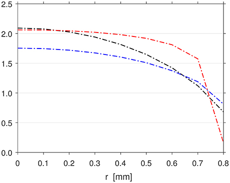
Figure 14. Radial profiles of the axial velocity (red dash-dotted line, scale: × 10² m·s⁻¹), density (black dash-dotted line, scale: × 10⁻² kg·m⁻³), and pressure (blue dash-dotted line, scale: Torr) at the exit z = 0 mm for the 60 SCCM Xe MiniPR simulation in Set 4, representative of the experiment in Charles et al. [27].

FIGURE 15

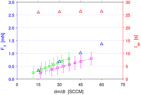
Figure 15. Calculated thrust (blue) and specific impulse (red) for Set 4 MiniPR simulations (triangles), along with the experimentally measured thrust from Charles et al. [27] (magenta squares) and their corrected values (green squares). The specific impulse for Set 4 is close to the theoretical maximum value of 31.4 s for Xe.

The theoretical maximum specific impulse of Xe is 31.4 s for T_s = 300 K. The average I_sp calculated from the MiniPR Xe simulations is 26.2 s (83.4% of Ī_sp), showing a relative performance consistent with the Set 3 PR simulations using Ar. The lower cold gas I_sp reported in Charles et al. [27] is unlikely to be due to a lower T_s as MiniPR was in thermal contact with the surrounding environment through the thrust balance. Operating with a plasma raises the effective T_s, which increases the thrust and I_sp performance; the highest I_sp was obtained at the lowest flow rate, as a smaller mass of propellant is able to reach higher temperatures when a constant amount of power was applied [27].

In the current cylindrical geometry of PR and MiniPR, the experimentally measured I_sp cannot be used to accurately estimate the temperature of the plasma-heated gas in the discharge volume since the gas is not stagnant but moving at a significant fraction of the local c_s where the heating occurs. The implementation of a converging-diverging nozzle will allow a better estimation of T_s and the real gas temperature in the region upstream of the throat where the axial velocity of the gas is slow. Apart from the advantage of being able to generate more thrust from the expansion of the exhaust propellant in the nozzle, the longer transit time through the discharge volume will result in more effective gas heating, and bring about higher thrust and I_sp performance.

6. Conclusion

In summary, cold gas simulations of PR and MiniPR with multiple gases have been performed using CFD-ACE+ to construct flow models to complement and compare with cold gas experimental measurements of the PR and MiniPR microthrusters. This work demonstrates that using a slip boundary condition with the correct tangential momentum accommodation coefficient results in precise agreement with the experimentally measured plenum pressure and realistic flow behavior. The upstream behavior of the expansion of gas from PR and MiniPR into vacuum can be accurately modeled even with a fluid solver, provided that the simulation program is able to treat flow velocity choking. The thrust was calculated by integrating the flow profiles at the exit, and the uncertainty was deduced by evaluating the discrepancy between the set mass flow rate and the integrated mass flow rate at the exit. The simulated thrust is verified to be reasonable as the calculated specific impulse of each simulation is very close to the theoretical maximum value. Finally, the simulation results for thrust and the plenum stagnation pressure are validated by comparing them to experimentation results, and are found to be in good agreement.

The concurrence of the simulated specific impulse to the theoretical maximum values as well as the good agreement with the experimental measurements indicate that the simulations produce sound and reliable models for the cold gas operations of both PR and MiniPR. For low thrust conditions where experimental instruments are not sufficiently sensitive, cold gas simulations can provide additional data points against which experimental results could be verified and extrapolated. The cold gas simulations presented in this paper will be used as a benchmark to compare with future plasma simulations of PR also performed in CFD-ACE+.

Author Contributions

CC and RB devised the project and designed the basic structure of the research. They both supervised TSH, their Ph.D. student.

Funding

This research was funded by the Australian Research Council Discovery Project DP140100571, by the Australian Space Research Program [Wombat upgrade as part of the Australian Plasma Thruster (APT) project] of the Department of Industry, Innovation, Science, Research and Tertiary Education (Australian Government), and Lockheed Martin US (Pocket Rocket thruster Research and Development contract).

Conflict of Interest Statement

The authors declare that the research was conducted in the absence of any commercial or financial relationships that could be construed as a potential conflict of interest.

References

1. Gill E, Sundaramoorthy P, Bouwmeester J, Zandbergen B, Reinhard R. Formation flying within a constellation of nano-satellites: the QB50 mission. Acta Astronaut. (2012) 82:110–7. doi: 10.1016/j.actaastro.2012.04.029

CrossRef Full Text | Google Scholar

2. Virgili J, Roberts PCE. ΔDsat, a QB50 CubeSat mission to study rarefied-gas drag modelling. Acta Astronaut. (2013) 89:130–8. doi: 10.1016/j.actaastro.2013.04.006

CrossRef Full Text | Google Scholar

3. Hitt DL, Zakrzwski CM, Thomas MA. MEMS-based satellitemicropropulsion via catalyzed hydrogen peroxide decomposition. Smart Mater Struct. (2001) 10:1163–75. doi: 10.1088/0964-1726/10/6/305

CrossRef Full Text | Google Scholar

4. Horisawa H, Kimura I. Very low-power arcjet testing. Vacuum (2000) 59:106–17. doi: 10.1016/S0042-207X(00)00260-8

CrossRef Full Text | Google Scholar

5. Horisawa H, Ashiya H, Kimura I. Discharge characteristics of a very low-power arcjet. In: International Electric Propulsion Conference. Toulouse (2003). p. 1–8.

6. Böhrk H, Auweter-Kurtz M. Thrust measurement of the hybrid electric thruster TIHTUS by a baffle plate. J Propul Power (2009) 25:729–36. doi: 10.2514/1.34324

CrossRef Full Text | Google Scholar

7. Ketsdever AD, Lee RH, Lilly TC. Performance testing of a microfabricated propulsion system for nanosatellite applications. J Micromech Microeng. (2005) 15:2254–63. doi: 10.1088/0960-1317/15/12/007

CrossRef Full Text | Google Scholar

8. Lamprou DA, Lappas VJ, Shimizu T, Gibbon D, Perren M. Hollow cathode thruster design and development for small satellites. In: International Electric Propulsion Conference. Wiesbaden (2011). p. 1–10.

Google Scholar

9. Grubisic AN, Gabriel SB. Assessment of the T5 and T6 hollow cathodes as reaction control thrusters. J Propul Power (2016) 32:810–20. doi: 10.2514/1.B35556

CrossRef Full Text | Google Scholar

10. Charles C, Boswell RW. Measurement and modelling of a radiofrequency micro-thruster. Plasma Sour Sci Technol. (2012) 21:1–4. doi: 10.1088/0963-0252/21/2/022002

CrossRef Full Text | Google Scholar

11. Patterson MJ, Foster JE, Young JA, Crofton MW. Annular engine development status. In: Joint Propulsion Conference. San Jose, CA: American Institute of Aeronautics and Astronautics (2013). p. 1–18. doi: 10.2514/6.2013-3892

CrossRef Full Text | Google Scholar

12. Patterson MJ, Thomas R, Crofton MW, Young JA, Foster JE. High thrust-to-power annular engine technology. In: Joint Propulsion Conference. Orlando, FL: American Institute of Aeronautics and Astronautics (2015). p. 1–16. doi: 10.2514/6.2015-3719

CrossRef Full Text | Google Scholar

13. Patterson M, Benson S. NEXT ion propulsion system development status and performance. In: Joint Propulsion Conference. Cincinnati, OH: American Institute of Aeronautics and Astronautics (2007). p. 1–17. doi: 10.2514/6.2007-5199

CrossRef Full Text | Google Scholar

14. Polk JE, Kamhawi H, Polzin K, Brophy JR, Ziemer J, Smith TD, et al. An overview of NASA's electric propulsion programs, 2010–11. In: International Electric Propulsion Conference. Wiesbaden (2011). p. 1–28.

15. Gonzalez J, Saccoccia G, von Rhoden H. Field emission electric propulsion: experimental investigations on microthrust FEEP thrusters. In: International Electric Propulsion Conference. Seattle, WA (1993). p. 1–9.

16. Goebel DM, Katz I. Fundamentals of Electric Propulsion. Ion and Hall Thrusters. Hoboken, NJ: Wiley (2008). doi: 10.1002/9780470436448

CrossRef Full Text | Google Scholar

17. Khayms V. Advanced Propulsion for Microsatellites. Cambridge, MA: Massachusetts Institute of Technology (2000).

Google Scholar

18. Hargus WA, Charles CS. Near exit plane velocity field of a 200-Watt Hall thruster. J Propul Power (2008) 24:127–33. doi: 10.2514/1.29949

CrossRef Full Text | Google Scholar

19. Hofer R. High-specific impulse operation of the BPT-4000 Hall thruster for NASA science missions. In: Joint Propulsion Conference. Nashville, TN: American Institute of Aeronautics and Astronautics (2010).

20. LaPointe MR, Mikellides PG. High power MPD thruster development at the NASA Glenn Research Center. In: Joint Propulsion Conference. Salt Lake City, UT: American Institute of Aeronautics and Astronautics (2001). p. 1–11.

21. Kodys AD, Choueiri EY. A critical review of the state-of-the-art in the performance of applied-field magnetoplasmadynamic thrusters. In: Joint Propulsion Conference. Tucson, AZ: American Institute of Aeronautics and Astronautics (2005). p. 1–23.

22. Keidar M, Zhuang T, Shashurin A, Teel G, Chiu D, Lukas J, et al. Electric propulsion for small satellites. Plasma Phys Control Fusion (2015) 57:1–10. doi: 10.1088/0741-3335/57/1/014005

CrossRef Full Text | Google Scholar

23. Charles C. Plasmas for spacecraft propulsion. J Phys D Appl Phys. (2009) 42:1–18. doi: 10.1088/0022-3727/42/16/163001

CrossRef Full Text

24. Mazouffre S. Electric propulsion for satellites and spacecraft: established technologies and novel approaches. Plasma Sources Sci Technol. (2016) 25:1–27. doi: 10.1088/0963-0252/25/3/033002

CrossRef Full Text | Google Scholar

25. Micci MM, Ketsdever AD. Micropropulsion for Small Spacecraft. Reston, VA: AIAA (2000).

Google Scholar

26. Scharfe D, Ketsdever AD. A review of high thrust, high delta-v options for microsatellite missions. In: Joint Propulsion Conference. Denver, CO (2009). p. 1–14.

Google Scholar

27. Charles C, Boswell RW, Bish A, Khayms V, Scholz EF. Direct measurement of axial momentum imparted by an electrothermal radiofrequency plasma micro-thruster. Front Phys. (2016) 4:19. doi: 10.3389/fphy.2016.00019

CrossRef Full Text | Google Scholar

28. Greig A. Pocket Rocket: An Electrothermal Plasma Micro-Thruster. Canberra: The Australian National University (2015).

Google Scholar

29. Charles C, Boswell RW, Takahashi K. Investigation of radiofrequency plasma sources for space travel. Plasma Phys Control Fusion (2012) 54:1–7. doi: 10.1088/0741-3335/54/12/124021

CrossRef Full Text | Google Scholar

30. Greig A, Charles C, Paulin N, Boswell RW. Volume and surface propellant heating in an electrothermal radio-frequency plasma micro-thruster. Appl Phys Lett. (2014) 105:1–4. doi: 10.1063/1.4892656

CrossRef Full Text | Google Scholar

31. Greig A, Charles C, Hawkins R, Boswell RW. Direct measurement of neutral gas heating in a radio-frequency electrothermal plasma micro-thruster. Appl Phys Lett. (2013) 103:1–4. doi: 10.1063/1.4818657

CrossRef Full Text | Google Scholar

32. Greig A, Charles C, Boswell RW. Spatiotemporal study of gas heating mechanisms in a radio-frequency electrothermal plasma micro-thruster. Front Phys. (2015) 3:84. doi: 10.3389/fphy.2015.00084

CrossRef Full Text | Google Scholar

33. Greig A, Charles C, Boswell RW. Neutral gas temperature estimates and metastable resonance energy transfer for argon-nitrogen discharges. Phys Plasmas (2016) 23:1–10. doi: 10.1063/1.4939028

CrossRef Full Text | Google Scholar

34. Charles C, Boswell RW, Bish A. Low-weight fixed ceramic capacitor impedance matching system for an electrothermal plasma microthruster. J Propul Power (2014) 30:1117–21. doi: 10.2514/1.B35119

CrossRef Full Text | Google Scholar

35. Charles C, Bish A, Boswell RW, Dedrick J, Greig A, Hawkins R, et al. A short review of experimental and computational diagnostics for radiofrequency plasma micro-thrusters. Plasma Chem Plasma Process. (2015) 36:29–44. doi: 10.1007/s11090-015-9654-5

CrossRef Full Text | Google Scholar

36. La Torre F. Gas Flow in Miniaturized Nozzles for Micro-Thrusters. Delft: Delft University of Technology (2011).

Google Scholar

37. Maxwell JC. On Stresses in rarified gases arising from inequalities of temperature. Philos Trans R Soc Lond. (1879) 170:231–56. doi: 10.1098/rstl.1879.0067

CrossRef Full Text | Google Scholar

38. Porodnov BT, Suetin PE, Borisov SF, Akinshin VD. Experimental investigation of rarefied gas flow in different channels. J Fluid Mech. (1974) 64:417–38. doi: 10.1017/S0022112074002485

CrossRef Full Text | Google Scholar

39. Arkilic EB, Breuer KS, Schmidt MA. Mass flow and tangential momentum accommodation in silicon micromachined channels. J Fluid Mech. (2001) 437:29–43. doi: 10.1017/S0022112001004128

CrossRef Full Text | Google Scholar

40. Maurer J, Tabeling P, Joseph P, Willaime H. Second-order slip laws in microchannels for helium and nitrogen. Phys Fluids (2003) 15:2613–21. doi: 10.1063/1.1599355

CrossRef Full Text | Google Scholar

41. Colin S, Lalonde P, Caen R. Validation of a second-order slip flow model in rectangular microchannels. Heat Transfer Eng. (2004) 25:23–30. doi: 10.1080/01457630490280047

CrossRef Full Text | Google Scholar

42. Ewart T, Perrier P, Graur IA, Méolans JG. Tangential momemtum accommodation in microtube. Microfluidics Nanofluidics (2007) 3:689–95. doi: 10.1007/s10404-007-0158-3

CrossRef Full Text | Google Scholar

43. Graur IA, Perrier P, Ghozlani W, Méolans JG. Measurements of tangential momentum accommodation coefficient for various gases in plane microchannel. Phys Fluids (2009) 21:1–9. doi: 10.1063/1.3253696

CrossRef Full Text | Google Scholar

44. Perrier P, Graur IA, Ewart T, Méolans JG. Mass flow rate measurements in microtubes: from hydrodynamic to near free molecular regime. Phys Fluids (2011) 23:1–11. doi: 10.1063/1.3562948

CrossRef Full Text | Google Scholar

45. Yamaguchi H, Hanawa T, Yamamoto O, Matsuda Y, Egami Y, Niimi T. Experimental measurement on tangential momentum accommodation coefficient in a single microtube. Microfluidics Nanofluidics (2011) 11:57–64. doi: 10.1007/s10404-011-0773-x

CrossRef Full Text | Google Scholar

46. Hadj Nacer M, Graur IA, Perrier P, Méolans JG, Wuest M. Gas flow through microtubes with different internal surface coatings. J Vacuum Sci Technol A Vacuum Surf Films (2013) 32:1–9. doi: 10.1116/1.4828955

CrossRef Full Text | Google Scholar

47. Smoluchowski von Smolan M. Ueber Wärmeleitung in verdünnten Gasen. Ann Phys. (1898) 300:101–30. doi: 10.1002/andp.18983000110

CrossRef Full Text | Google Scholar

48. Vargaftik NB, Voshchinin AA, Kerzhentsev VV. Experimental determination of the accommodation coefficients of argon and xenon on nickel at high temperatures. J Eng Phys. (1973) 25:1391–3. doi: 10.1007/BF00838115

CrossRef Full Text | Google Scholar

49. Porodnov BT, Kulev AN, Tuchvetov FT. Thermal transpiration in a circular capillary with a small temperature difference. J Fluid Mech. (1978) 88:609–22. doi: 10.1017/S002211207800230X

CrossRef Full Text | Google Scholar

50. Song S, Yovanovich MM. Contact interface gas heat transfer: a method of measuring thermal accommodation coefficient. In: International Conference on Electronics Packaging. San Diego, CA (1989). p. 925–36.

Google Scholar

51. Rader DJ, Castañeda JN, Torczynski JR, Grasser TW, Trott WM. Measurements of Thermal Accommodation Coefficients. Albuquerque, NM: Sandia National Laboratories, SAND2005-6084 (2005).

Google Scholar

52. Ganta D, Dale EB, Rezac JP, Rosenberger AT. Optical method for measuring thermal accommodation coefficients using a whispering-gallery microresonator. J Chem Phys. (2011) 135:1–7. doi: 10.1063/1.3631342

PubMed Abstract | CrossRef Full Text | Google Scholar

53. Trott WM, Castañeda JN, Torczynski JR, Gallis MA, Rader DJ. An experimental assembly for precise measurement of thermal accommodation coefficients. Rev Sci Instrum. (2011) 82:1–12. doi: 10.1063/1.3571269

PubMed Abstract | CrossRef Full Text | Google Scholar

54. Yamaguchi H, Kanazawa K, Matsuda Y, Niimi T, Polikarpov A, Graur IA. Investigation on heat transfer between two coaxial cylinders for measurement of thermal accommodation coefficient. Phys Fluids (2012) 24:1–16. doi: 10.1063/1.4726059

CrossRef Full Text | Google Scholar

55. Thomas LB, Olmer F. The accommodation coefficients of He, Ne, Ar, H₂, D₂, O₂, CO₂, and Hg on platinum as a function of temperature. J Am Chem Soc. (1943) 65:1036–43. doi: 10.1021/ja01246a011

CrossRef Full Text | Google Scholar

56. Kogan MN. Rarefied Gas Dynamics. New York, NY: Springer (1969).

57. Karniadakis GE, Beskok A, Aluru N. Microflows and Nanoflows. Fundamentals and Simulation. New York, NY: Springer (2005).

Google Scholar

58. Poling BE, Prausnitz JM, OConnell JP. The Properties of Gases and Liquids, 5th Edn. New York, NY: McGraw-Hill (2000).

Google Scholar

59. Lemmon EW, Friend DG. Thermophysical properties of fluid systems. In: Linstrom PJ, Mallard WG, editors. NIST Chemistry WebBook, NIST Standard Reference Database Number 69. National Institute of Standards and Technology.

60. Amdur I, Mason EA. Properties of gases at very high temperatures. Phys Fluids (1958) 1:370–83. doi: 10.1063/1.1724353

CrossRef Full Text | Google Scholar

61. Amdur I, Schatzki TF. Diffusion coefficients of the systems Xe-Xe and Ar-Xe. J Chem Phys. (1957) 27:1049–54. doi: 10.1063/1.1743930

CrossRef Full Text | Google Scholar

62. Dymond JH. High temperature transport coefficients for the rare gases neon to xenon. J Phys B (2001) 4:621–7. doi: 10.1088/0022-3700/4/4/025

CrossRef Full Text | Google Scholar

63. Hutchinson F. Self-diffusion in argon. J Chem Phys. (1949) 17:1081–6. doi: 10.1063/1.1747116

CrossRef Full Text | Google Scholar

64. Winn EB. The temperature dependence of the self-diffusion coefficients of argon, neon, nitrogen, oxygen, carbon dioxide, and methane. Phys Rev. (1950) 80:1024–7. doi: 10.1103/PhysRev.80.1024

CrossRef Full Text | Google Scholar

65. Winter ERS. Diffusion properties of gases. Part IV – the self-diffusion coefficients of nitrogen, oxygen, and carbon dioxide. Trans Faraday Soc. (1951) 47:342–7. doi: 10.1039/TF9514700342

CrossRef Full Text | Google Scholar

66. Cussler EL. Diffusion, 3rd Edn. Mass Transfer in Fluid Systems. Cambridge, MA: Cambridge University Press (2009).

67. Haynes WM. CRC Handbook of Chemistry and Physics, 96th Edn. Boca Raton, FL: CRC Press (2015).

68. MatWeb. Available online at: http://www.matweb.com/

69. Chapman CJ. High Speed Flow. Cambridge: Cambridge University Press (2000).

Google Scholar

70. Murphy HR, Miller DR. Effects of nozzle geometry on kinetics in free-jet expansions. J Phys Chem. (1984) 88:4474–8. doi: 10.1021/j150664a005

CrossRef Full Text | Google Scholar

71. Garrigues L, Hagelaar GJM, Bareilles J, Boniface C, Boeuf JP. Model study of the influence of the magnetic field configuration on the performance and lifetime of a Hall thruster. Phys Plasmas (2003) 10:4886–92. doi: 10.1063/1.1622670

CrossRef Full Text | Google Scholar

72. Garrigues L, Boniface C, Hagelaar GJM, Boeuf JP, Duchemin O. Performance modeling of a thrust vectoring device for Hall effect thrusters. J Propul Power (2009) 25:1003–12. doi: 10.2514/1.39680

CrossRef Full Text | Google Scholar