A Cell-Based Framework for Numerical Modeling of Electrical Conduction in Cardiac Tissue

1. Introduction

The pumping function of the heart is governed by an electrochemical wave traversing the entire cardiac muscle resulting in the muscle's synchronized contraction. This electrochemical wave has been subject to intense study over many decades and mathematical models have played an essential role in understanding its properties. However, these models are based on homogenization of the cardiac tissue, which imposes limitations on the level of detail that can be studied by the models. For instance, the details of the dynamics surrounding a single cell are difficult to study using classical homogenized models simply because the single cell is not present in such models.

In this paper, we consider an emerging mathematical modeling framework for representing and simulating excitable cells in general and cardiac cells in particular. In this framework, the extracellular space, the cell membranes, and the intracellular spaces are explicitly represented as separate physical and geometrical objects. The state variables are the extracellular, membrane, and intracellular potentials defined over the corresponding domains. We refer to this framework as the EMI (Extracellular-Membrane-Intracellular) model. This approach has been applied in several earlier papers (e.g., [1–7]), which used the EMI framework (or related approaches) for detailed simulations of a single cell or a small number of cells. Indeed, the presentation here is very much motivated by the formulation presented by Stinstra et al. [5] and by Agudelo-Toro and Neef [4]. Furthermore, the EMI approach was used to study the effect of the ephaptic coupling of neurons in Tveito et al. [8].

The EMI framework represents an alternative to the classical and more common bidomain or monodomain models. These latter models are based on homogenization of the cardiac tissue and the extracellular space, the intracellular space, and the cell membrane are all assumed to exist everywhere (e.g., [9–13]). In the following, when we refer to homogenized models, we will refer to models of the monodomain or bidomain type. In contrast, the EMI approach avoids this full homogenization at the tissue level. Note however, that homogenization is also used in the EMI approach to formulate equations for the intracellular domain and the extracellular domain.

The classical models (monodomain, bidomain) have been successfully used to study the propagation of the electrochemical wave in cardiac tissue (e.g., [14–16]), the initiation of excitation waves (e.g., [17–21]), the development of cardiac arrhythmias (e.g., [14, 17, 18]), the effect of defibrillation (e.g., [22–28]), and the effect of various drugs (e.g., [29–32]).

Despite the many successful applications of the monodomain and bidomain models, there are a number of motivating factors for introducing a more explicit, more accurate, and more detailed framework for modeling cardiac tissue. We address some of these factors in the following paragraphs.

1.1. Homogenized Models May Be Insufficient to Represent Details of the Remodeling of the Heart

Although, classical models represent the big picture of the electrochemical wave traversing cardiac tissue well, they may fail to reveal the finer details of cardiac conduction. For example, it is well-established that local perturbations to the conduction velocity may be arrhythmogenic; in particular, slowed conduction will increase the risk of arrhythmias [33]. It is therefore essential to understand how various remodelings of the heart affect the conduction velocity. Individual perturbations of the size and shape of the cardiac cells clearly affect the conduction velocity (e.g., [34]), but such changes are very hard to represent in a classical homogenized model, since a detailed representation of the individual cells in the tissue is needed. Furthermore, local density distributions of ion channels on the cell membrane will affect local conduction properties and such effects are also very hard, if even possible, to represent in the classical models.

1.2. Homogenized Models Are Unsuitable for Addressing the Ephaptic Coupling of Cardiac Cells

The electrical conduction of the heart is believed to depend on direct cell-to-cell contact realized in terms of gap junctions (e.g., [35–37]). These connections are reduced under heart failure, resulting in impaired conduction velocity that may in turn increase the probability of arrhythmias (e.g., [38, 37]). However, even when conduction through gap junctions is significantly reduced, electrical signals are still conducted (e.g., [39]). This conduction is believed to rely on ephaptic coupling between neighboring cells via the extracellular space. The effect depends on the shape and size of the extracellular space and is thus not directly amenable to analysis via the homogenized bidomain or monodomain models.

1.3. Simulating Cell Monolayers is of Increasing Significance

The number of cardiomyocytes in the human ventricles can be estimated to be around 8 billion (e.g., [40]), and the number is close to 4 million for the mouse heart (e.g., [41]). In both cases, a homogenized model may be justified by the large number of cells involved. However, for experimental setups with monolayers of cardiac cells, the number of cells is much lower (hundreds or a few thousands) and the validity of the homogenized continuum approach becomes questionable. The EMI model, on the other hand, is very well suited, since it represents every individual cell. The ability to faithfully simulate monolayers of cardiac cells has become very important since it has become possible to simultaneously measure the transmembrane potential and the intracellular calcium concentration (e.g., [42]). Therefore, at least in principle, the inversion of spatial models of monolayers may be applied to characterize properties of single cells using monolayer experiments. This is particularly important because of the development of human induced pluripotent stem cells (hi-PSC). Based on skin samples, such cells can be used to derive cardiac cells with certain properties identical to a patient's cardiac cells. Therefore, this technology is believed to have great potential in the development of personalized drugs for rare diseases (e.g., [43–45]).

1.4. Available Computational Power Allows for Cell Size Resolution

Twenty-five years ago, the best mathematical model of cardiac tissue was solved using 257 computational nodes [12, 46]. At that time, an accurate representation of cardiac tissue in terms of the representation of individual cells was inconceivable for reasons of both storage and computing time. This has changed dramatically; in recent computational studies, 29 million computational nodes were used to represent cardiac tissue [27, 47]. The computational mesh size in these simulations was about 59 μm, which should be compared with 100 μm, the typical length of a cardiac cell. This means that current simulators of the electrophysiology of the heart are, at least in principle, able to resolve features at the individual cell level.

The main purpose of the present paper is to assess the computational challenges of the EMI modeling framework. We will show how the model's complexity increases as the number of cardiac cells in the simulations increases and how the complexity of the membrane model affects the overall CPU demands.Furthermore, we will demonstrate that the EMI framework opens the possibility of simulating local properties of the cell that are hard to represent in homogenized models.

We introduce an operator splitting scheme for the EMI model and propose and compare three numerical schemes for the discretization of the resulting partial differential equations (PDEs): one finite difference-based (FDM) and two finite element-based (FEM) schemes of various degrees of complexity, computational cost, and accuracy. We compare the three schemes numerically in terms of convergence rates and computational cost. Moreover, to illustrate the distinctive capabilities of the EMI model, we present new results for simulating monolayers of cardiac cells with spatially heterogeneous distributions of ionic channels across the cell membrane.

Our results demonstrate that the EMI approach is computationally feasible: We can solve systems relevant for simulating monolayers of cardiac cells with sufficient resolution. Moreover, we show, using numerical computations based on the FDM code, that the computational effort per cell is bounded independently of the number of cardiac cells, and thus that the effort increases at most linearly with the number of cells.

1.5. Outline

In the next section, we will present the EMI model and three numerical methods used to solve the model. Next, we will discuss the numerical accuracy of the solutions, show convergence under mesh refinements, and assess the methods' CPU demands. To illustrate the ability to model local properties of individual cells, we present an example showing the difference in the conduction velocity of cells with uniform and non-uniform distributions of sodium channels. In the final sections, the results will be summarized and discussed.

2. Models and Methods

In this section, we present the EMI model and numerical methods for solving the corresponding set of equations.

2.1. The EMI Model

We will use the EMI model to simulate collections of cardiac cells. However, to present the model, it is sufficient to consider the case of two coupled cells.

We assume that the complete computational domain consists of intracellular spaces ${\Omega }_i^k$, with k = 1, 2 in the case of two cells, that are connected by gap junctions Γ_1,2 and surrounded by a connected extracellular space Ω_e. The membrane is defined to be the intersection between each intracellular domain ${\Omega }_i^k$ and the extracellular domain and is denoted by Γ_k, while the remaining boundary of the extracellular domain is denoted by ∂Ω_e. Figure 1 illustrates a two-dimensional (2D) version of this setup, showing two connected cells surrounded by extracellular space. In our computations (except in the first simple test case with an analytical solution) all cells are 3D and the cells can be connected in one-, two-, or three-dimensional collections. In one-dimensional strands of cells, the cell coupling is as illustrated in Figure 1; for two and three-dimensional collections of cells, the coupling in the y- and z-directions are similar to the x-coupling illustrated in the figure.

FIGURE 1

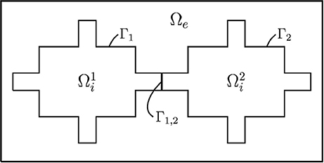
Figure 1. Illustration of an idealized computational domain: two idealized cells ${\Omega }_i^1$ and ${\Omega }_i^2$ connected by a gap junction Γ_1,2 and the surrounding extracellular domain Ω_e.

For the case illustrated in Figure 1, the EMI model can be formulated as follows: Find the extracellular potential u_e defined over Ω_e, the intracellular potentials $u_i^k$ defined over ${\Omega }_i^k$, and the transmembrane potentials v^k defined over Γ_k for k = 1, 2 and w defined over Γ_1,2 satisfying

$\begin{array}{ll}\nabla ·{\sigma }_e\nabla u_e=0\text{ in }{\Omega }_e,& (1)\end{array}$

$\begin{array}{ll}\nabla ·{\sigma }_i\nabla u_i^k=0\text{ in }{\Omega }_i^k,& (2)\end{array}$

$\begin{array}{ll}{u}_e=0\text{ at }\partial {\Omega }_e,& (3)\end{array}$

$\begin{array}{ll}{n}_e·{\sigma }_e\nabla u_e=-n_i^k·{\sigma }_i\nabla u_i^k\equiv I_m^k\text{ at }{\Gamma }_k,& (4)\end{array}$

$\begin{array}{ll}{u}_i^k-u_e=v^k\text{ at }{\Gamma }_k,& (5)\end{array}$

$\begin{array}{ll}{v}_t^k=\frac{1}{C_m}(I_m^k-I_{\text{ion}}^k)\text{ at }{\Gamma }_k,& (6)\end{array}$

$\begin{array}{ll}{n}_i^2·{\sigma }_i\nabla u_i^2=-n_i^1·{\sigma }_i\nabla u_i^1\equiv I_{1,2}\text{ at }{\Gamma }_{1,2},& (7)\end{array}$

$\begin{array}{ll}{u}_i^1-u_i^2=w\text{ at }{\Gamma }_{1,2},& (8)\end{array}$

$\begin{array}{ll}{w}_t=\frac{1}{C_{1,2}}(I_{1,2}-I_{\text{gap}})\text{ at }{\Gamma }_{1,2},& (9)\end{array}$

for k = 1, 2. Here, n_e is the normal pointing out from Ω_e and $n_i^k$ is the (outward) normal pointing out from ${\Omega }_i^k$ for k = 1, 2; σ_i and σ_e are the intracellular and extracellular conductivities, respectively; $I_{\text{ion}}^k$ represents the ionic current density, which typically depends on additional state variables such as ionic concentrations; and I_gap represents the gap junction current density. In terms of units, the potentials u_e, $u_i^k$, v^k, and w are given in mV; the current densities $I_m^k$, $I_{\text{ion}}^k$, I_1,2, and I_gap are given in μA/cm²; the conductivities σ_i and σ_e are given in mS/cm; the capacitances C_m and C_1,2 are given in μF/cm²; length is given in cm; and time is given in ms. In the following, we will refer to (1–9) as the EMI model. For brevity, we will write u_i in place of $u_i^k$, v in place of v^k, I_ion in place of $I_{\text{ion}}^k$ and Γ in place of Γ_k for k = 1, 2 when context allows.

2.2. Membrane Model

In our computations, we will consider both a passive and an active model for the dynamics on the cell membrane between the intracellular and extracellular spaces. In the passive model, I_ion is given by the linear model

$\begin{array}{ll}{I}_{\mathrm{\text{ion}}}(v)=\frac{1}{R_m}(v-v_{\mathrm{\text{rest}}}),& (10)\end{array}$

where R_m represents the resistance of the passive membrane (in kΩcm²) and v_rest denotes the resting potential of the membrane. In the active model, we let I_ion be represented by the action potential (AP) model of Grandi et al. [48]. In this case, Equation (6) is replaced by a system of the form

$\begin{array}{ll}{v}_t=\frac{1}{C_m}(I_m-I_{\text{ion}}(v,s)),& (11)\end{array}$

$\begin{array}{ll}{s}_t=F(v,s),& (12)\end{array}$

where v represents the membrane potential and s represents a collection of additional state variables introduced in the AP model. Furthermore, I_ion represents the sum of the ionic current densities across the membrane through a number of different types of ion channels, pumps, and exchangers and F(v, s) represents the ordinary differential equations (ODEs) describing the dynamics of the additional state variables. The Grandi model is implemented by defining a membrane potential v and a set of state variables s for each of the membrane nodes of the mesh. We let all state variables of the Grandi model, including the intracellular ionic concentrations, be defined only on the mesh nodes located on the cell membrane, and we allow the value of these variables to vary for different membrane nodes located on the same cell. The values of the state variables are updated in each time step using an operator splitting scheme described below. Intracellular and extracellular gradients of the ionic concentrations are ignored (see comment in section 4).

Finally, we represent the gap junction between neighboring cells by a passive membrane:

$\begin{array}{ll}{I}_{\mathrm{\text{gap}}}(w)=\frac{1}{R_{\text{gap}}}w,& (13)\end{array}$

where R_gap represents the resistance of the passive membrane (in kΩcm²). A discussion of the modeling of the gap-junctions is given in Hogues et al. [1] where a boundary element method is used to solve a model similar to the system (1–9).

2.3. Operator Splitting Scheme

The ionic current density I_ion entering the EMI model through (6) typically introduce a significant number of additional states [e.g., as in (11)]. For this reason, we consider an operator splitting approach to solve the EMI model defined by (1–9).

The system (1–9) is solved by first applying given initial conditions for v and w. Then, for each time step n, we assume that the solutions vⁿ⁻¹ and wⁿ⁻¹ are known for t = t_n−1 on Γ and Γ_1,2 respectively. We then find the solutions at t = t_n using a two-step (first-order) operator splitting procedure, but note that a three-step (second-order) operator splitting could equally well be used (e.g., [11]).

In the first step, we update the solutions for the membrane potential by solving a system of ODEs of the form (11) and (12) over Γ with I_m set equal to zero. In the following numerical experiments, the ODE system (11) and (12) is solved by taking m forward Euler steps of size Δt* = Δt/m for each global time step, though any other suitable ODE scheme could be used.

In the second (PDE) step of the operator splitting procedure, we solve the linear system arising from an implicit discretization in time and space of (1–9) with $I_{\text{ion}}^1$ and $I_{\text{ion}}^2$ set to zero. For the discretization in time of (6) and (9), we use an implicit Euler scheme using the solution from the first (ODE) step of the operator splitting scheme as the previous state.

When a linear model for I_ion is considered, the first (ODE) step of the splitting scheme is redundant and thus omitted, and $I_{ion}^k$ for k = 1, 2 is kept in the PDE step, altering the linear system to be solved.

We propose and compare three different approaches for the spatial discretization of the PDE step in this study, each presented in the following sections. For the numerical experiments, the finite difference method (FDM) was implemented directly in MATLAB, while the finite element methods (FEMs) were implemented using the FEniCS finite element library [49, 50]. All computations were run on a Dell PowerEdge R430 with dual Intel Xeon processors (E5-2623 v4 2.60 GHz) and 12 x 32 GB RDIMM; each processor runs four kernels with two threads each.

2.3.1. Finite Difference Method for Solving the EMI PDEs

We first consider a finite difference scheme for solving the PDE step of the EMI model as defined above. To simplify the notation, we describe here the 2D case only; the extension to three dimensions is immediate. The spatial discretization employed here is taken from Tveito et al. [8].

Figure 2 shows the four different types of nodes used in the computations. Nodes marked by × represent the extracellular domain. In these nodes, we define a single unknown, u_e. Similarly, nodes marked by ◦ represent the intracellular domain (either ${\Omega }_i^1$ or ${\Omega }_i^2$) and we define a single unknown u_i for these nodes. Nodes marked by ⊗ represent the membrane between the intracellular and the extracellular space (Γ = Γ₁ ∪ Γ₂). For these nodes, we define three unknowns: u_e, u_i, and v, with v = u_i−u_e. Similarly, nodes marked by • represent the membrane between two cells and, for these nodes, we define the three unknowns $u_i^1$, $u_i^2$, and w, with $w=u_i^1-u_i^2$.

FIGURE 2

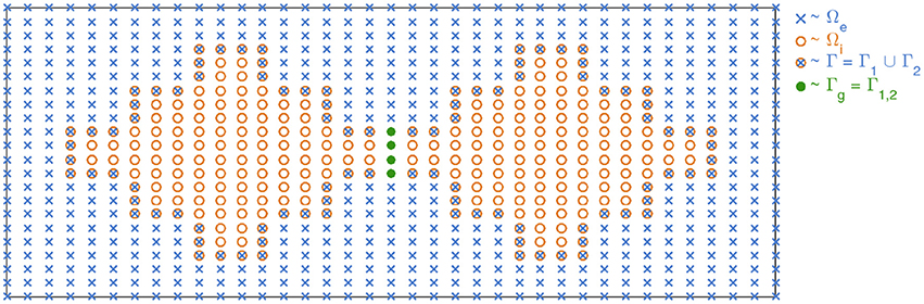
Figure 2. Sketch of the computational mesh used for the FDM. Nodes in Ω_e are marked by ×, nodes in ${\Omega }_i={\Omega }_i^1\cup {\Omega }_i^2$ are marked by ◦, nodes on the membrane between the intracellular and the extracellular space (Γ = Γ₁ ∪ Γ₂) are marked by ⊗, and nodes on the membrane between two cells (Γ_1,2) are marked by •.

We use the notation $u_e^{n,j,k}$ for the numerical solution of the extracellular potential, u_e, at the point (x_j, y_k) = (jΔx, kΔy) at time t_n = nΔt and use an analogous notation for the numerical solution of the remaining variables.

We discretize (1) using the finite difference scheme

$\begin{array}{l}\frac{{\sigma }_e^{j+1/2,k}(u_e^{n,j+1,k}-u_e^{n,j,k})-{\sigma }_e^{j-1/2,k}(u_e^{n,j,k}-u_e^{n,j-1,k})}{\Delta x^2}\\ +\frac{{\sigma }_e^{j,k+1/2}(u_e^{n,j,k+1}-u_e^{n,j,k})-{\sigma }_e^{j,k-1/2}(u_e^{n,j,k}-u_e^{n,j,k-1})}{\Delta y^2}=0,& (14)\end{array}$

where ${\sigma }_e^{j+1/2,k}={\sigma }_e((j+1/2)\Delta x,k\Delta y).$ Equation (2) is discretized similarly, with σ_e replaced by σ_i and u_e replaced by u_i.

On the membrane between the intracellular and extracellular domains, there are three unknowns and three equations. The first equation is given directly by (5) and the second equation is given by a first-order finite difference discretization of (4). Finally, the third equation is given by an implicit discretization of (6) of the form

$\begin{array}{ll}\frac{v^{n,j,k}-v^{n-1/2,j,k}}{\Delta t}=\frac{1}{C_m}{I}_m^{n,j,k},& (15)\end{array}$

where $I_m^{n,j,k}$ is a discrete version of the term n_e · σ_e∇u_e from (4) and v^{n−1/2, j, k} is the solution of the membrane potential from the first step of the operator splitting procedure.

Similarly, for the nodes on the membrane between the cells, there are three unknowns and three equations. The first equation is given directly by (8), the second is a first-order finite difference discretization of (7), and the third is an implicit discretization of (9) of the form

$\begin{array}{ll}\frac{w^{n,j,k}-w^{n-1,j,k}}{\Delta t}=\frac{1}{C_{1,2}}\left(I_{1,2}^{n,j,k}-I_{\text{gap}}(w^{n,j,k})\right),& (16)\end{array}$

where $I_{1,2}^{n,j,k}$ is a discrete version of the term $n_i^2·{\sigma }_i\nabla u_i^2$ from (7) and $I_{\text{gap}}(w^{n,j,k})$ is a linear function of w^{n, j, k} given by (13). It is worth mentioning here that if the gap junction dynamics is modeled using a non-linear model, operator splitting can be applied as was done for the membrane model.

Two special types of nodes require some special treatment. The first type is the nodes on the corners of the membrane. For these nodes, we define two flux terms $I_m^{n,j,k}=n_e·{\sigma }_e\nabla u_e$, one for the normal derivative in the x direction and one for the normal derivative in the y direction, and we use the mean of these two terms in the equation of the form (15). Furthermore, in the flux equality Equation (4), we also define two intracellular flux terms, one for each direction, and let the sum of the two intracellular flux terms equal the sum of the two extracellular flux terms.

The second special node type is the extracellular nodes located next to a node on the membrane between two cells. In Figure 2, these are the two extracellular nodes just above or below Γ_1,2. For these nodes, we define a no-flux boundary condition between the extracellular node and the adjacent node on Γ_1,2. This is implemented by defining an extracellular potential for the node on the end of Γ_1,2 with a value equal to the extracellular potential in the node just outside Γ_1,2.

When considering a linear model for I_ion, we skip the first step of the operator splitting procedure and replace the equation of the form (15) in the finite difference scheme by

$\begin{array}{ll}\frac{v^{n,j,k}-v^{n-1,j,k}}{\Delta t}=\frac{1}{C_m}\left(I_m^{n,j,k}-I_{\text{ion}}(v^{n,j,k})\right).& (17)\end{array}$

A major drawback of the finite difference discretization is the fact that actual cell geometries are quite complex and virtually impossible to handle with this method. However, complex geometries can be resolved by the finite element method. In the following, we shall propose two different FEM formulations of the EMI Equations (1–9): the mortar finite element formulation, where the primary unknowns are the intra/extracellular potentials, and the H(div)-based finite element formulation, where the currents are the primary unknowns in the cells/tissue.

2.3.2. Mortar Finite Element Method for Solving the EMI PDEs

Mortar finite element methods ([51]; see also [4] for the application of the method in simulations of cell membranes) allow for the coupling of different types of variational problems posed over non-overlapping domains by weakly (in an integral sense) enforcing interface conditions on common boundaries. For the EMI system, the Poisson problems (1) and (2) are coupled by the conditions (4) and (5) and the conditions (7) and (8).

Let V_e and $V_i^k$ be spaces of functions over Ω_e and ${\Omega }_i^k$ for k = 1, 2, and let Q be a function space defined over Γ = Γ₁ ∪ Γ₂ ∪ Γ_1,2, to be precisely defined below. For any ψ ∈ Q, we denote by ψ¹, ψ² and ψ^1,2 the restriction of ψ to Γ₁, Γ₂, and Γ_1,2, respectively. With this notation, given (v^k)ⁿ and wⁿ at time level n, at each time level n+1 of the temporal discretization, we aim to find the membrane current density J ∈ Q, defined such that $J^k=I_m^k$ and $J^{1,2}=I_{1,2}$ and the extracellular and intracellular potentials u_e ∈ V_e and $u_i^i\in V_i^k$ such that:

$\begin{array}{ll}\begin{array}{c}{\displaystyle {\int }_{{\Omega }_i^1}}{\sigma }_i\nabla u_i^1·\nabla {\varphi }_i^1\text{d}x+{\displaystyle {\int }_{{\Gamma }_1}}{J}^1{\varphi }_i^1\text{d}s+{\displaystyle {\int }_{{\Gamma }_{1,2}}}{J}^{1,2}{\varphi }_i^1\text{d}s=0\forall {\varphi }_i^1\in V_i^1,\hfill \\ {\displaystyle {\int }_{{\Omega }_i^2}}{\sigma }_i\nabla u_i^2·\nabla {\varphi }_i^2\text{d}x+{\displaystyle {\int }_{{\Gamma }_2}}{J}^2{\varphi }_i^2\text{d}s-{\displaystyle {\int }_{{\Gamma }_{1,2}}}{J}^{1,2}{\varphi }_i^2\text{d}s=0\forall {\varphi }_i^2\in V_i^2,\hfill \\ {\displaystyle {\int }_{{\Omega }_e}}{\sigma }_e\nabla u_e·\nabla {\varphi }_e\text{d}x-{\displaystyle {\int }_{{\Gamma }_1}}{J}^1{\varphi }_e\text{d}s-{\displaystyle {\int }_{{\Gamma }_2}}{J}^2{\varphi }_e\text{d}s=0\forall {\varphi }_e\in V_e,\hfill \\ {\displaystyle {\int }_{{\Gamma }_1}}(u_i^1-u_e){\psi }^1\text{d}s-\frac{\Delta t}{C_m}{\displaystyle {\int }_{{\Gamma }_1}}{J}^1{\psi }^1\text{d}s={\displaystyle {\int }_{{\Gamma }_1}}{(v^1)}^n{\psi }^1\text{d}s\forall \psi \in Q,\hfill \\ {\displaystyle {\int }_{{\Gamma }_2}}(u_i^2-u_e){\psi }^2\text{d}s-\frac{\Delta t}{C_m}{\displaystyle {\int }_{{\Gamma }_2}}{J}^2{\psi }^2\text{d}s={\displaystyle {\int }_{{\Gamma }_1}}{(v^2)}^n{\psi }^2\text{d}s\forall \psi \in Q,\hfill \\ {\displaystyle {\int }_{{\Gamma }_{1,2}}}(u_i^1-u_i^2){\psi }^{1,2}\text{d}s-\frac{\Delta t}{C_{1,2}}{\displaystyle {\int }_{{\Gamma }_{1,2}}}{J}^{1,2}{\psi }^{1,2}\text{d}s={\displaystyle {\int }_{{\Gamma }_{1,2}}}{w}^n{\psi }^{1,2}\text{d}s\forall \psi \in Q.\hfill \end{array}\hfill & (18)\end{array}$

Here, the first three equations of the variational problem are obtained by multiplying (1) and (2) by test functions ϕ_e and ${\varphi }_i^k$ and integrating over the associated domains while using conditions (4) and (7) in the integration by parts. The final three equations are then weakly enforcing the constraints

$\begin{array}{ll}{u}_i^k-u_e-\frac{\Delta t}{C_m}{I}_m^k={(v^k)}^n\mathrm{\text{ on}}{\Gamma }_i^k,u_i^1-u_i^2-\frac{\Delta t}{C_{1,2}}{I}_{1,2}=w^n\mathrm{\text{ on}}{\Gamma }_{1,2}& (19)\end{array}$

which are obtained by a backward Euler discretization of (6) and (9) (cf. Equations 15 and 16) while expanding the transmembrane potentials of ${\Gamma }_i^k$ and Γ_1,2 at the (n+1)th temporal level using definitions (5) and (8), respectively. We note that the definitions of the transmembrane potentials enter the variational problem only via (19). Moreover, the membrane current density J can be interpreted as the multiplier of the augmented Lagrangian associated with these constraints.

System (18) is the linear part of the operator splitting procedure described above. The well-posedness of the system (18) was established in Belgacem [52] or Lamichhane [53] for the stationary case, where it was shown that a unique solution exists in the Sobolev spaces $V_e=H_{0,\partial {\Omega }_e}^1({\Omega }_e)$, $V_i^k=H^1({\Omega }_i^k)$ and Q = H^−1/2(Γ).

To discuss the finite element discretization of the well-posed problem (18), we denote by ${{T}}_{e,h}$ and ${{T}}_{i,h}^k$ simplicial meshes of the domains Ω_e and ${\Omega }_i^k$, respectively. Generally, the mortar finite element approach allows the tessellations to be independent of one another and the elements of Γ_h, the triangulation of Γ, are defined in terms of facets of one of the sharing tessellations. For simplicity, we opt here for meshes such that they share facets on Γ (see Figure 3). In particular, the neighboring tessellations define identical meshes Γ_h.

FIGURE 3

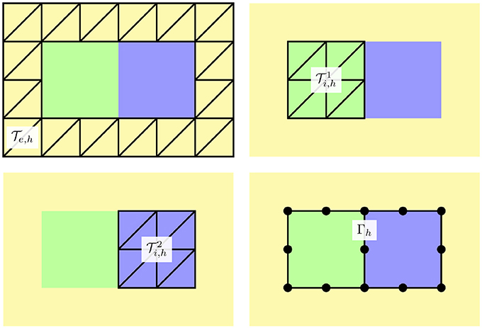
Figure 3. Schematic representation of finite element meshes considered with the mortar element method: (upper left) the tesselation ${{T}}_{e,h}$ of the extracellular domain, (upper right and bottom left) the tessellations ${{T}}_{i,h}^1$ and ${{T}}_{i,h}^2$ of the intracellular domains, and (bottom right) the membrane discretization Γ_h. In our implementation, ${{T}}_{e,h}$ and ${{T}}_{i,h}^k$ have identical facets on Γ and the facets define the finite element cells of Γ_h, see the location of the vertices of the 1D mesh depicted by black circles.

In the following, the discrete finite element subspaces of V_e, $V_i^k$, and Q will be constructed from continuous piecewise linear Lagrange elements. More precisely, we let

$\begin{array}{l}\begin{array}{c}{V}_{e,h}=\left\{v\in C({{T}}_{e,h});v{|}_K=P^1(K)\forall K\in {{T}}_{e,h}\right\},\\ V_{i,h}^k=\left\{v\in C({{T}}_{i,h}^k);v{|}_K=P^1(K)\forall K\in {{T}}_{i,h}^k\right\},\\ Q_h=\left\{v\in C({\Gamma }_h);v{|}_K=P^1(K)\forall K\in {\Gamma }_h\right\}\end{array}\end{array}$

and thus the space Q_h is the trace space of the functions in V_e,h and $V_{i,h}^k$. We refer to Wohlmuth [54] and references therein for proof of the numerical stability of this choice of discretization. We also note that the choice of element for the space Q_h simplifies the implementation, however, dual Lagrange multipliers (see [53, 54]), though more involved, are more suitable if static condensation is employed to solve the linear system arising from (18). Finally, in the numerical experiments, the scheme was implemented using the FEniCS_ii extension [55] of the FEniCS finite element library [49, 50].

2.3.3. H(div)-Based Finite Element Method for Solving the EMI PDEs

The mortar finite element formulation defined above introduces separate function spaces for each of the intracellular domains ${\Omega }_i^k$, which adds implementational complexity. As an alternative approach, we also consider an H(div)-based finite element method (e.g., [56]) for solving the PDE step of the operator splitting scheme. This scheme relaxes the continuity constraint for the potentials throughout the domain Ω and introduces potential gradients as additional variables with the appropriate normal continuity regularity for the associated currents. Therefore, the interface continuity conditions for the currents can be handled seamlessly.

To this end, we use the intracellular current density vector Ĵ_i and the extracellular current density vector Ĵ_e as additional vector fields defined over Ω_i and Ω_e, respectively:

$\begin{array}{ll}{Ĵ}_i=-{\sigma }_i\nabla u_i,{Ĵ}_e=-{\sigma }_e\nabla u_e.& (20)\end{array}$

We let Ĵ denote the extension of Ĵ_i and Ĵ_e to Ω, and assume that Ĵ is in the space H(div, Ω), that is, Ĵ is a square-integrable vector field with square-integrable divergence. Furthermore, denote by u the extension of u_i and u_e to Ω, and analogously for σ. In addition, we define $\widehat{v}$ as the extension of the transmembrane potential v and the transcellular potential w and we let Î denote the extension of I_ion and I_gap. Thus the variable u is defined over Ω while $\widehat{v}$ and Î are defined over the whole interior membrane $\widehat{\Gamma }={\Gamma }_1\cup {\Gamma }_2\cup {\Gamma }_{1,2}$.

Let n_i denote the outward normal, from the intracellular domains to the extracellular domain, on Γ_k for k = 1, 2 and from ${\Omega }_i^1$ to ${\Omega }_i^2$ on Γ_1,2 and, analogously, let n_e denote the outward normal from the extracellular to the intracellular domains. By the flux continuity conditions (4) and (7), we require that Ĵ_i · n_i = −Ĵ_e · n_e on Γ_k (k = 1, 2) and analogously on Γ_1,2. Let ${\widehat{v}}^{n,*}$ denote the membrane potential solution from the ODE step in the nonlinear case or the membrane solution ${\widehat{v}}^{n,*}={\widehat{v}}_h^{n-1}$ at the previous time in the linear (no ODE) case.

With this notation and after an implicit Euler discretization in time, our H(div)-based finite element scheme at each time step n reads as follows: For given v^n,*, fⁿ, and gⁿ, find $u_h^n\in U_h$, ${Ĵ}_h^n\in S_h$ and ${\widehat{v}}_h^n\in V_h$ such that

$\begin{array}{ll}-{\displaystyle {\int }_{\Omega }}\nabla ·{Ĵ}_h^n\varphi \text{d}x={\displaystyle {\int }_{\Omega }}{f}^n\varphi \text{d}x\forall \varphi \in U_h,& (21)\end{array}$

$\begin{array}{l}{\displaystyle {\int }_{\Omega }}\left({\sigma }^{-1}{Ĵ}_h^n·\tau -\nabla ·\tau u_h^n\right)\text{d}x+{\displaystyle {\int }_{\widehat{\Gamma }}}\tau ·n_i{\widehat{v}}_h^n\text{d}s\\ ={\displaystyle {\int }_{\Omega }}{g}^n·\tau \text{d}x\forall \tau \in S_h,& (22)\end{array}$

$\begin{array}{l}{\displaystyle {\int }_{\widehat{\Gamma }}}\left(C_m{\widehat{v}}_h^n+\Delta t(-{Ĵ}_h^n·n_i+\alpha Î({\widehat{v}}_h^n))\right)\beta \text{d}s\\ ={\displaystyle {\int }_{\widehat{\Gamma }}}{C}_m{\widehat{v}}^{n,*}\beta \text{d}s\forall \beta \in V_h.& (23)\end{array}$

In the case of a nonlinear I_ion, we set α = 0 and treat the non-linear term by operator splitting as outlined above.

In the numerical experiments, as for the mortar finite element method described in section 2.3.2, we let ${{T}}_h$ denote a simplicial mesh of Ω conforming to ${\Omega }_i^k$ (k = 1, 2) and Ω_e such that ${\widehat{\Gamma }}_h$, the restriction of ${{T}}_h$ to $\widehat{\Gamma }$, defines a conforming mesh of $\widehat{\Gamma }$ (of one topological dimension lower). Relative to these meshes, we define the spaces S_h as the lowest-order Raviart–Thomas elements defined over ${{T}}_h$ and U_h as the space of (discontinuous) piecewise constants defined over ${{T}}_h$, and V_h as the space of (discontinuous) piecewise constants defined over ${\widehat{\Gamma }}_h$. The Raviart–Thomas elements are, by definition, such that the normal components of the vector fields are continuous across cell facets (edges in 2D, faces in 3D) and thus the flux continuity conditions (4) and (7) hold by construction [56].

This mixed finite element combination is conforming and our numerical experiments indicate that the element pairing is stable and convergent. The scheme can also be compared to the schemes discussed by Sacco [57]. Based on the interpolation properties of the lowest-order finite element spaces as described above, we expect to observe first-order convergence for u, Ĵ, and $\widehat{v}$ in the respective L² norms, and first-order convergence for Ĵ in the H(div) norm. Higher-order convergence in the L² norm of Ĵ can be recovered by using the Brezzi–Douglas–Marini [58] H(div) elements instead of the Raviart–Thomas family.

In the numerical experiments, this scheme was implemented using the FEniCS finite element library [49, 50].

2.4. Optimal Solvers

A common problem in scientific computing is to solve a linear PDE defined on a certain geometry. After applying some sort of discretization characterized by a mesh parameter h, the remaining problem is to solve a linear system of algebraic equations. The linear solution process is usually said to be order optimal provided that the number of floating point operations (FLOPs) required to solve the problem grows linearly in the number of unknowns as h decreases. For self-adjoint, linear PDEs, optimal solvers are well understood (e.g., see the review papers [59, 60] for the theory of saddle point problems). In simulating cardiac tissue, optimal solvers exist for both the monodomain model and the bidomain model (e.g., [11, 61, 62]).

Feynman [63] suggested an alternative, but related, definition of order optimality: Suppose a numerical method is used to simulate a small space–time volume of a physical process and the mesh is refined to convergence. Then computational complexity should only grow linearly as the space–time volume is increased. For our application, this definition is very well suited; we consider a single cell surrounded by an extracellular space, and we carry out numerical simulations to find the mesh resolution in time and space necessary to obtain convergence. Then we define a numerical solution as being order optimal provided that the CPU efforts only increase linearly in the number of biological cells in the computation.

3. Results

In this section, we present applications of the methods introduced above. We start by assessing the accuracy of the numerical methods for a very simple unitless test problem where an analytical solution can be enforced using the method of manufactured solutions. For non-linear membrane dynamics, we explore convergence under mesh refinements. Next, we consider the CPU efforts needed to solve the numerical problems arising from the EMI model and we are particularly interested in the CPU effort per physical cell to understand the scalability of the EMI approach. For the FEM, we also show results for cylindrical geometries. Finally, we investigate the effect of non-uniform distributions of sodium channels along the cell membrane.

3.1. Model Parameters

In the first unitless test problem we consider a 2D domain consisting of an extracellular domain and a single cell. In the remaining simulations, we consider 3D domains consisting of a number of connected cells and the surrounding extracellular space. The coupled cells are organized as a single layer where the cells are connected to each other in a grid in the x and y directions by gap junctions. The shape and size of the cells and the extracellular domain will be specified for each simulation below. We primarily consider cells of the shape illustrated in Figure 4, where each part of the intracellular domain, Ω_O, Ω_W, Ω_E, Ω_S, and Ω_N, is shaped as a rectangular cuboid.

FIGURE 4

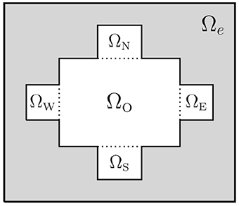
Figure 4. Sketch of the 2D version of a domain in the case of a single cell. Here, Ω_i = Ω_O ∪ Ω_W ∪ Ω_E ∪ Ω_S ∪ Ω_N.

The parameter values used in the simulations are given in Table 1 unless otherwise specified. Moreover, we use the initial condition w = 0 in all the simulations of connected cells. When the Grandi model is used to model I_ion, we mainly use the default initial conditions of the Grandi model for v and the remaining state variables. When a passive model is used for I_ion, we primarily use the initial condition v = v_rest.

TABLE 1

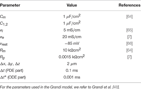
Table 1. Default parameter values used in the simulations.

3.2. Numerical Verification and Accuracy

3.2.1. Linear Ionic Current: Method of Manufactured Solutions

To evaluate the accuracy of the numerical methods, we construct an analytical solution for a 2D single-cell version of the EMI model with the passive model I_ion = v. The analytical solution of this simple example is constructed using the method of manufactured solutions (e.g., [67]). We consider a single cell surrounded by extracellular space:

$\begin{array}{ll}\nabla ·{\sigma }_i\nabla u_i=f,\text{in}{\Omega }_i,& (24)\end{array}$

$\begin{array}{ll}\nabla ·{\sigma }_e\nabla u_e=g,\text{in}{\Omega }_e,& (25)\end{array}$

$\begin{array}{ll}{u}_e=0,\text{at }\partial {\Omega }_e,& (26)\end{array}$

$\begin{array}{ll}{n}_e·{\sigma }_e\nabla u_e=-n_i·{\sigma }_i\nabla u_i,\text{at}\Gamma ,& (27)\end{array}$

$\begin{array}{ll}{u}_i-u_e=v,\text{at}\Gamma ,& (28)\end{array}$

$\begin{array}{ll}{I}_m=-n_i·{\sigma }_i\nabla u_i,\text{at}\Gamma ,& (29)\end{array}$

$\begin{array}{ll}{v}_t=\frac{1}{C_m}(I_m-I_{\text{ion}}),\text{at}\Gamma .& (30)\end{array}$

For this case, we assume that the model is unitless with parameters σ_i = σ_e = C_m = 1, and we define the domain Ω = Ω_i ∪ Ω_e = [0, 1] × [0, 1], where Ω_i = [0.25, 0.75] × [0.25, 0.75].

We let

$\begin{array}{ll}f=f(x,y,t)=-8{\pi }^{2}sin(2\pi x)sin(2\pi y)(1+e^{-t}),& (31)\end{array}$

$\begin{array}{ll}g=g(x,y,t)=-8{\pi }^{2}sin(2\pi x)sin(2\pi y)& (32)\end{array}$

and the analytical solution of (24–30) is then given by

$\begin{array}{ll}{u}_i(x,y,t)=(1+e^{-t})sin(2\pi x)sin(2\pi y),& (33)\end{array}$

$\begin{array}{ll}{u}_e(x,y,t)=sin(2\pi x)sin(2\pi y),& (34)\end{array}$

$\begin{array}{ll}v(x,y,t)=e^{-t}sin(2\pi x)sin(2\pi y).& (35)\end{array}$

In the numerical experiments of this test case, we use Δt = 0.01/n, where for the FDM, n equals the number of intervals in each direction of the spatial discretization of the domain. In the FEM case, 2n² is the number of triangles that constitute the uniformly discretized mesh. We note that the chosen time step criterion is not necessary for numerical stability of any of the methods. Rather, it was selected to yield more stable convergence rates. For this test case, the linear systems arising in the experiments are solved by direct solvers (LU factorization), and the errors are computed at time t = 0.1.

Table 2 shows the maximum error of the finite difference method as the discretization parameters are refined. We observe that the convergence rates of the intracellular and extracellular potentials u_h and the membrane potential v_h are both close to one, indicating that the maximum (L^∞) error of the FDM is O(h).

TABLE 2

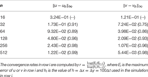
Table 2. Convergence of the finite difference method for the manufactured test problem with convergence rates in parentheses.

In Table 3, we report the results obtained with the mortar FEM. The error of the potentials u_h is reported in the broken H¹ norm ||u−u_h||₁, which is natural for the problem [53], the L² norm ||u−u_h||₀ to enable comparison with the H(div) FEM, and the supremum norm ||u−u_h||_∞ to allow for comparison across different numerical methods. The error in the current density J_h is measured in the L² norm rather than the natural but more involved H^−1/2 norm. Finally, we report convergence of the membrane potential difference ||v−v_h||_∞, where v_h is obtained from the definition u_i,h − u_e,h = v_h using the computed potentials. We note that the integral norms are evaluated by first interpolating the error in the space of discontinuous fourth-order polynomials. The supremum norms are then computed using linear polynomials.

TABLE 3

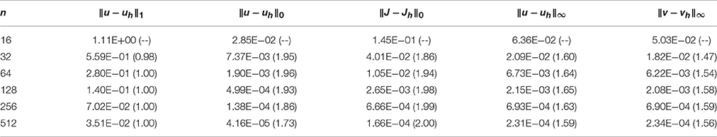
Table 3. Convergence of the mortar finite element method for the manufactured test problem, with convergence rates in parentheses.

Using piecewise linear elements, the observed convergence rates in the integral norms (see the first three columns of Table 3), are 1.0 (optimal) and 1.73 (slightly suboptimal) for the broken H¹ norm and the L² norm of potentials, respectively, while order 2 can be seen in the L² norm of the current density. We note that the suboptimal rate of convergence is due to the error being dominated by the temporal discretization and decreasing the time step restores the optimal quadratic convergence. Let us also note that the quadratic convergence of the current density is likely related to the fact that I_m = 0 in the test case. The observed order of convergence in the supremum norms is 1.59 and 1.56 for u_h and v_h, respectively. However, the error here seems again to be dominated by temporal discretization, since using Δt = 10⁻³/n improves the rates toward 2.0.

Table 4 reports the errors and convergence rates for the H(div)-based FEM. The error in the computed intracellular and extracellular potentials u_h and the error in the membrane potential v_h are reported in the L² norm and in the supremum norm. Furthermore, the error in the computed potential gradient Ĵ_h is reported in the L² and H(div) norms. We observe that the convergence rate is one both for the error in the L² norm for u_h and v_h and for the H(div) and L² norms for Ĵ_h. These rates are in complete agreement with the theoretical expectations. In addition, we observe that the convergence of the supremum norm of u_h and v_h, computed after a projection onto continuous piecewise linears, appears to be close to quadratic.

TABLE 4

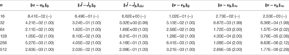
Table 4. Convergence of the H(div) finite element method for the manufactured test problem, with convergence rates in parentheses.

3.2.2. Nonlinear Ionic Current: Mesh Refinement

To investigate the accuracy of the numerical methods using the Grandi AP model, we compare the solutions obtained from the numerical methods using different spatial resolutions.

Figure 5 shows the solution of the membrane potential in a single point on the membrane for the FDM and the H(div)-based FEM for a number of resolutions. We consider the solution for two connected cells; and the sizes of the cells and the domain used in the simulations are given in Table 5.

FIGURE 5

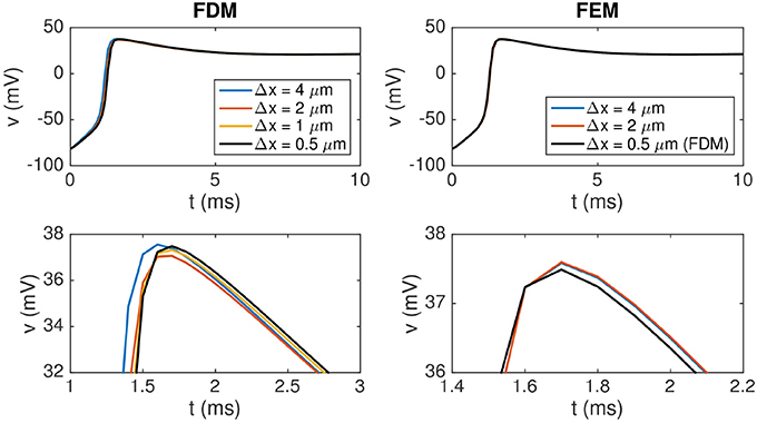
Figure 5. Membrane potential at the point (112, 24, 16 μm) for the finite difference and the finite element methods for two connected cells for some different values of Δx = Δy = Δz. The upper panel shows the solution from t = 0 ms to t = 10 ms. In the lower panel, we zoom in on the peak to observe a difference between the solutions. Note that the scaling of the y axis is different for the two plots in the lower panel and that the FEM solutions for Δx = 4 μm and Δx = 2 μm are almost indistinguishable in the lower right plot. The parameter values used in the simulations are given in Tables 1, 5, and we apply a 1-ms-long stimulus current of 120 μA/μF for the first 24 μm of the first cell.

TABLE 5

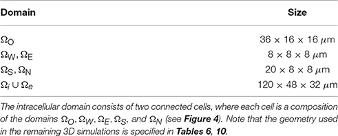
Table 5. The cell and domain sizes used in the simulations reported in Figure 5.

In the upper panel of Figure 5, the solutions for different resolutions are almost indistinguishable, but in the lower panel we focus on a small part of the solution and a difference is visible for the different resolutions of the FDM. The H(div) FEM solutions are very similar for different resolutions, indicating that the method is more accurate than the FDM in this case as well.

3.3. CPU Requirements

As mentioned in the section 1, simulation of the electrophysiology of cardiac tissue is usually based on homogenized models such as the monodomain model or the bidomain model. The motivation for this is certainly that it requires considerably less computing power than the EMI approach considered here. Therefore, it is very important to understand the computational complexity of the EMI model to appreciate the applications in which this approach can be used.

3.3.1. Finite Difference Method

Tables 7, 8 report the CPU times, number of iterations, and system size for the FDM as the number of cells included in the simulation is increased. In Table 7, we use the passive model (10) for I_ion, and in Table 8, we use the Grandi AP model. The linear systems are solved using the BiCGStab method (see [68, 69]) with an incomplete LU preconditioner (e.g., [68]) and relative tolerance of 10⁻⁵ for the true/unpreconditioned (l²) norm of the residuum. The computations are performed using MATLAB. The last column of the tables reports the simulation time per cell for a single time step and we observe that the simulation time per physical cell appears to be bounded as the number of cells is increased.

TABLE 6

Table 6. Cell sizes used in the simulations reported in Figures 7–9 and Tables 7–9.

TABLE 7

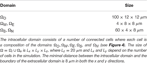
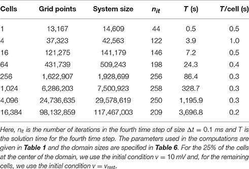
Table 7. CPU times for the finite difference method for a passive membrane model.

TABLE 8

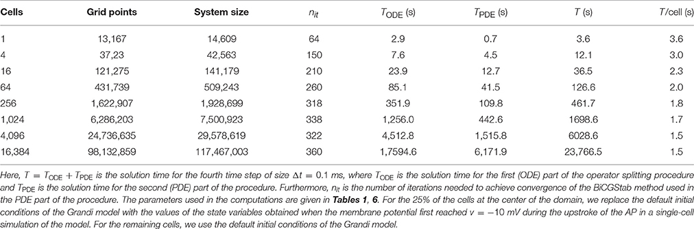
Table 8. CPU times for the finite difference method using the Grandi membrane model for I_ion.

3.3.2. Finite Element Method

Because of the complexity of the mortar FEM, which introduces a separate function space for the potential of each cell¹ ${\Omega }_i^k$, we shall focus on the H(div) FEM in the following.

Table 9 shows the CPU time, the number of iterations, and the dimensions of the finite element spaces for a number of simulations using the H(div) FEM described in section 2.3.3 with an increasing number of cells and a passive membrane model. The linear systems are again solved using the biconjugate gradient stabilized method with an incomplete LU preconditioner and a convergence criterion as in the FDM case. The linear solver and the preconditioner were provided by the PETSc library [70], while the system was assembled using FEniCS [49, 50].

TABLE 9

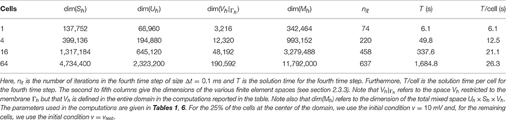
Table 9. CPU times for the H(div) finite element method for a passive membrane model.

Since the definition of the H(div)-based variational problem (21) in FEniCS is not immediately obvious, we briefly comment on some implementational aspects. Recall that the solution is sought in the space U_h × S_h × V_h, where the functions in V_h are defined over ${\widehat{\Gamma }}_h$, the discretization of the cell mebranes Γ. However, FEniCS (version 2017.1) does not currently support mixed spaces with components defined over different meshes, such as over ${{T}}_h$ and ${\widehat{\Gamma }}_h$. To bypass this restriction, we construct the space V_h over all the facets of ${{T}}_h$ and the excess degrees of freedom are set to zero in the assembled linear system. As illustrated above the construction yields the correct numerical solution. However, the additional degrees of freedom naturally affect the performance of the linear solvers, since they increase the computational cost of the matrix–vector product significantly. FEniCS support for mixed finite element spaces with components defined over different meshes is currently under development and we thus expect this issue to be resolved in future FEniCS releases.

Comparing the results of Table 9 with those of the FDM (see Table 7), we observe that the CPU times for the FEM are considerably larger (by a factor of ~70). While the longer solution times for the FEM are expected due to the larger linear systems stemming from the method (with factors of ~23 and ~14 for the system with or without the additional degrees of freedom introduced in V_h, respectively), the results also point out that the iterative solver does not perform as well as in the FDM case. More efficient solution strategies for the system are currently being investigated.

3.4. Cylindrical Geometry

The somewhat clunky geometry of the cells used above does not reflect reality very well. Indeed, cardiac cells have cylindrical shapes, but such shapes are inconvenient to address using FDMs, and we therefore apply the FEM. Figure 6 shows the membrane potential and surrounding extracellular potential for a simulation of two connected cylinders using the parameters given in Tables 1, 10. We note that the FEM is well suited for handling cylindrical geometry, and we expect that the method can also be used to handle the even more complex geometries that will arise when the T-tubules of ventricular cells (e.g., [71]) are incorporated in the model.

FIGURE 6

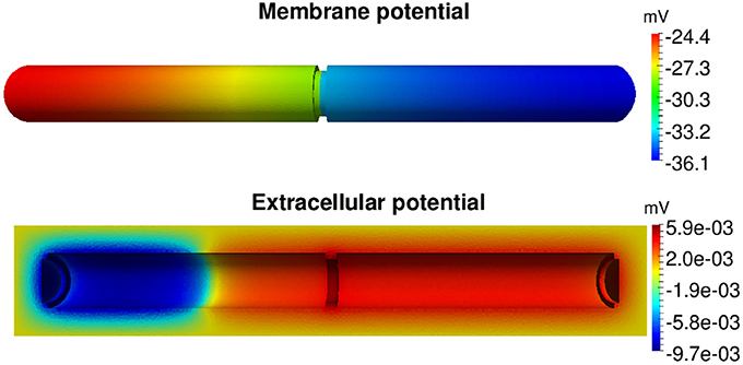
Figure 6. Membrane potential and the surrounding extracellular potential of two connected cylinders at time t = 1 ms computed by the H(div) FEM. The parameters used in the simulations are given in Tables 1, 10 and we apply a stimulus current of 120 μA/μF for the first half of the first cell in the x direction.

TABLE 10

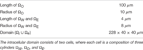
Table 10. Cell and domain sizes used in the simulations of the two connected cylinders in Figure 6.

3.5. Ion Channel Density Distribution Affects Conduction Velocity

As mentioned in the section 1, it is difficult to represent a non-uniform distribution of ion channels along the cell membrane using classical homogenized models. This is an important shortcoming of the classical methods, because a non-uniform distribution of sodium channels is believed to affect the conduction velocity. In the EMI modeling framework, the representation of non-uniform distributions of ion channels is straightforward.

Figure 7 shows the solutions of two simulations of a collection of 30 × 5 cells with different distributions of the sodium channel conductance, g_Na. In the left panel the value of g_Na is constant on the entire membrane, while, in the right panel, g_Na is zero over a large part of the membrane and only non-zero on Ω_W and Ω_E, that is, near the ends of the cell in the x direction. The mean value of g_Na over the cells is the same in the two simulations. We observe that the conduction velocity is increased for the case with a varying value of g_Na compared to the case with a constant value. The conduction velocities reported in the figure are computed from the 10th and 20th cells in the third row in the y direction, and are defined as the distance between the cell centers divided by the time between each of the two cell centers reaches a membrane potential of v = 0 mV.

FIGURE 7

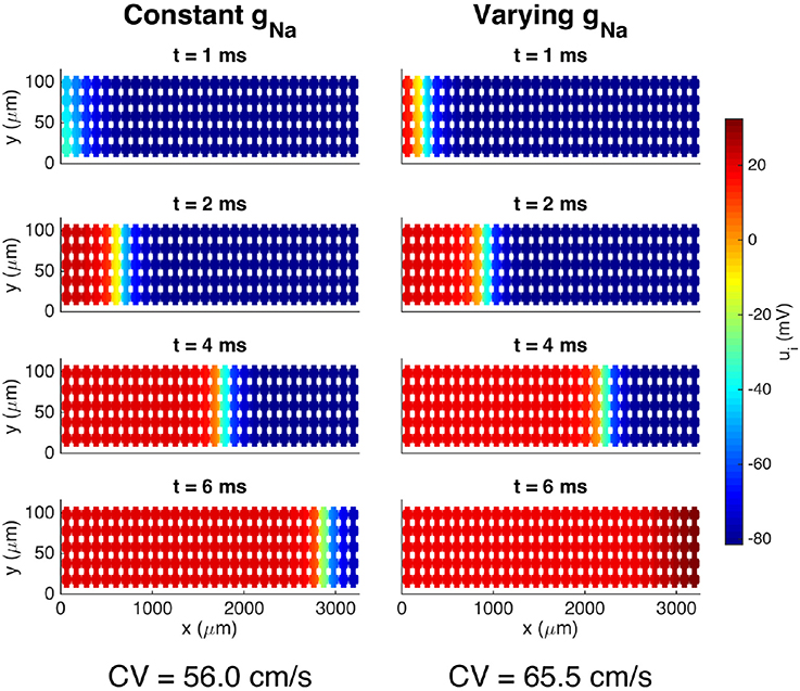
Figure 7. Intracellular potential at four points in time for a collection of cells with two different distributions of the sodium channel conductance. In the case of a constant g_Na, the value is g_Na = 23 mS/μF on the entire membrane, and in the case of a varying g_Na, the value is g_Na = 783 mS/μF on Ω_W and Ω_E and zero elsewhere. The solutions are obtained using the FDM and the parameters used in the simulations are given in Tables 1, 6, except that we use Δt = 0.01 ms. We apply a 1-ms-long stimulus current of 120 μA/μF for the 2 × 2 cells in the lower left corner of the domain.

Figure 8 shows a more detailed view of the two cells at the center of the domain. Here, we observe that the conduction velocity across the first part of the cell appears to be higher for the case with a constant value of g_Na than for the varying case, but that the traveling wave moves faster across the gap junction for the case with a varying g_Na than for the constant case, leading to an overall increased conduction velocity for the varying case.

FIGURE 8

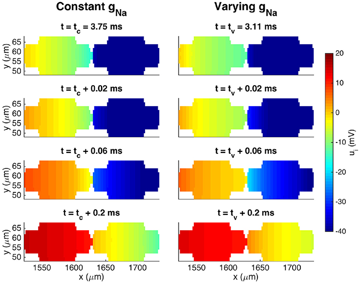
Figure 8. Intracellular potentials at four points in time for the two cells at the center of the domain from the simulation in Figure 7. The plots in the upper panel show the solutions at the last point in time before the intracellular potential at the start of the first cell is first positive. Because the conduction velocity is different in the two cases, this occurs at two different points in time, t_c and t_v, for the cases with a constant g_Na and a varying g_Na, respectively. The next plots show the solutions at times 0.02, 0.06, and 0.2 ms after t_c and t_v.

This effect is studied more closely in Figure 9, which shows the activation times and conduction velocities along the length of two cells in a similar pair of simulations. The gap junction between the two cells is located at x = 548μm, and we observe that there is a delay of about 0.1 ms between when the membrane on each side of the gap junction is activated. The delay appears to be slightly longer for the case with a constant g_Na compared to the varying case. We also observe that, overall, the wave uses less time to activate the two cells for the case with a varying g_Na than for the constant case, consistent with the results of Figures 7, 8. In addition, we observe that the shape of the activation curve is different in the two cases. In the case with a constant g_Na distribution, the activation curve becomes steeper toward the end of the cells, corresponding to a decreasing conduction velocity along the cell lengths. For the varying case, however, the activation curve flattens out toward the end of the cells, corresponding to an increased conduction velocity toward the cell ends.

FIGURE 9

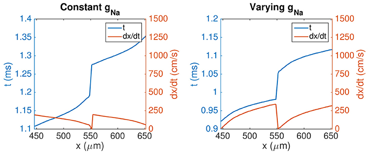
Figure 9. Activation times and conduction velocities along the length of two cells in a simulation of 10 × 1 cells with different distributions of g_Na, similar to the simulations shown in Figure 7. The blue line shows the points in time when the membrane nodes corresponding to each x-value along cells number five and six first reach a membrane potential of 0 mV. The orange line shows the corresponding conduction velocity along the two cells, computed from a piecewise second order polynomial approximation of the activation curves. The parameters used in the simulations are given in Tables 1, 6, except that we use Δt = 0.0005 ms. Note that the values of the left y-axis (representing activation time) is different in the two plots, but that the scaling of the axis is the same in both plots.

4. Discussion

As described above, the classical models of cardiac tissue are founded on homogenization of the tissue and the resulting models therefore assume that the extracellular space, the cell membrane, and the intracellular space exist everywhere. This leads to tractable computing problems that have provided insights into important applications such as the propagation of an electrochemical wave, cardiac arrhythmias, the effect of defibrillation, the onset of cardiac waves, and the effect of diverse drugs. However, in some cases, it is of interest to see the dynamics surrounding individual cells as part of the tissue, which is hard to do using homogenized models. It is also of interest to be able to change local properties of the tissue that are difficult to represent in homogenized models.

In the present report, we focused on the computational challenges of a different approach in which separate geometrical domains for the extracellular space, the cell membrane, and the intracellular domain represent the tissue; we refer to this as the EMI model. Clearly, the computational problems arising from the EMI model are much more challenging than for traditional models, but we have shown that, for some applications, the more detailed model is feasible. In particular, we have shown that the EMI model is suitable for monolayers of cells. Furthermore, we have demonstrated that the EMI framework allows the representation of local properties of cells that are hard to represent in classical homogenized models of cardiac tissue.

4.1. Membrane Dynamics

The dynamics of the cell membrane are absolutely critical for the functioning of the cell and have been subject to intense studies for centuries. A wide variety of models are available through the open CellML library [72]. In our computations, we have used the ventricular cell model by Grandi et al. [48]. That model consists of a system of 39 ODEs defined on every computational node of the cell membrane and is believed to provide an accurate representation of the cell's action potential. From a computational point of view, we could have used numerous other models (e.g., [73–80]) with comparable complexity of the membrane computations. Common to all these models is that the ion currents are represented using models where the ion channel density must be specified. When the models are used as part of a monodomain or bidomain model, the channel density is most conveniently treated as a constant for each cell, but in the EMI model, the ion channel density associated with any of the currents can be specified as a function of space on the cell membrane. We noted in Figure 7 that a non-uniform distribution of sodium channels significantly affects the tissue's conduction velocity.

4.2. Numerical Accuracy

The numerical accuracy of the discretizations considered was assessed using a single-cell problem (24–30) and the method of manufactured solutions. As seen in Tables 2–4, all the discretizations provide converging numerical solutions. However, taking the L^∞ norms of the computed potentials for comparison, there are considerable differences in the convergence properties of the methods.

The convergence of the FDM discretization is linear and this method is the least accurate. The first order convergence of the FDM is to be expected, since all internal boundary conditions are approximated using first-order finite differences. Compared to the FDM, the mortar FEM yields solutions with considerably smaller error and the observed rates are about 1.5. It should be noted that, on a given grid, the methods lead to identical numbers of unknowns. The H(div) FEM is the most accurate among the methods considered with errors much smaller than those of the mortar FEM. As noted in section 3.3, the H(div) FEM leads to larger linear systems than the other two methods do (see Tables 7, 9). Finally, let us note that the manufactured solution employed was particularly simple and thus the numerical results obtained may not be universally valid.

4.3. CPU Requirements

The CPU efforts needed to solve the system (1–9) using the FDM or the FEM are given in Table 7 (FDM, passive membrane dynamics), Table 8 (FDM, membrane dynamics given by the Grandi model), and Table 9 (H(div) FEM, passive membrane dynamics). We observe that, for the FDM, the CPU efforts per cell seem to be bounded independently of the number of cardiac cells. This result implies that the solver is optimal in the sense defined above. When the Grandi model is used for the membrane dynamics, the CPU efforts per time step per cell are around 1.5 s. This enables us to simulate 16,384 cells, which defines a linear system with over 117 million unknowns. Since the CPU efforts per cell seem to be bounded independent of the number of cells, the CPU efforts will not explode as more cells are added to the computations. With proper parallelization strategies, it should be possible to simulate huge numbers of cells. In fact, the mouse heart, with around 4 million cells, may be within reach; with a computer that is 1,000 times faster (for large problems) than the one we used, it would require about one week to perform 100 time steps for 4 million cardiac cells.

We observe from Tables 8, 9 that the FDM method in the current implementation is significantly faster than the FEM code even though the FDM code is implemented in Matlab. It has proven to be difficult to derive optimal preconditioners to be used for the FEM, but we hope to be able to improve this part of the code in the future.

4.4. Cell Geometry

In the present report, we have used very simple geometries to represent the cells. We have assumed that the geometries are simple rectangular cuboids or have cylindrical shapes. However, real cardiac cells have much more complex geometries and future work will investigate the effect of the geometry on the solutions. Of particular importance is the effect of T-tubules in ventricular cells and how they change during illness (e.g., [71, 81]). The diameter of the T-tubules ranges from 20 to 450 nm (see [82]) and therefore a very fine computational mesh would be needed to represent these invaginations. Presently, we have run the FDM code with spatial resolution of 5 nm (in the case of only three coupled cells), so including T-tubules is within reach for the FDM code but not for the FEM code.

4.5. Intracellular Calcium Dynamics

The focus of the present report has been to show that it is possible to simulate the electrical potential of cardiac cells based on explicit representation of the cells. We have focused on models that represent the membrane dynamics in terms of interchange over the cell membrane and we have ignored the spatial gradients of the ionic concentrations away from the cell membrane. Certainly, this is a major simplification; the intracellular concentration of calcium is essential and can be modeled using partial differential equations defined in the intracellular domain, see e.g. [83–86]. In Nivala et al. [83], a model based on Calcium released units (CRUs) is presented and the number of CRUs for a single cell used in the computations is typically ~20,000. In our model, a cardiac cell with a volume of 30 pL and a typical mesh length of 1 μm would consist of 30,000 computational blocks within each cell. A reasonable representation of the CRUs in the EMI model is therefore within reach.

4.6. Conduction Velocity

As mentioned above, the conduction velocity is essential for the stability of the electrochemical wave underpinning the rhythmic contraction of the cardiac muscle. In numerical computations, the distribution of ion channels is usually assumed to be constant, but experimental evidence suggests that the ion channel density is non-uniform along the cell membrane. For instance, the density of sodium channels is believed to be much higher closer to the intercalated discs separating individual cells (e.g., [87]). The difference between uniform and non-uniform distributions of sodium channels was addressed in Figures 7–9. We observed that the conduction velocity was significantly lower in the case of a constant distribution of the sodium channels compared to the case of a non-uniform distribution. Interestingly, we also observed (Figure 9) that for the uniform case, the conduction velocity decreased along the cell, whereas it increased in the case of non-uniform distribution. Again, such effects are difficult to observe in the classical models (monodomain, bidomain). This effect deserves closer scrutiny and the EMI model provides a suitable framework for such studies.

5. Conclusion

Local properties of cells and cell membranes are difficult to represent in standard (bidomain, monodomain) models of excitable tissue. In this paper, we have demonstrated that a more accurate model and method can be used. In our approach, every cell is represented in terms of its surrounding extracellular space, the cell membrane, and the intracellular space. The extracellular and intracellular spaces are represented using a mesh of length of 2μm and the membrane is represented as the intersection of the extracellular and intracellular meshes. We have seen that, with a finite difference method using a very simple geometry, the computations are quite efficient and the computational demands increase linearly in the number of physical cells. We have solved for up to 16,384 cells using this method. More complex geometries must be represented using a method allowing flexible grids and, in the present paper, we have shown the results for two variants of the finite element method. Although, the solution process of the finite element equations is much more time-consuming, the results indicate that more complex cell geometries can, in fact, be handled.

Author Contributions

Numerical methods: AT, KJ, MK, KM, MR. Software development: KJ, MK, MR. Simulations: AT, KJ, MK. Writing paper: AT, KJ, MK, KM, MR.

Funding

The research was supported by The Research Council of Norway through the grant 145739/F20.

Conflict of Interest Statement

The authors declare that the research was conducted in the absence of any commercial or financial relationships that could be construed as a potential conflict of interest.

Footnotes

1. ^The space for intracellular potentials for the case considered with FDM in the section 3.3.1 would be $V_i^1\times V_i^2\times \cdots \times V_i^n$ where n = 16, 384.

References

1. Hogues H, Leon L, Roberge F. A model study of electric field interactions between cardiac myocytes. IEEE Trans Biomed Eng. (1992) 39:1232–43.

PubMed Abstract | Google Scholar

2. Krassowska W, Neu JC. Response of a single cell to an external electric field. Biophys J. (1994) 66:1768.

PubMed Abstract | Google Scholar

3. Ying W, Henriquez CS. Hybrid finite element method for describing the electrical response of biological cells to applied fields. IEEE Trans Biomed Eng. (2007) 54:611–20. doi: 10.1109/TBME.2006.889172

PubMed Abstract | CrossRef Full Text | Google Scholar

4. Agudelo-Toro A, Neef A. Computationally efficient simulation of electrical activity at cell membranes interacting with self-generated and externally imposed electric fields. J Neural Eng. (2013) 10:026019. doi: 10.1088/1741-2560/10/2/026019

PubMed Abstract | CrossRef Full Text | Google Scholar

5. Stinstra JG, Henriquez CS, MacLeod RS. Comparison of microscopic and bidomain models of anisotropic conduction. In: Murray A, editor. Computers in Cardiology. IEEE (2009). p. 657–60.

Google Scholar

6. Stinstra JG, MacLeod RS, Henriquez CS. Incorporating histology into a 3D microscopic computer model of myocardium to study propagation at a cellular level. Ann Biomed Eng. (2010) 38:1399–414. doi: 10.1007/s10439-009-9883-y

PubMed Abstract | CrossRef Full Text | Google Scholar

7. Stinstra JG, Hopenfeld B, MacLeod RS. On the passive cardiac conductivity. Ann Biomed Eng. (2005) 33:1743–51. doi: 10.1007/s10439-005-7257-7

PubMed Abstract | CrossRef Full Text | Google Scholar

8. Tveito A, Jæger KH, Lines GT, Paszkowski Ł, Sundnes J, Edwards AG, et al. An evaluation of the accuracy of classical models for computing the membrane potential and extracellular potential for neurons. Front Comput Neurosci. (2017) 11:27. doi: 10.3389/fncom.2017.00027

PubMed Abstract | CrossRef Full Text | Google Scholar

9. Keener JP, Sneyd J. Mathematical Physiology. New York, NY: Springer (2009).

Google Scholar

10. Franzone PC, Pavarino LF, Scacchi S. Mathematical Cardiac Electrophysiology. Cham; Heidelberg; New York, NY; Dordrecht; London: Springer International Publishing (2014).

Google Scholar

11. Sundnes J, Nielsen BF, Mardal KA, Cai X, Lines GT, Tveito A. On the computational complexity of the bidomain and the monodomain models of electrophysiology. Ann Biomed Eng. (2006) 34:1088–97. doi: 10.1007/s10439-006-9082-z

PubMed Abstract | CrossRef Full Text | Google Scholar

12. Roth BJ. Bidomain simulations of defibrillation: 20 years of progress. Heart Rhythm (2013) 10:1218–9. doi: 10.1016/j.hrthm.2013.05.002

PubMed Abstract | CrossRef Full Text | Google Scholar

13. Trayanova NA. Whole-heart modeling: applications to cardiac electrophysiology and electromechanics. Circ Res. (2011) 108:113–28. doi: 10.1161/CIRCRESAHA.110.223610

PubMed Abstract | CrossRef Full Text | Google Scholar

14. Vigmond E, Vadakkumpadan F, Gurev V, Arevalo H, Deo M, Plank G, et al. Towards predictive modelling of the electrophysiology of the heart. Exp Physiol. (2009) 94:563–77. doi: 10.1113/expphysiol.2008.044073

PubMed Abstract | CrossRef Full Text | Google Scholar

15. Tveito A, Lines GT, Artebrant R, Skavhaug O, Maleckar MM. Existence of excitation waves for a collection of cardiomyocytes electrically coupled to fibroblasts. Math Biosci. (2011) 230:79–86. doi: 10.1016/j.mbs.2011.01.004

PubMed Abstract | CrossRef Full Text | Google Scholar

16. Tveito A, Lines GT, Edwards AG, Maleckar MM, Michailova A, Hake J, et al. Slow Calcium–Depolarization–Calcium waves may initiate fast local depolarization waves in ventricular tissue. Prog Biophys Mol Biol. (2012) 110:295–304. doi: 10.1016/j.pbiomolbio.2012.07.005

PubMed Abstract | CrossRef Full Text | Google Scholar

17. Xie Y, Sato D, Garfinkel A, Qu Z, Weiss JN. So little source, so much sink: requirements for afterdepolarizations to propagate in tissue. Biophys J. (2010) 99:1408–15. doi: 10.1016/j.bpj.2010.06.042

PubMed Abstract | CrossRef Full Text | Google Scholar

18. Xie Y, Garfinkel A, Weiss JN, Qu Z. Cardiac alternans induced by fibroblast-myocyte coupling: mechanistic insights from computational models. Am J Physiol Heart Circ Physiol. (2009) 297:H775–84. doi: 10.1152/ajpheart.00341.2009

PubMed Abstract | CrossRef Full Text | Google Scholar

19. Qu Z, Nivala M. Multiscale nonlinear dynamics in cardiac electrophysiology: from sparks to sudden death. In: Pesenson MZ, editor. Multiscale Analysis and Nonlinear Dynamics: From Genes to the Brain. Weinheim: Wiley-VCH Verlag (2013). p. 257–75.

Google Scholar

20. Qu Z, Hu G, Garfinkel A, Weiss JN. Nonlinear and stochastic dynamics in the heart. Physics Rep. (2014) 543:61–162. doi: 10.1016/j.physrep.2014.05.002

PubMed Abstract | CrossRef Full Text | Google Scholar

21. Tveito A, Lines GT. A condition for setting off ectopic waves in computational models of excitable cells. Math Biosci. (2008) 213:141–50. doi: 10.1016/j.mbs.2008.04.001

PubMed Abstract | CrossRef Full Text | Google Scholar

22. Keener JP, Panfilov AV. A biophysical model for defibrillation. Biophys J. (1996) 71:1335–45.

PubMed Abstract | Google Scholar

23. Plank G, Vigmond EJ, Leon LJ. Shock energy for successful defibrillation of atrial tissue during vagal stimulation. In: Proceedings of the 25th annual International Conference of the IEEE EMBS (2003). p. 167–70.

24. Plank G, Leon LJ, Kimber S, Vigmond EJ. Defibrillation depends on conductivity fluctuations and the degree of disorganization in reentry patterns. J Electrophysiol. (2005) 16:205–16. doi: 10.1046/j.1540-8167.2005.40140.x

PubMed Abstract | CrossRef Full Text | Google Scholar

25. Trayanova N, Gernot Plank EJJ. Modeling cardiac defibrillation. In: Saunders WB, editor. Cardiac Electrophysiology: From Cell to Bedside. Philadelphia (2009). p. 361–72.

26. Tveito A, Lines G, Rognes ME, Maleckar MM. An analysis of the shock strength needed to achieve defibrillation in a simplified mathematical model of cardiac tissue. Int J Numer Anal Model. (2012) 9:644–57. Available online at: http://www.math.ualberta.ca/ijnam/

Google Scholar

27. Rantner LJ, Tice BM, Trayanova NA. Terminating ventricular tachyarrhythmias using far-field low-voltage stimuli: mechanisms and delivery protocols. Heart Rhythm (2013) 10:1209–17. doi: 10.1016/j.hrthm.2013.04.027

PubMed Abstract | CrossRef Full Text | Google Scholar

28. Trayanova NA, Rantner LJ. New insights into defibrillation of the heart from realistic simulation studies. Europace (2014) 16:705–13. doi: 10.1093/europace/eut330

PubMed Abstract | CrossRef Full Text | Google Scholar

29. Moreno JD, Zhu ZI, Yang PC, Bankston JR, Jeng MT, Kang C, et al. A computational model to predict the effects of class I anti-arrhythmic drugs on ventricular rhythms. Sci Transl Med. (2011) 3:1–8. doi: 10.1126/scitranslmed.3002588

PubMed Abstract | CrossRef Full Text | Google Scholar

30. Rodriguez B, Burrage K, Gavaghan D, Grau V, Kohl P, Noble D. The systems biology approach to drug development: application to toxicity assessment of cardiac drugs. Clin Pharmacol Ther. (2010) 88:130–4. doi: 10.1038/clpt.2010.95

PubMed Abstract | CrossRef Full Text | Google Scholar

31. Tveito A, Lines GT, Maleckar MM. Note on a possible proarrhythmic property of antiarrhythmic drugs aimed at improving gap-junction coupling. Biophys J. (2012) 102:231–7. doi: 10.1016/j.bpj.2011.11.4015

PubMed Abstract | CrossRef Full Text | Google Scholar

32. Tveito A, Lines GT. A note on a method for determining advantageous properties of an anti-arrhythmic drug based on a mathematical model of cardiac cells. Math Biosci. (2009) 217:167–73. doi: 10.1016/j.mbs.2008.12.001

PubMed Abstract | CrossRef Full Text | Google Scholar

33. Veeraraghavan R, Gourdie RG, Poelzing S. Mechanisms of cardiac conduction: a history of revisions. Am J Physiol Heart Circ Physiol. (2014) 306:H619–27. doi: 10.1152/ajpheart.00760.2013

PubMed Abstract | CrossRef Full Text | Google Scholar

34. Spach MS, Heidlage JF, Barr RC, Dolber PC. Cell size and communication: role in structural and electrical development and remodeling of the heart. Heart Rhythm (2004) 1:500–15. doi: 10.1016/j.hrthm.2004.06.010

PubMed Abstract | CrossRef Full Text | Google Scholar

35. Rudy Y, Quan W. A model study of the effects of the discrete cellular structure on electrical propagation in cardiac tissue. Circ Res. (1987) 61:815–23.

PubMed Abstract | Google Scholar

36. Shaw RM, Rudy Y. Ionic mechanisms of propagation in cardiac tissue. Circ Res. (1997) 81:727–41.

PubMed Abstract | Google Scholar

37. Wei N, Mori Y, Tolkacheva EG. The dual effect of ephaptic coupling on cardiac conduction with heterogeneous expression of connexin 43. J Theor Biol. (2016) 397:103–14. doi: 10.1016/j.jtbi.2016.02.029

PubMed Abstract | CrossRef Full Text | Google Scholar

38. Poelzing S, Rosenbaum DS. Altered connexin43 expression produces arrhythmia substrate in heart failure. Am J Physiol Heart Circ Physiol. (2004) 287:H1762–70. doi: 10.1152/ajpheart.00346.2004

PubMed Abstract | CrossRef Full Text | Google Scholar

39. Lin J, Keener JP. Ephaptic coupling in cardiac myocytes. IEEE Trans Biomed Eng. (2013) 60:576–82. doi: 10.1109/TBME.2012.2226720

PubMed Abstract | CrossRef Full Text | Google Scholar

40. Olivetti G, Melissari M, Capasso JM, Anversa P. Cardiomyopathy of the aging human heart. Myocyte loss and reactive cellular hypertrophy. Circ Res. (1991) 68:1560–8.

PubMed Abstract | Google Scholar

41. Doevendans PA, Daemen MJ, de Muinck ED, Smits JF. Cardiovascular phenotyping in mice. Cardiovasc Res. (1998) 39:34–49.

PubMed Abstract | Google Scholar

42. Lee P, Klos M, Bollensdorff C, Hou L, Ewart P, Kamp TJ, et al. Simultaneous voltage and calcium mapping of genetically purified human induced pluripotent stem cell–derived cardiac myocyte monolayers novelty and significance. Circ Res. (2012) 110:1556–63. doi: 10.1161/CIRCRESAHA.111.262535

CrossRef Full Text | Google Scholar

43. Grskovic M, Javaherian A, Strulovici B, Daley GQ. Induced pluripotent stem cells – opportunities for disease modelling and drug discovery. Nat Rev Drug Discov. (2011) 10:915–29. doi: 10.1038/nrd3577

PubMed Abstract | CrossRef Full Text | Google Scholar

44. Matsa E, Burridge PW, Wu JC. Human stem cells for modeling heart disease and for drug discovery. Sci Transl Med. (2014) 6:239ps6. doi: 10.1126/scitranslmed.3008921

PubMed Abstract | CrossRef Full Text | Google Scholar

45. Strauss DG, Blinova K. Clinical trials in a dish. Trends Pharmacol Sci. (2017) 38:4–7. doi: 10.1016/j.tips.2016.10.009

PubMed Abstract | CrossRef Full Text | Google Scholar

46. Trayanova NA, Roth BJ, Malden LJ. The response of a spherical heart to a uniform electric field: a bidomain analysis of cardiac stimulation. IEEE Trans Biomed Eng. (1993) 40:899–908.

PubMed Abstract | Google Scholar

47. Niederer S, Mitchell L, Smith N, Plank G. Simulating human cardiac electrophysiology on clinical time-scales. Front Physiol. (2011) 2:14. doi: 10.3389/fphys.2011.00014

PubMed Abstract | CrossRef Full Text | Google Scholar

48. Grandi E, Pasqualini FS, Bers DM. A novel computational model of the human ventricular action potential and Ca transient. J Mol Cell Cardiol. (2010) 48:112–21. doi: 10.1016/j.yjmcc.2009.09.019

PubMed Abstract | CrossRef Full Text | Google Scholar

49. Alnæs MS, Blechta J, Hake J, Johansson A, Kehlet B, Logg A, et al. The FEniCS project version 1.5. Arch Numer Softw. (2015) 3. doi: 10.11588/ans.2015.100.20553

CrossRef Full Text

50. Logg A, Mardal KA, Wells GN. Automated Solution of Differential Equations by the Finite Element Method: The FEniCS Book, Vol. 84. Heidelberg; Dordrecht; London; New York, NY: Springer Science & Business Media (2012).

51. Bernardi C, Maday Y, Patera AT. Domain decomposition by the mortar element method. In: Kaper HG, Garbey M, Pieper GW, editors. Asymptotic and Numerical Methods for Partial Differential Equations with Critical Parameters. Dordrecht: Springer Netherlands. (1993). p. 269–86.

Google Scholar

52. Belgacem FB. The mortar finite element method with Lagrange multipliers. Numer Math. (1999) 84:173–97.

Google Scholar

53. Lamichhane BP, Wohlmuth BI. Mortar finite elements for interface problems. Computing (2004) 72:333–48. doi: 10.1007/s00607-003-0062-y

CrossRef Full Text | Google Scholar

54. Wohlmuth BI. A mortar finite element method using dual spaces for the Lagrange multiplier. SIAM J Numer Anal. (2000) 38:989–1012. doi: 10.1137/S0036142999350929

CrossRef Full Text | Google Scholar

55. Holter KE, Kuchta M, Mardal KA. Trace Constrained Problems in FEniCS. In: Hale JS, editor. Proceedings of the FEniCS Conference 2017. (2017). doi: 10.6084/m9.figshare.5086369

CrossRef Full Text

56. Raviart PA, Thomas JM (Editors). A mixed finite element method for 2-nd order elliptic problems. In: Mathematical Aspects of Finite Element Methods. Berlin; Heidelberg: Springer (1977). p. 292–315.

Google Scholar

57. Sacco R. Multiscale Modeling of Interface Phenomena in Biology. Available online at: http://www1.mate.polimi.it/~ricsac/NotesCMElBioMath.pdf

58. Brezzi F, Douglas J, Marini L. Two families of mixed finite elements for second order elliptic problems. Numer Math. (1985) 47:217–35.

Google Scholar

59. Benzi M, Golub GH, Liesen J. Numerical solution of saddle point problems. Acta Numer. (2005) 14:1–137. doi: 10.1017/S0962492904000212

CrossRef Full Text | Google Scholar

60. Mardal KA, Winther R. Preconditioning discretizations of systems of partial differential equations. Numer Linear Algeb Appl. (2011) 18:1–40. doi: 10.1002/nla.716

CrossRef Full Text | Google Scholar

61. Mardal KA, Nielsen BF, Cai X, Tveito A. An Order Optimal Solver for the Discretized Bidomain Equations. Numer Linear Algeb Appl. (2007) 14:83–98. doi: 10.1002/nla.501

CrossRef Full Text | Google Scholar

62. Linge S, Sundnes J, Hanslien M, Lines GT, Tveito A. Numerical solution of the bidomain equations. Philos Trans R Soc Lond A (2009) 367:1931–50. doi: 10.1098/rsta.2008.0306

PubMed Abstract | CrossRef Full Text | Google Scholar

63. Feynman RP. Simulating physics with computers. Int J Theor Phys. (1982) 21:467–88.

Google Scholar

64. Weidmann S. Electrical constants of trabecular muscle from mammalian heart. J Physiol. (1970) 210:1041.

PubMed Abstract | Google Scholar

65. Cascio WE, Yan GX, Kleber AG. Passive electrical properties, mechanical activity, and extracellular potassium in arterially perfused and ischemic rabbit ventricular muscle. Effects of calcium entry blockade or hypocalcemia. Circ Res. (1990) 66:1461–73.

PubMed Abstract | Google Scholar

66. Jaye DA, Xiao YF, Sigg DC. Basic cardiac electrophysiology: excitable membranes. In: Sigg D, Iaizzo P, Xiao YF, He B, editors. Cardiac Electrophysiology Methods and Models. Boston, MA: Springer (2010). p. 41–51.

Google Scholar

67. Roache PJ. Verification and Validation in Computational Science and Engineering. Hermosa, CA: Albuquerque, NM (1998).

Google Scholar

68. Axelsson O. Iterative Solution Methods. Cambridge University Press (1996).

Google Scholar

69. Van der Vorst HA. Bi-CGSTAB: A fast and smoothly converging variant of Bi-CG for the solution of nonsymmetric linear systems. SIAM J Sci Stat Comput. (1992) 13:631–44.

Google Scholar

70. Balay S, Abhyankar S, Adams MF, Brown J, Brune P, Buschelman K, et al. PETSc Web page. (2017). Available online at: http://www.mcs.anl.gov/petsc

71. Lyon AR, MacLeod KT, Zhang Y, Garcia E, Kanda GK, Korchev YE, et al. Loss of T-tubules and other changes to surface topography in ventricular myocytes from failing human and rat heart. Proc Natl Acad Sci USA. (2009) 106:6854–9. doi: 10.1073/pnas.0809777106

PubMed Abstract | CrossRef Full Text | Google Scholar

72. Cuellar AA, Lloyd CM, Nielsen PF, Bullivant DP, Nickerson DP, Hunter PJ. An overview of CellML 1.1, a biological model description language. SIMULATION (2003) 79:740–7. doi: 10.1177/0037549703040939

CrossRef Full Text | Google Scholar

73. Noble D. Cardiac action and pace-maker potentials based on the Hodgkin–Huxley equations. Nature (1960) 188:495–7.

Google Scholar

74. Luo CH, Rudy Y. A model of the ventricular cardiac action potential. Depolarization, repolarization, and their interaction. Circ Res. (1991) 68:1501–26.

PubMed Abstract | Google Scholar

75. Luo CH, Rudy Y. A dynamic model of the cardiac ventricular action potential. I. Simulations of ionic currents and concentration changes. Circ Res. (1994) 74:1071–96.

Google Scholar

76. Hund TJ, Kucera JP, Otani NF, Rudy Y. Ionic charge conservation and long-term steady state in the Luo–Rudy dynamic cell model. Biophys J. (2001) 81:3324–31. doi: 10.1016/S0006-3495(01)75965-6

PubMed Abstract | CrossRef Full Text | Google Scholar

77. Rudy Y, Silva JR. Computational biology in the study of cardiac ion channels and cell electrophysiology. Q Rev Biophys. (2006) 39:57–116. doi: 10.1017/S0033583506004227

PubMed Abstract | CrossRef Full Text | Google Scholar

78. Maleckar MM, Greenstein JL, Giles WR, Trayanova NA. K+ current changes account for the rate dependence of the action potential in the human atrial myocyte. Am J Physiol Heart Circ Physiol. (2009) 297:H1398–410. doi: 10.1152/ajpheart.00411.2009

PubMed Abstract | CrossRef Full Text | Google Scholar

79. Rudy Y, Weinstein H. From genes and molecules to organs and organisms: heart. Compr Biophys. (2012) 2:268–327. doi: 10.1016/B978-0-12-374920-8.00924-3

CrossRef Full Text

80. Tveito A, Lines GT. Computing Characterizations of Drugs for Ion Channels and Receptors Using Markov Models, Vol. 111. Heidelberg: Springer-Verlag (2016).

81. Louch WE, Sejersted OM, Swift F. There goes the neighborhood: pathological alterations in T-tubule morphology and consequences for cardiomyocyte Ca²⁺ handling. J Biomed Biotechnol. (2010) 2010:503906. doi: 10.1155/2010/503906

PubMed Abstract | CrossRef Full Text | Google Scholar

82. Soeller C, Cannell M. Examination of the transverse tubular system in living cardiac rat myocytes by 2-photon microscopy and digital image–processing techniques. Circ Res. (1999) 84:266–75.

PubMed Abstract | Google Scholar

83. Nivala M, de Lange E, Rovetti R, Qu Z. Computational modeling and numerical methods for spatiotemporal calcium cycling in ventricular myocytes. Front Physiol. (2012) 3:114. doi: 10.3389/fphys.2012.00114

PubMed Abstract | CrossRef Full Text | Google Scholar

84. Cheng Y, Yu Z, Hoshijima M, Holst MJ, McCulloch AD, McCammon JA, et al. Numerical analysis of Ca²⁺ signaling in rat ventricular myocytes with realistic transverse-axial tubular geometry and inhibited sarcoplasmic reticulum. PLoS Comput Biol. (2010) 6:e1000972. doi: 10.1371/journal.pcbi.1000972

PubMed Abstract | CrossRef Full Text | Google Scholar

85. Swietach P, Spitzer KW, Vaughan-Jones RD. Modeling calcium waves in cardiac myocytes: importance of calcium diffusion. Front Biosci. (2010) 15:661.

PubMed Abstract | Google Scholar

86. Tveito A, Lines GT, Hake J, Edwards AG. Instabilities of the resting state in a mathematical model of calcium handling in cardiac myocytes. Math Biosci. (2012) 236:97–107. doi: 10.1016/j.mbs.2012.02.005

PubMed Abstract | CrossRef Full Text | Google Scholar

87. Kucera JP, Rohr S, Rudy Y. Localization of sodium channels in intercalated disks modulates cardiac conduction. Circ Res. (2002) 91:1176–82. doi: 10.1161/01.RES.0000046237.54156.0A

PubMed Abstract | CrossRef Full Text | Google Scholar