Collective Search With Finite Perception: Transient Dynamics and Search Efficiency

1. Introduction

Exploration, movement, and search for resources are ubiquitous among organisms in nature [1–3]. Classical theories of search [4], such as optimal foraging theory [5, 6], have mostly focused on long time limits and typically assume that natural selection favors search strategies that maximize long-term encounters with nutrients. However, many phenomena in ecology [7] and other fields of biology operate in transient regimes [8, 9], extending over time scales that never reach the asymptotic stationary state [10]. Another typical assumption is to consider random walks [11–13] or diffusion processes [14] to describe the movement of searchers navigating the landscape based on local information [15–17]. Yet, in many instances, searchers can obtain and store [18] non-local information gathered through sensory cues [19, 20] or through anticipation of environmental changes [21–23] (Figure 1). The question then arises as to how such finite perceptual range can influence both the dynamics of movement and the search efficiency over the finite time scales relevant in biology.

FIGURE 1

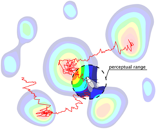
Figure 1. A searcher with a finite perceptual range navigating a heterogeneous landscape using a biased random walk search strategy. In contrast to standard local searchers, which navigate based only on point-wise information, our searcher can use non-local information within its perceptual range to optimize its movement and exploration.

Here we study the role of finite time scales associated with ecological movement and search; specifically, the effect of limited spatial perception when the search time is itself finite. To formalize these aspects, we propose an optimal navigation (ON) model, which allows us to extend the description of search as a biased random walk [11, 14, 24], and reinterpret it in the framework of optimal control theory. The ON model includes a time horizon that quantifies the perceptual range of the searchers along their trajectory and fixes a non-local optimization target for the agents. In the limit of vanishing time horizon (i.e., as the spatial perception shrinks and the information becomes local), the ON model recovers the classic Keller-Segel (KS) drift-diffusion model [25] of local search strategies (i.e., with instantaneous sensing and alignment to the point-wise gradient).

Using simulations and analytical results, we find that a population of non-local searchers moving toward a nutrient patch exhibits distinct transient behavior, clustering faster at the hotspot than local searchers, thereby increasing their search efficiency. Our results show that the maximum efficiency gain occurs when the perceptual range of the searchers matches the environmental length scale over which the nutrient concentration changes significantly. As the search time becomes asymptotically large or small, the efficiency gain from the non-local strategy diminishes, and the searchers behave effectively as local responders. If the environmental length scale changes, we show that the efficiency gain can be maintained as long as searchers can adjust their sensitivity. This means that finite perception remains advantageous to searchers that can rescale their response dynamically, or to populations that contain a diversity of responses. Finally, we consider the effect of interaction between searchers, and show that non-local information consistently reinforces the dominant strategy in the population and leads to improved search efficiency overall, even though multimodality (subpopulations) can appear during the transients. Our framework provides and optimization perspective on a range of collective phenomena in population biology and, more generally, on biologically-inspired search and exploration algorithms, thus shedding light on the role of spatial perception on finite-time search.

2. The classic Keller-Segel model: noisy search with local gradient alignment

A classic model for the dynamics of a population of searchers using local gradient alignment is given by the Keller-Segel equation, which we briefly recap here.

Consider a population of searchers moving in a closed, bounded, d-dimensional domain Ω ⊂ ℝ^d. The searchers move by responding to two concentration fields: to a primary stimulant S₁(x) (e.g., nutrient) with sensitivity χ₁, and to a secondary stimulant S₂(x, t) (e.g., pheromone), released by the agents themselves, with sensitivity χ₂.

On long space and time scales relative to the microscopic motion, one can describe the biased random walk x(t) ∈ Ω of searchers by a Langevin equation [24]:

$\begin{array}{rc}\frac{dx}{dt}=v(x,t)+\sqrt{2D}\xi (t),& (1)\end{array}$

where ξ(t) is a white noise process, D is the coefficient of diffusion, and

$\begin{array}{rc}v(x,t)=\nabla \left({\chi }_1{S}_1(x)+{\chi }_2{S}_2(x,t)\right)& (2)\end{array}$

is the velocity of the searcher. The parameters D, χ₁ and χ₂ are typically inferred experimentally from trajectories of the agents [14, 26], and can sometimes be expressed in terms of microscopic parameters [27]. Note that Equations (1)–(2) describe a searcher that uses local information, since it aligns its velocity instantaneously to the gradients of S₁ and S₂.

The secondary stimulant S₂ introduces interaction between the searchers. If S₂ is assumed to diffuse faster than the searchers, its evolution is given by

$\begin{array}{rc}{S}_2(x,t)={\displaystyle {\int }_{\Omega }}\text{Φ}(x-x^{\prime })\rho (x^{\prime },t)d{x}^{\prime }:=\text{Φ}\ast \rho & (3)\end{array}$

where

$\Phi (x)=\{\begin{array}{l}-\frac{1}{2\pi }\log ||x||\text{for }d=2\hfill \\ \frac{\text{Γ}\left(\frac{d}{2}+1\right)}{d(d-2){\pi }^{d/2}}||x|{|}^{2-d}\text{for }d\ne 2,\hfill & (4)\end{array}$

and Γ is the Gamma function (see Appendix A).

Taking all together, the time evolution of the population density ρ(x, t) of searchers obeying (1)– (3) can be described with a Fokker-Planck equation [28] known as the Keller-Segel (KS) model. In dimensionless variables x → x/L and t → t/T_D, where $T_D=L^2/D$ is the diffusion time of the searchers, the KS equation reads

$\begin{array}{rc}{\partial }_t\rho -{\nabla }^2\rho +{\mathrm{\text{Pe}}}_1\nabla ·(\rho \nabla S_1)+{\mathrm{\text{Pe}}}_2\nabla ·\left(\rho \nabla (\text{Φ}\ast \rho )\right)=0,& (5)\end{array}$

where the parameters Pe₁ = χ₁S_1,av/D and Pe₂ = χ₂S_2,av/D are Péclet numbers quantifying the ratio of diffusive to advective forces on the searchers, and S_1,av, S_2,av are the average stimulant concentrations. Given an initial distribution ρ₀(x): = ρ(x, 0), a stimulant profile S₁(x), and parameters Pe₁ and Pe₂, Equation (5) can be solved numerically using standard techniques. Here, we use a first-order in time, second-order in space forward Euler scheme [29] with upwind discretization and Δx = 0.01 and Δt = 10⁻⁶. We denote the solution of the KS model by ρ_KS(x, t). See Appendix A for a fuller derivation and details of the non-dimensionalization.

2.1. Variational Rewriting of the KS Model

The KS model can be recast in a variational gradient formulation [30, 31]. First, rearrange (5) as an advection equation:

$\begin{array}{rcl}{\partial }_t\rho & +\nabla ·(\rho u)=0& (6)\end{array}$

$\begin{array}{rcl}\mathrm{\text{with }}& u=-\nabla log\rho +v,& (7)\end{array}$

where u is the velocity of the population. Since the velocity of the searchers v is a gradient (2), u is also a gradient:

$\begin{array}{ll}u=\nabla \left(-log\rho +{\mathrm{\text{Pe}}}_1{S}_1+{\mathrm{\text{Pe}}}_2(\text{Φ}\ast \rho )\right).& (8)\end{array}$

All terms in (8) are either local or symmetric with respect to x; hence u can be written [30] as a first variation

$\begin{array}{ll}u=-\nabla \left(\frac{\delta {F}}{\delta \rho }\right),& (9)\end{array}$

where the free energy functional

$\begin{array}{rc}{F}\left[\rho \right]={\displaystyle {\int }_{\Omega }}\left(\rho log\rho -{\mathrm{\text{Pe}}}_1\rho S_1-\frac{{\mathrm{\text{Pe}}}_2}{2}\rho (\text{Φ}\ast \rho )\right)dx& (10)\end{array}$

includes (in order): an entropic term from the stochastic component of the dynamics (2); the internal energy of the stimulant landscape S₁; and a term from the interaction between searchers via the secondary stimulant S₂.

The KS model can then be rewritten in the equivalent gradient flow form

$\begin{array}{rc}{\partial }_t\rho =\nabla ·\left(\rho \nabla \frac{\delta {F}}{\delta \rho }\right),& (11)\end{array}$

which has the important implication that the evolution of ρ(x, t) can be computed using the Jordan-Kinderlehrer-Otto (JKO) variational optimization scheme [31, 32]. From an initial density ρ₀(x), the JKO scheme constructs a sequence of probability distributions {ρ(x, kΔt)}_k≥0

$\begin{array}{rc}\rho (x,(k+1)\Delta t)=arg{\displaystyle \underset{{\rho }^{\prime }}{min}}\left\{\frac{1}{2\Delta t}{d}_W(\rho (x,k\Delta t),{\rho }^{\prime })+{F}\left[{\rho }^{\prime }\right]\right\},& (12)\end{array}$

where Δt > 0 is the time step, and d_W(·, ·) is the Wasserstein distance between two distributions. The solution (12) has been proved to converge to the solution of Equation (5) in the limit Δt → 0 [32].

3. The Optimal Navigation model: a population of searchers with non-local optimization

The variational rewriting (11) and its approximation scheme (12) leads us to formulate the optimal navigation (ON) search model, as follows. Consider a population of searchers that move by performing the optimization (12) over a finite time horizon τ ≥ Δt > 0, which reflects the perceptual range of the agents. Then the time evolution of the population corresponds to a sequence of constrained optimization problems [33], i.e., a succession of JKO solutions, each over time τ.

Starting from the initial density ρ₀(x), we construct the evolution of ρ(x, t), such that each iteration k ≥ 0 finds m(x, s): = ρ(x, kτ + s) for s ∈ [0, τ] by solving the minimization problem:

$\begin{array}{l}\underset{(m,u)}{\text{minimize }}{J}(m,u):={\displaystyle {\int }_0^{\tau }{\displaystyle {\int }_{\Omega }m}}\frac{|u{|}^2}{2}dxds+{F}[m(x,\tau )]\\ \text{ subject to }{\partial }_{s}m+\nabla ·(mu)=0.& (13)\end{array}$

Note that the constraint is the continuity equation ensuring the conservation of ρ as in (6), whereas the cost function ${J}$ contains a transportation cost, which constrains the average motion to geodesics between optimal states, and an end-point term involving the evaluation of the free energy at τ (10). Although we use it here for a particular form of the free energy functional, the formulation is generic: through suitable choice of ${F}$, the ON model (13) converges to a broad class of conservation laws as long as they can be recast as continuity equations and possess a variational structure [30–32, 34].

We denote the solution of the ON model (13) by ρ_ON(x, t; τ), and compute it using Algorithm 1, a gradient descent algorithm inspired by Burger et al. [35] and presented in detail in Appendix B.

Physically, the ON model (13) describes the motion of searchers that optimize their displacement over paths bounded by the time horizon τ. From the proof of the JKO scheme [32], it follows directly that the ON model recovers the local KS model as τ → 0:

$\begin{array}{rc}{\displaystyle \underset{\tau \to 0}{lim}}{\rho }_{\mathrm{\text{ON}}}(x,t;\tau )={\rho }_{\mathrm{\text{KS}}}(x,t)& (14)\end{array}$

For finite horizon τ > 0, the time evolution of the ON model departs from the KS solution due to the effect of non-local information on the movement of the searchers, as explored below.

4. Non-local search: transients and enhanced search efficiency

We use the ON model (13) to study how the finite perception of the agents (encapsulated in the time horizon τ > 0) affects the search at the population level. We first consider non-interacting searchers insensitive to the secreted stimulant, i.e., Pe₂ = 0. The case of interacting searchers is presented in section 6.

Our numerics start with a uniform initial condition ρ₀(x) = 1 and we compute ρ_ON(x, t; τ), the time evolution (13) of the ON population of non-local searchers with time horizon τ > 0. We also compare it to the time evolution (5) of a KS population of local searchers, or equivalently the ON model with τ = 0.

Both the KS and ON models converge to the same stationary solution ρ_∞(x) asymptotically as t → ∞:

$\begin{array}{rcl}{\rho }_{\infty }(x)& :={\displaystyle \underset{t\to \infty }{lim}}{\rho }_{\mathrm{\text{KS}}}(x,t)=\frac{1}{Z}exp\left({\mathrm{\text{Pe}}}_1{S}_1(x)\right)& (15)\end{array}$

$\begin{array}{rc}={\displaystyle \underset{t\to \infty }{lim}}{\rho }_{\mathrm{\text{ON}}}(x,t;\tau ),& (16)\end{array}$

for all τ and S₁, given by the Gibbs-Boltzmann distribution (15), where Z is a normalization constant. This result is well known for the KS equation [28]. To check that ρ_∞(x) is also the stationary solution of the ON model, note that at stationarity $d_W({\rho }_{\infty },{\rho }^{\prime })=0$ in (12), and the result (16) follows from solving for the minimizer.

The approach to stationarity, on the other hand, reveals differences between the KS and ON models. To develop our intuition, let us first consider a linear attractant gradient S₁(x) = αx. Such a landscape is fully characterized by the local gradient ∇S₁(x), and hence non-local searchers have no advantage since τ > 0 provides no further information than what is known by local searchers. In line with this expectation, when we solve the ON model (13) using the method of characteristics (section S2 in the SI), we find that the drift velocity predicted by the KS and ON models coincide for all τ, i.e.,

$u(x,t;\tau )\equiv u(x,t)\mathrm{\text{when }}{S}_1\mathrm{\text{ is linear}}.$

This observation implies that non-local search is only advantageous in landscapes with non-zero curvature. To illustrate this point in more detail, let us consider a static Gaussian concentration of stimulant with characteristic length scale σ ≪ 1 over the domain Ω = [−1/2, 1/2]^d (Figure 2A):

$\begin{array}{rc}{S}_1(x;\sigma )=\frac{1}{\sqrt{{(2\pi )}^d\mathrm{\text{det}}(\Sigma )}}exp\left(-\frac{1}{2}{x}^T{\Sigma }^{-1}x\right),& (17)\end{array}$

where det(·) is the matrix determinant and x^T is the transpose of the vector x. For simplicity of the computations that follow, we take $\Sigma ={\sigma }^2{I}_d$, where I_d is the d-dimensional identity matrix. Such a Gaussian landscape serves as a simple model of a stimulant patch emanating from a point source, and its characteristic length scale σ indicates regions of steep attractant gradients near the source (||x|| ≪ σ) and regions of shallow gradients in the tails of the distribution (||x|| ≫ σ).

FIGURE 2

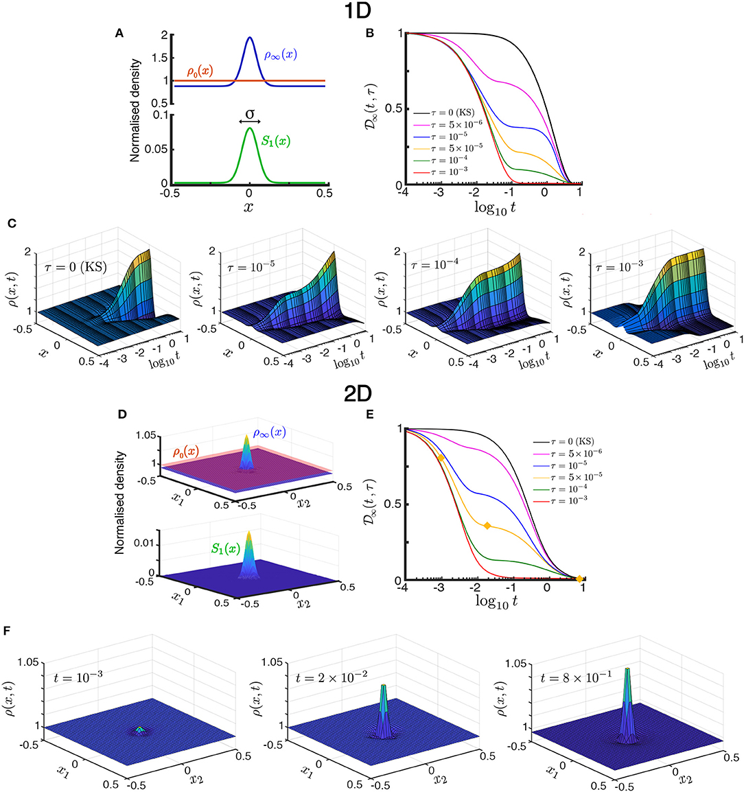
Figure 2. Transient population dynamics in nonlocal search with the ON model in the one-dimensional (A–C) and two-dimensional (D–F) cases. (A) The searchers are initially uniformly distributed with ρ₀(x) = 1. We simulate the time evolution of the population in a Gaussian stimulant profile S₁(x; σ) (17) until they reach the stationary state ρ_∞(x) (15). (B) The approach toward stationarity measured by ${{D}}_{\infty }(t;\tau )$ (18), the normalized L²-distance of the solution to the stationary state. For small time horizons $0<\tau <{\tau }_{\sigma }^{\ast }$, there exists a long-lived intermediate transient state, whereas for $\tau \ge {\tau }_{\sigma }^{\ast }$ the dynamics directly converges to the stationary state as the searchers quickly escape the diffusion-dominated part of the domain. See Figure 3 for the definition of ${\tau }_{\sigma }^{\ast }$. (C) Space-time plots illustrating the convergence toward the stationary state by the ON model in the one-dimensional case (d = 1). The time evolution for increasing time horizon τ = 0, 10⁻⁵, 10⁻⁴, 10⁻³ show qualitatively different transients. The KS model is equivalent to τ = 0. (D,E) are equivalent to (A,B) but for the two-dimensional case. (F) Snapshots of the time evolution of the ON population with time horizon τ = 5 × 10⁻⁵ in the two-dimensional case taken at increasing times [t = 10⁻³, 2 × 10⁻², 8 × 10⁻¹, marked with yellow diamonds in (E)]. The convergence to stationarity displays the two-stage transient: the searchers near the center aggregate during the initial fast transient, whereas the searchers far from the center slowly diffuse toward the center until the stationary state is reached. As the time horizon τ is increased this second slow transient dynamics is reduced. See animations of this solution in the Supplementary Information. All simulations in this figure with Pe₁ = 2 and σ = 0.05.

In Figure 2 we show that, as the time horizon τ is increased, the population of ON searchers exhibits a faster approach to stationarity, as measured by the normalized L²-distance between ρ_ON(x, t; τ) and ρ_∞(x) as a function of time for different values of τ:

$\begin{array}{rc}{{D}}_{\infty }(t;\tau )=\frac{\left|\right|{\rho }_{\mathrm{\text{ON}}}(x,t;\tau )-{\rho }_{\infty }(x)\left|\right|}{\left|\right|{\rho }_0(x)-{\rho }_{\infty }(x)\left|\right|}.& (18)\end{array}$

Figures 2A– C presents the one-dimensional case (d = 1). The effect of the horizon in accelerating the convergence to stationarity is shown in Figure 2B. Note also that for small values of τ, an intermediate, quasi-steady distribution develops during the transient (e.g., τ = 10⁻⁵ in Figures 2B,C). This long-lived intermediate behavior is the result of the population evolving on two timescales [14]: searchers near the maximum of S₁(x) (||x|| ≪ σ) are driven by advection due to the steep gradient, whereas those far from the maximum (||x|| ≫ σ) are driven by diffusion in shallow gradients, and hence move more slowly toward the maximum. Due to the slow diffusive searchers, the stationary state is only reached at a longer time scale t ~ 1. As the horizon τ is increased, this dual behavior (diffusion- or advection-dominated) is lost: the searchers escape quickly the diffusion-dominated part of the domain and, as a result, the distribution approaches stationarity increasingly faster with no appreciable quasi-steady transient distribution (e.g., τ = 10⁻³ in Figures 2B,C). The same behavior is observed also in the two-dimensional case (d = 2) in Figures 2D–F.

Such transient states can be important in biological systems, which typically operate on time scales far from the asymptotic long-time regime [7–9]. In our setting, this situation arises when the search time T (which is analogous to the foraging effort in ecology) is smaller than the diffusion-dominated convergence time, i.e., when T ≪ 1. In such a situation, non-local (ON) searchers have an advantage over local (KS) searchers since they converge faster to areas with high concentration of attractant. To quantify this effect, we consider the amount of stimulant S₁ encountered over the search time T

$\widehat{U}(\tau ,T)={\displaystyle {\int }_0^T{\displaystyle {\int }_{\Omega }{S}_1}}(x){\rho }_{\text{ON}}(x,t;\tau )dxdt,$

and define the relative search efficiency as

$\begin{array}{rc}U(\tau ,T)=\frac{\hat{U}(\tau ,T)}{\hat{U}(0,T)}.& (19)\end{array}$

where $\hat{U}(0,T)$ is the uptake of the population of KS searchers. Therefore, U(τ, T) > 1 indicates a gain in search efficiency, that is, increased stimulant encountered by the population due to the perceptual horizon τ > 0.

Our numerics in Figure 3A show that, given a finite search time T, the search efficiency (19) reaches a maximum $U^{\ast }({\tau }_{\sigma }^{\ast },T)$ for searchers operating with an optimal horizon ${\tau }_{\sigma }^{\ast }$, which depends on the length scale σ for a given dimension d (Figure 3A). The presence of a maximum follows from the asymptotic behavior U(τ, T) → 1 for τ → 0 and τ → ∞. The latter limit follows from the invariance of ρ_∞(x) under τ, and the fact that the integral (19) is asymptotically dominated by the steady state. The presence of a maximum is also observed in the two-dimensional case, but $U^{\ast }({\tau }_{\sigma }^{\ast },T)$ decreases in higher dimensions.

FIGURE 3

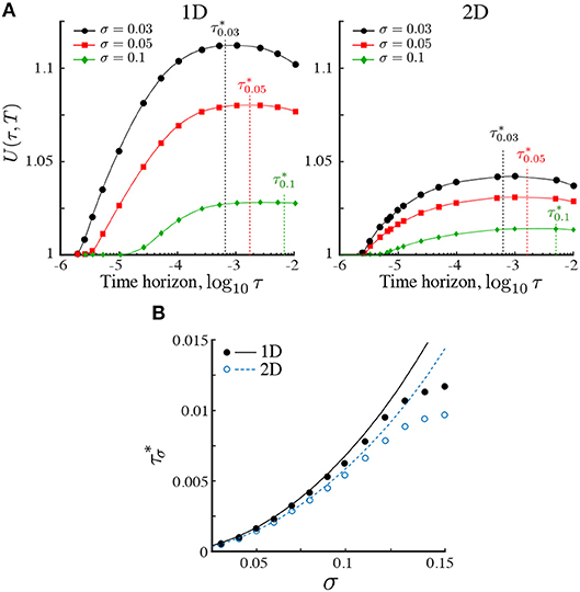
Figure 3. (A) The relative search efficiency (19) of the ON population in one and two dimensions as a function of the time horizon τ for three Gaussian stimulant profiles with length scales σ = 0.03, 0.05, 0.1. All results are computed over a fixed search time T = 10⁻¹. Values of U(τ, T) > 1 indicate improved search efficiency of the ON population as compared to the KS population. The maximum efficiency $U^{\ast }({\tau }_{\sigma }^{\ast },T)$ is achieved at a time horizon ${\tau }_{\sigma }^{\ast }$. For a given Pe₁, the relative search efficiency decreases in higher dimensions due to the increasing dominance of diffusive motion relative to ballistic motion. (B) Comparison of simulations (circles) with our estimate (line) of ${\tau }_{\sigma }^{\ast }$ obtained from (20, 21) by matching the mean-squared distance traveled to the length scale of the landscape as given by Equation (22). The estimate is accurate when σ ≪ 1.

The dependence of ${\tau }_{\sigma }^{\ast }$ with the length scale of the landscape σ obtained numerically from our simulations is shown in Figure 3B with solid (1D) and open (2D) circles. To understand this dependence, consider a searcher at x(t) obeying the Langevin equation (1) under the ON model. The reachable set until t + τ is within a ball of radius x_ms(τ) defined by

$\begin{array}{rc}{x}_{\mathrm{\text{ms}}}^2(\tau )\simeq 2d\tau +{\bar{v}}^2(\tau ){\tau }^2,& (20)\end{array}$

where the two terms represent the displacement due to diffusion and to an effective drift velocity $\bar{v}$ over time τ, respectively. To estimate $\bar{v}(\tau )$, we assume that the search time T is large enough such that individual searchers have explored the whole domain (e.g., for T = 0.1 this is fulfilled when τ > 10⁻³ as seen in Figure 2B). The effective drift velocity can then be approximated by the velocity of an average searcher (over the domain) that maximizes its gain up to time τ,

$\begin{array}{rc}\bar{v}(\tau )\simeq 2{\mathrm{\text{Pe}}}_1{\displaystyle {\int }_{-1/2}^0}\frac{S_1\left(x+x_{\mathrm{\text{ms}}}(\tau )\right)-S_1(x)}{x_{\mathrm{\text{ms}}}(\tau )}dx,& (21)\end{array}$

where the integral is evaluated along a one-dimensional cross-section of the Gaussian landscape

$\begin{array}{l}\overline{v}(\tau )\simeq \frac{2P{e}_1}{x_{ms}(\tau )}{\left(2\pi \sigma \right)}^{-\frac{d}{2}}{{\displaystyle \int }}_{-1/2}^0\left(e^{-\frac{{(x+x_{ms}(\tau ))}^2}{2{\sigma }^2}}-e^{-\frac{x^2}{2{\sigma }^2}}\right)dx\\ =\frac{P{e}_1}{x_{ms}(\tau )}{(2\pi \sigma )}^{-\frac{d-1}{2}}[erf\left(\frac{x_{ms}(\tau )}{\sqrt{2{\sigma }^2}}\right)-erf\left(\frac{1/2}{\sqrt{2{\sigma }^2}}\right)\hfill \\ -erf\left(\frac{x_{ms}(\tau )-1/2}{\sqrt{2{\sigma }^2}}\right)].\hfill \end{array}$

$\begin{array}{}\end{array}$

From (20) and (21), we obtain an estimate of the horizon τ necessary to search over a distance x_ms with the ON model.

The relevance of this estimate is shown in Figure 3B, which shows that for small σ, the maximum search efficiency is attained when the mean-squared displacement of the searchers equals the length scale of the environment:

$\begin{array}{rc}{x}_{\mathrm{\text{ms}}}({\tau }_{\sigma }^{\ast })\simeq \sigma ,& (22)\end{array}$

as obtained with our approximation. The ON model thus predicts that the most efficient searchers are those that tune their horizon such that they traverse the characteristic length scale of the environment within one optimization step. Shorter or longer optimizations lead to a decreased search efficiency.

The dependence of this behavior on the dimension d is also captured by (20), which tells us that the ballistic and diffusive terms balance when $\bar{v}{(\tau )}^2\tau /(2d)$. Thus for a given S₁, τ and Pe₁ the motion of searchers becomes gradually diffusion dominated as the dimension d increases. As a result, the relative search efficiency decreases in higher dimensions as shown in Figure 3.

5. Invariance of search efficiency through rescaling of response sensitivity

The search efficiency of the ON model depends on the length scale σ of the Gaussian landscape: the ON gain diminishes as σ increases (Figure 3). However, as we now show, an ON searcher can retain the same search efficiency under a Gaussian landscape with varying length scale by adjusting Pe₁, its sensitivity to the stimulant.

To see this, consider an ON searcher starting at x₀ exposed to its nutrient micro-environment until time T. The effective gradient for this searcher depends on the starting position x₀ and is given by:

$\begin{array}{rc}{\langle \nabla S_1(x)\rangle }_T=\frac{{\displaystyle {\int }_{x_0}^{x_0+x_{\mathrm{\text{ms}}}(T)}}\left[\frac{S_1\left(x+x_{\mathrm{\text{ms}}}(\tau )\right)-S_1(x)}{x_{\mathrm{\text{ms}}}(\tau )}\right]dx}{x_{\mathrm{\text{ms}}}(T)}.& (23)\end{array}$

For a fixed exploration time T, an increase in the stimulant length scale σ leads to shallower effective gradients (Figure 4A). Using asymptotic techniques, we show in section S1 in the SI that the effective gradient (23) for symmetric Gaussian profiles has a well-defined behavior in the two limiting regimes:

$\{\begin{array}{l}{\langle \nabla S_1(x)\rangle }_T\propto {\sigma }^{-2-d}\text{ as }T\to 0,\hfill \\ {\langle \nabla S_1(x)\rangle }_T\propto {\sigma }^{-d}\text{ as }T\to \infty .\hfill \end{array}(24)$

Together with the form of the dynamics (1), this suggests the following scaling for the Péclet number:

$\begin{array}{rc}{\widetilde{\mathrm{\text{Pe}}}}_1(\sigma ,T)\propto {\sigma }^{\alpha (T,d)},& (25)\end{array}$

with d ≤ α(T, d) ≤ 2 + d.

FIGURE 4

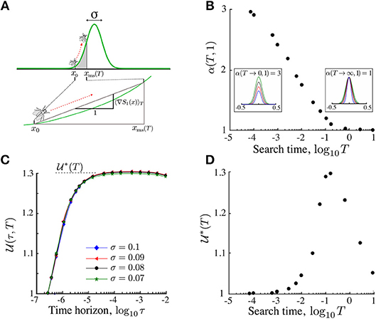
Figure 4. The search efficiency can be made invariant by scaling the sensitivity Pe₁. (A) The displacement of the searcher up to time T is approximated by the displacement in an effective gradient (23). To account for the change in this effective gradient as T or σ varies, we renormalize the Péclet number as in (25). (B) The renormalization yields invariance (26) of the search efficiency under σ (T = 10⁻¹ in this figure). (C) The α(T, d) for d = 1 computed numerically matches the asymptotic results (24): α(T → 0, 1) = 3 and α(T → ∞, 1) = 1. From the perspective of the searcher, the rescaling ${\widetilde{\mathrm{\text{Pe}}}}_1(\sigma ,T)$ is equivalent to renormalizing the landscape. Insets show examples of the renormalized Gaussian landscape with varying σ but the same effective gradient. (D) The optimal renormalized search efficiency ${{U}}^{\ast }(T)$ attainable by adapted agents achieves a maximum at search time T∗~ 0.1. Hence non-local search is maximally advantageous for foraging times much smaller than the diffusion time T_D = 1.

We have tested this scaling by obtaining the ON solution (13) over a given T for Gaussian profiles with different σ using the renormalized Péclet number (25). We then compute the relative search efficiency (19) for this solution, $U(\tau ,T;{\widetilde{\mathrm{\text{Pe}}}}_1(\sigma ,T))$. Our numerics in Figure 4B show that the search efficiency curves for the renormalized parameter (25) for different σ collapse on a single curve:

$\begin{array}{rc}U(\tau ,T;{\widetilde{\mathrm{\text{Pe}}}}_1(\sigma ,T))\approx {U}(\tau ,T).& (26)\end{array}$

The exponent α(T, 1), i.e., for d = 1, is obtained numerically (Figure 4C) is consistent with the expected asymptotic limits (24). Note that, the effective gradient (23) is a function of x_ms(τ), which changes with dimension. Therefore, although for any d a scaling relationship exists, it will be different from the curve in Figure 4C depending on d.

Hence the search efficiency can be made invariant for different environmental length scales σ by rescaling the Péclet number (25). Alternatively, adjusting α(T, d) can be viewed as responding to a “renormalized landscape” $\left[{\widetilde{\mathrm{\text{Pe}}}}_1{S}_1(x)\right]$ in order to maintain the ON search efficiency. This is intuitive in limiting cases: when the search time is small (T → 0), the efficiency remains unchanged on landscapes with similar local gradients near the center (x₀ ≪ 1); when the search time is large (T → ∞), the efficiency is invariant for landscapes with similar effective gradient over the whole domain (see inset of Figure 4C).

This result suggests that searchers can optimize their search efficiency by adjusting their response sensitivity [as in the scaling (25)] so as to balance the relative effect of the advection and diffusion velocities or, in other words, the relative importance of gradient optimization vs. noisy exploration. Since the diffusion coefficient D is typically independent of S₁(x) [27], the adjustment of Pe₁ could be achieved by varying the sensitivity as a function of the stimulant, i.e., χ₁(S₁(x)) (see Appendix A). In the Discussion, we explain possible biological mechanisms to achieve this effect.

Is non-local search advantageous over search times relevant for ecological systems? The invariant search efficiency ${U}(\tau ,T)$ characterizes the performance of a searcher that is tuned to the intrinsic length scale of the stimulant landscape during its search time T. In Figure 4D, we show the dependence of the maximum renormalized search efficiency (26) with the search time T. As expected, for short search time T → 0 and long search time T → ∞, the efficiency ${{U}}^{\ast }(T)$ is equivalent to the local search strategy, i.e., ${{U}}^{\ast }(T)\to 1$. However, between both extremes, searchers benefit from finite perception. Our numerics show that the optimal search time is $T^{\ast }=argmax{{U}}^{\ast }(T,{\tau }^{\ast })~0.1<1=T_D$. Hence finite perception is maximally advantageous for search times smaller than the diffusion time, a fact that is typical in ecological systems (section 7).

6. Agent interaction in the Optimal Navigation model: increased efficiency and multimodality

Until now, we have considered a population of non-interacting searchers reacting only to an external stimulant S₁(x). Now we consider searchers which also interact with each other through an attractive secondary stimulant S₂(x, t) (i.e., Pe₂ > 0). The effect of such interaction can be potentially contradictory: agent interaction may increase aggregation; however, aggregation might not increase search efficiency for the population if a large proportion of the agents clumps away from the stimulant source if the sensitivity to stimulant S₂ becomes larger.

To explore these effects numerically, we use the ON model (13) with a weak interaction in the free energy (10)

$\begin{array}{rc}{\mathrm{\text{Pe}}}_2=\beta {\mathrm{\text{Pe}}}_1,\beta \ll 1& (27)\end{array}$

and compute the time evolution of the population for various β and τ. We restrict ourselves to the weak interaction case (β ≪ 1) to facilitate our numerics. Specifically, to prevent infinite density concentration at finite time, a well-known artifact of the KS model, by applying a small regularizing factor ωρ² with 0 < ω ≪ 1 to the free energy ${F}\left[\rho \right]$ (10). This is a volume exclusion term that models the fact that agents occupy a finite volume in space [36, 37] [see (B5) in Appendix B]. The weak interaction assumption (β ≪ 1) is important for numerical performance so as to avoid high velocities near the concentration point that would necessitate a finer time discretization to maintain the CFL condition (see Appendix B).

A summary of the numerics of the two-dimensional ON case with different horizons τ and levels of interaction β over different search times T is presented in Figure 5. In all cases, the presence of interaction reduces the tails of the population density and increases aggregation near the maximum of S₁ at the center of the domain. This becomes more noticeable as the search time grows and we approach stationarity (Figure 5, right column). During transients, however, agent interaction induces multimodality in the population (Figure 5, left and middle column). This implies that some searchers move away from the maximum of the stimulant S₁(x) and aggregate into transient subpopulations. This behavior arises due to the non-linear response of the searchers to the gradient of S₁(x): for steep gradients of S₁(x), agents are driven by attraction to S₁, whereas for shallow gradients of S₁(x) the agents are driven by the interaction with the rest of the population through the secreted stimulant S₂. In contrast, for non-interacting agents (β = 0) the distribution is always uni-modal (Figure 5).

FIGURE 5

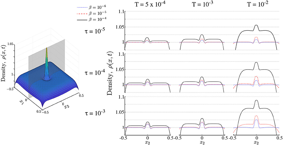
Figure 5. Populations of interacting ON agents. Right panel shows snapshots of a population of ON searchers along the cutting plane shown in gray on the left hand panel. Snapshots are shown with time horizons τ and interaction strength β for different search times T. Interaction increases aggregation at the maximum of the nutrient profile (the center of the domain) and reduces the long tails leading to the emergence of multimodality. Simulations performed with Pe₁ = 2, σ = 0.05.

Figure 6 shows the dependence of multimodality on T and τ at three different interaction strengths β = 5 × 10⁻⁵, 10⁻⁵, 5 × 10⁻⁶. We find that interaction introduces multimodality, as part of the population clumps away from the source of the attractant. For higher interaction strength (β = 5 × 10⁻⁵) multimodality is only present during early transients, and is independent of the time horizon τ, since the strongly interacting population rapidly converges to the peak of the primary stimulant. As the interaction strength β decreases, multimodality lasts longer, but it decreases as the time horizon τ increases. This is in line with the expectation that increased spatial perception τ or search time T leads to overlapping information of the searchers about the environment, whereas, in contrast, when τ and/or T are small, the searchers remain isolated within their local environment, thus leading to multimodality by local aggregation. As the interaction decreases further multimodality disappears.

FIGURE 6

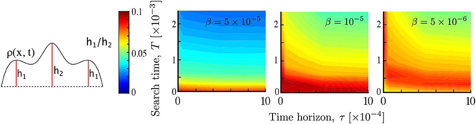
Figure 6. Multimodality as a result of agent interaction. The relative prominence of the smaller modes h₁/h₂ is computed for different parameters T, τ and β. As the interaction β decreases, multimodality gradually shifts to longer times and its magnitude also depends on the time horizon. This results from non-local searchers reaching more quickly a unimodal aggregate at the stimulant source. Simulations performed with Pe₁ = 2, σ = 0.05.

Importantly, despite the presence of such mildly multimodal transients with clumped subpopulations, agent interaction β leads to an overall improvement in the search efficiency U∗(τ∗, T) at a shorter time horizon τ∗ (Figure 7). This behavior follows from the increased concentration of searchers around the center (on average), and suggest that when resources are sparsely distributed, agent interaction in conjunction with a finite perceptual range, could play a role in improving the collective sensing of the environment toward improved population efficiency.

FIGURE 7

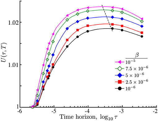
Figure 7. Relative search efficiency (19) of an ON population of interacting agents against time horizon with different interaction strengths β. As β grows, the search efficiency increases and the maximum is attained at smaller time horizons (dashed line). The improvement in the search efficiency with interaction follows from the increased accumulation of agents at the maximum of the nutrient and the reduced long tails far from the center of the domain (Figure 5). Simulation parameters: ${\mathrm{\text{Pe}}}_1=2,\sigma =0.05,T=5\times 10^{-2}$.

7. Discussion

In this work, we studied how finite perception influences the dynamics and efficiency of collective random search in a population of agents. Using concepts from optimal control and random walks, we proposed a model that encapsulates the spatial information the searchers possess as a time horizon for an optimization problem. Simulations of the dynamics of population search show that non-local information affects the movement strategy, as compared with the standard Keller-Segel model based on local optimization. Although non-local search does not change the stationary state, it leads to qualitatively different transient responses of possible relevance in biological systems [7]. For example, marine bacteria have been observed to aggregate at food patches much faster (~ 10¹− 10² s) [38, 39] than the timescale to reach the steady state distribution ($T_D~10^4-10^5$ s, based on D ~ 10²−10³μm²/s [40] and typical inter-patch distance L ~ 10³μm [41]). Similarly, in several rodent species diffusion coefficients of D ~ 200 m²/day and home range of L ~ 70 m have been reported [42]. Therefore, the time it takes to reach home by diffusion (~ 25 days) is much longer than their typical response time (~ 1 day).

We find that non-local information can account for the increase in the search efficiency under transient search times: the maximum efficiency is reached when the mean-squared displacement of the searchers matches the environmental length scale of the stimulant. When the time horizon vanishes or when the search time is infinite, our model recovers the response of local searchers. This is in accordance with the fact that when long-range cues are unreliable, local response leads to highest efficiency [15].

We also showed that the search efficiency can be made invariant to changes in environmental length scales by suitably scaling the response sensitivity. As a consequence, a searcher with a given perceptual range may always achieve its maximum efficiency by dynamically adjusting its sensitivity to the environmental stimuli. This can be achieved either by dynamically rescaling the responses via adaptation at the agent level [43], or by the presence of a distribution of sensitivities among the agents at the population level. For example, it has been shown that phenotypic heterogeneity (or plasticity) across a population can be used to achieve maximum search efficiency in patchy environments [44].

Finally, we considered the effect of interaction between searchers with finite perception and showed that interaction can lead to unimodal or multimodal population distributions on transient timescales. Multimodality appears even in the presence of unimodal stimulant landscapes due to a trade-off between following the environmental gradient or the rest of the population. In our numerics, interaction always improved the overall search efficiency of the population.

Recent theoretical and experimental studies [45, 46] also suggest that rodents (and other higher animals) store spatial information of their environment, and in doing so commonly prefer longer (non-trivial) future paths as opposed to paths leading to immediate rewards. These results are in line with a predictive optimization based on spatial knowledge, as in the ON model, where the searcher weighs up local cues with those at a distance to inform the planning of the future trajectory as opposed to an immediate (gradient) optimization. Clearly, the perceptual horizon in the ON model is a very coarse abstraction of the spatial information the organism perceives (for example in its visual field) or is encoded in its neural or cellular memory. Going beyond our framework would require explicit assumptions about the sensory or cognitive mechanisms involved in search and navigation, an area of interesting future research which is out of the scope of this work.

Our work opens up several directions of research. Beyond our simple setup, it would be of interest to study search on temporally-fluctuating or patchy nutrient landscapes [47] using non-local strategies. Random search theory based on local response predicts that when a searcher is positioned equally far from two nutrient patches it is equally likely to explore either patch. However, on transient timescales, nonlocal searchers are expected to explore the patch with denser resources with higher probability. This direction will be the object of future work.

Data Availability

Movies accompanying Figure 2F and a Matlab implementation of the ON model in 1D and 2D is available at: https://doi.org/10.6084/m9.figshare.7477568.v1.

Author Contributions

AG and MB conceived and developed the study. AG performed the research under the supervision of MB and JC. AG and MB wrote the manuscript, with inputs from JC.

Conflict of Interest Statement

The authors declare that the research was conducted in the absence of any commercial or financial relationships that could be construed as a potential conflict of interest.

Acknowledgments

AG acknowledges funding through a PhD studentship under the BBSRC DTP at Imperial College (BB/M011178/1). JC acknowledges funding from the EPSRC EP/P031587/1. MB acknowledges funding from the EPSRC (EP/N014529/1 and EP/I032223/1).

Supplementary Material

The Supplementary Material for this article can be found online at: https://www.frontiersin.org/articles/10.3389/fphy.2018.00153/full#supplementary-material

References

1. Hein AM, Carrara F, Brumley DR, Stocker R, Levin SA. Natural search algorithms as a bridge between organisms, evolution, and ecology. Proc Natl Acad Sci USA. (2016) 113:9413–20. doi: 10.1073/pnas.1606195113

PubMed Abstract | CrossRef Full Text | Google Scholar

2. Bell WJ. Searching Behaviour. The Behavioural Ecology of Finding Resources. Dordrecht: Springer (2012).

Google Scholar

3. Viswanathan GM, da Luz MGE, Raposo EP, Stanley HE. The Physics of Foraging. An Introduction to Random Searches and Biological Encounters. Cambridge: Cambridge University Press (2011).

Google Scholar

4. Stephens DW, Krebs JR. Foraging Theory. New Jersey, NJ: Princeton University Press (1986).

Google Scholar

5. MacArthur RH, Pianca ER. On optimal use of a patchy environment. Am Nat. (1966) 100:603–9.

Google Scholar

6. Charnov EL. Optimal foraging, the marginal value theorem. Theor Popul Biol. (1976) 9:129–36.

PubMed Abstract | Google Scholar

7. Hastings A. Transients: the key to long-term ecological understanding? Trends Ecol Evol. (2003) 19:39–45. doi: 10.1016/j.tree.2003.09.007

PubMed Abstract | CrossRef Full Text | Google Scholar

8. Strelkowa N, Barahona M. Switchable genetic oscillator operating in quasi-stable mode. J R Soc Interface. (2010) 7:1071–82. doi: 10.1098/rsif.2009.0487

PubMed Abstract | CrossRef Full Text | Google Scholar

9. Strelkowa N, Barahona M. Transient dynamics around unstable periodic orbits in the generalized repressilator model. Chaos (2011) 21:023104. doi: 10.1063/1.3574387

PubMed Abstract | CrossRef Full Text | Google Scholar

10. Schrödinger E. What is Life?: With Mind and Matter and Autobiographical Sketches. Cambridge: Cambridge University Press (1992).

Google Scholar

11. Berg HC. Random Walks in Biology. Princeton University Press (1993).

Google Scholar

12. Bénichou O, Coppey M, Moreau M, Suet PH, Voituriez R. Optimal search strategies for hidden targets. Phys Rev Lett. (2005) 94:198101. doi: 10.1103/PhysRevLett.94.198101

PubMed Abstract | CrossRef Full Text | Google Scholar

13. Tejedor V, Voituriez R, Bénichou O. Optimizing persistent random Searches. Phys Rev Lett. (2012) 108:088103. doi: 10.1103/PhysRevLett.108.088103

PubMed Abstract | CrossRef Full Text | Google Scholar

14. Okubo A, Levin SA. Diffusion and Ecological Problems: Modern Perspectives. New York, NY: Springer-Verlag (2001).

Google Scholar

15. Vergassola M, Villermaux E, Shraiman BI. 'Infotaxis' as a strategy for searching without gradients. Nature. (2007) 445:406–9. doi: 10.1038/nature05464

PubMed Abstract | CrossRef Full Text | Google Scholar

16. Bartumeus F, Catalan J. Optimal search behavior and classic foraging theory. J Phys A Math Theor. (2009) 42:434002. doi: 10.1088/1751-8113/42/43/434002

CrossRef Full Text | Google Scholar

17. Viswanathan GM, Buldyrev SV, Havlin S, da Luz MGE, Raposo EP, Stanley HE. Optimizing the success of random searches. Nature 401:911.

PubMed Abstract

18. Moser EI, Kropff E, Moser MB. Place cells, grid cells, and the brain's spatial representation system. Annu Rev Neurosci. (2008) 31:69–89. doi: 10.1146/annurev.neuro.31.061307.090723

PubMed Abstract | CrossRef Full Text | Google Scholar

19. Mistro DC, Rodrigues LAD, Ferreira WC. The Africanized honey bee dispersal: a mathematical zoom. Bull Math Biol. (2005) 67:281–312. doi: 10.1016/j.bulm.2004.07.006

PubMed Abstract | CrossRef Full Text | Google Scholar

20. Gomez-Marin A, Stephens GJ, Louis M. Active sampling and decision making in Drosophila chemotaxis. Nat Commun. (2011) 2:441. doi: 10.1038/ncomms1455

PubMed Abstract | CrossRef Full Text | Google Scholar

21. Mitchell A, Romano GH, Groisman B, Yona A, Dekel E, Kupiec M, et al. Adaptive prediction of environmental changes by microorganisms. Nature (2009) 460:220–4. doi: 10.1038/nature08112

PubMed Abstract | CrossRef Full Text | Google Scholar

22. van den Bos R. Animal anticipation: a perspective. In: Poli R, editor. Handbook of Anticipation: Theoretical and Applied Aspects of the Use of Future in Decision Making. Cham: Springer (2017). pp. 1–13.

Google Scholar

23. Gosztolai A, Schumacher J, Behrends V, Bundy JG, Heydenreich F, Bennett MH, et al. GlnK Facilitates the dynamic regulation of bacterial nitrogen assimilation. Biophys J. (2017) 112:2219–30. doi: 10.1016/j.bpj.2017.04.012

PubMed Abstract | CrossRef Full Text | Google Scholar

24. Codling EA, Plank MJ, Benhamou S. Random walk models in biology. J R Soc Interface. (2008) 5:813–34. doi: 10.1098/rsif.2008.0014

PubMed Abstract | CrossRef Full Text | Google Scholar

25. Keller EF, Segel LA. Initiation of slime mold aggregation viewed as an instability. J Theor Biol. (1970) 26:399–415. doi: 10.1016/0022-5193(70)90092-5

PubMed Abstract | CrossRef Full Text | Google Scholar

26. Boyer D, Dean DS, Mejía-Monasterio C, Oshanin G. Optimal estimates of the diffusion coefficient of a single Brownian trajectory. Phys Rev E. (2012) 85:031136. doi: 10.1103/PhysRevE.85.031136

PubMed Abstract | CrossRef Full Text | Google Scholar

27. Othmer HG, Dunbar SR, Alt W. Models of dispersal in biological systems. J Math Biol. (1988) 26:263–98. doi: 10.1007/BF00277392

PubMed Abstract | CrossRef Full Text | Google Scholar

28. Gardiner C. Stochastic Methods. Berlin: Springer (2009).

PubMed Abstract | Google Scholar

29. Carrillo JA, Chertock A, Huang Y. A finite-volume method for nonlinear nonlocal equations with a gradient flow structure. Commun Comput Phys. (2015) 17:233–58. doi: 10.4208/cicp.160214.010814a

CrossRef Full Text | Google Scholar

30. Carrillo JA, McCann RJ, Villani C. Kinetic equilibration rates for granular media and related equations: entropy dissipation and mass transportation estimates. Rev Mat Iberoamericana. (2003) 19:971–1018. Available online at: https://projecteuclid.org/euclid.rmi/1077293812

Google Scholar

31. Jordan R, Kinderlehrer D, Otto F. The variational formulation of the Fokker–Planck equation. SIAM J Math Anal. (1998) 29:1–17. doi.: 10.1137/S0036141096303359

Google Scholar

32. Blanchet A, Calvez V, Carrillo JA. Convergence of the mass-transport steepest descent scheme for the subcritical Patlak-Keller-Segel model. SIAM J Numer Anal. (2008) 46:691–721. doi: 10.1137/070683337

CrossRef Full Text | Google Scholar

33. Benamou JD, Brenier Y. A computational fluid mechanics solution to the Monge-Kantorovich mass transfer problem. Numer Math. (2000) 84:375–93. doi: 10.1007/s002110050002

CrossRef Full Text | Google Scholar

34. Carrillo JA, Moll JS. Numerical simulation of diffusive and aggregation phenomena in nonlinear continuity equations by evolving diffeomorphisms. SIAM J Sci Comput. (2009) 31:4305–29. doi: 10.1137/080739574

CrossRef Full Text | Google Scholar

35. Burger M, Franek M, Schönlieb CB. Regularized regression and density estimation based on optimal transport. Appl Math Res Express. (2012) 2012:209–53. doi: 10.1093/amrx/abs007

CrossRef Full Text | Google Scholar

36. Calvez V, Carrillo JA. Volume effects in the Keller-Segel model: energy estimates preventing blow-up. J Math Pures Appl. (2006) 86:155–75. doi: 10.1016/j.matpur.2006.04.002

CrossRef Full Text | Google Scholar

37. Carrillo JA, Hittmeir S, Jängel A. Cross diffusion and nonlinear diffusion preventing blow up in the Keller-Segel model. Math Models Methods Appl Sci. (2012) 22:1250041. doi: 10.1142/S0218202512500418

CrossRef Full Text | Google Scholar

38. Blackburn N, Fenchel T, Mitchell J. Microscale nutrient patches in planktonic habitats shown by chemotactic bacteria. Science (1998) 282:2254–6. doi: 10.1126/science.282.5397.2254

PubMed Abstract | CrossRef Full Text | Google Scholar

39. Seymour JR, Simó R, Ahmed T, Stocker R. Chemoattraction to dimethylsulfoniopropionate throughout the marine microbial food web. Science. (2010) 329:342–5. doi: 10.1126/science.1188418

PubMed Abstract | CrossRef Full Text | Google Scholar

40. Kiørboe T, Grossart HP, Ploug H, Tang K. Mechanisms and rates of bacterial colonization of sinking aggregates. Appl Environ Microbiol. (2002) 68:3996–4006.

PubMed Abstract | Google Scholar

41. Azam F, Ammerman JW. Cycling of organic matter by bacterioplankton in pelagic maring ecosystems: microenvironmental considerations. In: Holm-Hansen O, Bolis L, Gilles R, editors. Marine Phytoplankton and Productivity. Berlin: Springer (1984).

Google Scholar

42. Giuggioli L, Abramson G, Kenkre VM, Suzán G, Marcé E, Yates TL. Diffusion and home range parameters from rodent population measurements in Panama. Bull Math Biol. (2005) 67:1135. doi: 10.1016/j.bulm.2005.01.003

PubMed Abstract | CrossRef Full Text | Google Scholar

43. Lazova MD, Ahmed T, Bellomo D, Stocker R, Shimizu TS. Response rescaling in bacterial chemotaxis. Proc Natl Acad Sci USA. (2011) 108:13870–5. doi: 10.1073/pnas.1108608108

PubMed Abstract | CrossRef Full Text | Google Scholar

44. Hollander J, Verzijden M, Svensson E, Brönmark C. Dispersal and phenotypic plasticity. In: Hansson LA, Akesson S, editors. Animal Movement Across Scales. Oxford: Oxford University Press (2014). pp. 110–125.

Google Scholar

45. Mattar MG, Daw ND. Prioritized memory access explains planning and hippocampal replay. Nat Neurosci. (2018) 21:1609–17. doi: 10.1038/s41593-018-0232-z

PubMed Abstract | CrossRef Full Text | Google Scholar

46. Pfeiffer BE, Foster DJ. Hippocampal place-cell sequences depict future paths to remembered goals. Nature (2013) 497:74–9.

PubMed Abstract | Google Scholar

47. Chupeau M, Bénichou O, Redner S. Search in patchy media: exploitationexploration tradeoff. Phys Rev E. (2017) 95:012157. doi: 10.1103/PhysRevE.95.012157

PubMed Abstract | CrossRef Full Text | Google Scholar