Influence of Resonant Absorption on the Generation of the Kelvin-Helmholtz Instability

1. Introduction

The solar corona is continuously disturbed by perturbations at photospheric and chromospheric levels, either locally by means of e.g., convective motions or reconnection, or globally, by means of the internal oscillations of the Sun leaking radially outwards (and particularly p-modes). These continuous perturbations generate stress in the magnetic field and energy release processes lead to upflow of material that fills the coronal magnetic field with plasma, thereby generating coronal loops.

The particulars of coronal loop generation and destruction is, however, still a matter of debate. Observations mostly show the cooling stage of coronal loops [1], in which loops appear and disappear in specific bandpasses a time that can be either large or small [2], depending on the radiative cooling time and also on the unresolved substructure of loops [3–5]. Loops are thought to be composed of elementary substructures called strands. These strands may be elementary in the magnetic sense, being associated with tiny concentrations of magnetic field in the photosphere (of a few 100 km in width, e.g., [6]), or may be elementary in the sense of their independent thermodynamic evolution due to the fact that transport coefficients in the corona, and thus most plasma processes, are field aligned. On the other hand, the heating stage of the strands forming a loop is still unresolved, and are thought to occur in very short time and on very small spatial scales. Estimations of loop widths in the corona are thus based on the observed widths during the process of cooling, assuming that neighboring field lines composing the loop evolve more or less similarly. Even though there is a debate on how many strands actually compose a coronal loop on average [7], there seems to be consensus over the observed width of coronal loops (or the envelope of the strand bundle). Indeed, observations in coronal lines indicate an average coronal loop width of roughly 2 Mm [4, 8, 9], confirmed also at higher resolution by the characteristic width of coherent catastrophic cooling of loops [10, 11].

Besides the substructure of loops, other very relevant questions in coronal loop dynamics are how large are their boundary layers and what actually defines them [12–14]. The relevance lies particularly in the field of MHD waves. Kink waves (a particular class of transverse MHD waves characterized by the transverse displacement of the entire waveguide, [15, 16]) have been shown to permeate the corona and may be a candidate to heat the corona [17–20]. An observational characteristic of these waves is their fast damping and the leading theory explaining the damping is resonant absorption [21–26], also known as mode coupling in the case of propagating modes, contrary to standing modes [27–31]. During this process the plasma motions involved in the kink mode vary, and pass from initially being coherent lateral displacements of the loop's axis (thus affecting the whole loop) to azimuthal displacements highly localized in the regions within the loop where the resonance occurs. This happens where the kink speed matches the local Alfvén speed (or, in the case of driven propagating modes, where the kink frequency matches the local Alfvén frequency). These locations are usually assumed to be primarily at the edges of loops, although non-uniform loop distributions with resonance locations within the loop evolve similarly due to the collective nature of the kink mode [32, 33].

The formation process of coronal loops is very likely 3D, involving the local magnetic field topology and the conversion of the magnetic free energy into kinetic and thermal energies. This means that the initial energy deposition can have a characteristic area across the field over which magnetic field lines are affected roughly equally. This is the case for instance either through magnetic reconnection (case in which the field lines reconnect along separatrices) or through waves (case in which the diffusion process is linked to the 3D nature of the wave). This argument therefore poses a big question on how is the boundary layer of a coronal loop characterized. If the heating process is very spatially localized (which may be more the case of magnetic reconnection) it may suggest that the subsequent upflow into the loop from chromospheric evaporation is equally highly localized and therefore that the boundary layer separating the loop with the external medium is very thin [12]. If, however, the heating process has a smooth spatial distribution (for instance in the case of a wave produced by convective motions, which are usually coherent over some area) the width of the loop should be broader from the beginning.

The thinner the boundary layer, the more concentrated the azimuthal motions from resonant absorption will be [34] and therefore the larger the velocity shear produced with the surroundings. This velocity shear is additional to the velocity shear that is naturally produced by the (global) lateral displacement from the kink mode [35]. This velocity shear from the global motion happens between the internal motion of the loop and the (dipole-like) motion of the external plasma (produced by the displacement of the loop). On the other hand, it has been speculated that the resonance increases the shear with the external (dipole-like) motion due to the increase in amplitude in the azimuthal motions around the loop edge that the resonance entails [36]. Additionally, the resonance also produces an internal velocity shear between the inner shells of the loop due to phase mixing [37]. For these reasons it has been assumed that resonant absorption enhances the generation of dynamic instabilities due to shear flows [38]. In this paper, we study the effects of these additional shearing layers from the resonance and assess their influence on the generation of dynamic instabilities, and in particular the Kelvin-Helmholtz instability.

Transverse wave-induced Kelvin-Helmholtz rolls (also known as TWIKH rolls) are expected to exist from a large amount of recent numerical simulations in coronal conditions [36, 39–41], and also in prominences [38] and spicules [42]. Although TWIKH rolls have still not been observed directly due to the lack of instrumental resolution [43], there are a number of indirect observational characteristics that seem to match current spectroscopic and imaging observations, such as the generation of strand-like structure [36], the observed 3D motion of prominence strands combined with heating [38, 44], the differential emission measure broadening of loops [45] or the corrugated Doppler shift transitions across spicules [42]. Karampelas and Van Doorsselaere [46] have shown that the continuous driving of kink waves in loops leads to fully turbulent loops due to the TWIKH rolls. The potential existence of TWIKH rolls is particularly interesting for coronal heating since it provides a means to the waves to dissipate their energy [47]. Indeed, the generated turbulent-like regime of vortices and current sheets in the TWIKH rolls leads to additional wave dissipation [38, 41].

TWIKH rolls differ from the more generally known velocity shear-induced KHI vortices [48–51] in that the velocity shear is not laminar, constant and field-aligned, but oscillatory and at an angle to the magnetic field (perpendicular in the case of non-twisted flux tubes). The non-zero angle of the wave vector with the magnetic field implies a lower magnetic tension opposing the development of the instability. [52, 53] have analytically shown that this constitutes a major difference leading to flux tubes being always K-H unstable to such flow, regardless of the amount of twist. This finding supports previous numerical results of TWIKH rolls produced by very low amplitude kink modes [36].

The article is organized as follows. We introduce the numerical model in section 2, together with the initial conditions, MHD equations and details of the code. In section 3 we present the results, which we discuss in section 4 and conclude the paper.

2. Numerical Model

2.1. Initial Conditions

The numerical model consists of a straight, cylindrical flux tube (with circular cross-section) in pressure equilibrium with the background, representing a coronal loop. Our experiments (and the results we obtain) are largely independent of the conditions within the flux tube and the corresponding contrast with the ambient corona. This is because the specifics of the KHI are relatively insensitive to the density and magnetic field contrast, compared to the velocity shear, boundary layer thickness and loop radius to length ratio. For instance, uniform temperature or uniform magnetic field (hence, a cool or hot loop) would lead to the same results [43]. The presence of magnetic twist in the loop delays the onset of the KHI [51, 54, 55] but does not suppress it [52].

As observed in some loops [25], here we choose loops that are all hotter and denser than the background by a factor of 3, i.e., T_i/T_e = 3 and ρ_i/ρ_e = 3. Correspondingly, the loop-aligned magnetic field is slightly lower than the background field to keep pressure balance. We set the external temperature and total number density to $T_e=10^6$K and $n_e=10^9$ cm⁻³, respectively. The external and internal magnetic fields are B_e = 18.63 G and B_i = 17.87 G, respectively. The plasma β parameter outside and inside the flux tube is equal to 0.01 and 0.098, respectively.

We consider different cases of loops with and without boundary layer. This layer connects the internal and external plasma and is described as follows:

$\begin{array}{ll}\rho (x,y)={\rho }_e+({\rho }_i-{\rho }_e)\zeta (x,y),& (1)\end{array}$

where

$\begin{array}{ll}\zeta (x,y)=\frac{1}{2}\left(1-tanh\left(b\left(r(x,y)-\frac{1}{2}\right)\right)\right).& (2)\end{array}$

Here, (x, y) denotes the plane perpendicular to the loop axis (along z). The $r(x,y)=\sqrt{(}{x}^2+y^2)/w$ term denotes the normalized distance from the loop center and w = 2 Mm denotes the loop width (diameter). We take the case of a loop with b = 0.01, which essentially describes a step function between internal and external plasma (and therefore no boundary layer), and a second case with b = 16, leading to a boundary layer width of 0.4 R, with R = 1 Mm, the radius of the loop.

At t = 0 a transverse perturbation in x aimed at triggering mainly the fundamental kink mode is set by imposing a velocity perturbation along the loop that has the same spatial distribution of the density. That is, we have v_x = v₀ sin(zπ/L)ζ(x, y), where z denotes the distance along the loop, L = 200 Mm, and v₀ = 16.6 km s⁻¹. Given that the internal Alfvén speed is v_{A, i} = 1006 km s⁻¹, the initial amplitude A relative to internal Alfvén speed corresponds to A/v_{A, i} = 0.0165, and can therefore be considered nonlinear, since, as defined by Ruderman and Goossens [56], the non-linearity parameter $\nu \approx \frac{AL}{R}=3.3$ is larger than 1. This velocity is chosen to mimic usually observed kink mode amplitudes (most of the energy of the initial perturbation leaks out, and the average velocity in the first quarter oscillation is equal to ≈ 9 km s⁻¹). Following the perturbation, the loop oscillates with a standing kink mode with a period of P ≈ 315 s, approximately equal to the expected period, given that the kink speed is c_k = 1256 km s⁻¹. It is worth mentioning that this numerical model corresponds to the impulsively excited loop model used in Van Doorsselaere et al. [45].

The choice of no boundary layer initially for one of our flux tube cases has a 2-fold motivation. As explained in the introduction, it is not unreasonable to think that when a loop first forms, presumably by an impulsive heating event somewhere along the loop, if the heating is very localized in space it may trigger very localized chromospheric evaporation, thereby producing a sharp boundary layer. The second reason behind this choice has to do with the late onset of resonant absorption, a time delay that allows to investigate more properly the role it has on the KHI.

2.2. MHD Equations and Numerical Scheme

We solve the following set of resistive MHD equations without gravity:

$\begin{array}{ll}\frac{\partial \rho }{\partial t}+\nabla ·(\rho \overrightarrow{v})=0,& (3)\end{array}$

$\begin{array}{ll}\frac{\partial }{\partial t}(\rho \overrightarrow{v})+\nabla ·\left[\rho \overrightarrow{v}\overrightarrow{v}+\left(p+\frac{{\overrightarrow{B}}^2}{8\pi }\right)\overrightarrow{I}-\frac{\overrightarrow{B}\overrightarrow{B}}{4\pi }\right]=0,& (4)\end{array}$

$\begin{array}{ll}\frac{\partial \overrightarrow{B}}{\partial t}+\nabla \times \left(\frac{\eta }{\mu }\overrightarrow{j}-\overrightarrow{v}\times \overrightarrow{B}\right)=0,& (5)\end{array}$

$\begin{array}{l}\frac{\partial }{\partial t}\left(\frac{p}{\gamma -1}+\frac{1}{2}\rho {\overrightarrow{v}}^2+\frac{{\overrightarrow{B}}^2}{8\pi }\right)+\nabla ·[\left(\frac{\gamma p}{\gamma -1}+\frac{1}{2}\rho {\overrightarrow{v}}^2\right)\overrightarrow{v}\hfill \\ +\left(\frac{\eta }{c}\overrightarrow{j}-\frac{1}{4\pi }\overrightarrow{v}\times \overrightarrow{B}\right)\times \overrightarrow{B}]=0,\hfill & (6)\end{array}$

$\begin{array}{ll}p=\frac{2k_b}{m_p}\rho T,& (7)\end{array}$

where $\rho ,T,p,\overrightarrow{v},\overrightarrow{B}$ and $\overrightarrow{j}$ denote the usual quantities of mass density, temperature, pressure, velocity, magnetic field and current density, respectively. We take a fully ionized hydrogen plasma, so that $\rho =\frac{1}{2}{m}_{p}n$, with m_p the proton mass and n the total number density (hence, we assume that the electron number density is half the value of n). The quantity $\overrightarrow{I}$ denotes the identity tensor. Also, k_b denotes Boltzmann's constant, c is the speed of light, μ is the magnetic permeability and η is the resistivity. We adopt an anomalous resistivity model following Sato and Hayashi [57], Ugai [58], and Miyagoshi and Yokoyama [59], given by:

$\begin{array}{ll}\eta =\{\begin{array}{ll}0,\hfill & \text{for }{v}_d<v_c,\hfill \\ {\eta }_0{(v_d/v_c-1)}^2,\hfill & \text{for }{v}_d\ge v_c,\hfill \end{array}& (8)\end{array}$

where η₀ is the resistivity parameter, v_d ≡ j/(en) is the ion-electron drift velocity (with e the elementary electric charge and $j=\sqrt{(}{j}_x^2+j_y^2+j_z^2)$ the total current density), v_c is the threshold above which anomalous resistivity sets in. We set ${\eta }_0=3.3\times 10^{14}$ cm⁻² s⁻¹, which is much higher than the Spitzer resistivity in the solar corona (10⁴ cm⁻² s⁻¹) and decreases the magnetic Reynolds number down to 10-100, that is, 3 orders of magnitude smaller than in cases without resistivity. This ensures fast dissipation of the strong currents. The average value of v_d in our simulation is 2.5 × 10⁻⁴ km s⁻¹. We therefore choose v_c = 0.15 km s⁻¹, which ensures that the anomalous resistivity only comes into play when strong currents are produced. This treatment ensures a spatial localization of the anomalous resistivity and helps deal more realistically with current sheets (see [60] for the effect of this parameter on magnetic reconnection in current sheets). In particular, the use of anomalous resistivity in our model ensures that strong currents generated, for instance, by the sharp spatial gradients, do not produce spurious results in the solution of the MHD equations. We note however that in the present simulations we do not obtain such strong currents and the threshold velocity drift v_c is almost never reached.

Our model also includes an explicit, constant and artificial viscosity [61], and by controlling its magnitude we can model conditions close to ideal (and more realistic, by setting it to very small values), or highly viscous (unrealistic) conditions that prevent dynamic instabilities to set in. We choose to include the case of a flux tube with boundary layer and with enhanced viscosity in order to artificially prevent the onset of the KHI. All other simulated models have very low viscosity and close to ideal.

The numerical simulations are performed with the CIP-MOCCT code [62], which uses the cubic-interpolated pseudoparticle/propagation scheme (CIP, [63]) to solve the mass conservation, momentum and energy equations, while the method of characteristics-constrained transport (MOCCT, [64, 65]) is used to solve the induction equation. The CIP-MOCCT code has been shown to maintain sharp contact surfaces [66, 67], thereby reducing the effect of diffusivity on the sharp spatial gradients in our model and those obtained by the dynamic instabilities.

The numerical box has a size of (512, 256, 50) in (x, y, z) and we model only a quarter of a loop profiting of the kink mode's symmetries, in order to have a high spatial resolution while keeping the simulation at feasible levels. The box has a non-uniform grid along x and y, where these axes describe the plane perpendicular to the loop, x is along the direction of oscillation, and only half the loop is modeled in y. The box has a uniform grid along z, which is parallel to the loop axis and only half the length of the loop is modeled. We use symmetric boundary conditions in all boundary planes except for the x boundary planes, where periodic boundary conditions are imposed. In this way the full loop hosting a fundamental kink mode is modeled. The smallest grid cell in the (x, y) plane has a size of 15.6 km and is kept constant in the region where the loop oscillates. The x and y grids cell sizes are allowed to increase above distances of ≈ 4 R (where R is the radius) and the maximum distance from the center is 16 R along both axes. The grid cell along z is uniform and has a size of 2, 000 km. From a parameter study, we estimate that the effective (combined explicit and numerical) Reynolds and Lundquist numbers in the code are of the order of 10⁴ − 10⁵ [38]. The simulation with enhanced viscosity has a Lundquist number of the order of 10 − 100.

3. Results

3.1. TWIKH Rolls Throughout the Loop

We show in Figures 1–3 different instances of the evolution for various quantities for the 3 loop cases we have considered (no boundary layer and no viscosity, with boundary layer and no viscosity, and with boundary layer and with viscosity). Among these quantities we show the z-component of the vorticity, ω_z = ∂v_y/∂x − ∂v_x/∂y, and the z-component of the current density, j_z = 1/μ(∂B_y/∂x − ∂B_x/∂y). These quantities are particularly useful to track the development of resonant absorption and KHI vortices and current sheets generated by dynamic instabilities.

FIGURE 1

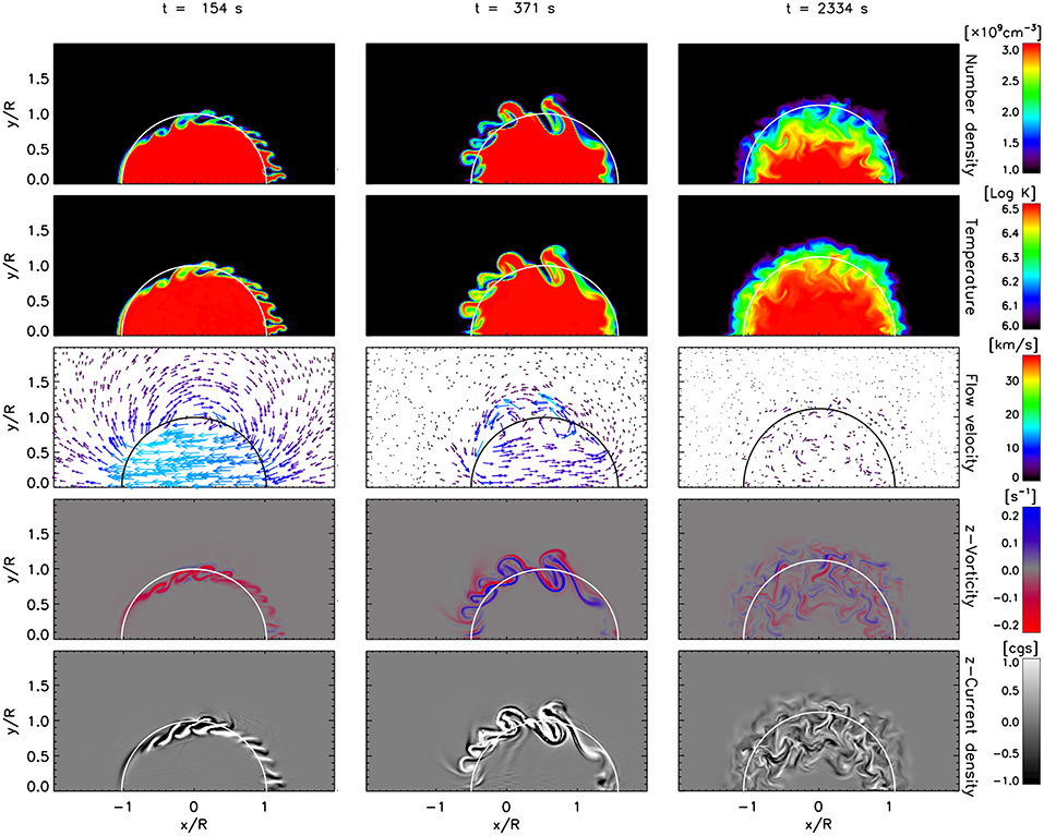
Figure 1. TWIKH vortices throughout, for a loop without initial boundary layer and no viscosity. From top to bottom rows we have the cross-section at the apex of the loop of, respectively, the total number density (in units of 10⁹ cm⁻³), the temperature (log T), the flow velocity (in km s⁻¹), the z−vorticity component (in s⁻¹) and the z−current density component (in cgs units). The 3 columns, from left to right, show 3 instances in time, respectively at t = 154 s ≈ P/2, t = 371 s ≈ 1.2 P, and t = 2, 334 s ≈ 7.4 P, where P = 315 s is the period of the kink mode. The half ellipse in white (or black in the flow velocity panels) corresponds to the ellipses calculated in section 3.2. See also the accompanying movie in the Supplementary Material.

FIGURE 2

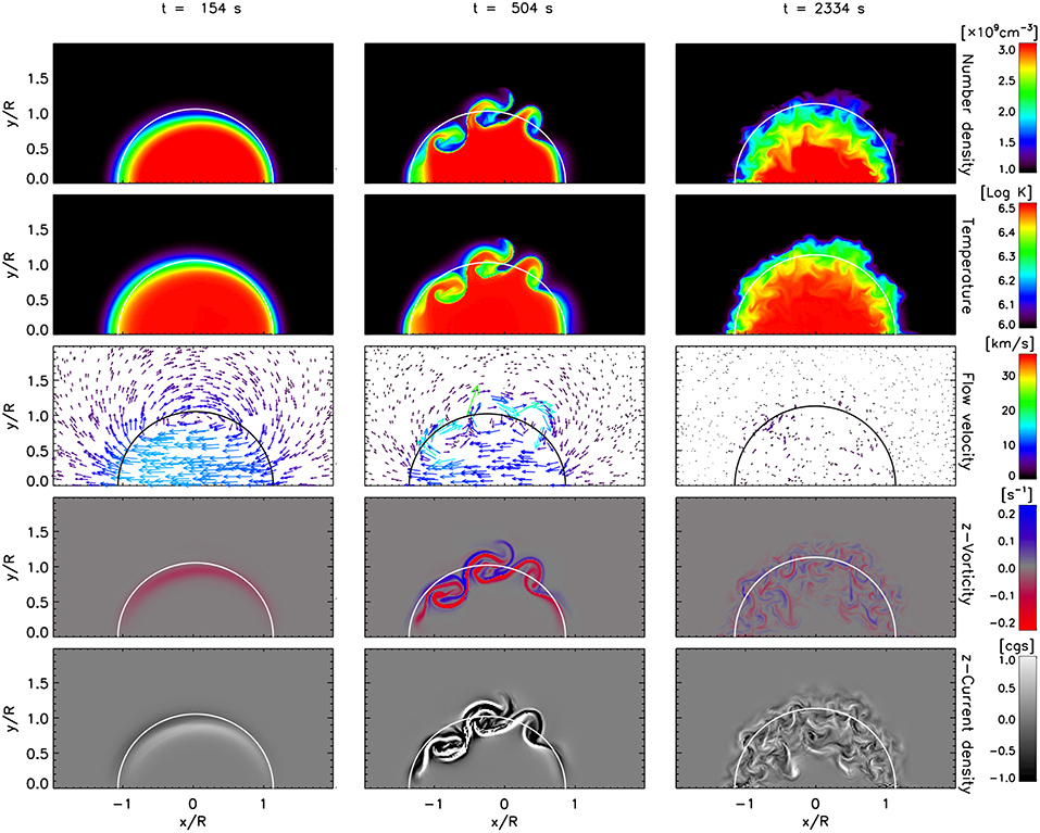
Figure 2. TWIKH vortices throughout for a loop with initial boundary layer and no viscosity. The same variables as in Figure 1 are shown, setting the same minima and maxima for better visualization. The same times are shown, except for the middle panel, for which we select a later time of t = 504 s ≈ 1.6 P, corresponding to the first formation of KHI vortices. See also the accompanying movie in the Supplementary Material.

FIGURE 3

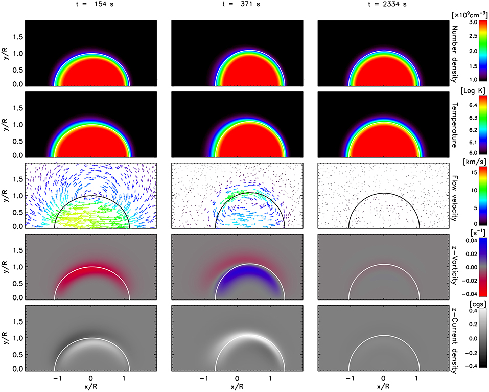
Figure 3. No TWIKH vortices for a loop with initial boundary layer and with enhanced viscosity. The same variables as in Figure 1 are shown. Note that the minima and maxima (notably for the velocities, vorticity and the current density) are smaller than for Figures 1, 2 due to the enhanced viscosity. The same times as in Figure 1 are shown. See also the accompanying movie in the Supplementary Material.

Due to the sharp contact discontinuity around the loop for the case without boundary layer and no viscosity, as soon as the perturbation starts, TWIKH rolls form around the side edges. This is expected since a flux tube (straight or twisted) is always unstable to the KHI [52], the sharp contact discontinuity and no viscosity ensures that the scale length where the velocity shear first exists is small enough to trigger these high azimuthal modes, and high azimuthal mode numbers have the highest growth rate. Additionally to these vortices at the side of the loop, we can see vortices at the wake. These vortices correspond to Rayleigh-Taylor (RT) vortices (and also lead to rolls in 3D, extending all along the loop), characterized by the finger-like structures (also produced for strong perturbations in dense, spicule-like structures with thicker boundary layers, [42]). As seen in Figure 2, these initial small-scale vortices (both, RT and KHI types) are absent for the case with initial boundary layer and no viscosity, since the scale length where the velocity shear first exists is larger than the size of these unstable modes.

After a period of oscillation (second column in Figures 1, 2) we note the appearance of larger vortices for the cases without viscosity. The boundary layer thickness is increased due to the vortices. After several periods (third column in Figures 1, 2) the global mode oscillation has largely damped (true for all cases), the boundary layer thickness has significantly increased to a radius or so without any significant difference between the models without viscosity and the vortices have expanded radially outwards and inwards. At a late stage only small-scale vortices remain, seen mainly in the vorticity and current density maps. On the other hand, the case with viscosity shows no dynamic instabilities and its boundary layer thickness remains largely unchanged between the initial and final stages (Figure 3).

In Figure 4 we show the evolution of the displacement of the loop axis at the apex and along the direction of oscillation. Since the models have slightly different maximum velocities and, correspondingly, different maximum displacements (all within 0.5 R and 0.6 R), to better visualize the damping we normalize the displacement by the respective maximum values. The displacement of the flux tube can be calculated in multiple ways. One way is to calculate the center of mass of the middle slice y = 0 at the apex for each time step. Another way is to fit a Gaussian of the density profile along the direction of oscillation at each time step. We choose the former method to calculate the damping, since this method suffers less influence from the vortices at the boundaries. In the rest of the paper, and in particular for section 3.2 we are more interested in the displacement of the boundary of the flux tube rather than the displacement of the loop's core, and hence we choose the second method for those cases.

FIGURE 4

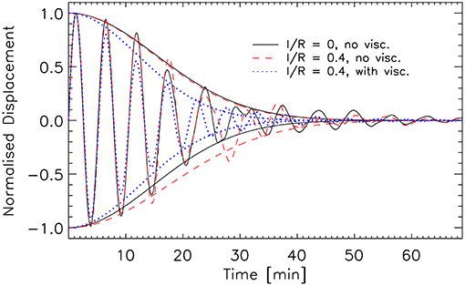
Figure 4. Displacement of the loop axis (at apex) with time. For each time step we define the center of the loop as the center of mass. The result over time is plotted for the loop with no initial boundary and no viscosity (black solid curve), with initial boundary layer and no viscosity (red dashed curve) and with initial boundary layer and viscosity (blue dotted curve). We also overlay the fits to the maxima and minima of each profile performed with a damped Gaussian function (see text for details).

In Figure 4 we can see that the effect on the damping time of not having an initial boundary layer and no viscosity is to extend it. This is expected since resonant absorption is delayed due to the initial absence of the boundary layer, which is created soon after by the KHI and RT vortices. As demonstrated by Pascoe et al. [68], Pascoe et al. [69], and Hood et al. [70], the damping of a fundamental kink mode due to resonant absorption is first governed by a Gaussian envelope and later on by an exponential envelope, and the switching time depends on the boundary layer thickness and the density contrast. To better quantify the damping time we therefore choose to fit the maxima of each profile with damped Gaussians of the form $v(t)exp(-t^2/L_g^2)$ (and we therefore define the damping time only by the Gaussian envelope time). Doing so we obtain damping times of 1,303 s (= 4.13 P), 1,280 s (= 4.06 P), and 1,030 s (= 3.27 P), respectively, for the cases of no initial boundary layer and no viscosity, initial boundary layer and no viscosity, and initial boundary layer and viscosity. The absence of an initial boundary layer means that the switch occurs slightly later and therefore less damping is obtained, as can indeed be seen. Also, by comparing the cases with and without viscosity, we can see that the presence of viscosity strongly reduces the damping time. In addition, at long times the cases with dynamic instabilities and no viscosity never damp completely. We discuss probable causes for this effect in section 4.

To compare with observations we can fit the envelopes of the oscillating profiles with an exponential rather than a Gaussian, and we find values between 2.2 and 2.6 P for all models. Accordingly, there is not much difference between the models since a boundary transition layer is rapidly formed due to the KHI. Comparing with linear damping (≈ 3.2 P, [21, 71]) we can see that the damping from our models with KHI with nonlinear amplitudes lead to stronger damping compared to the linear case, as has been found already by Magyar and Van Doorsselaere [40], who suggested this mechanism to explain the observed dependence of kink oscillation damping on the amplitude [72].

To see the extent of the KHI vortices we plot in Figure 5 the time-distance maps of density and z-vorticity cuts parallel to the y axis, moving with the flux tube and always crossing its center (where the center is defined with the Gaussian fit method as explained above). This method is better than tracking the center of mass since it takes more properly into account the radial extent of the KHI and RT vortices (relative to the Gaussian fit, the center of mass is displaced much less). Figure 5, and particularly the z-vorticity maps for the cases without viscosity show that the radial layers where the TWIKH rolls are generated move more rapidly inward than outward at a fast rate in the 1 − 2 periods (to t = 7 − 10 min), from y = 0.6 R to y = 1.3 R. Note that during this time interval the boundary layer thickness for the case without initial boundary layer increases steadily, while the increase is more abrupt for the case with initial boundary layer. This is due to the absence of small-scale KHI vortices initially for the latter model. The vortices then largely stop extending outward while they keep extending inward more gradually and at a steady rate until the end of the simulation (t = 69 min, corresponding to 13 periods), when the vortices have extended from y = 0.2 R to y = 1.4 R. The inward extension of vortices for the case with initial boundary layer seems to be slightly slower. On the other hand, the model with viscosity has a much lower vorticity that is concentrated around the resonant layer, and is diffused away relatively rapidly. An important consequence of this result is that impulsively excited kink waves generate turbulent loops, and thus that probably all loops in the solar corona are in a turbulent state.

FIGURE 5

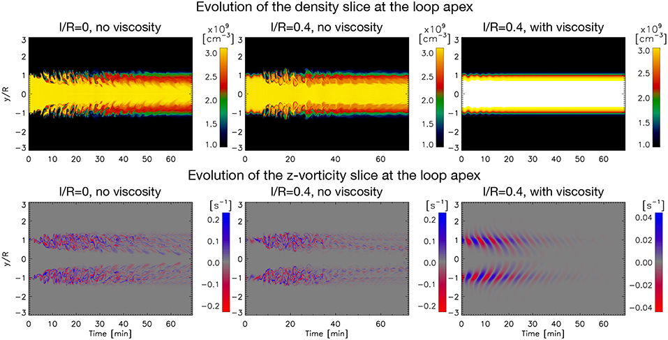
Figure 5. Outward and inward expansion of the vortices. For each loop model we take a parallel cut to the y axis across the loop passing through its center at each time step (see text for details on the procedure) and plot the resulting time-distance maps of the density (top panels) and z−vorticity (bottom panels) cuts. From left to right the columns correspond, respectively, to the model with no initial boundary layer and no viscosity, the model with initial boundary layer and no viscosity, and the model with initial boundary layer and viscosity. Note that the time range in the simulation with initial boundary layer and viscosity is slightly more extended in order to better visualize the inner vortices reaching the core of the loop. Note also that the extrema for the z−vorticity are much smaller for the enhanced viscosity case.

The density panels of Figure 5 for the cases without viscosity show that the first set of vortices at the boundary edge increase in size, producing deep entrances of the external material toward the loop center. The following sets of vortices that continuously develop are only internal and small-scale vortices, seen mainly in the vorticity maps since they do not produce large density changes. We can see that the changes in both the density and vorticity are slightly larger in the case of no initial boundary layer. The herringbone pattern seen in the vorticity panel reflects an apparent super slow wave propagation of the kind discussed by Kaneko et al. [73], produced by the phase mixing of the continuously produced KHI vortices.

3.2. Effect From Resonant Absorption

As investigated in, e.g., [43], the KHI smoothens the boundary layer. Hence, the influence of the KHI on resonant absorption is to increase the layer where the resonance (and phase mixing) occurs. In our simulation with no initial boundary layer we have only the KHI at first and only at later times (even if shortly after) the combined effect from KHI and resonant absorption. On the other hand, the simulation with enhanced viscosity has no KHI and only resonant absorption. Hence, by comparing these 3 models we can investigate the effect of the resonance on the KHI.

To investigate more carefully the development of resonant absorption we calculate the azimuthal velocity v_ϕ for each loop model, taking the center of the loop obtained through Gaussian fitting of the density profile explained previously. For each radial distance from the loop's center, we then calculate the azimuthal velocity amplitude by averaging the absolute value over ellipses around the center. We choose ellipses instead of circles since the loop cross-section deforms considerably due to high order radial modes and the KH and RT vortices [43, 55]. Since the ellipses are modified over time, we define the radial distance as the distance from the loop's center along the cut parallel to the y axis. For each time step, we find the semi-major and semi-minor axes of an ellipse along x and the axis parallel to y passing through the loop's center by locating (through interpolation) the position where the density is equal to 2n_e(t = 0), that is, the intermediate value between the internal and external density values at the beginning of the simulation. Therefore, we define this density point as the middle of the loop boundary layer. We also apply a temporal smoothing to the obtained variation of the ellipse axes over time, in order to get rid of the high frequency perturbations from the vortices. The temporal smoothening for the ellipse' s semi-axis parallel to the y axis has a very long boxcar width of 950 s in order to catch the long term variations only and not those from the high-frequency ones from the vortices. For a given time step we then take different self-similar ellipses with respect to the ellipse that fits the loop edge by changing the radial distance and keeping the same ratio between the axes. In Figures 1–3 (and the accompanying movies in the Supplementary Material) we overlay for each panel the ellipse fitting the loop edge obtained with this technique.

In Figure 6 we show for each loop model the time-distance diagram of the azimuthal velocity amplitude averaged along each self-similar ellipse located at different radial distances from the loop's center. The fringe pattern indicating high azimuthal velocity power has double the frequency of the kink mode, as expected. Note that the fringes within a short radius distance decrease in amplitude. This damping also reflects the damping seen in Figure 4. At the same time the amplitude of the region located within the contour where the kink speed is roughly equal to the local Alfvén speed increases. This is characteristic of resonant absorption. Note that for the model without initial boundary layer the amplitude within this contour reaches a maximum at t ≈ 15 min (roughly 3 periods) and extends to ≈ 26 min. For the model with initial boundary layer and no viscosity the maximum amplitude in the resonant layer is found at ≈ 7 min and extends to ≈ 23 min. On the other hand, the model with enhanced viscosity shows a maximum amplitude in the resonant layer at ≈ 7 min and extends to only ≈ 16 min due to the enhanced viscosity. Note that for the models with KHI the region of resonance is shifted inward toward the loop's center in time. We have checked that the kink speed is roughly constant throughout the simulation. Hence, this shift is due to the variation of the boundary layer due to the KHI. The regions outside of the contour show also significant amplitudes that grow with a similar rate as resonant absorption. At t > 30 min in both models most of the power within the resonant region has disappeared, while the regions of highest power have now shifted inwards (with a smaller power region outward). This shows that the energy from the resonant flows have transferred to the TWIKH rolls within the loop, themselves being triggered by the velocity shear produced by the resonance.

FIGURE 6

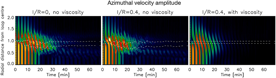
Figure 6. Azimuthal velocity amplitude from the loop's center. For each loop model, the azimuthal velocity amplitude (in absolute value) is calculated along moving ellipses around the loop's center that evolve through time. The ellipses are self-similar and their semi-major to semi-minor axis ratio matches the ellipse fitting the edge of the loop at each time step. Hence, for each ellipse at a given radial distance from the loop's center, we obtain an average value of the azimuthal velocity amplitude (in absolute value). The upper and lower dashed contours correspond, respectively, to the regions where the local Alfvén speed is 10% higher and 10% lower than the kink speed (see text for further details). From left to right the columns correspond, respectively, to the model with no initial boundary layer and no viscosity, the model with initial boundary layer and no viscosity, and the model with initial boundary layer and viscosity. Note that the color table has not been normalized to the same maximum between all loop models.

Hence we can see that the effect of the resonance on the KHI is to trigger the instability within the loop. The resonance acts as a localized energy reservoir by incrementing the azimuthal velocity shear in the loop's boundary layer.

3.3. High Azimuthal Wave Modes

We investigate now more closely the contribution from high azimuthal wavenumbers on the KHI dynamics. For this we follow the procedure of Terradas et al. [55] and calculate the Discrete Fourier Transform on the radial (v_rR) and azimuthal velocities (v_ϕR), and also on the density (ρ_R) at a distance R from the loop center. These quantities are computed over the ellipses described in the previous section. The mapping of these quantities along the circumference of the ellipses is uniform with respect to the angle ϕ. Using the same notation as in Terradas et al. [55] we calculate:

$\begin{array}{ll}G(p)=\frac{1}{N}{\displaystyle \sum _{k=0}^{N-1}}g(k)e^{-i\frac{2\pi }{N}pk},& (9)\end{array}$

where g(k) denotes either v_ϕR, v_rR or ρ_R, N is the total number of modes (p = 0, 1, …N − 1). We show for all models the contribution for the first 5 azimuthal modes to each quantity in Figure 7. It is worth to mention that due to the parity of v_ϕR, v_rR and ρ_R they are, respectively, purely imaginary, real and real functions, and that the dominant terms are shown in Figure 7 and the following figures.

FIGURE 7

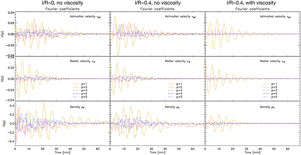
Figure 7. Fourier coefficients for the azimuthal and radial velocities and the density. We show the contribution of the azimuthal modes to each quantity along an ellipse fitting the edge of the loop by calculating the Discrete Fourier Transform (Equation 9). We only show the first 5 modes (see legend for line style).

The p = 1 mode has the dominant contribution overall for all models and for all quantities, except for ρ_R(t < 10 min). For the models developing KHI, the p = 2 mode has a significant power, similar or even higher to the p = 1 mode in some instances for the azimuthal velocity (and for the density at the beginning of the simulation). The higher order modes (p > 2) also have significant power. For the model without initial boundary layer, these higher order modes have the dominant power at the beginning of the simulation for the azimuthal velocity and density, compared to the model with initial boundary layer and no viscosity. For the latter, the higher order modes become dominant after 1 − 2 periods. And at the end of the simulations with KHI all modes for the azimuthal velocity have similar power.

As explained in Terradas et al. [55] in the absence of KHI the excitation of the p = 2 is produced mostly by the nonlinear effect of the inertia from the loop's motion (a squashing effect, described analytically in Ruderman and Goossens [56]), its frequency is double that of the kink mode, and the amplitude of the p = 2 mode is smaller than that of the p = 1 mode by the square of the amplitude. These properties can be seen in Figure 7 for the model with initial boundary layer and viscosity. The higher azimuthal wavenumbers increase their power only once the KHI has set in, as can be seen when comparing the 3 models. The higher order modes correspond to the small KHI and RT vortices that populate the edge of the loop, which are the fastest growing unstable modes in the model without initial boundary layer. In the case with an initial boundary layer the length scale over which velocity shear exists is larger, and therefore the first unstable modes have larger wavelength, and it is only in the nonlinear stage of the instability that higher order modes develop.

In the cases with KHI, all the high order modes have much higher power than that predicted by linear theory. The ellipses we construct are co-moving with the loop's edge and therefore we largely reduce the power coming from the deformation of the loop due to its inertia and also the nonlinear influence from the radial modes (hence, the power of p = 1 and p = 2). The large power still present in these modes and the higher order ones is due to the fact that the edge of the flux tube does not correspond to the spatial extent of the KHI vortices (as can be seen in Figures 1, 2 and the accompanying movies in the Supplementary Material). Hence, the vortices cross the ellipse boundary each time they form. This is particularly the case at the beginning of the simulation (when the deformation of the flux tube is large). Hence, the significant power at the beginning of the simulation without initial boundary layer comes mostly from the KHI. The observed increase of the power of all modes over the first 15 min (matching the time at maximum azimuthal velocity amplitude) is due to an influence from resonant absorption. The overall effect over the first 15 min is to have an apparent inverse energy cascade, where the lower order modes have increasing power in time (a trend that is particularly clear in the v_ϕR and ρ_R panels in Figure 7). Indeed, this is not observed in the case with initial boundary layer and no viscosity, for which once the higher order modes set in, all modes show an amplitude that remains roughly constant until t ≈ 20 min.

To investigate the generation of high azimuthal wavenumbers across each loop's cross section we now calculate the Discrete Fourier Transform on the azimuthal velocity along various of the self-similar ellipses located at different radii from the loop's center, described in the previous section. We thus take v_ϕr for r = 0.3 R, 0.4 R, 0.5 R, 0.6 R, 0.8 R, 1 R, 1.2 R and 1.4 R and show in Figures 8–10 (respectively for the loop without initial boundary layer and no viscosity, with initial boundary layer and no viscosity and with initial boundary layer and with viscosity) the corresponding contribution of the first 5 modes to the total signal.

FIGURE 8

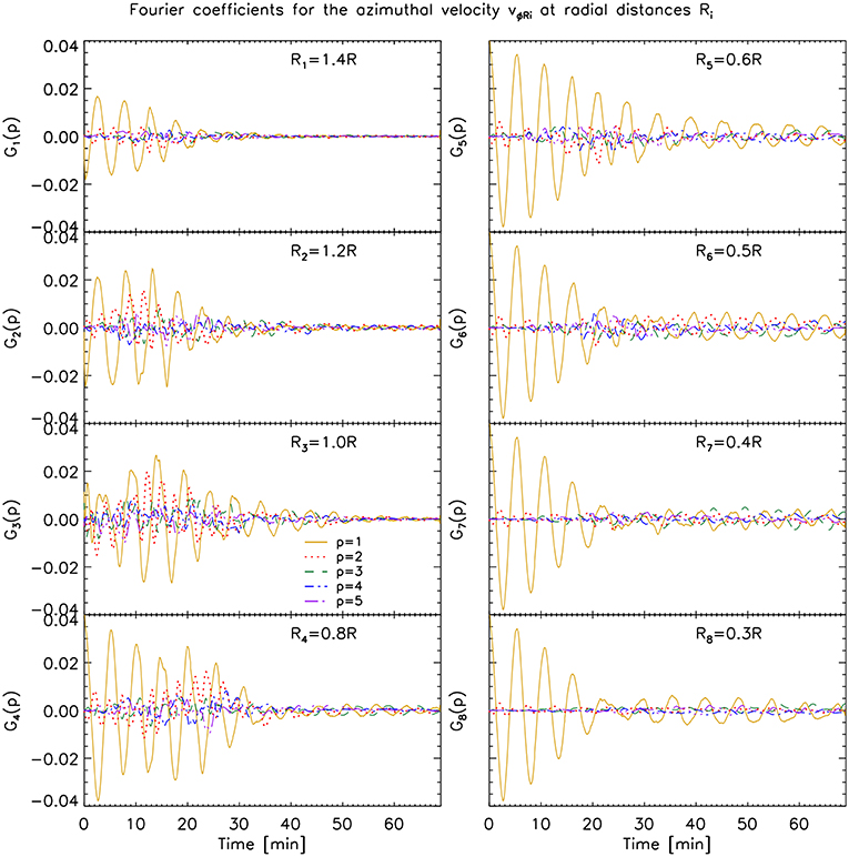
Figure 8. Fourier coefficients for the azimuthal velocity v_ϕRi at radial distances R_i for the case without initial boundary layer and no viscosity. We show the contribution of the azimuthal modes to the azimuthal velocity along self-similar ellipses whose semi-minor axis has various lengths R_i (as indicated in the panels). The semi-major to semi-minor axis ratio of all ellipses matches the ellipse fitting the edge of the loop at each time step (see text for further details). We show the first 5 azimuthal wave modes (see the legend for the corresponding line style).

FIGURE 9

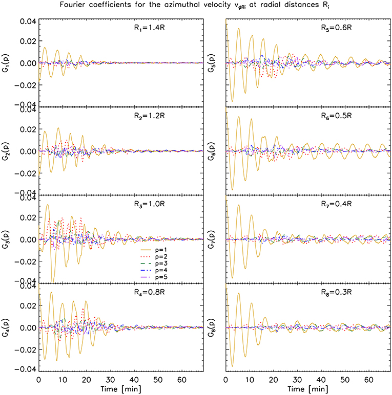
Figure 9. Fourier coefficients for the azimuthal velocity v_ϕRi at radial distances R_i for the case with initial boundary layer and no viscosity. See Figure 8 for more details.

FIGURE 10

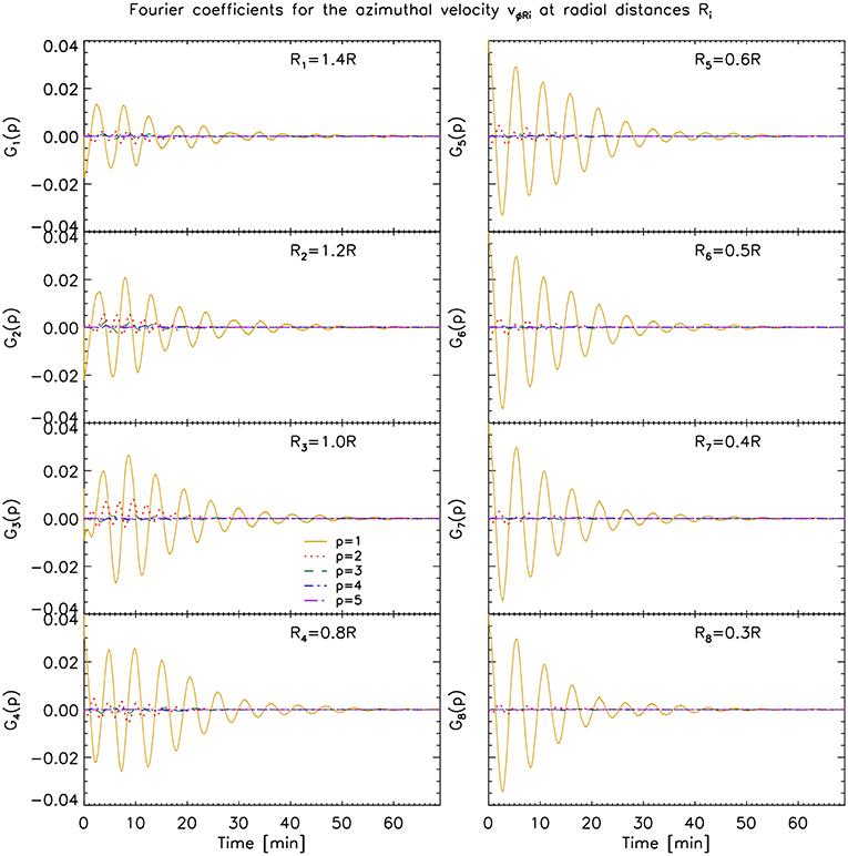
Figure 10. Fourier coefficients for the azimuthal velocity v_ϕRi at radial distances R_i for the case with initial boundary layer and with viscosity. See Figure 8 for more details.

Away from the region where most of the KHI occurs we mostly have the dipole (azimuthal) field generated by the kink mode (R₁ = 1.4 R panel in Figure 8), and its damping is similar to the damping observed in the same layer in the model without KHI. Note however, that higher order modes have nonetheless higher power even at this distance from the loop's center, reflecting a rapid but small influence of the KHI even at this distance. As we approach the KHI region in the models without viscosity, an increase of power in all modes can be seen, as noted previously (R₂ = 1.2 R, R₃ = 1 R, R₄ = 0.8 R panels in Figures 8, 9). As we pass from r = R to r = 0.8 R we can see for the model without initial boundary layer that the time of maximum power of all modes has been shifted to later times, from t = 15 min to t = 20 − 25 min. For the model with initial boundary layer, significant power in the high order modes at r = 0.8 R can be observed until t ≈ 20 min. This time shift (and time interval) matches the time of maximum resonance (or significant resonance), which is seen in Figure 6, and the spatial shift of the resonance from R to 0.8 R in the same time interval. Therefore, this further supports that the resonance is acting as catalyst of the KHI in both models without viscosity, irrespective of the presence of an initial boundary layer.

As we move further radially inward in the case without KHI, no significant difference in power for v_ϕRi is observed. On the other hand, for the cases with KHI we note a temporal shift to later times of the power increase in the high azimuthal wave modes. This suggests that the KHI self-induces itself, layer after layer deeper into the loop, starting from the resonant layer at the edge of the flux tube, which acts as an energy reservoir for the velocity shear. Moreover, even after the energy from the resonance has largely disappeared the inner vortices continue to trigger deeper KHI vortices. Thus, we can predict that both entire loops become eventually turbulent.

As mentioned in section 3 the model without initial boundary layer shows a slightly faster inward propagation of the KHI vortices. This can be explained by the fact that by allowing the boundary layer to develop naturally due to the KHI, the velocity shear that is produced by resonant absorption is slightly higher than in the model with initial boundary layer, thereby increasing the effectiveness for KHI.

4. Discussion and Conclusions

In this paper we have taken three different loop models: a coronal loop without an initial boundary layer, a coronal loop with initial boundary layer, and a coronal loop with initial boundary layer and unrealistically high viscosity. We have simulated a perturbation leading to a fundamental kink mode, matching the usually observed amplitudes of transverse MHD waves. Although the case without an initial boundary layer is a rather extreme case of coronal loop formation and may be unrealistic, we do this mainly to investigate the effect that resonant absorption has on the development of the KHI. Also, a possible physical justification for sharp boundary layers is the case of a highly spatially confined energy deposition, for instance through magnetic reconnection, that would result in a spatially confined chromospheric evaporation and therefore sharp boundary layer for a loop.

By taking a sharp boundary layer we manage to delay the onset of resonant absorption in that loop compared to the case with initial boundary layer. As soon as the loop starts oscillating the small length scale over which the velocity shear takes place at the edges of the flux tube triggers the TWIKH rolls. At the wake of the flux tube RT rolls are also generated. High azimuthal wave modes are generated first, as expected since they are the fastest growing modes [52]. Lower and more energetic wave modes grow after 1 − 2 periods, not only from the KHI but also due to the squashing of the loop produced by the inertia [55, 56]. These low order modes are the first ones that grow in the case of an initial boundary layer. Higher order modes follow as well in the nonlinear stage of the KHI. Hence, this initial process can be seen as an apparent inverse energy cascade, produced mainly by the initially sharp boundary layer in that loop model. Due to KHI, the layer thickens quickly, and with it resonant absorption starts to take place. As the resonance reaches a maximum amplitude so does the power of high azimuthal wave modes. The time interval and spatial extent of significant resonance power matches the time interval and spatial extent of significant power in the high order azimuthal modes. The resonance triggers, in particular, TWIKH rolls radially inwards inside the loops and a self-inducing process of TWIKH rolls occurs gradually deeper at a steady rate (producing a super slow apparent wave propagation of the kind discussed by Kaneko et al. [73]) until they end up covering basically the entire loops.

In this paper, we have proven that also impulsively excited loops, regardless of their initial boundary layer thickness eventually render the loop's cross-section to a turbulent state, as was previously proven for continuously driven loops [46]. This has as important implication that probably all observed loops (which undergo transverse oscillations at some point in their life, [20]) are in a turbulent state.

This investigation shows that resonant absorption is key to energize TWIKH rolls and spread them all over the loop. In our cases of only one perturbation only high azimuthal wave modes reach the loop center, and therefore the energy transfer to the inner layers is small in the absence of continuous driving. K-H rolls have also been analytically and numerically predicted from the shear flow of other transverse waves, such as torsional Alfvén waves [37, 47, 51, 74]. Our results suggest that in the absence of continuous driving the absence of resonant absorption in these cases may lead to important differences. Namely, the absence of velocity shear at the resonance layer would fail to induce inner KHI vortices eventually making the entire loop turbulent in the self-induction process we have found.

In the case of the loop with an initially present boundary layer, resonant absorption starts occurring immediately after the impulsive excitation, which produces a slightly stronger damping than in a case with no initial boundary layer and hence a relatively faster switch from a Gaussian damping profile to an exponential damping profile [68–70]. From Figure 4 we can see that some differences indeed arise between cases with or without initial boundary layer. But more importantly, there are strong deviations from both the Gaussian and exponential damping during the evolution, due to the KHI. Since the switch between the Gaussian and exponential damping profiles is mostly defined by the density ratio and the boundary layer thickness, It is usually considered that the envelope can be used for seismology. This is of course not valid in our models, since this switch is controlled by the width of the boundary layer that varies extremely over time due to KHI.

Based on the comparison between the models with and without boundary layers leading to TWIKH rolls, we predict that loops with larger boundary transitions would lead to somewhat longer times (but on the same order) for the loops to become fully turbulent. This is because thicker boundary layers imply lower velocity shear and hence a delay on the onset of the KHI. On the other hand, a loop with a thicker boundary transition implies a more energetic resonant flow, and therefore a larger energy reservoir for the self-inducing process of KHI inwards. Hence, the vortices reaching the loop core may be larger (more energetic).

Another interesting feature seen in Figure 4 and in Figures 8–10 is that the global kink mode (p = 1) does not seem to damp completely for t > 30 min within the flux tube (for r < 0.5 R). This result was also noticed by Magyar and Van Doorsselaere [40], and they suggested an explanation based on KHI energy being transferred to the core of the loop. Indeed, our experiments confirm this hypothesis. It is also possible to have a feedback mechanism from the TWIKH rolls on the loop, due to an overall vorticity imbalance (and therefore momentum imbalance) within the loop due to the TWIKH rolls, as is observed in the phenomenon of vortex shedding [75, 76]. The slight change in period and beat at t ≈ 25 − 30 min for the inner shells and for the center of mass oscillation (Figure 4), compared to the model without KHI, supports this theory. If true, this could be another possible mechanism to generate the observed decayless transverse oscillations [20, 77, 78].

Given that loops eventually become fully turbulent following a kink oscillation, a relevant question is the timescale on which this happens. This is particularly relevant in the context of coronal heating, since the small scales produced by dynamic instabilities can be a means for wave dissipation. Our models show that the loops become fully turbulent after 13 − 14 periods (69 − 72 min), which is a very long timescale for coronal heating and therefore the wave dissipation rate over the entire loop may be too small to account for coronal heating. In the cases of continuous driving at the natural frequency of the loop, as in the numerical experiments by Karampelas and Van Doorsselaere [46], the situation improves, since the amplitudes obtained at the apex are on average stronger and the loops become fully turbulent after ≈ 7.5 periods (2000 s in their model), which may still be considered long for coronal heating.

Data Availability

The datasets generated for this study are available on request to the corresponding author.

Author Contributions

PA conducted the simulations and analysis, TVD has provided feedback on the analysis of the results.

Funding

PA acknowledges funding from his STFC Ernest Rutherford Fellowship (No. ST/R004285/1). TVD was funded by GOA-2015-014 (KU Leuven). This project has received funding from the European Research Council (ERC) under the European Union's Horizon 2020 research and innovation programme (grant agreement No. 724326).

Conflict of Interest Statement

The authors declare that the research was conducted in the absence of any commercial or financial relationships that could be construed as a potential conflict of interest.

The reviewer MR declared a past co-authorship with one of the authors (TVD) to the handling editor.

Acknowledgments

Numerical computations were carried out on Cray XC50 at the Center for Computational Astrophysics, NAOJ.

Supplementary Material

The Supplementary Material for this article can be found online at: https://www.frontiersin.org/articles/10.3389/fphy.2019.00085/full#supplementary-material

Video 1. TWIKH vortices throughout, for a loop without initial boundary layer and no viscosity. From top to bottom rows we have the cross-section at the apex of the loop of, respectively, the total number density (in units of 10⁹ cm⁻³), the temperature (log T), the flow velocity (in km s⁻¹), the z−vorticity component (in s⁻¹) and the z−current density component (in cgs units). The half ellipse in white (or black in the flow velocity panels) corresponds to the ellipses calculated in section 3.2. This animation corresponds to Figure 1.

Video 2. TWIKH vortices throughout for a loop with initial boundary layer and no viscosity. The same variables as in Video 1 (or Figure 1) are shown, setting the same minima and maxima for better visualisation. This animation corresponds to Figure 2.

Video 3. No TWIKH vortices for a loop with initial boundary layer and with enhanced viscosity. The same variables as in Video 1 (or Figure 1) are shown. Note that the minima and maxima (notably for the velocities, vorticity, and the current density) are smaller than for Videos 1, 2 (Figures 1, 2) due to the enhanced viscosity. This animation corresponds to Figure 3.

References

1. Viall NM, Klimchuk JA. Evidence for widespread cooling in an active region observed with the SDO atmospheric imaging assembly. Astrophys J. (2012) 753:35. doi: 10.1088/0004-637X/753/1/35

CrossRef Full Text | Google Scholar

2. Viall NM, Klimchuk JA. Modeling the line-of-sight integrated emission in the corona: implications for coronal heating. Astrophys J. (2013) 771:115. doi: 10.1088/0004-637X/771/2/115

CrossRef Full Text | Google Scholar

3. Magyar N, Van Doorsselaere T. The instability and non-existence of multi-stranded loops when driven by transverse waves. Astrophys J. (2016) 823:82. doi: 10.3847/0004-637X/823/2/82

CrossRef Full Text | Google Scholar

4. Brooks DH, Warren HP, Ugarte-Urra I, Winebarger AR. High spatial resolution observations of loops in the solar corona. Astrophys J Lett. (2013) 772:L19. doi: 10.1088/2041-8205/772/2/L19

CrossRef Full Text | Google Scholar

5. Brooks DH, Reep JW, Warren HP. Properties and modeling of unresolved fine structure loops observed in the solar transition region by IRIS. Astrophys J Lett. (2016) 826:L18. doi: 10.3847/2041-8205/826/2/L18

CrossRef Full Text | Google Scholar

6. Solanki SK. Smallscale solar magnetic fields-an overview. Space Sci Rev. (1993) 63:1–2. doi: 10.1007/BF00749277

CrossRef Full Text | Google Scholar

7. Reale F. Coronal loops: observations and modeling of confined plasma. Living Rev Solar Phys. (2010) 7:5. doi: 10.12942/lrsp-2010-5

CrossRef Full Text | Google Scholar

8. Watko JA, Klimchuk JA. Width Variations along Coronal Loops Observed by TRACE. solar Phys. (2000) 193:77–92. doi: 10.1007/978-94-010-0860-0_5

CrossRef Full Text | Google Scholar

9. Peter H, Bingert S, Klimchuk JA, de Forest C, Cirtain JW, Golub L, et al. Structure of solar coronal loops: from miniature to large-scale. Astron Astrophys. (2013) 556:A104. doi: 10.1051/0004-6361/201321826

CrossRef Full Text | Google Scholar

10. Antolin P, Rouppe van der Voort L. Observing the fine structure of loops through high-resolution spectroscopic observations of coronal rain with the CRISP instrument at the swedish solar telescope. Astrophys J. (2012) 745:152. doi: 10.1088/0004-637X/745/2/152

CrossRef Full Text | Google Scholar

11. Antolin P, Vissers G, Pereira TMD, Rouppe van der Voort L, Scullion E. The multithermal and multi-stranded nature of coronal rain. Astrophys J. (2015) 806:81. doi: 10.1088/0004-637X/806/1/81

CrossRef Full Text | Google Scholar

12. Cargill PJ, De Moortel I, Kiddie G. Coronal density structure and its role in wave damping in loops. Astrophys J. (2016) 823:31. doi: 10.3847/0004-637X/823/1/31

CrossRef Full Text | Google Scholar

13. Pascoe DJ, Goddard CR, Nisticò G, Anfinogentov S, Nakariakov VM. Coronal loop seismology using damping of standing kink oscillations by mode coupling. Astron Astrophys. (2016) 589:A136. doi: 10.1051/0004-6361/201628255

CrossRef Full Text | Google Scholar

14. Pascoe DJ, Anfinogentov S, Nisticò G, Goddard CR, Nakariakov VM. Coronal loop seismology using damping of standing kink oscillations by mode coupling. II. additional physical effects and Bayesian analysis. Astron Astrophys. (2017) 600:A78. doi: 10.1051/0004-6361/201629702

CrossRef Full Text | Google Scholar

15. Aschwanden MJ, Fletcher L, Schrijver CJ, Alexander D. Coronal loop oscillations observed with the transition region and coronal explorer. Astrophys J. (1999) 520:880–94. doi: 10.1086/307502

CrossRef Full Text | Google Scholar

16. Nakariakov VM, Ofman L, Deluca EE, Roberts B, Davila JM. TRACE observation of damped coronal loop oscillations: implications for coronal heating. Science. (1999) 285:862–4. doi: 10.1126/science.285.5429.862

PubMed Abstract | CrossRef Full Text | Google Scholar

17. De Moortel I, Nakariakov VM. Magnetohydrodynamic waves and coronal seismology: an overview of recent results. R Soc Lond Philos Trans A. (2012) 370:3193–216. doi: 10.1098/rsta.2011.0640

PubMed Abstract | CrossRef Full Text | Google Scholar

18. Tomczyk S, McIntosh SW, Keil SL, Judge PG, Schad T, Seeley DH, et al. Alfvén waves in the solar corona. Science. (2007) 317:1192. doi: 10.1126/science.1143304

PubMed Abstract | CrossRef Full Text | Google Scholar

19. Arregui I, Oliver R, Ballester JL. Prominence oscillations. Living Rev Solar Phys. (2012) 9:2. doi: 10.12942/lrsp-2012-2

CrossRef Full Text | Google Scholar

20. Anfinogentov SA, Nakariakov VM, Nisticò G. Decayless low-amplitude kink oscillations: a common phenomenon in the solar corona? Astron Astrophys. (2015) 583:A136. doi: 10.1051/0004-6361/201526195

CrossRef Full Text | Google Scholar

21. Goossens M, Andries J, Aschwanden MJ. Coronal loop oscillations. An interpretation in terms of resonant absorption of quasi-mode kink oscillations. Astron Astrophys. (2002) 394:L39–42. doi: 10.1051/0004-6361:20021378

CrossRef Full Text | Google Scholar

22. Goossens M, Andries J, Arregui I. Damping of magnetohydrodynamic waves by resonant absorption in the solar atmosphere. R Soc Lond Philos Trans A. (2006) 364:433–46. doi: 10.1098/rsta.2005.1708

PubMed Abstract | CrossRef Full Text | Google Scholar

23. Van Doorsselaere T, Andries J, Poedts S, Goossens M. Damping of coronal loop oscillations: calculation of resonantly damped kink oscillations of one-dimensional nonuniform loops. Astrophys J. (2004) 606:1223–32. doi: 10.1086/383191

CrossRef Full Text | Google Scholar

24. Goossens M, Erdélyi R, Ruderman MS. Resonant MHD Waves in the Solar Atmosphere. Space Sci Rev. (2011) 158:289–338. doi: 10.1007/s11214-010-9702-7

CrossRef Full Text | Google Scholar

25. Verwichte E, Van Doorsselaere T, White RS, Antolin P. Statistical seismology of transverse waves in the solar corona. Astron Astrophys. (2013) 552:A138. doi: 10.1051/0004-6361/201220456

CrossRef Full Text | Google Scholar

26. Goddard CR, Nisticò G, Nakariakov VM, Zimovets IV. A statistical study of decaying kink oscillations detected using SDO/AIA. Astron Astrophys. (2016) 585:A137. doi: 10.1051/0004-6361/201527341

CrossRef Full Text | Google Scholar

27. Allan W, Wright AN. Magnetotail waveguide: fast and Alfvén waves in the plasma sheet boundary layer and lobe. J. Geophys. Res. (2000) 105:317–28. doi: 10.1029/1999JA900425

CrossRef Full Text | Google Scholar

28. Pascoe DJ, Wright AN, De Moortel I. Coupled Alfvén and kink oscillations in coronal loops. Astrophys J. (2010) 711:990–6. doi: 10.1088/0004-637X/711/2/990

CrossRef Full Text | Google Scholar

29. De Moortel I, Pascoe DJ, Wright AN, Hood AW. Transverse, propagating velocity perturbations in solar coronal loops. Plasma Phys Control Fusion. (2016) 58:014001. doi: 10.1088/0741-3335/58/1/014001

CrossRef Full Text | Google Scholar

30. Terradas J, Goossens M, Verth G. Selective spatial damping of propagating kink waves due to resonant absorption. Astron Astrophys. (2010) 524:A23. doi: 10.1051/0004-6361/201014845

CrossRef Full Text | Google Scholar

31. Verth G, Terradas J, Goossens M. Observational evidence of resonantly damped propagating kink waves in the solar corona. Astrophys J Lett. (2010) 718:L102–5. doi: 10.1088/2041-8205/718/2/L102

CrossRef Full Text | Google Scholar

32. Terradas J, Arregui I, Oliver R, Ballester JL, Andries J, Goossens M. Resonant absorption in complicated plasma configurations: applications to multistranded coronal loop oscillations. Astrophys J. (2008) 679:1611–20. doi: 10.1086/586733

CrossRef Full Text | Google Scholar

33. Pascoe DJ, Wright AN, De Moortel I. Propagating coupled Alfvén and kink oscillations in an arbitrary inhomogeneous corona. Astrophys J. (2011) 731:73. doi: 10.1088/0004-637X/731/1/73

CrossRef Full Text | Google Scholar

34. Goossens M, Ruderman MS, Hollweg JV. Dissipative MHD solutions for resonant Alfven waves in 1-dimensional magnetic flux tubes. Solar Phys. (1995) 157:75–102. doi: 10.1007/BF00680610

CrossRef Full Text | Google Scholar

35. Goossens M, Soler R, Terradas J, Van Doorsselaere T, Verth G. The transverse and rotational motions of magnetohydrodynamic kink waves in the solar atmosphere. Astrophys J. (2014) 788:9. doi: 10.1088/0004-637X/788/1/9

CrossRef Full Text | Google Scholar

36. Antolin P, Yokoyama T, Van Doorsselaere T. Fine strand-like structure in the solar corona from magnetohydrodynamic transverse oscillations. Astrophys J Lett. (2014) 787:L22. doi: 10.1088/2041-8205/787/2/L22

CrossRef Full Text | Google Scholar

37. Browning PK, Priest ER. Kelvin-Helmholtz instability of a phased-mixed Alfven wave. Astron Astrophys. (1984) 131:283–90.

Google Scholar

38. Antolin P, Okamoto TJ, De Pontieu B, Uitenbroek H, Van Doorsselaere T, Yokoyama T. Resonant absorption of transverse oscillations and associated heating in a solar prominence. II. numerical aspects. Astrophys J. (2015) 809:72. doi: 10.1088/0004-637X/809/1/72

CrossRef Full Text | Google Scholar

39. Terradas J, Andries J, Goossens M, Arregui I, Oliver R, Ballester JL. Nonlinear instability of kink oscillations due to shear motions. Astrophys J Lett. (2008) 687:L115–8. doi: 10.1086/593203

CrossRef Full Text | Google Scholar

40. Magyar N, Van Doorsselaere T. Damping of nonlinear standing kink oscillations: a numerical study. Astron Astrophys. (2016) 595:A81. doi: 10.1051/0004-6361/201629010

CrossRef Full Text | Google Scholar

41. Karampelas K, Van Doorsselaere T, Antolin P. Heating by transverse waves in simulated coronal loops. Astron Astrophys. (2017) 604:A130. doi: 10.1051/0004-6361/201730598

CrossRef Full Text | Google Scholar

42. Antolin P, Schmit D, Pereira TMD, De Pontieu B, De Moortel I. Transverse wave induced kelvin-helmholtz rolls in spicules. Astrophys J. (2018) 856:44. doi: 10.3847/1538-4357/aab34f

CrossRef Full Text | Google Scholar

43. Antolin P, De Moortel I, Van Doorsselaere T, Yokoyama T. Observational signatures of transverse magnetohydrodynamic waves and associated dynamic instabilities in coronal flux tubes. Astrophys J. (2017) 836:219. doi: 10.3847/1538-4357/aa5eb2

CrossRef Full Text | Google Scholar

44. Okamoto TJ, Antolin P, De Pontieu B, Uitenbroek H, Van Doorsselaere T, Yokoyama T. Resonant absorption of transverse oscillations and associated heating in a solar prominence. I. observational aspects. Astrophys J. (2015) 809:71. doi: 10.1088/0004-637X/809/1/71

CrossRef Full Text | Google Scholar

45. Van Doorsselaere T, Antolin P, Karampelas K. Broadening of the differential emission measure by multi-shelled and turbulent loops. Astron Astrophys. (2018) 620:A65. doi: 10.1051/0004-6361/201834086

CrossRef Full Text | Google Scholar

46. Karampelas K, Van Doorsselaere T. Simulations of fully deformed oscillating flux tubes. Astron Astrophys. (2018) 610:L9. doi: 10.1051/0004-6361/201731646

CrossRef Full Text | Google Scholar

47. Guo M, Van Doorsselaere T, Karampelas K, Li B, Antolin P, De Moortel I. Heating effects from driven transverse and Alfvén waves in coronal loops. Astrophys J. (2019) 870:55. doi: 10.3847/1538-4357/aaf1d0

CrossRef Full Text | Google Scholar

48. Ofman L, Thompson BJ. SDO/AIA observation of kelvin-helmholtz instability in the solar corona. Astrophys J Lett. (2011) 734:L11. doi: 10.1088/2041-8205/734/1/L11

CrossRef Full Text | Google Scholar

49. Zhelyazkov I, Zaqarashvili TV, Chandra R, Srivastava AK, Mishonov T. Kelvin-Helmholtz instability in solar cool surges. Adv Space Res. (2015) 56:2727–37. doi: 10.1016/j.asr.2015.05.003

CrossRef Full Text | Google Scholar

50. Li X, Zhang J, Yang S, Hou Y, Erdélyi R. Observing kelvin–helmholtz instability in solar blowout jet. Sci Rep. (2018) 8:8136. doi: 10.1038/s41598-018-26581-4

PubMed Abstract | CrossRef Full Text | Google Scholar

51. Zaqarashvili TV, Zhelyazkov I, Ofman L. Stability of rotating magnetized jets in the solar atmosphere. I. kelvin-Helmholtz instability. Astrophys J. (2015) 813:123. doi: 10.1088/0004-637X/813/2/123

CrossRef Full Text | Google Scholar

52. Barbulescu M, Ruderman MS, Van Doorsselaere T, Erdélyi R. An analytical model of the Kelvin-Helmholtz instability of transverse coronal loop oscillations. Astrophys J. (2019) 870:108. doi: 10.3847/1538-4357/aaf506

CrossRef Full Text | Google Scholar

53. Hillier A, Barker A, Arregui I, Latter H. On Kelvin-Helmholtz and parametric instabilities driven by coronal waves. Month Notices R Astron Soc. (2019) 482:1143–53. doi: 10.1093/mnras/sty2742

CrossRef Full Text | Google Scholar

54. Howson TA, De Moortel I, Antolin P. Energetics of the Kelvin-Helmholtz instability induced by transverse waves in twisted coronal loops. Astron Astrophys. (2017) 607:A77. doi: 10.1051/0004-6361/201731178

CrossRef Full Text | Google Scholar

55. Terradas J, Magyar N, Van Doorsselaere T. Effect of magnetic twist on nonlinear transverse kink oscillations of line-tied magnetic flux Tubes. Astrophys J. (2018) 853:35. doi: 10.3847/1538-4357/aa9d0f

CrossRef Full Text | Google Scholar

56. Ruderman MS, Goossens M. Nonlinear kink oscillations of coronal magnetic loops. Solar Phys. (2014) 289:1999–2020. doi: 10.1007/s11207-013-0446-x

CrossRef Full Text | Google Scholar

57. Sato T, Hayashi T. Externally driven magnetic reconnection and a powerful magnetic energy converter. Phys Fluids. (1979) 22:1189–202. doi: 10.1063/1.862721

CrossRef Full Text | Google Scholar

58. Ugai M. Computer studies on development of the fast reconnection mechanism for different resistivity models. Phys Fluids B (1992) 4:2953–63. doi: 10.1063/1.860458

CrossRef Full Text | Google Scholar

59. Miyagoshi T, Yokoyama T. Magnetohydrodynamic simulation of solar coronal chromospheric evaporation jets caused by magnetic reconnection associated with magnetic flux emergence. Astrophys J. (2004) 614:1042–53. doi: 10.1086/423731

CrossRef Full Text | Google Scholar

60. Yokoyama T, Shibata K. What is the condition for fast magnetic reconnection? Astrophys J Lett. (1994) 436:L197–200. doi: 10.1086/187666

CrossRef Full Text | Google Scholar

61. Lapidus A. A detached shock calculation by second-order finite differences. J Comput Phys. (1967) 2:154–77. doi: 10.1016/0021-9991(67)90032-0

CrossRef Full Text | Google Scholar

62. Kudoh T, Matsumoto R, Shibata K. Numerical MHD simulation of astrophysical problems by using CIP-MOCCT method. Comput Fluid Dyn J. (1999) 8:56–68.

Google Scholar

63. Yabe T, Aoki T. A universal solver for hyperbolic equations by cubic-polynomial interpolation I. One-dimensional solver. Comput Phys Commun. (1991) 66:219–32. doi: 10.1016/0010-4655(91)90071-R

CrossRef Full Text | Google Scholar

64. Evans CR, Hawley JF. Simulation of magnetohydrodynamic flows - A constrained transport method. Astrophys J. (1988) 332:659–77. doi: 10.1086/166684

CrossRef Full Text | Google Scholar

65. Stone JM, Norman ML. ZEUS-2D: a radiation magnetohydrodynamics code for astrophysical flows in two space dimensions. I - The hydrodynamic algorithms and tests. Astrophys J Suppl. (1992) 80:753–90. doi: 10.1086/191680

CrossRef Full Text | Google Scholar

66. Yabe T, Xiao F. Description of complex and sharp interface during Shock wave interaction with liquid drop. J Phys Soc Jpn. (1993) 62:2537. doi: 10.1143/JPSJ.62.2537

CrossRef Full Text | Google Scholar

67. Kudoh T, Matsumoto R, Shibata K. Magnetically driven jets from accretion disks. III. 2.5-dimensional nonsteady simulations for thick disk case. Astrophys J. (1998) 508:186–99. doi: 10.1086/306377

CrossRef Full Text | Google Scholar

68. Pascoe DJ, Hood AW, de Moortel I, Wright AN. Spatial damping of propagating kink waves due to mode coupling. Astron Astrophys. (2012) 539:A37. doi: 10.1051/0004-6361/201117979

CrossRef Full Text | Google Scholar

69. Pascoe DJ, Hood AW, De Moortel I, Wright AN. Damping of kink waves by mode coupling. II. Parametric study and seismology. Astron Astrophys. (2013) 551:A40. doi: 10.1051/0004-6361/201220620

CrossRef Full Text | Google Scholar

70. Hood AW, Ruderman M, Pascoe DJ, De Moortel I, Terradas J, Wright AN. Damping of kink waves by mode coupling. I. Analytical treatment. Astron Astrophys. (2013) 551:A39. doi: 10.1051/0004-6361/201220617

CrossRef Full Text | Google Scholar

71. Ruderman MS, Roberts B. The damping of coronal loop oscillations. Astrophys J. (2002) 577:475–86. doi: 10.1086/342130

CrossRef Full Text | Google Scholar

72. Goddard CR, Nakariakov VM. Dependence of kink oscillation damping on the amplitude. Astron Astrophys. (2016) 590:L5. doi: 10.1051/0004-6361/201628718

CrossRef Full Text | Google Scholar

73. Kaneko T, Goossens M, Soler R, Terradas J, Van Doorsselaere T, Yokoyama T, et al. Apparent cross-field superslow propagation of magnetohydrodynamic waves in solar plasmas. Astrophys J. (2015) 812:121. doi: 10.1088/0004-637X/812/2/121

CrossRef Full Text | Google Scholar

74. Srivastava AK, Shetye J, Murawski K, Doyle JG, Stangalini M, Scullion E, et al. High-frequency torsional Alfvén waves as an energy source for coronal heating. Sci Rep. (2017) 7:43147. doi: 10.1038/srep43147

PubMed Abstract | CrossRef Full Text | Google Scholar

75. Gruszecki M, Nakariakov VM, van Doorsselaere T, Arber TD. Phenomenon of Alfvénic vortex shedding. Phys Rev Lett. (2010) 105:055004. doi: 10.1103/PhysRevLett.105.055004

PubMed Abstract | CrossRef Full Text | Google Scholar

76. Emonet T, Moreno-Insertis F, Rast MP. The zigzag path of buoyant magnetic tubes and the generation of vorticity along their periphery. Astrophys J. (2001) 549:1212–20. doi: 10.1086/319469

CrossRef Full Text | Google Scholar

77. Anfinogentov S, Nisticò G, Nakariakov VM. Decay-less kink oscillations in coronal loops. Astron Astrophys. (2013) 560:A107. doi: 10.1051/0004-6361/201322094

CrossRef Full Text | Google Scholar

78. Nisticò G, Nakariakov VM, Verwichte E. Decaying and decayless transverse oscillations of a coronal loop. Astron Astrophys. (2013) 552:A57. doi: 10.1051/0004-6361/201220676

CrossRef Full Text | Google Scholar