Cross-Frequency Interactions During Information Flow in Complex Brain Networks Are Facilitated by Scale-Free Properties

Introduction

The study of information flow and transport in complex biological and social networks by means of random walks has attracted increasing interest in recent years [1–4]. Random walks [5] are the processes by which randomly-moving objects wander away from their starting location. In the past decades, there has been considerable progress in characterizing first passage times, or the amount of time it takes a random walker to reach a target [6–9]. However, previous works have neglected the study of the temporal dynamics of the information flow in the network, which depends on how the walkers move and not just on their arrival time. Thus, we lack knowledge about how the different temporal scales in the information flow arise from the topological structure of the network, whether they interact, and how they do it. This paper aims to address such knowledge gap.

We hypothesize that random walk processes in complex networks have associated multiple temporal scales, depending on the network structure. Furthermore, these temporal scales may interact. To study these scales, and their interaction, we use the empirical mode decomposition (EMD) [10], an adaptive and data-driven method that decomposes non-linear and non-stationary signals, like the movement of the random walkers, into fundamental modes of oscillations called intrinsic mode functions (IMFs), without the need for a predefined model as is the case for Fourier and wavelet transforms. Since IMFs are associated with different oscillatory modes, their interactions correspond to the phenomenon known as cross-frequency coupling (CFC) [11]. Three types of CFC are most widely studied: phase-amplitude coupling (PAC), the phenomenon where the instantaneous phase of a low frequency oscillation modulates the instantaneous amplitude of a higher frequency oscillation [12]; amplitude-amplitude coupling (AAC), which measures the co-modulation of the instantaneous amplitudes of two oscillations [13]; and phase-phase coupling (PPC), which corresponds to the synchronization between two instantaneous phases [14].

In this paper, we study cross-frequency interactions between the IMFs extracted from random walk processes occurring in different networks. First, we perform an exploratory analysis over simulated Erdos-Renyi (ER) [15] and scale-free (SF) [16] networks, models that incorporate properties measured in real networks. Later, we focus on real brain networks. These are estimated from resting-state functional magnetic resonance imaging (rs-fMRI) and diffusion weighted magnetic resonance imaging (DWMRI) data recorded from patients with Alzheimer's disease (AD) and healthy controls (HC). Our analysis reveals differences between health and disease in terms of the information flow over the networks.

Materials and Methods

Ethics Statement

Data used in this article were obtained from the Alzheimer's Disease Neuroimaging Initiative (ADNI) database (adni.loni.usc.edu). The ADNI study was conducted according to Good Clinical Practice guidelines, the Declaration of Helsinki Principles, US 21CFR Part 50-Protection of Human Subjects, and Part 56-Institutional Review Boards, and pursuant to state and federal HIPAA regulations (adni.loni.usc.edu). Study subjects and/or authorized representatives gave written informed consent at the time of enrollment for sample collection and completed questionnaires approved by each participating sites Institutional Review Board.

The authors obtained approval from the ADNI Data Sharing and Publications Committee for data use and publication, see documents: http://adni.loni.usc.edu/wpcontent/uploads/how_to_apply/ADNI_Data_Use_Agreement.pdf and http://adni.loni.usc.edu/wpcontent/uploads/how_to_apply/ADNI_Manuscript_Citations.pdf.

Data Description and Processing

Construction of Simulated Networks

Two types of simulated complex networks are considered here, ER and SF networks. An ER network is a random graph where each possible edge has the same probability p of existing [15]. The degree of a node i (k_i) is defined as the number of connections it has to other nodes. The degree distribution P(k) of an ER network is a binomial distribution, which decays exponentially for large degrees k, allowing only very small degree fluctuations [17]. On the other hand, SF networks are constructed with the Barabasi and Albert's (BA) model [16], or “rich-gets-richer” scheme, which assumes that new nodes in a network are not connected at random but with high probability to those which already possess a large number of connections (also known as hubs). In the BA model, P(k) decays as a power law, which yields scale-invariance, and allows for large degree fluctuations. We generate ER and SF networks by means of the MATLAB (The MathWorks Inc., Natick, MA, USA) toolbox CONTEST [18].

Construction of Brain Networks

Brain structural T1-weighted 3D images were acquired for all subjects in the ADNI dataset. For a detailed description of acquisition details, see http://adni.loni.usc.edu/methods/documents/mriprotocols/. All images underwent non-uniformity correction using the N3 algorithm [19]. Next, they were segmented into gray matter, white matter, and cerebrospinal fluid (CSF) probabilistic maps, using SPM12 (www.fil.ion.ucl.ac.uk/spm). Gray matter segmentations were standardized to MNI space [20] using the DARTEL tool [21]. Each map was modulated to preserve the total amount of signal/tissue. Mean gray matter density and determinant of the Jacobian (DJ) [21] values were calculated for 78 regions covering all the brain's gray matter [22].

DWMRI data was acquired for 51 HC subjects from ADNI using a 3T GE scanner. For each diffusion scan, 46 separate images were acquired, including 5 b₀ images (no diffusion sensitization) and 41 diffusion-weighted images (b = 1,000 s/mm²). Other acquisition parameters were: 256 × 256 matrix, voxel size: 2.7 × 2.7 × 2.7 mm³, TR = 9,000 ms, 52 contiguous axial slices, and scan time, 9 min. ADNI aligned all raw volumes to the average b0 image, corrected head motion and eddy current distortion. Probabilistic axonal connectivity values between each brain voxel and the surface of each considered gray matter region were estimated using a fully automated fiber tractography algorithm [23] and the intravoxel fiber distributions (ODFs) of the 51 HC subjects. ODF reconstructions were based on Spherical Deconvolution [24]. A maximum of 500 mm trace length and a curvature threshold of ±90° were imposed as tracking parameters. Based on the resulting voxel-region connectivity maps, the individual region-region anatomical connection density matrices [23, 25] were calculated. For any subject and pair of regions i and j, the ACD_i,j measure (0 ≤ ACD_i,j ≤ 1, ACD_i,j = ACD_j,i) reflects the fraction of the region's surface involved in the axonal connection with respect to the total surface of both regions. A network backbone, containing the dominant connections in the average network, was computed [26]. For this, a maximum spanning tree, which connects all nodes of the network such that the sum of its weights is maximal, was extracted; then, additional edges were added in order of their weight until the average node degree was 4 [26]. The anatomical backbone was then transformed into a matrix of zeros (no connection existing between two nodes) and ones (a link exists). A limitation of using the backbone matrix is its symmetrical configuration, which is a consequence of the inherent symmetrical properties of DWMRI techniques (distinction between afferent and efferent fiber projections it is not possible yet). Nevertheless, a previous work [27] reported that around 85% of the total possible connections between 73 primate brain areas are reciprocals.

Additionally, rs-fMRI images were obtained from 31 AD patients and 44 HCs from a different ADNI subset (this was forced by the fact that subjects with DWMRI data in ADNI lacked fMRI data) using an echo-planar imaging sequence on a 3T Philips scanner. Acquisition parameters were: 140 time points, repetition time (TR) = 3,000 ms, echo time (TE) = 30 ms, flip angle = 80°, number of slices = 48, slice thickness = 3.3 mm, spatial resolution = 3 × 3 × 3 mm³ and in plane matrix = 64 × 64. Preprocessing steps included: (1) motion correction, (2) slice timing correction, (3) spatial normalization to MNI space using the registration parameters obtained for the structural T1 image with the nearest acquisition date, and (4) signal filtering to keep only low frequency fluctuations (0.01–0.08 Hz) [28].

Average time series were extracted for each subject from the 78 anatomical regions of interest. Then, we estimated the functional connectivity (FC) by computing the absolute value of the Pearson's correlation between all possible pairs of time series, creating a 78 × 78 FC matrix. Each FC matrix was multiplied by the anatomical backbone, resulting in a new matrix we denote as W. Thus, the random walkers flow in the structural network, but their movement is influenced by the brain's activity. This guarantees that the dynamics of the information flow will change if instead of the resting-state we study a different condition such as stimulation or anesthesia [29, 30].

Constructing the Time Series of the Random Walks

We start by considering an unweighted network consisting of N nodes. We place a large number K(K ≫ N) of random walkers onto this network. At each time step, the walkers move randomly between the nodes that are directly linked to each other. We allow the walkers to perform T time steps. As a walker visits a node, we record the fraction of walkers present at it. Thus, after T time steps, we obtain K time series reflecting different realizations of the flow of information in the network.

In the case of weighted networks, the transition probability p_ij from brain area i to brain area j is given by $p_{ij}=\frac{w_{ij}}{\sum _{j=1}^N{w}_{ij}}$, where w_ij is the weight of the connection from area i to area j [31]. Since both the FC and the anatomical backbone are symmetric matrices, we have: w_ij = w_ji, and p_ij = p_ji. Note that it is possible to construct a transition probability where walkers move preferentially to positively correlated nodes. However, in our case we are interested in brain networks. To our knowledge, there is not physiological reason to assume positive connections should be preferred over negative connections, since there can be a strong information flow between anticorrelated brain areas. Thus, in this paper, the probability of a random walker moving from one node to another node depends on the strength of the connection (i.e., its absolute value) and not on its sign.

Empirical Mode Decomposition

EMD is a non-linear method that decomposes a signal into its fundamental modes of oscillations, called intrinsic mode functions or IMFs. An IMF satisfies two criteria: (1) the number of zero-crossings and extrema are either equal or differ by one, and (2) the mean of its upper and lower envelopes is zero. Thus, to be successfully decomposed into IMFs, a signal must have at least one maximum and one minimum. The sifting process of decomposing a signal x(t) into its IMFs is described by the following algorithm [10]:

1 All extrema are identified, and upper, x_u (t), and lower, x_l (t), envelopes are constructed by means of cubic spline interpolation.

2 The average of the two envelopes is subtracted from the data: d(t) = x(t) − (x_u (t) + x_l (t))/2.

3 The process for d(t) is repeated until the resulting signal satisfies the criteria of an IMF. This first IMF is denoted as IMF₁(t). The residue r₁(t) = x (t) − IMF₁ (t) is treated as the new data.

4 Repeat steps 1 to 3 on the residual r_j (t) to obtain all the IMFs of the signal:

$\begin{array}{l}{r}_j(t)=x(t)-IM{F}_1(t)-IM{F}_2(t)-\dots -IM{F}_j(t).\end{array}$

The procedure ends when r_j (t) is a constant, a monotonic slope, or a function with only one extreme. As a result of the EMD method, the signal x(t) is decomposed into M IMFs:

$\begin{array}{ll}x(t)={{\displaystyle \sum }}_{j=1}^{M}IM{F}_j(t)+r(t)& (1)\end{array}$

where r(t) is the final residue.

A major limitation of the classical EMD method is the common presence of mode mixing, which is when one IMF consists of signals of widely disparate scales, or when a signal of a similar scale resides in different IMFs [32]. To address this issue, the ensemble empirical mode decomposition (EEMD) considers that the true IMF components are the mean of an ensemble of trials, each consisting of the signal plus a white noise of finite amplitude [32]. A more recent method, ICEEMDAN (Improved Complete Ensemble Empirical Mode Decomposition with Adaptive Noise) was built on this idea [33]. In this paper, we use the ICEEMDAN method with standard parameter values [33], which reduces the number of ensembles needed and increases the accuracy rate while avoiding spurious modes.

After computing the IMFs, the Hilbert transform can be applied to each IMF. Thus, equation (1) can be rewritten as:

$\begin{array}{ll}x(t)=Real\{{{{\displaystyle \sum }}^{\text{}}}_{j=1}^M{a}_j(t)e^{i{\phi }_j(t))}\}+r(t),& (2)\end{array}$

where φ_j (t) and a_j (t) are the instantaneous phases and amplitudes of IMF j.

Computation of Cross-Frequency Coupling Measures

PAC is the phenomenon where the instantaneous phase of a low frequency oscillation modulates the instantaneous amplitude of a higher frequency oscillation [12, 34]. To compute PAC, we used the modification to the mean-vector length modulation index [35]:

$\begin{array}{ll}PAC=\left|\frac{1}{N}{\sum }_{n=1}^N{a}_F(n)\left(e^{i{\phi }_S(n)}\overline{\phi }\right)\right|,\overline{\phi }=\frac{1}{N}{\sum }_{n=1}^N{e}^{i{\phi }_S(n)}& (3)\end{array}$

where N is the total number of time points, a_F is the amplitude of the modulated signal (i.e., the fast frequency component), φ_S is the phase of the modulating signal (i.e., the slow frequency component), and $\overline{\phi }$ is a factor introduced to remove phase clustering bias.

PPC, which corresponds to the synchronization between two instantaneous phases [14], was calculated by using the n:m phase-locking value (PLV) [36]:

$\begin{array}{ll}PPC=\left|\frac{1}{T}{\sum }_{t=1}^T{e}^{i(n{\varphi }_F(t)-m{\phi }_S(t))}\right|& (4)\end{array}$

where φ_S and φ_F are the instantaneous phases of the slow and fast frequency components, respectively, and m and n are integers. We tested all possible combinations of n and m for n = 1, 2, …, 30, m = 1, 2, …, 30, with m > n, and selected the one producing the highest PPC value.

AAC, the co-modulation of the instantaneous amplitudes a_S and a_F of two signals, was estimated by means of their the correlation [13]:

$\begin{array}{ll}AAC=corr(a_S(n),a_F(n))& (5)\end{array}$

A significance value can be attached to any of the above measures through a surrogate data approach where we offset φ_S and a_S by a random time lag. We can thus compute 1,000 surrogate PAC, PPC, and AAC values. From the surrogate dataset, we first computed the mean μ and standard deviation σ, and then computed a Z-score as:

$\begin{array}{l}{Z}_{PAC}=\frac{PAC-u_{PAC}}{{\sigma }_{PAC}},Z_{PPC}=\frac{PPC-u_{PPC}}{{\sigma }_{PPC}},\\ Z_{AAC}=\frac{AAC-u_{AAC}}{{\sigma }_{AAC}}& (6)\end{array}$

The normal distribution of the surrogated data was tested with the Jarque-Bera test, and the p-value that corresponded to the standard Gaussian variate was also computed. P-values were corrected by means of a multiple comparison analysis based on the false discovery rate (FDR) [37].

Results

Information Flow in Simulated ER and SF Networks

Figures 1A,C show an example of connectivity (adjacency) matrices for ER and SF networks, respectively. Both networks have the same number of edges m, and nodes, corresponding to a sparsity, e, value of $e=1-\frac{m}{N^2}=0.9$. A number of 10⁴ random walkers were placed onto these networks and diffused for 5,000 time steps. One realization of the information flow is shown in Figures 1B,D for ER and SF networks, respectively. We then applied a recent version of the EMD method [33] to these two time series (see Materials and Methods). Figure 1E shows the first 7 IMFs and residue (R) for the ER and SF networks. The first IMF (IMF1) corresponds to the fastest oscillatory mode and the last IMF to the slowest one. Note that IMF7 is the sum of all the slow IMFs up to IMF7. As seen in Figure 1E, the EMD method produces amplitude and frequency modulated signals. By applying the Hilbert transform to each IMF, instantaneous amplitudes, phases, and frequencies can be obtained and a time-frequency representation of the original signal (known as the Hilbert spectrum) can be constructed [10]. Since each time instant in Figure 1E corresponds to a different node in the network, the time-frequency representation of the Hilbert spectrum can be transformed into a node-frequency matrix. Figures 1F,G show the modified Hilbert spectrum for the ER (Figure 1A) and SF (Figure 1C) networks, respectively. The color scale represents the energy of the spectrum. Our results show that ER networks have more energy in the low frequencies and present a narrow range of node degrees. On the other hand, SF networks present a wide distribution of node degree values where nodes with low degrees are more associated to low frequency oscillations, whereas high degree nodes relate to high frequencies. These results indicate that random walkers strongly link low and high frequency dynamics when they diffuse in SF networks.

FIGURE 1

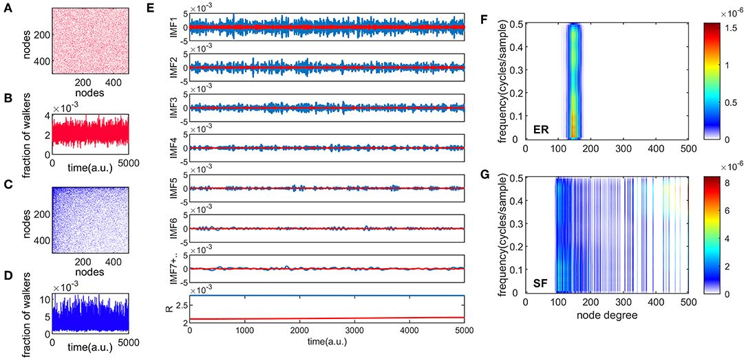
Figure 1. Different temporal modes of information flow in complex networks. Panels (A,C) are examples of ER and SF connectivity matrices, respectively, with N = 500 and e = 0.9. Panels (B,D) show one realization of the information flow in the network for 5000 time steps, for ER and SF networks, respectively. The total number of walkers present in each network was 10⁴. Panel (E) shows the empirical mode decomposition (EMD) of the time series in panels (B,D), producing different intrinsic mode functions (IMF), and a residue (R). This appears in red (blue) for the ER (SF) networks. Panels (F,G) show the spectrum of the random walk process organized by the node degree for ER and SF networks, respectively.

To characterize the interaction between frequencies, we computed three types of CFC interactions, PAC_kl, AAC_kl, and PPC_kl, between all possible combinations of the 7 IMFs (k = 1, 2, …, 7, l = 1, 2, …, 7, k > l, thus obtaining a 7 × 7 upper triangular matrix for each measure) for 3 different values of sparsity (e = [0.9, 0.8, 0.7]) of ER and SF networks (Figure 2). Figure 2 shows the average over K = 10⁴ realizations of PAC_kl (Figure 2A), AAC_kl (Figure 2B), and PPC_kl (Figure 2C) for ER and SF networks. Supplementary Figure 1 shows the corresponding Z-scores. In the case of PAC, Z-score values obtained for SF networks were higher than the corresponding values obtained in ER networks. Strong PAC values in SF networks involved the phase of IMF7 (the slowest IMF) and the amplitudes of IMF6 to IMF1. On the other hand, the highest AAC and PPC values in SF networks involved IMFs with close frequencies such as IMF1 and IMF2. In the case of ER networks, the strongest values were obtained for interactions between slow IMFs for PAC (phase of IMF7 and amplitude of IMF5 in Figure 2A), AAC (amplitudes of IMF7 and IMF6 in Figure 2B) and between fast IMFs for PPC (phases of IMF2 and IMF1 in Figure 2C). When we decreased the level of sparsity (i.e., the network became more connected), the results for SF networks turned similar to the ones in ER networks. In conclusion, PAC interactions in SF networks were the strongest CFC found (as reflected by the Z-scores) and, when compared to results from ER networks, the main difference was the existence of strong PAC between slow and fast oscillatory components of the information flow in the network.

FIGURE 2

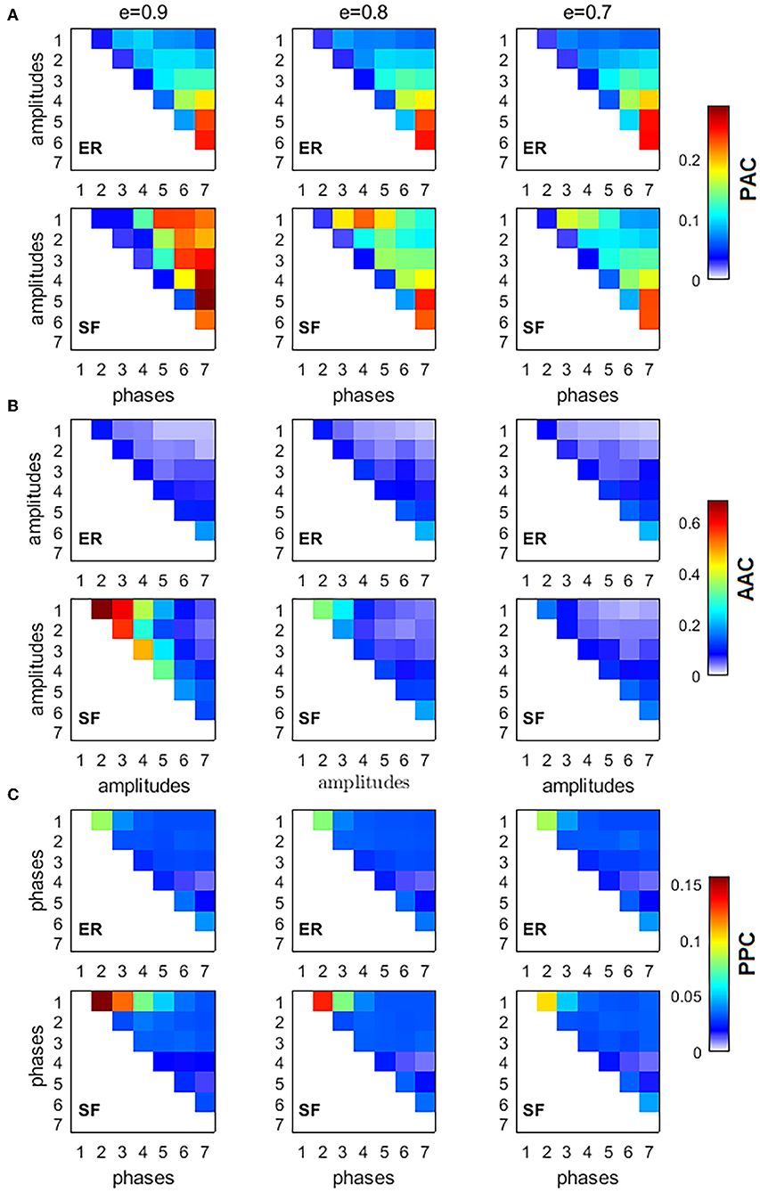
Figure 2. Cross-frequency interactions between the fundamental modes of information flow in ER and SF networks. All simulated networks had N = 500 nodes, and 10⁴ random walkers were placed over them, each performing 5, 000 time steps. Three different values of network sparsity were considered: e = [0.9, 0.8, 0.7]. (A) phase-amplitude coupling (PAC), (B) amplitude-amplitude coupling (AAC), (C) phase-phase coupling (PPC).

To verify our results were not an artifact of the application of the EMD method, we defined seven non-overlapping frequency bands (0.001–0.009, 0.010–0.020, 0.021–0.040, 0.041–0.060, 0.061–0.100, 0.101–0.250, and 0.251–0.490 cycles/sample) based on the seven IMFs and computed the CFC measures. Supplementary Figure 2 shows similar CFC patterns to the ones obtained for the Z-scores in Supplementary Figure 1, suggesting our results are not dependent on the EMD method but a consequence of the network architecture instead. Differences between the two figures are associated to the fact that consecutive IMFs have a small overlap in frequency by design [10].

We also studied the influence of specific nodes in the SF networks in the generation of PAC, AAC, and PPC. The contribution of each node i was computed by removing the node from the network and running the random walker analysis on the new network. The obtained PAC, AAC, and PPC were denoted as $PA{C}_i^r$, $AA{C}_i^r$, and $PP{C}_i^r$, respectively. The contribution of a node to the corresponding CFC measure is the change in the CFC value as a result of removing the node from the network: $\Delta PA{C}_i=|PA{C}_i^r/PAC-1|$, $\Delta AA{C}_i=|AA{C}_i^r/AAC-1|$, and $\Delta PP{C}_i=|PP{C}_i^r/PPC-1|$. Additionally, we computed several local topological properties for all nodes in the network using the Brain Connectivity Toolbox [38], namely: the degree (k); the efficiency (e), which quantifies a network's resistance to failure on a small scale; the clustering coefficient (cc), which measures the degree to which nodes in a graph tend to cluster together; assortativity (a), which indicates if a node tends to link to other nodes with the same or similar degree; betweenness centrality (bc), which is the fraction of shortest paths in the network that contain a given node (a node with higher betweenness centrality has more control over the network because more information will pass through it); eigenvector centrality (ec), which is another measure of centrality where relative scores are assigned to all nodes based on the concept that connections to high-scoring nodes contribute more to the score of the node in question than equal connections to low-scoring nodes; subgraph centrality (sc), which is a weighted sum of closed walks of different lengths in the network starting and ending at the node; and the product of the three centrality measures (ec × sc × bc). Figures 3A–C show the Pearson correlation between the eight topological measures and ΔPAC, ΔAAC, and ΔPPC, respectively. Different frequency combinations presented different correlation values. The strongest correlations involving ΔPAC were found for the topological measure composed by the product of the three centrality measures (ec × sc × bc), between the phase of IMF3 and the amplitude of IMF1. The amplitude of IMF1 was also involved in strong correlations with the phases of IMF4, IMF5, and IMF6. Of the three CFC measures, ΔAAC was most strongly correlated to topology (Figure 3B), specifically with centrality measures, followed by ΔPAC. ΔPPC was weakly correlated to the topology of the network.

FIGURE 3

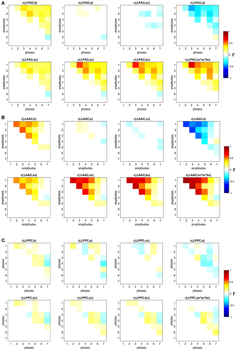
Figure 3. Correlation between changes in CFC and eight topological measures: degree (k), efficiency (e), clustering coefficient (cc), assortativity (a), eigenvector centrality (ec), subgraph centrality (sc), betweenness centrality (bc), product of three centrality measures (ec × sc × bc). Non-significant (p < 0.05) correlation values after correction by false-discovery rate are displayed in white (A) PAC, (B) AAC, (C) PPC.

Next, by using the degrees k we classified nodes in the network into hubs if their degree was at least one standard deviation above the network mean [39], and into non-hubs otherwise. We then computed the average ΔPAC of all frequency combinations involving the amplitudes of fast frequencies (IMF1 and IMF2) and the phases of slow frequencies (IMF5, IMF6, and IMF7). Note that the correlations between ΔPAC corresponding to these frequency combinations and the product ec × sc × bc are between 0.24 and 0.47 (Figure 3A), which suggests that other mechanisms are needed to explain these ΔPAC values.

Figure 4A plots ΔPAC vs. node degree for all nodes in the SF network. Interestingly, hubs, the most connected nodes in the network, are not necessarily involved in the largest ΔPAC values. Non-hubs were classified into three groups by equally dividing the ΔPAC range (0−0.6): bottom (0−0.2), middle (0.2−0.4), and top (0.4−0.6). The histogram in Figure 4B shows the probability that nodes in the four groups (hubs and three non-hubs groups) have of connecting to nodes of certain degrees. We see that top non-hubs connect to high degree nodes (hubs in Figure 4A) with higher probability than middle and bottom non-hubs. On the other hand, hubs connect with high probability to low degree nodes. Since PAC is defined as the coupling from a low to a high frequency, its highest contributor will be the nodes associated more with low frequencies (i.e., nodes with low degrees, see Figure 1G) and that also connect to nodes that are more associated to high frequencies (i.e., nodes with high degrees, see Figure 1G); that is, the top non-hubs. Accordingly, hubs, which are more connected to low frequency nodes contribute less to PAC, except for only one hub which presented the largest ΔPAC_i of all nodes in the network (Figures 1A,C,E). This hub (node with degree 270 in Figure 4) is known as a super-hub for having degree significantly higher than other hubs in the network [40]. Since the classification into top, middle, and bottom non-hubs based on ΔPAC values is somewhat arbitrary, we explored the results of changing the ΔPAC range of these three groups. Figures 4C,D show the results when the groups were defined by the bands: bottom (0−0.1), middle (0.1−0.5), and top (0.5−0.6). In this case, the number of nodes in the top and bottom groups were reduced and the probability that top non-hubs connected to high degree nodes increased.

FIGURE 4

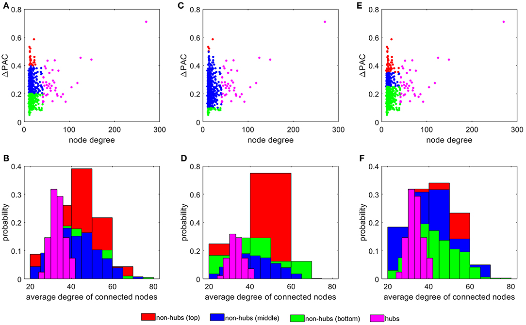
Figure 4. The influence of non-hubs vs. hubs on ΔPAC. Average ΔPAC for each node degree for three different grouping of non-hubs: (A) bottom (0 − 0.2), middle (0.2 − 0.4), and top (0.4 − 0.6), (C) bottom (0 − 0.1), middle (0.1 − 0.5), and top (0.5 − 0.6), and (E) bottom (0 − 0.25), middle (0.25 − 0.35), and top (0.35 − 0.6). Panels (B,D,F) present the probability of the four different groups of nodes of connecting to nodes of certain degrees, corresponding to the node distribution presented in panels (A,C,E), respectively.

In the calculations leading to Figure 4E we increased the number of nodes in the top and bottom groups as compared to Figure 4A by selecting the ranges: bottom (0 − 0.35), middle (0.35 − 0.45), and top (0.45 − 0.6). In this case, the probability for the top non-hubs decreased and the results for the top and middle groups were more similar (see Figure 4F).

Information Flow in Brain Networks Estimated From Healthy and Alzheimer's Disease Subject's Data

The information flow, as given by the movement of the random walkers, was also investigated in real brain networks. For this, freely available (http://adni.loni.usc.edu) images from ADNI were utilized and brain connectivity matrices for HC and AD subjects were computed. Figure 5A shows the connectivity matrix W for a representative HC subject. For each of the 44 HC subjects, we placed 10⁴ random walkers on top of its W and recorded a sequence of 5, 000 time steps.

FIGURE 5

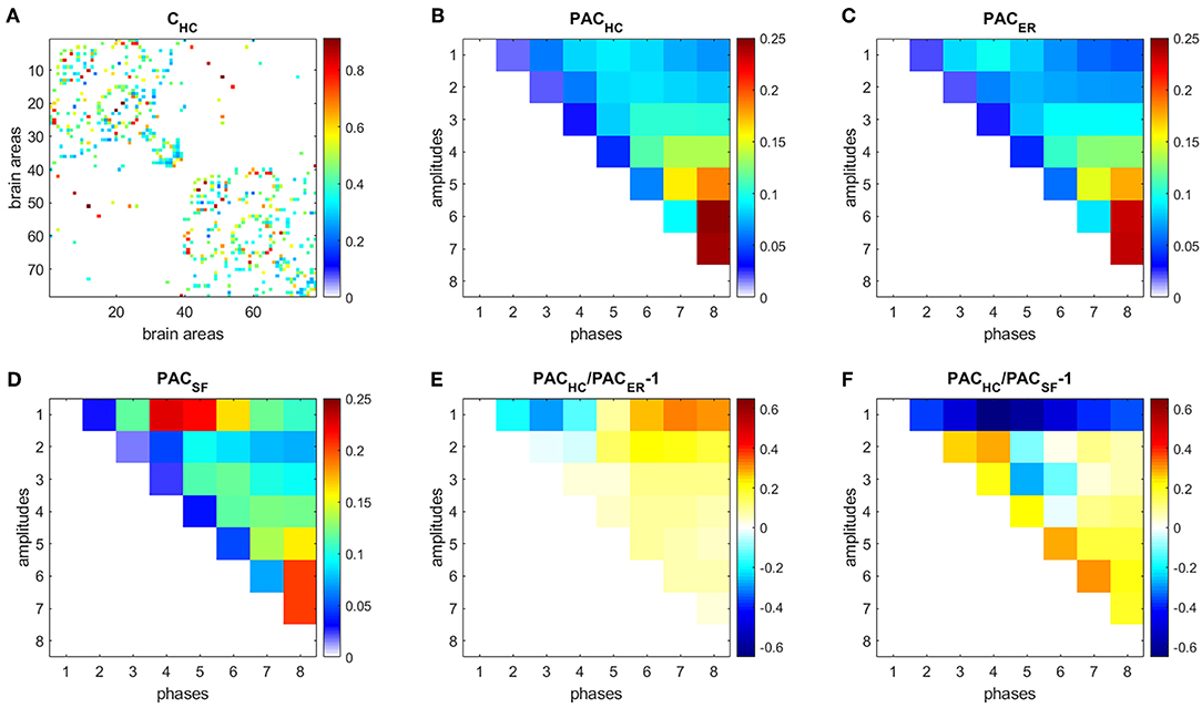
Figure 5. PAC in HC. (A) Connectivity matrix. (B) PAC averaged over 44 HC subjects. (C) Average PAC generated from 500 equivalent ER networks. (D) Average PAC generated from 500 equivalent SF networks. (E) Comparison of PAC from HC and PAC generated from equivalent ER networks. (F) Comparison of PAC from HC and PAC generated from equivalent SF networks.

Each time series was decomposed into 8 IMFs. We then focused on PAC since it was the strongest CFC type obtained for both ER and SF networks in our simulations (Supplementary Figure 1). Figure 5B shows the PAC between all possible combinations of the 8 IMFs, averaged over 10⁴ realizations and over the 44 HC subjects, denoted as PAC_HC. The strongest PAC values were obtained for interactions between slow IMFs (the phase of IMF8 and the amplitudes of IMF5, IMF6, and IMF7). Additionally, for each subject, we generated 500 ER and 500 SF networks of the same size and number of edges as their W matrices, computed PAC for these matrices and averaged the results, obtaining PAC_ER (Figure 5C), and PAC_SF (Figure 5D), respectively. We then computed the following measures: $\frac{PA{C}_{HC}}{PA{C}_{ER}}-1$ (Figure 5E), $\frac{PA{C}_{HC}}{PA{C}_{SF}}-1$ (Figure 5F). A similar analysis as in Figure 5, was performed to data from AD subjects and is shown in Figure 6.

FIGURE 6

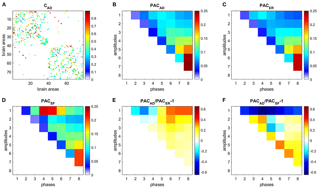
Figure 6. PAC in AD. (A) Connectivity matrix. (B) PAC averaged over 31 AD subjects. (C) Average PAC generated from 500 equivalent ER networks. (D) Average PAC generated from 500 equivalent SF networks. (E) Comparison of PAC from AD and PAC generated from equivalent ER networks. (F) Comparison of PAC from AD and PAC generated from equivalent SF networks.

Results for HC (Figure 5) and AD (Figure 6) show that interactions between phases of slow frequencies (IMF 5–8) and amplitudes of high frequencies (IMF1) are stronger in real brain networks than in simulated ER networks but weaker than in SF networks. This result is not surprising since we know that the degree distribution of brain anatomical networks do not follow a pure power law, as in SF networks, and is better described by an exponentially truncated power law [23].

We also compared HC and AD results (Figure 7). Figure 7A shows the difference between the average connectivity matrix of HC and AD subjects. The comparison between PAC in HC (Figure 5B) and AD (Figure 6B) shows that PAC between fast frequencies (IMF1) and slower modes (IMFs 3–8) weaken during AD as compared to HCs (see Figure 7B).

FIGURE 7

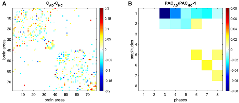
Figure 7. Comparing PAC in HC and AD subjects. (A) Difference between the average connectivity matrix of HC and AD subjects. (B) Comparison between PAC in HC and AD. Non-significant differences (p < 0.05) after correcting by false-discovery rate are displayed in white.

The contribution of each area to the generation of the PAC phenomenon (ΔPAC) was computed following the procedure described in the previous section. Figures 8A,B shows the average ΔPAC across subjects for the areas with the strongest influence on PAC, for the HC and AD groups, respectively. In both groups the two areas with the strongest influence were the right superior frontal followed by the right medial orbitofrontal. We also computed the measure $1-\frac{{PAC}_{AD}}{{PAC}_{HC}}$ to determine the areas that changed more between HC and AD. Figure 8C shows the areas for which the influence on PAC was stronger in HC than in AD, whereas Figure 8D displays the opposite case. We obtained that the influence of the right precentral and right superior parietal areas decreased in AD as compared to HC, whereas the influence of the right amygdala increased.

FIGURE 8

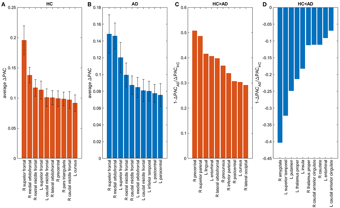
Figure 8. Influence of brain areas on PAC: areas that when removed from the network change PAC the most in HC (A), AD (B). Areas for which the change was larger in HC (AD) than in AD (HC) appear in panels (C,D). “L” and “R” denote left and right hemispheres, respectively.

We also extracted all possible shortest paths [38] in the HC and AD brain networks, and computed the average ΔPAC of the areas involved in those paths. We found that the ΔPAC pathway right superior frontal-right medial orbitofrontal-left superior frontal presented the strongest ΔPAC in both HC and AD groups (red path in Figure 9). On the other hand, the ΔPAC pathway that increased the most during AD was left insula-left pars opercularis-left superior temporal (green in Figure 9), whereas the PAC route that decreased the most in AD was right precentral-right paracentral-right precuneus (cyan in Figure 9). This clearly demonstrates an interhemispheric difference in PAC generation during AD.

FIGURE 9

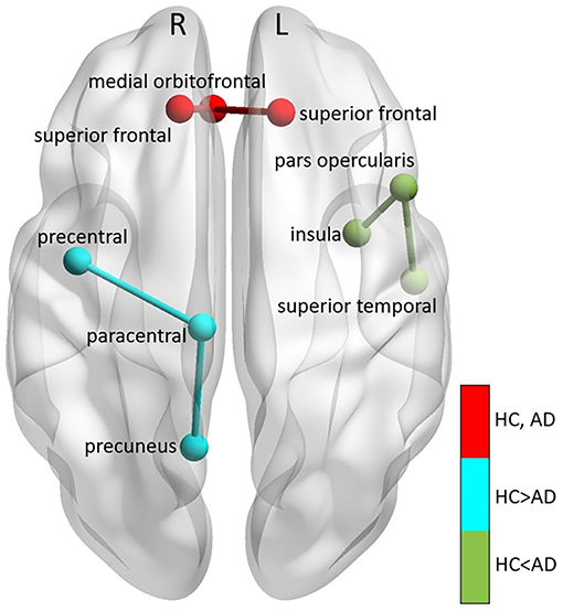
Figure 9. Main PAC paths in HC and AD. Three main paths were found: (1) right superior frontal-right medial or bitofrontal-left superior frontal corresponding to the strongest PAC in HC, remaining also the strongest in AD (colored in red), (2) left insula-left pars opercularis-left superior temporal, the path that decreased the most in AD compared to HC (colored in cyan), and (3) right precentral-right paracentral-right precuneus, which increased the most in AD compared to HC (colored in green). “L” and “R” denote left and right hemispheres, respectively.

Here, we also looked at how the scores of two customarily-used cognitive tests are related to the flow of information in AD networks as reflected by PAC. The individual clinical diagnoses assigned by the ADNI experts and used to define the HC and AD groups were based on multiple clinical evaluations [41]. The first test was the Clinical Dementia Rating Sum of Boxes (CDRSB), which provides a global rating of dementia severity through interviews on different aspects [41, 42]. An algorithm conduces to a score in each of the domain boxes, which are later summed. The final score ranges from 0 to 18, with a 0-value meaning “Normal.” CDRSB is a gold standard for the assessment of functional impairment [41]. The second test was the Functional Activities Questionnaire (FAQ), where an informant is asked to rate the subject's ability to perform 10 different activities of daily living [43]. The total score ranges from 0 (independent) to 30 (dependent).

For each brain area the linear fit between ΔPAC and CDRSB, and ΔPAC and FAQ was computed. Figure 10 shows the linear fits in the left y-axis (colored in blue) corresponding to the regions with the strongest correlations. For the case of CDRSB, the brain areas were left middle temporal (r = 0.61, p = 0.0005), left inferior temporal (r = 0.53, p = 0.004), and right middle temporal (r = 0.40, p = 0.032), whereas for the case of FAQ, the left middle temporal (r = 0.55, p = 0.002), left inferior temporal (r = 0.47, p = 0.011) were obtained again, with the appearance of the left pars orbitalis (r = 0.36, p = 0.056) among the top-three now.

FIGURE 10

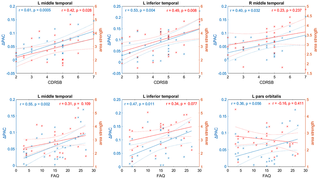
Figure 10. Relationship between two cognitive tests– CDRSB and FAQ– and PAC (in blue) and values of the node strength (in red) for selected areas of the AD networks. Solid and dashed lines represent the linear fit and confidence intervals, respectively.

We also performed a linear fit for the two cognitive test and the strength of each area (defined as the sum of all the connections associated with area $i,s_i=\sum _{j=1}^N{w}_{ij}$). The results are displayed in the right axis (colored in red) of every panel in Figure 10. We obtained the best fits for the same areas that resulted from using ΔPAC. The above-mentioned result is expected since PAC is obtained as a result of the movement of the random walkers on top of the matrices W. However, the correlation values obtained were smaller and statistically significant only in two out of the six cases: the CDRSB test with the strength of left middle temporal (r = 0.42, p = 0.0028) and left inferior temporal (r = 0.49, p = 0.008) areas. The correlation between CDRSB and the right middle temporal area (r = 0.23, p = 0.237) was not significant, and neither were the correlations between the three areas and the FAQ test: left middle temporal (r = 0.31, p = 0.109), left inferior temporal (r = 0.34, p = 0.077), left pars orbitalis (r = −0.16, p = 0.411). These results suggest the existence of a relationship between cognitive impairment, functional decline and behavioral symptoms that characterize AD and the perturbations to the information flow in brain networks, as characterized by cross-frequency interactions and not by broadband interactions (functional connectivity).

Discussion

In summary, we employed random walkers to sample the spatial structure of complex networks and converted their movement into time series. To estimate the different temporal scales, these time series were further decomposed into intrinsic mode functions, or IMFs by means of the EMD technique [10]. Expressed in IMFs, the temporal scales have well-behaved Hilbert transforms [10], from which the instantaneous phases and amplitudes can be calculated. Another advantage of using EMD is that it is an adaptive and data-driven method that does not require prior knowledge on the number of temporal modes embedded into the time series. The interaction between IMFs, or CFS, was analyzed, obtaining that cross-frequency interactions were stronger in SF than in ER networks, especially for the case of PAC. SF networks presented strong PAC between slow and high frequency components of the information flow, whereas ER networks presented the strongest PAC between slow-frequency components. Since EMD acts essentially as a dyadic filter bank [44], some overlapping between consecutive IMFs is expected, which can result in strong CFC. This phenomenon can be seen in Supplementary Figure 1 for the cases of PAC (interaction between the phase of IMF7 and the amplitude of IMF6), AAC (interaction between the amplitudes of IMF2 and IMF1), and PPC (interaction between the phases of IMF2 and IMF1). When filtering the data using non-overlapping bands (Supplementary Figure 2) the strength of these couplings decreased, but the CFC patterns, specifically the strong PAC connection between slow phases (IMFs 5–7) and fast frequencies (IMF1), was preserved, supporting the use of EMD in our analysis.

The temporal architectures of complex networks, and specifically of the human brain, have been topics of increasing interest in the past decade [45]. Dynamic functional connectivity studies have demonstrated that brain networks are not stationary but fluctuate over time [46, 47]. To study these dynamic networks, multi-layer network models are commonly employed [48–50]. These models treat the network at each time point as a layer [51]. Alternatively, each layer in the multi-layer network can be linked to a different frequency component [52]. The multi-layer network framework have been used to study the cross-frequency interactions in functional networks estimated from magnetoencephalographic (MEG) data [49]. However, these studies did not establish a link between the multiplex network and the information flow in the brain. This has been done recently for general multilayer networks by means of the so-called directed information measure [53], although cross-frequency interactions were not analyzed [54].

Given a complex network, it is of interest to determine which nodes contribute the most to CFC. We studied in more detail the generation of PAC between low (IMFs 5–7) and high (IMF1) frequencies and found that hubs, the most connected nodes in the network were not involved in the strongest PAC [with the exception of one super-hub [40]]. The most significant influence on PAC was exerted by a group of non-hubs, which connected with high probability to high degree nodes (Figure 4). This facilitated the generation of PAC [information flow from low to high frequencies [11]] since low and high degree nodes were generally associated with low and high frequencies, respectively. Our results are in agreement with recent work [55] studying the dynamic patterns of information flow in complex networks by means of a perturbative method. Interestingly, the authors found that the information flow preferred non-hubs and avoided centralized pathways. However, their study only reflected the broadband flow phenomena, i.e., unspecific and ignoring frequency interactions, unlike this work.

We applied our methodology to brain networks from HC subjects and AD patients and found that PAC activity between slow frequencies and IMF1 decreased during AD. The IMFs obtained from simulated ER and SF networks correspond to different oscillatory modes, with normalized frequencies (Figures 1F,G). In the case of brain networks, it is tempting to analyze the frequencies in Hz, in order to compare the frequency range of the different IMFs to the known frequency bands registered in the human brain. For this, we need to know the conduction delays for signals coming from different brain areas. Delays can range from a few milliseconds to several hundreds of milliseconds depending on the regions involved and the species considered [56–58]. Unfortunately, for the human brain, there is lack of information about conduction delays between all the combinations of areas, which makes the conversion to frequency units unfeasible at this time.

When analyzing the influence of specific brain areas, we found the right superior frontal and the right medial frontal to be the areas that contributed more to PAC in both HC and AD subjects. These areas belong to the default mode network (DMN), a collection of brain structures which intertwined activity increases in the absence of a task and has been associated with memory consolidation. The right superior frontal and the right medial frontal are also involved in the strongest PAC-based information flow pathway found in AD and HC: right superior frontal-right medial orbitofrontal-left superior frontal. The DMN is of interest to AD research given the amyloid deposits found in its regions [59, 60]. We also found that the influence of the right amygdala on PAC increased during AD (Figure 6D); the amygdala is known to be severely affected in AD [61].

Our results also demonstrated a marked interhemispheric difference in the generation of PAC, with areas within the left hemisphere being more correlated to the cognitive scores (Figure 8). Furthermore, the PAC pathway that decreased the most during AD consisted of left hemisphere areas only (left insula-left pars opercularis-left superior temporal), whereas the PAC pathway that increased the most in AD was formed by areas from the right hemisphere (right precentral-right paracentral-right precuneus). A tentative explanation is that the brain must enhance traffic over this specific pathway we have obtained to maintain at least a minimal information flow on the right hemisphere in AD. The interhemispheric functional disconnection suggested by our results has been previously reported in mild cognitive impairment and AD subjects [62–64], and has been associated with white matter degeneration [64].

One important challenge for the AD research field is the development of efficient biomarkers. Neuroimaging biomarkers in AD are based on brain signals such as MRI, fMRI, and Positron Emission Tomography (PET). For instance, there is a consistently reported decrease in resting-state functional connectivity in AD patients compared to HCs in the DMN [65]. However, when we correlated the strength of functional connections with the reported scores of two different cognitive tests usually employed to diagnose AD, only two areas (both from the DMN), the left middle temporal and left inferior temporal presented significant correlations (0.42 and 0.49, respectively, with p < 0.05) with one of the tests, the CDRSB. On the other hand, these two same areas presented significant and stronger correlations between PAC and both tests, the CDRSB (r = 0.61, r = 0.53) and FAQ (r = 0.55, r = 0.47). Additionally, the right middle temporal PAC presented a significant correlation (r = 0.40) with the CDRSB scores. These findings suggest that our PAC-based analysis could be more sensitive to network changes induced by AD, when compared to the traditional utilization of functional connectivity values. Thus, there exists a potentially elevated clinical value of PAC as a useful biomarker for the disease. These results support the feasibility of translating network properties into functional predictions.

A limitation of our brain networks analysis was the use of the backbone obtained from HC subjects for the AD patients. By using the same backbone matrix, we assumed that the propagation of information at the large-scale via white matter fiber connections is approximately the same for both HC and AD. This assumption is supported by past studies that found that misfolded proteins deposition and structural atrophy patterns in neurodegeneration match with the structural and functional connectome patterns obtained for young healthy subjects [3, 66, 67]. Furthermore, a recent study [68] found that despite changes in the integrity of specific fiber tracts, white matter organization in AD is preserved, suggesting AD does not appear to alter the ability of the anatomical network to mediate pathology spread in AD. However, this is in contrast to prior reports of significant changes in network topology in AD vs. HC [69, 70]. These discrepancies have been attributed to dissimilar methodologies in the network construction such as edge thresholding, binarization, and inclusion of subcortical regions to network graphs [68]. In this paper, we have considered differences between the two groups in terms of the functional matrices only and acknowledge that some bias given by the anatomical backbone may exist.

Data Availability

All MRI and fMRI data used in this study were obtained from the Alzheimer's Disease Neuroimaging Initiative (ADNI) database (http://adni.loni.usc.edu). For researchers who meet the criteria for access to the data; access to the ADNI data is available through an online application, which can be submitted at the following link: http://adni.loni.usc.edu/data-samples/access-data/.

Ethics Statement

Data used in this article were obtained from the Alzheimer's Disease Neuroimaging Initiative (ADNI) database (adni.loni.usc.edu). The ADNI study was conducted according to Good Clinical Practice guidelines, the Declaration of Helsinki Principles, US 21CFR Part 50-Protection of Human Subjects, and Part 56-Institutional Review Boards, and pursuant to state and federal HIPAA regulations (adni.loni.usc.edu). Study subjects and/or authorized representatives gave written informed consent at the time of enrollment for sample collection and completed questionnaires approved by each participating sites Institutional Review Board.

Author Contributions

RS conceived the project. RS, LS-R, MD, YI-M, and JS-B assisted with analysis and interpretation of data, and with writing and editing of the manuscript.

Funding

This work was partially supported by grant RGPIN-2015-05966 from the Natural Sciences and Engineering Research Council of Canada. Data collection and sharing for this project was funded by the Alzheimer's Disease Neuroimaging Initiative (ADNI) (National Institutes of Health Grant U01 AG024904) and DOD ADNI (Department of Defense award number W81XWH-12-2-0012). ADNI is funded by the National Institute on Aging, the National Institute of Biomedical Imaging and Bioengineering, and through generous contributions from the following: AbbVie, Alzheimer's Association; Alzheimer's Drug Discovery Foundation; Araclon Biotech; BioClinica, Inc.; Biogen; Bristol-Myers Squibb Company; CereSpir, Inc.; Eisai Inc.; Elan Pharmaceuticals, Inc.; Eli Lilly and Company; EuroImmun; F. Hoffmann-La Roche Ltd. and its affiliated company Genentech, Inc.; Fujirebio; GE Healthcare; IXICO Ltd.; Janssen Alzheimer Immunotherapy Research & Development, LLC.; Johnson & Johnson Pharmaceutical Research & Development LLC.; Lumosity; Lundbeck; Merck and Co., Inc.; Meso Scale Diagnostics, LLC.; NeuroRx Research; Neurotrack Technologies; Novartis Pharmaceuticals Corporation; Pfizer Inc.; Piramal Imaging; Servier; Takeda Pharmaceutical Company; and Transition Therapeutics. The Canadian Institutes of Health Research is providing funds to support ADNI clinical sites in Canada. Private sector contributions are facilitated by the Foundation for the National Institutes of Health (www.fnih.org). The grantee organization is the Northern California Institute for Research and Education, and the study is coordinated by the Alzheimer's Disease Cooperative Study at the University of California, San Diego. ADNI data are disseminated by the Laboratory for Neuro Imaging at the University of Southern California.

Conflict of Interest Statement

The authors declare that the research was conducted in the absence of any commercial or financial relationships that could be construed as a potential conflict of interest.

Supplementary Material

The Supplementary Material for this article can be found online at: https://www.frontiersin.org/articles/10.3389/fphy.2019.00107/full#supplementary-material

References

1. Gallos LK, Song C, Havlin S, Makse HA. Scaling theory of transport in complex biological networks. Proc Natl Acad Sci USA. (2007) 104:7746–51. doi: 10.1073/pnas.0700250104

PubMed Abstract | CrossRef Full Text | Google Scholar

2. Gfeller D, De Los Rios P, Caflisch A, Rao F. Complex network analysis of free-energy landscapes. Proc Natl Acad Sci USA. (2007) 104:1817–22. doi: 10.1073/pnas.0608099104

PubMed Abstract | CrossRef Full Text | Google Scholar

3. Raj A, Kuceyeski A, Weiner M. A network diffusion model of disease progression in dementia. Neuron. (2012) 73:1204–15. doi: 10.1016/j.neuron.2011.12.040

PubMed Abstract | CrossRef Full Text | Google Scholar

4. Simonsen I, Astrup Eriksen K, Maslov S, Sneppen K. Diffusion on complex networks: a way to probe their large-scale topological structures. Physica A. (2004) 336:163–73. doi: 10.1016/j.physa.2004.01.021

CrossRef Full Text | Google Scholar

5. Pearson K. The problem of the random walk. Nature. (1905) 72:294. doi: 10.1038/072294b0

CrossRef Full Text | Google Scholar

6. Bonaventura M, Nicosia V, Latora V. Characteristic times of biased random walks on complex networks. Phys Rev E. (2014) 89:012803. doi: 10.1103/PhysRevE.89.012803

PubMed Abstract | CrossRef Full Text | Google Scholar

7. Noh JD, Rieger H. Random walks on complex networks. Phys Rev Lett. (2004) 92:118701. doi: 10.1103/PhysRevLett.92.118701

PubMed Abstract | CrossRef Full Text | Google Scholar

8. Noskowicz SH, Goldhirsch I. First-passage-time distribution in a random walk. Phys Rev A. (1990) 42:2047–64. doi: 10.1103/PhysRevA.42.2047

PubMed Abstract | CrossRef Full Text | Google Scholar

9. Tejedor V, Bénichou O, Voituriez R. Global mean first-passage times of random walks on complex networks. Phys Rev E. (2009) 80:065104. doi: 10.1103/PhysRevE.80.065104

PubMed Abstract | CrossRef Full Text | Google Scholar

10. Huang NE, Shen Z, Long SR, Wu MC, Shih HH, Zheng Q, et al. The empirical mode decomposition and the Hilbert spectrum for nonlinear and non-stationary time series analysis. Proc R Soc A Math Phys Eng Sci. (1998) 454:903–95. doi: 10.1098/rspa.1998.0193

CrossRef Full Text | Google Scholar

11. Sotero RC. Topology, cross-frequency, and same-frequency band interactions shape the generation of phase-amplitude coupling in a neural mass model of a cortical column. PLoS Comput Biol. (2016) 12:e1005180. doi: 10.1371/journal.pcbi.1005180

PubMed Abstract | CrossRef Full Text | Google Scholar

12. Sotero RC. Modeling the generation of phase-amplitude coupling in cortical circuits: from detailed networks to neural mass models. Biomed Res Int. (2015) 2015:1–12. doi: 10.1155/2015/915606

PubMed Abstract | CrossRef Full Text | Google Scholar

13. Bruns A, Eckhorn R. Task-related coupling from high- to low-frequency signals among visual cortical areas in human subdural recordings. Int J Psychophysiol. (2004) 51:97–116. doi: 10.1016/j.ijpsycho.2003.07.001

PubMed Abstract | CrossRef Full Text | Google Scholar

14. Lachaux J-P, Rodriguez E, Martinerie J, Varela FJ. Measuring phase synchrony in brain signals. Hum Brain Mapp. (1999) 8:194–208. doi: 10.1002/(SICI)1097-0193(1999)8:4<194::AID-HBM4>3.0.CO;2-C

PubMed Abstract | CrossRef Full Text | Google Scholar

15. Erdös P, Rényi A. On random graphs, I. Debrecen: Publicationes Mathematicae, 6 (1959).

16. Barabasi A-L, Albert R. Emergence of scaling in random networks. Science. (1999) 286:509–12. doi: 10.1126/science.286.5439.509

PubMed Abstract | CrossRef Full Text | Google Scholar

17. Barrat A, Barthelemy M, Vespignani A. Dynamical Processes on Complex Networks. Cambridge: Cambridge University Press. (2008). doi: 10.1017/CBO9780511791383

CrossRef Full Text | Google Scholar

18. Taylor A, Higham DJ. CONTEST. ACM Trans Math Softw. (2009) 35:1–17. doi: 10.1145/1462173.1462175

CrossRef Full Text | Google Scholar

19. Sled JG, Zijdenbos AP, Evans AC. A nonparametric method for automatic correction of intensity nonuniformity in MRI data. IEEE Trans Med Imaging. (1998) 17:87–97. doi: 10.1109/42.668698

PubMed Abstract | CrossRef Full Text | Google Scholar

20. Evans AC, Kamber M, Collins DL, MacDonald D. An MRI-based probabilistic atlas of neuroanatomy. In: Shorvon SD, Fish DR, Andermann F, Bydder GM, Stefan H, editors. Magnetic Resonance Scanning and Epilepsy. Boston, MA: Springer US (1994). p. 263–74. doi: 10.1007/978-1-4615-2546-2_48

CrossRef Full Text | Google Scholar

21. Ashburner J. A fast diffeomorphic image registration algorithm. Neuroimage. (2007) 38:95–113. doi: 10.1016/j.neuroimage.2007.07.007

PubMed Abstract | CrossRef Full Text | Google Scholar

22. Klein A, Tourville J. 101 labeled brain images and a consistent human cortical labeling protocol. Front Neurosci. (2012) 6:171. doi: 10.3389/fnins.2012.00171

PubMed Abstract | CrossRef Full Text | Google Scholar

23. Iturria-Medina Y, Sotero RC, Canales-Rodriguez EJ, Aleman-Gomez Y, Melie-Garcia L. Studying the human brain anatomical network via diffusion-weighted MRI and Graph Theory. Neuroimage. (2008) 40:1064–76. doi: 10.1016/j.neuroimage.2007.10.060

PubMed Abstract | CrossRef Full Text | Google Scholar

24. Tournier J-D, Yeh C-H, Calamante F, Cho K-H, Connelly A, Lin C-P. Resolving crossing fibres using constrained spherical deconvolution: validation using diffusion-weighted imaging phantom data. Neuroimage. (2008) 42:617–25. doi: 10.1016/j.neuroimage.2008.05.002

PubMed Abstract | CrossRef Full Text | Google Scholar

25. Sotero RC, Trujillo-Barreto NJ, Iturria-Medina Y, Carbonell F, Jimenez JC. Realistically coupled neural mass models can generate EEG Rhythms. Neural Comput. (2007) 19:478–512. doi: 10.1162/neco.2007.19.2.478

PubMed Abstract | CrossRef Full Text | Google Scholar

26. Hagmann P, Cammoun L, Gigandet X, Meuli R, Honey CJ, Wedeen VJ, et al. Mapping the structural core of human cerebral cortex. PLoS Biol. (2008) 6:e159. doi: 10.1371/journal.pbio.0060159

PubMed Abstract | CrossRef Full Text | Google Scholar

27. Young MP. The organization of neural systems in the primate cerebral cortex. Proc R Soc London Ser B Biol Sci. (1993) 252:13–8. doi: 10.1098/rspb.1993.0040

PubMed Abstract | CrossRef Full Text | Google Scholar

28. Yan C, Zang Y. DPARSF: a MATLAB toolbox for “pipeline” data analysis of resting-state fMRI. Front Syst Neurosci. (2010) 4:13. doi: 10.3389/fnsys.2010.00013

CrossRef Full Text | Google Scholar

29. Cao J, Wang X, Liu H, Alexandrakis G. Directional changes in information flow between human brain cortical regions after application of anodal transcranial direct current stimulation (tDCS) over Broca's area. Biomed Opt Express. (2018) 9:5296–317. doi: 10.1364/BOE.9.005296

PubMed Abstract | CrossRef Full Text | Google Scholar

30. Yanagawa T, Chao ZC, Hasegawa N, Fujii N. Large-scale information flow in conscious and unconscious states: an ECoG study in monkeys. PLoS ONE. (2013) 8:e80845. doi: 10.1371/journal.pone.0080845

PubMed Abstract | CrossRef Full Text | Google Scholar

31. Zhang Z, Shan T, Chen G. Random walks on weighted networks. Phys Rev E. (2013) 87:012112. doi: 10.1103/PhysRevE.87.012112

CrossRef Full Text | Google Scholar

32. Wu Z, Huang NE. Ensemble empirical mode decomposition: a noise-assisted data analysis method. Adv Adapt Data Anal. (2009) 01:1–41. doi: 10.1142/S1793536909000047

CrossRef Full Text | Google Scholar

33. Colominas MA, Schlotthauer G, Torres ME. Improved complete ensemble EMD: a suitable tool for biomedical signal processing. Biomed Signal Process Control. (2014) 14:19–29. doi: 10.1016/j.bspc.2014.06.009

CrossRef Full Text | Google Scholar

34. Sotero RC, Bortel A, Naaman S, Mocanu VM, Kropf P, Villeneuve M, et al. Laminar distribution of phase-amplitude coupling of spontaneous current sources and sinks. Front Neurosci. (2015) 9:454. doi: 10.3389/fnins.2015.00454

PubMed Abstract | CrossRef Full Text | Google Scholar

35. van Driel J, Cox R, Cohen MX. Phase-clustering bias in phase–amplitude cross-frequency coupling and its removal. J Neurosci Methods. (2015) 254:60–72. doi: 10.1016/j.jneumeth.2015.07.014

PubMed Abstract | CrossRef Full Text | Google Scholar

36. Tass P, Rosenblum MG, Weule J, Kurths J, Pikovsky A, Volkmann J, et al. Detection of n : m phase locking from noisy data: application to magnetoencephalography. Phys Rev Lett. (1998) 81:3291–4. doi: 10.1103/PhysRevLett.81.3291

CrossRef Full Text | Google Scholar

37. Benjamini Y, Hochberg Y. Controlling the false discovery rate: a practical and powerful approach to multiple testing. J R Stat Soc Ser B. (1995) 57:289–300. doi: 10.1111/j.2517-6161.1995.tb02031.x

CrossRef Full Text | Google Scholar

38. Rubinov M, Sporns O. Complex network measures of brain connectivity: uses and interpretations. Neuroimage. (2010) 52:1059–69. doi: 10.1016/j.neuroimage.2009.10.003

PubMed Abstract | CrossRef Full Text | Google Scholar

39. Sporns O, Honey CJ, Kötter R. Identification and classification of hubs in brain networks. PLoS ONE. (2007) 2:e1049. doi: 10.1371/journal.pone.0001049

PubMed Abstract | CrossRef Full Text | Google Scholar

40. Hao D, Ren C, Li C. Revisiting the variation of clustering coefficient of biological networks suggests new modular structure. BMC Syst Biol. (2012) 6:34. doi: 10.1186/1752-0509-6-34

PubMed Abstract | CrossRef Full Text | Google Scholar

41. Defina PA, Moser RS, Glenn M, Lichtenstein JD, Fellus J. Alzheimer's disease clinical and research update for health care practitioners. J Aging Res. (2013) 2013:207178. doi: 10.1155/2013/207178

PubMed Abstract | CrossRef Full Text | Google Scholar

42. Doody RS, Pavlik V, Massman P, Rountree S, Darby E, Chan W. Predicting progression of Alzheimer's disease. Alzheimers Res Ther. (2010) 2:2. doi: 10.1186/alzrt25

CrossRef Full Text | Google Scholar

43. Juva K, Mäkelä M, Erkinjuntti T, Sulkava R, Ylikoski R, Valvanne J, et al. Functional assessment scales in detecting dementia. Age Ageing. (1997) 26:393–400. doi: 10.1093/ageing/26.5.393

PubMed Abstract | CrossRef Full Text | Google Scholar

44. Flandrin P, Rilling G, Goncalves P. Empirical mode decomposition as a filter bank. IEEE Signal Process Lett. (2004) 11:112–4. doi: 10.1109/LSP.2003.821662

CrossRef Full Text | Google Scholar

45. Betzel RF, Bassett DS. Multi-scale brain networks. Neuroimage. (2017) 160:73–83. doi: 10.1016/j.neuroimage.2016.11.006

PubMed Abstract | CrossRef Full Text | Google Scholar

46. Kundu S, Ming J, Pierce J, McDowell J, Guo Y. Estimating dynamic brain functional networks using multi-subject fMRI data. Neuroimage. (2018) 183:635–49. doi: 10.1016/j.neuroimage.2018.07.045

PubMed Abstract | CrossRef Full Text | Google Scholar

47. Li X, Zang Y-F, Zhang H. Exploring dynamic brain functional networks using continuous “state-related” functional MRI. Biomed Res Int. (2015) 2015:1–8. doi: 10.1155/2015/824710

PubMed Abstract | CrossRef Full Text | Google Scholar

48. Battiston F, Nicosia V, Chavez M, Latora V. Multilayer motif analysis of brain networks. Chaos. (2017) 27:047404. doi: 10.1063/1.4979282

PubMed Abstract | CrossRef Full Text | Google Scholar

49. Brookes MJ, Tewarie PK, Hunt BAE, Robson SE, Gascoyne LE, Liddle EB, et al. A multi-layer network approach to MEG connectivity analysis. Neuroimage. (2016) 132:425–38. doi: 10.1016/j.neuroimage.2016.02.045

PubMed Abstract | CrossRef Full Text | Google Scholar

50. Tewarie P, Hillebrand A, van Dijk BW, Stam CJ, O'Neill GC, Van Mieghem P, et al. Integrating cross-frequency and within band functional networks in resting-state MEG: a multi-layer network approach. Neuroimage. (2016) 142:324–36. doi: 10.1016/j.neuroimage.2016.07.057

PubMed Abstract | CrossRef Full Text | Google Scholar

51. De Domenico M, Solé-Ribalta A, Cozzo E, Kivelä M, Moreno Y, Porter MA, et al. Mathematical formulation of multilayer networks. Phys Rev X. (2013) 3:041022. doi: 10.1103/PhysRevX.3.041022

CrossRef Full Text | Google Scholar

52. De Domenico M, Sasai S, Arenas A. Mapping multiplex hubs in human functional brain networks. Front Neurosci. (2016) 10:326. doi: 10.3389/fnins.2016.00326

PubMed Abstract | CrossRef Full Text | Google Scholar

53. Kontoyiannis I, Skoularidou M. Estimating the directed information and testing for causality. IEEE Trans Inf Theory. (2016) 62:6053–67. doi: 10.1109/TIT.2016.2604842

CrossRef Full Text | Google Scholar

54. Guler B, Yener A, Swami A. Learning causal information flow structures in multi-layer networks. In: 2016 IEEE Global Conference on Signal and Information Processing (GlobalSIP). Washington, DC: IEEE (2016). p. 1340–4. doi: 10.1109/GlobalSIP.2016.7906059

CrossRef Full Text | Google Scholar

55. Harush U, Barzel B. Dynamic patterns of information flow in complex networks. Nat Commun. (2017) 8:2181. doi: 10.1038/s41467-017-01916-3

PubMed Abstract | CrossRef Full Text | Google Scholar

56. Aboitiz F, López J, Montiel J. Long distance communication in the human brain: timing constraints for inter-hemispheric synchrony and the origin of brain lateralization. Biol Res. (2003) 36:89–99. doi: 10.4067/S0716-97602003000100007

PubMed Abstract | CrossRef Full Text | Google Scholar

57. Budd JML, Kisvárday ZF. Communication and wiring in the cortical connectome. Front Neuroanat. (2012) 6:42. doi: 10.3389/fnana.2012.00042

PubMed Abstract | CrossRef Full Text | Google Scholar

58. Stoelzel CR, Bereshpolova Y, Alonso J-M, Swadlow HA. Axonal conduction delays, brain state, and corticogeniculate communication. J Neurosci. (2017) 37:6342–58. doi: 10.1523/JNEUROSCI.0444-17.2017

PubMed Abstract | CrossRef Full Text | Google Scholar

59. Sheline YI, Raichle ME, Snyder AZ, Morris JC, Head D, Wang S, et al. Amyloid plaques disrupt resting state default mode network connectivity in cognitively normal elderly. Biol Psychiatry. (2010) 67:584–7. doi: 10.1016/j.biopsych.2009.08.024

PubMed Abstract | CrossRef Full Text | Google Scholar

60. Sperling RA, Laviolette PS, O'Keefe K, O'Brien J, Rentz DM, Pihlajamaki M, et al. Amyloid deposition is associated with impaired default network function in older persons without dementia. Neuron. (2009) 63:178–88. doi: 10.1016/j.neuron.2009.07.003

PubMed Abstract | CrossRef Full Text | Google Scholar

61. Poulin SP, Dautoff R, Morris JC, Feldman Barrett L, Dickerson BC. Amygdala atrophy is prominent in early Alzheimer's disease and relates to symptom severity on behalf of the Alzheimer's Disease Neuroimaging Initiative. Psychiatry Res. (2011) 194:7–13. doi: 10.1016/j.pscychresns.2011.06.014

CrossRef Full Text | Google Scholar

62. Korolev I, Bozoki A, Majumdar S, Berger K, Zhu D. Alzheimer's disease reduces inter-hemispheric hippocampal functional connectivity. Alzheimers Dementia. (2011) 7:S739. doi: 10.1016/j.jalz.2011.05.2125

CrossRef Full Text | Google Scholar

63. Qiu Y, Liu S, Hilal S, Loke YM, Ikram MK, Xu X, et al. Inter-hemispheric functional dysconnectivity mediates the association of corpus callosum degeneration with memory impairment in AD and amnestic MCI. Sci Rep. (2016) 6:32573. doi: 10.1038/srep32573

PubMed Abstract | CrossRef Full Text | Google Scholar

64. Wang Z, Wang J, Zhang H, Mchugh R, Sun X, Li K, et al. Interhemispheric functional and structural disconnection in Alzheimer's disease: a combined resting-state fMRI and DTI study. PLoS ONE. (2015) 10:e0126310. doi: 10.1371/journal.pone.0126310

PubMed Abstract | CrossRef Full Text | Google Scholar

65. Dennis EL, Thompson PM. Functional brain connectivity using fMRI in aging and Alzheimer's disease. Neuropsychol Rev. (2014) 24:49–62. doi: 10.1007/s11065-014-9249-6

PubMed Abstract | CrossRef Full Text | Google Scholar

66. Iturria-Medina Y, Sotero RC, Toussaint PJ, Evans AC, Alzheimer's Disease Neuroimaging I. Epidemic spreading model to characterize misfolded proteins propagation in aging and associated neurodegenerative disorders. PLoS Comput Biol. (2014) 10:e1003956. doi: 10.1371/journal.pcbi.1003956

PubMed Abstract | CrossRef Full Text | Google Scholar

67. Zeighami Y, Ulla M, Iturria-Medina Y, Dadar M, Zhang Y, Larcher KM-H, et al. Network structure of brain atrophy in de novo Parkinson's disease. ELife. (2015) 4:1–20. doi: 10.7554/eLife.08440

PubMed Abstract | CrossRef Full Text | Google Scholar

68. Powell F, Tosun D, Sadeghi R, Weiner M, Raj A. Preserved structural network organization mediates pathology spread in Alzheimer's disease spectrum despite loss of white matter tract integrity. J Alzheimers Dis. (2018) 65:747–64. doi: 10.3233/JAD-170798

PubMed Abstract | CrossRef Full Text | Google Scholar

69. Daianu M, Jahanshad N, Nir TM, Toga AW, Jack CR, Weiner MW, et al. Breakdown of brain connectivity between normal aging and Alzheimer's disease: a structural k -core network analysis. Brain Connect. (2013) 3:407–22. doi: 10.1089/brain.2012.0137

PubMed Abstract | CrossRef Full Text | Google Scholar

70. Prescott JW, Guidon A, Doraiswamy PM, Roy Choudhury K, Liu C, Petrella JR, et al. The Alzheimer structural connectome: changes in cortical network topology with increased amyloid plaque burden. Radiology. (2014) 273:175–84. doi: 10.1148/radiol.14132593

PubMed Abstract | CrossRef Full Text | Google Scholar