Transient Anomalous Diffusion in Run-and-Tumble Dynamics

1. Introduction

Many transport processes in nature involve distinct motility states. Of particular interest is the run-and-tumble process, which consists of alternating phases of fast active and slow passive motion. Prominent examples are bacterial species that swim when their flagella form a bundle and synchronize their rotation. The bundle is disrupted and swimming stops when some of the flagella stochastically change their rotational direction. In the absence of rotating bundle, the bacterium moves diffusively until it manages to re-form the bundle and actively move forward again [1, 2]. The run-and-tumble dynamics is beneficial for bacteria as it allows them to react to the environmental changes by adjusting their average run time or speed [3], change their direction of motion, perform an efficient search [4–7], or optimize their navigation [8, 9].

Another example is the motion of molecular motors along cytoskeletal filaments. When motor proteins bind to filaments, they perform a number of steps until they randomly unbind and experience diffusion in the crowded cytoplasm. While the efficiency of long-distance cargo delivery requires high motor processivity (i.e., the tendency to continue the motion along the filament), the slow diffusive mode during unbinding periods is also vital for cellular functions which depend on the localization of the reactants [10–13]. The processivity of the motors (and thus the unbinding probability) depends on the type of motor and filament [14, 15] and the presence of particular proteins or binding domains in the surrounding medium [16–18]. On the other hand other factors, such as cell crowding, may affect the binding probability. Therefore, the switching probabilities between active run and tumble states are generally asymmetric. By ignoring the microscopic details of stepping on filaments, coarse-grained random walk models have been employed to study the two-state dynamics of molecular motors [19–22]. Dentritic immune cells also move persistently (migration phase) interrupted by slow phases for antigen uptake [23]. There have been many other locomotive patterns in biological and non-living systems investigated via models with distinct states of motility [24–33]. For instance, the problem of searcher proteins finding a specific target site over a DNA strand has been studied by multi-state stochastic processes [34–36].

The particle trajectories obtained from experiments often comprise a set of recorded positions of the particle, from which the successive directions of motion can be deduced. These directions are correlated on short time scales for active motions. However, the trajectory eventually gets randomized and the asymptotic dynamics is diffusive, with a diffusion constant D_asymp that depends on the particle velocity and persistency [37, 38]. One expects a similar long-term behavior for a mixture of run and tumble dynamics as well. The question arises how the transient short time dynamics, the crossover time to asymptotic diffusion, and D_asymp depend on the run and tumble velocities and the switching probabilities between the two states. It is also unclear how the overall dynamics is influenced by the choice of the initial conditions, like the probabilities to start either in the run or tumble state, which are parameters that can be extracted from experimental data.

Here, we present a two-state model for the run-and-tumble dynamics with spontaneous switchings between the states of motility. By deriving an analytical expression for the time evolution of the mean square displacement, we show how the interplay between the run and tumble velocities, the transition probabilities, and the initial conditions leads to various anomalous transport regimes on short and intermediate time scales. We particularly clarify how the probability of starting from run or tumble state diversifies the transient anomalous regimes of motion, and verify that the long-term diffusion constant D_asymp does not depend on the choice of the initial conditions.

2. Model

We develop a stochastic model for the run-and-tumble dynamics with spontaneous transitions between the motility states. We consider a two-state random walk in discrete time and continuous space with the following characteristics: The run phase is a persistent random walk with persistency p and mean speed v_R. The dynamics in the tumble phase is an ordinary diffusion with the mean speed v_T. The asymmetric transition probabilities from run to tumble phase and vice versa are denoted, respectively, by f_{R → T} and f_{T → R}. As a result of constant transition probabilities, the run and tumble times are exponentially distributed in our model. This restriction can be relaxed by introducing time-dependent transition probabilities (Shaebani and Sadjadi, submitted). To characterize the persistency of the run phase, we use the probability distribution F_R(θ) of directional changes along the trajectory in the run phase. The directional persistence can be characterized by the persistency parameter $p={\int }_{-\pi }^{\pi }\mathrm{\text{d}}\theta e^{\text{i}\theta }{F}_{\text{R}}(\theta )$, which leads to p = 〈cos θ〉 for symmetric distributions with respect to the arrival direction. Thus, p ranges from 0 for pure diffusion to 1 for ballistic motion and reflects the average curvature of the run trajectories. Similarly, we define F_T(θ) for the probability distribution of directional changes along the trajectory in the tumble phase, and F_{R → T}(θ) and F_{T → R}(θ) for the directional changes when switching between the states occurs (see Figure 1A). In the tumble phase (i.e., an ordinary diffusion), the probability distribution of directional changes is isotropically distributed ($F_{\text{T}}(\theta )=\frac{1}{2\pi }$), leading to a zero persistency.

FIGURE 1

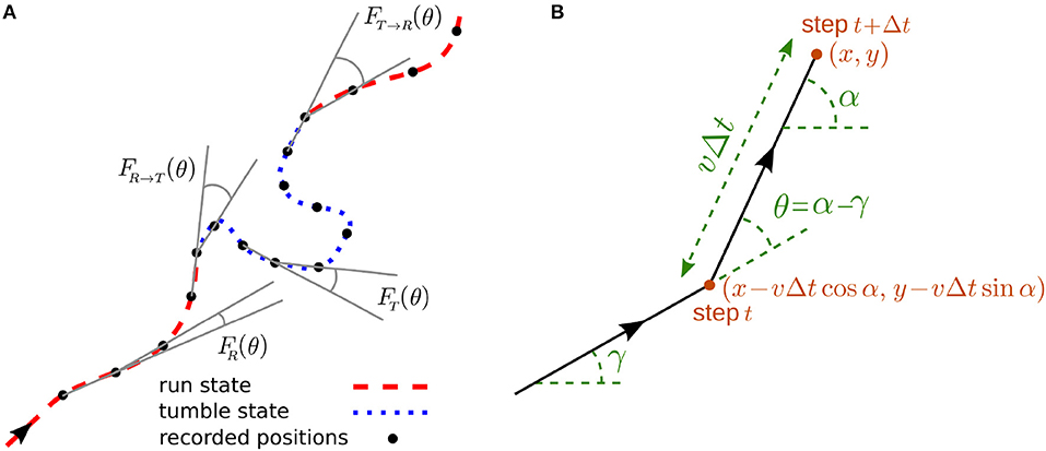
Figure 1. (A) A sample trajectory with run-and-tumble dynamics. Typical turning angles for different types of turning-angle distributions introduced in the model are shown. (B) Trajectory of the walker during two successive steps.

The run-and-tumble stochastic process can be described in discrete time by introducing the probability densities $P_t^R(x,y|\alpha )$ and $P_t^T(x,y|\alpha )$ to find the particle at position (x, y) arriving along the direction α at time t in the run and tumble states, respectively. α is defined with respect to a given reference direction, as shown in Figure 1B. Denoting the time interval between consecutive recorded positions of the particle by Δt, the following set of master equations describe the dynamical evolution of the probability densities

$\begin{array}{l}{P}_{{}_{t+\Delta t}}^R(x,y|\alpha )=\\ (1-f_{\text{R}\to \text{T}}){\displaystyle {\int }_{-\pi }^{\pi }d\gamma F_{\text{R}}(\alpha -\gamma )}{P}_t^R(x-v_{\text{R}}\Delta t\cos \alpha ,y-v_{\text{R}}\Delta t\sin \alpha |\gamma )\\ +f_{\text{T}\to \text{R}}{\displaystyle {\int }_{-\pi }^{\pi }d\gamma F_{\text{T}\to \text{R}}(\alpha -\gamma )P_t^T(x-v_{\text{R}}\Delta t\cos \alpha ,y-v_{\text{R}}\Delta t\sin \alpha |\gamma ),}\\ \\ P_{{}_{t+\Delta t}}^T(x,y|\alpha )=\\ (1-f_{\text{T}\to \text{R}}){\displaystyle {\int }_{-\pi }^{\pi }d\gamma F_{\text{T}}(\alpha -\gamma )}{P}_t^T(x-v_{\text{T}}\Delta t\cos \alpha ,y-v_{\text{T}}\Delta t\sin \alpha |\gamma )\\ +f_{\text{R}\to \text{T}}{\displaystyle {\int }_{-\pi }^{\pi }d\gamma F_{\text{R}\to \text{T}}{P}_t^R(x-v_{\text{T}}\Delta t\cos \alpha ,y-v_{\text{T}}\Delta t\sin \alpha |\gamma ).}& (1)\end{array}$

Each of the two terms on the right-hand side of the equations represents the possibility of being in one of the two states in the previous time step (see Figure 1B for the particle trajectory during two successive steps). The probability of starting the motion in the run or tumble phase is denoted by $P_0^R$ and $P_0^T$, respectively (with $P_0^T=1-P_0^R$). The change in the direction of motion θ = α−γ with respect to the arrival direction is randomly chosen according to the turning-angle distribution F_R(θ) or F_T(θ) in the run or tumble state, respectively. Both distributions are symmetric with respect to the arrival direction (i.e., left-right symmetric in 2D). We assume for simplicity that the directional change during the transition between the two states follows the turning-angle distribution of the new state, corresponding to F_{R → T}(θ) = F_T(θ) and F_{T → R}(θ) = F_R(θ). However, in general one should consider independent turning-angle distributions with non-zero mean for F_{R → T}(θ) and F_{T → R}(θ) as, for instance, a sharp change in the direction of motion of E. coli or Bacillus Subtilis when switching from tumbling to running is observed [1, 2, 6].

The total probability density P_t+Δt(x, y|α) to find the particle at position (x, y) arriving along the direction α at time t+Δt is given by $P_{t+\Delta t}(x,y|\alpha )=P_{t+\Delta t}^R(x,y|\alpha )+P_{t+\Delta t}^T(x,y|\alpha )$. Using the Fourier transform of the probability density in each state h (h∈{R, T}), defined as

$\begin{array}{ll}{P}_{{}_{t+\Delta t}}^h(k|m)\equiv {\displaystyle {\int }_{-\pi }^{\pi }}\text{ d}\alpha e^{im\alpha }{\displaystyle \int }\text{ d}y{\displaystyle \int }\text{ d}x{e}^{ik·r}{P}_{{}_{t+\Delta t}}^h(x,y|\alpha ),& (2)\end{array}$

the Fourier transform of the total probability density is given by $P_{t+\Delta t}(k|m)=P_{t+\Delta t}^R(k|m)+P_{t+\Delta t}^T(k|m)$, from which the moments of displacement can be calculated as

$\begin{array}{l}\langle x^{j_1}{y}^{j_2}\rangle (t+\Delta t)\equiv {\displaystyle \int }\text{ d}\alpha {\displaystyle \int }\text{ d}y{\displaystyle \int }\text{ d}x{x}^{j_1}{y}^{j_2}{P}_{{}_{t+\Delta t}}(x,y|\alpha )\\ ={\left(-i\right)}^{j1+j2}\frac{{\partial }^{j_1+j_2}{P}_{{}_{t+\Delta t}}(k_x,k_y|m=0)}{\partial k_x^{j_1}\partial k_y^{j_2}}{|}_{(k_x,k_y)=(0,0)}.& (3)\end{array}$

By means of a Fourier-z-transform technique, it is possible to solve the master equations (1) to obtain the time evolution of the moments of displacement [38–40]. Here we briefly explain the procedure to calculate the mean square displacement (MSD) as the main quantity of interest. From Equation (3), the MSD is given as

$\begin{array}{ll}\langle r^2\rangle \left(t+\Delta t\right)={\left(-i\right)}^2\frac{{\partial }^2{P}_{{}_{t+\Delta t}}(k,\varphi =0|m=0)}{\partial k^2}{|}_{k=0},& (4)\end{array}$

where (k, ϕ) is the polar representation of k. Assuming $F_{\text{R}\to \text{T}}(\theta )=F_{\text{T}}(\theta )=\frac{1}{2\pi }$ and F_{T → R}(θ) = F_R(θ), their Fourier transforms are $F_{\text{R}\to \text{T}}(m)=F_{\text{T}}(m)=\frac{1}{2\pi }{\int }_{-\pi }^{\pi }\text{d}\theta e^{im\theta }$ and $F_{\text{T}\to \text{R}}(\theta )=F_{\text{R}}(m)={\int }_{-\pi }^{\pi }\text{d}\theta e^{im\theta }{F}_{\text{R}}(\theta )$. Next we apply the Fourier transformation on the master equations (1). For example, the first master equation after Fourier transform reads

$\begin{array}{l}{P}_{{}_{t+\Delta t}}^R(k,\varphi |m)=\\ (1-f_{\text{R}\to \text{T}}){\displaystyle \int }\text{ d}\alpha e^{im\alpha }{\displaystyle \int }d\gamma F_{\text{R}}(\alpha -\gamma ){\displaystyle \int }\text{ d}y{\displaystyle \int }\text{ d}x{e}^{ik·r}\\ P_t^R(x-v_{\text{R}}\Delta t\cos \alpha ,y-v_{\text{R}}\Delta t\sin \alpha |\gamma )\\ +f_{\text{T}\to \text{R}}{\displaystyle \int }\text{ d}\alpha e^{im\alpha }{\displaystyle \int }d\gamma F_{\text{T}\to \text{R}}(\alpha -\gamma ){\displaystyle \int }\text{ d}y{\displaystyle \int }\text{ d}x{e}^{ik·r}{P}_t^T\\ (x-v_{\text{R}}\Delta t\cos \alpha ,y-v_{\text{R}}\Delta t\sin \alpha |\gamma ).& (5)\end{array}$

Then by using the qth order Bessel's function

$\begin{array}{l}{J}_q(z)=\frac{1}{2\pi i^q}{\displaystyle {\int }_{-\pi }^{\pi }\text{d}\alpha e^{iz\cos \alpha }{e}^{-iq\alpha }},\end{array}$

replacing $e^{ik{v}_{\text{R}}\Delta t\cos \left(\alpha -\varphi \right)}$ with ${\int }_{-\pi }^{\pi }d\beta e^{ik{v}_{\text{R}}\Delta t\cos \beta }\delta \left(\beta -\left(\alpha -\varphi \right)\right)$, and using

$\begin{array}{l}\delta (\beta -(\alpha -\varphi ))=\frac{1}{2\pi }{\displaystyle \sum _{q=-\infty }^{\infty }{e}^{-iq(\beta -(\alpha -\varphi ))}},\end{array}$

it follows that

$\begin{array}{l}{P}_{{}_{t+\Delta t}}^{\text{R}}(k,\varphi |m)={\displaystyle \sum _{q=-\infty }^{\infty }}{i}^q{e}^{-iq\varphi }{J}_q(k{v}_{\text{R}}\Delta t)\times \\ [(1-f_{\text{R}\to \text{T}})F_{\text{R}}(m+q)P_t^{\text{R}}(k,\varphi |m+q)\\ +f_{\text{T}\to \text{R}}{F}_{\text{R}}(m+q)P_t^{\text{T}}(k,\varphi |m+q)].& (6)\end{array}$

$P_{t+\Delta t}^R(k,\varphi |m)$ can be expanded as a Taylor series

$\begin{array}{l}{P}_{t+\Delta t}^R(k,\varphi |m)=Q_{0,t+\Delta t}^R(\varphi |m)+ik{v}_{\text{R}}\Delta t{Q}_{1,t+\Delta t}^R(\varphi |m)\\ -\frac{1}{2}{k}^2{v}_{\text{R}}^2{\left(\Delta t\right)}^2{Q}_{2,t+\Delta t}^R(\varphi |m)+···.& (7)\end{array}$

We expand both sides of Equation (6) and collect all terms with the same power in k. As a result, recursion relations for the Taylor expansion coefficients can be obtained. For instance, for the terms with power 0 in k one finds

$\begin{array}{l}{Q}_{0,t+\Delta t}^{\text{R}}(\varphi |m)=(1-f_{\text{R}\to \text{T}})F_{\text{R}}(m)Q_{0,t}^{\text{R}}(\varphi |m)\\ +f_{\text{T}\to \text{R}}{F}_{\text{R}}(m)Q_{0,t}^{\text{T}}(\varphi |m).& (8)\end{array}$

Similarly, the expansion coefficients of terms with higher powers in k can be calculated and the procedure is repeated for the second master equation in (1). As a result, a set of coupled equations is obtained for each expansion coefficient, connecting time steps t+Δt and t. Applying a z-transform $Q(z)={\sum }_{t=0}^{\infty }{Q}_t{z}^{-t}$ enables one to solve these sets of equations. Particularly the coefficients of terms with power 2 in k, i.e., $Q_2^{\text{R}}(z,\varphi |m)$ and $Q_2^{\text{T}}(z,\varphi |m)$, are useful to calculate the MSD

$\begin{array}{ll}\langle r^2\rangle (z)=2{(\Delta t)}^2(v_{\text{R}}^2{Q}_2^{\text{R}}(z,0|0)+v_{\text{T}}^2{Q}_2^{\text{T}}(z,0|0)).& (9)\end{array}$

Finally we obtain the following exact expression for the MSD in z space

$\begin{array}{l}\langle r^2\rangle (z)=[\frac{z(1-f_{\text{R}\to \text{T}}-f_{\text{T}\to \text{R}})P_0^R}{z-1+f_{\text{R}\to \text{T}}+f_{\text{T}\to \text{R}}}+\frac{z^2{f}_{\text{T}\to \text{R}}}{G_0(z)}][\frac{2z^2}{(z-1)G_1(z)}-\frac{1}{(z-1}]v_{\text{R}}^2{(\Delta t)}^2\hfill \\ +[\frac{-z(1-f_{\text{R}\to \text{T}}-f_{\text{T}\to \text{R}})P_0^R}{z-1+f_{\text{R}\to \text{T}}+f_{\text{T}\to \text{R}}}+\frac{z^2(1-f_{\text{T}\to \text{R}})}{G_0(z)}-\frac{z(1-f_{\text{T}\to \text{R}}-f_{\text{R}\to \text{T}})}{G_0(z)}]\hfill \\ \times [\frac{2z[z-(1-f_{\text{R}\to \text{T}})p]}{(z-1)G_1(z)}{v}_{\text{T}}^2+\frac{2z}{(z-1)G_1(z)}{f}_{\text{T}\to \text{R}}p{v}_{\text{R}}{v}_{\text{T}}-\frac{1}{z-1}{v}_{\text{T}}^2]{(\Delta t)}^2,\hfill & (10)\end{array}$

where G₀(z)=(z−1)(z−1+f_{T → R}+f_{R → T}) and $G_1\left(z\right)=z\left(z-\left(1-f_{\text{R}\to \text{T}}\right)p\right)$. By inverse z-transforming Equation (10), the MSD can be obtained as a function of time. The resulting general expression for the MSD 〈r²〉(t) is lengthy and depends on the run persistency p, the speeds v_R and v_T, the transition probabilities f_{R → T} and f_{T → R}, and the probability of initially starting in the run $P_0^R$ or tumble state $P_0^T=1-P_0^R$. 〈r²〉(t) typically consists of linear and exponentially decaying terms with t as well as time-independent terms, as shown in the following in the special case of constant velocity and the initial condition of starting in the run state. By choosing Δt = 1, v_R = v_T = 1, and the initial condition $P_0^R=1$, the general expression of 〈r²〉(t) reduces to.

$\begin{array}{l}\langle r^2\rangle (t)=\frac{(p((f_{\text{T}\to \text{R}}-1)f_{\text{R}\to \text{T}}+f_{\text{T}\to \text{R}}+f_{\text{R}\to \text{T}}^2)+f_{\text{T}\to \text{R}}+f_{\text{R}\to \text{T}})}{p(f_{\text{R}\to \text{T}}-1)(f_{\text{T}\to \text{R}}+f_{\text{R}\to \text{T}})+f_{\text{T}\to \text{R}}+f_{\text{R}\to \text{T}}}t-\\ \frac{2p(f_{\text{R}\to \text{T}}-1)(f_{\text{R}\to \text{T}}p(f_{\text{T}\to \text{R}}+f_{\text{R}\to \text{T}}-2)+f_{\text{T}\to \text{R}}+f_{\text{R}\to \text{T}}+p-1)(p(1-f_{\text{R}\to \text{T}}){)}^t}{(p(f_{\text{R}\to \text{T}}-1)+1{)}^2(f_{\text{T}\to \text{R}}-f_{\text{R}\to \text{T}}p+f_{\text{R}\to \text{T}}+p-1)}\\ +\frac{2p{f}_{\text{R}\to \text{T}}{(1-f_{\text{T}\to \text{R}}-f_{\text{R}\to \text{T}})}^{t+2}}{{(f_{\text{T}\to \text{R}}+f_{\text{R}\to \text{T}})}^2(f_{\text{T}\to \text{R}}-f_{\text{R}\to \text{T}}p+f_{\text{R}\to \text{T}}+p-1)}+\\ \frac{(p((f_{\text{T}\to \text{R}}-1)f_{\text{R}\to \text{T}}+f_{\text{T}\to \text{R}}+f_{\text{R}\to \text{T}}^2)+f_{\text{T}\to \text{R}}+f_{\text{R}\to \text{T}})}{p(f_{\text{R}\to \text{T}}-1)(f_{\text{T}\to \text{R}}+f_{\text{R}\to \text{T}})+f_{\text{T}\to \text{R}}+f_{\text{R}\to \text{T}}}-\\ \frac{2p({(f_{\text{T}\to \text{R}}+f_{\text{R}\to \text{T}})}^2-f_{\text{R}\to \text{T}})+{(f_{\text{T}\to \text{R}}+f_{\text{R}\to \text{T}})}^2}{(p(f_{\text{R}\to \text{T}}-1)(f_{\text{T}\to \text{R}}+f_{\text{R}\to \text{T}})+f_{\text{T}\to \text{R}}+f_{\text{R}\to \text{T}}{)}^2}+\\ \frac{p^2(f_{\text{R}\to \text{T}}-1)((f_{\text{T}\to \text{R}}+f_{\text{R}\to \text{T}})(f_{\text{T}\to \text{R}}(f_{\text{R}\to \text{T}}-1)+(f_{\text{R}\to \text{T}}-3)f_{\text{R}\to \text{T}})+2f_{\text{R}\to \text{T}})}{(p(f_{\text{R}\to \text{T}}-1)(f_{\text{T}\to \text{R}}+f_{\text{R}\to \text{T}})+f_{\text{T}\to \text{R}}+f_{\text{R}\to \text{T}}{)}^2}.& (11)\end{array}$

3. Results and Discussion

We first investigate the time evolution of the MSD for different values of the key parameters p, v_R, v_T, f_{R → T}, f_{T → R}, and $P_0^R$. As a simple check, the expression (10) for f_{R → T} = 0, f_{T → R} = 1, v_T = 0, and $P_0^R=1$ reduces to

$\begin{array}{ll}\langle r^2\rangle (z)=\frac{v_{\text{R}}^{2}z(z+p)}{{(z-1)}^2(z-p)}{(\Delta t)}^2,& (12)\end{array}$

and by inverse z-transforming, the MSD for a single-state persistent random walk [37, 41]

$\begin{array}{ll}\langle r^2\rangle (t)={\left(\Delta t\right)}^2{v}_{\text{R}}^2\left[\frac{1+p}{1-p}t+2p\frac{p^t-1}{{(1-p)}^2}\right]& (13)\end{array}$

is recovered. In Figure 2, we show how the MSD evolves in time for different values of the key parameters. We plot the general expression of 〈r²〉(t), obtained from the inverse z-transforming of Equation (10), and validate the analytical predictions by Monte Carlo simulations. A wide range of different types of anomalous dynamics can be observed on varying the parameters. While the short-time dynamics is typically superdiffusion (due to the combination of active and passive motion) and the long-term dynamics is diffusion in all cases, transitions between sub-, ordinary, and super-diffusion occur on short and intermediate time scales. For some parameter values, the exponential terms of the MSD rapidly decay while the linear term is not yet big enough compared to the time-independent terms. In such a case, the constant terms dominate at intermediate time scales leading to the observed slow dynamics in this regime. The asymptotic dynamics is however diffusive since the linear term eventually dominates. It can also be seen that the crossover time to asymptotic diffusion varies by several orders of magnitude upon changing the parameter values. The crossover time can be characterized as the time at which the exponentially decreasing terms in 〈r²〉(t) become smaller than the terms which survive at long times. We find that the convergence of the MSD to its asymptotic diffusive form can be described by the sum of two exponential functions

$\begin{array}{ll}\langle r^2\rangle (t)-\langle r^2\rangle (t\to \infty )~B_1{\text{e}}^{-t/t_{c_1}}+B_2{\text{e}}^{-t/t_{c_2}},& (14)\end{array}$

with the characteristic times $t_{c_1}=\frac{1}{|ln(1-f_{\text{R}\to \text{T}}-f_{\text{T}\to \text{R}})|}$ and $t_{c_2}=\frac{1}{|ln(p(1-f_{\text{R}\to \text{T}}))|}$. The prefactors B₁ and B₂ are functions of p, v_R, v_T, f_{R → T}, f_{T → R}, and $P_0^R$. Figure 3 shows how the characteristic times t_c1 and t_c2 vary upon changing the key parameters. Although the slopes of the exponential decays in Equation (14) are solely determined by the transition probabilities f_{R → T} and f_{T → R} and the run persistency p, the crossover time to the asymptotic diffusive dynamics is also influenced by the other dynamic parameters of the model through the prefactors B₁ and B₂. For example, for the set of parameter values p = 0.9, v_R = 10, v_T = 0.1, f_{R → T} = 0.1, and f_{T → R} = 0.01, the convergence time (with 5% accuracy) to the asymptotic dynamics for $P_0^R=1$ is nearly twice as long as for $P_0^R=0$.

FIGURE 2

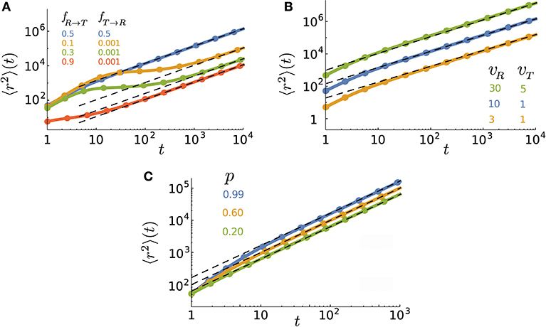
Figure 2. Time evolution of the MSD for various (A) transition probabilities, (B) speeds, and (C) persistencies. The parameter values (unless varied) are taken to be p = 0.9, v_R = 10, v_T = 1, Δt = 1, f_{R → T} = 0.5, f_{T → R} = 0.5, and $P_0^R=0.5$. The lines are obtained from the inverse z-transform of Equation (10) and symbols denote simulation results. The dashed lines represent the asymptotic diffusion regime.

FIGURE 3

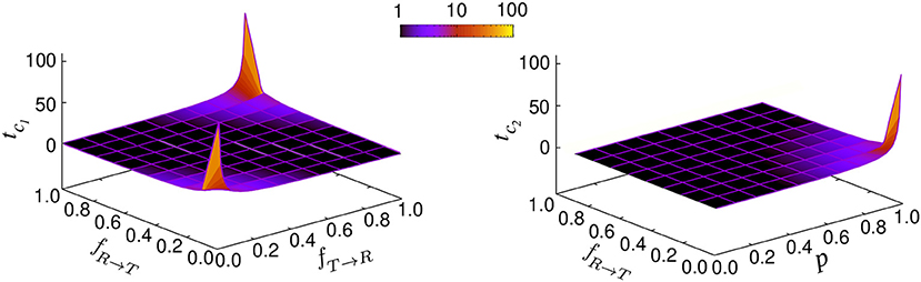
Figure 3. Characteristic times t_c1 and t_c2 in terms of the transition probabilities f_{R → T} and f_{T → R} and run persistency p.

Figure 2 also shows that the asymptotic diffusion constant D_asymp varies by changing the key parameters. The differences in the y-intercept of the dashed (asymptotic) lines in log-log plots reflect the sensitivity of D_asymp to the model parameters. By inverse z-transforming of Equation (10) and taking the limit t → ∞, we obtain D_asymp (i.e., the coefficient of the term linear in time) in the general form as

$\begin{array}{l}{D}_{\text{asymp}}=\\ \frac{1}{4}\Delta t\frac{2f_{\text{T}\to \text{R}}{f}_{\text{R}\to \text{T}}p{v}_{\text{T}}{v}_{\text{R}}+f_{\text{T}\to \text{R}}{v}_{\text{R}}^2(1+p(1-f_{\text{R}\to \text{T}}))+f_{\text{R}\to \text{T}}{v}_{\text{T}}^2(1-p(1-f_{\text{R}\to \text{T}}))}{(f_{\text{T}\to \text{R}}+f_{\text{R}\to \text{T}})(1-p(1-f_{\text{R}\to \text{T}}))}& (15)\end{array}$

While the diffusion coefficient trivially increases with the speed, its dependency on f_{R → T}, f_{T → R}, and p is more complicated and shown in Figure 4. D_asymp varies by several orders of magnitude as a function of these parameters. Under the specific condition F_{R → T}(θ) = F_T(θ) = δ(θ) and F_{T → R}(θ) = F_R(θ) and v_T = 0, the walker stops when entering the tumble phase without changing its arrival direction and it returns smoothly to the run phase without experiencing a kick (i.e., a sharp change in the direction of motion). Motor-driven transport along cytoskeletal filaments in crowded cytoplasm exhibits such a run-and-pause dynamics [21, 42]. In this case, one obtains

$\begin{array}{ll}{D}_{\text{asymp}}^{\text{run-pause}}=\frac{1}{4}\Delta t{v}_{\text{R}}^2\frac{1+p}{1-p}\frac{f_{\text{T}\to \text{R}}}{f_{\text{T}\to \text{R}}+f_{\text{R}\to \text{T}}}& (16)\end{array}$

In the limit p → 1 the trajectory becomes nearly straight implying that the randomization time and the covered area until reaching the asymptotic diffusive regime (and thus D_asymp) diverge.

FIGURE 4

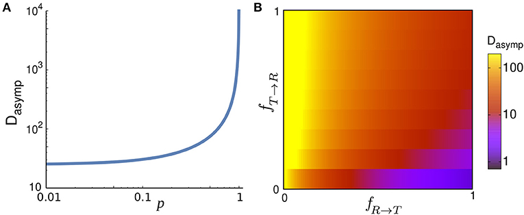
Figure 4. (A) Asymptotic diffusion coefficient D_asymp as a function of the run persistency p for v_R = 10, v_T = 1, Δt = 1, f_{R → T} = 0.001, and f_{T → R} = 0.9. (B) D_asymp in the space of transition probabilities f_{R → T} and f_{T → R} for v_R = 10, v_T = 1, Δt = 1, and p = 0.9.

Interestingly, D_asymp in Equation (15) is independent of $P_0^R$ and $P_0^T$, i.e., the initial condition of starting the motion in the run or tumble state. Thus, the analytical results predict that the asymptotic diffusive dynamics, characterized by the linear time-dependence

$\begin{array}{ll}\langle r^2\rangle (t\to \infty )=4D_{\text{asymp}}t,& (17)\end{array}$

does not depend on the initial conditions. In Figure 5 we present the simulation results for several values of $P_0^R$. At long times, all curves merge and follow the analytical prediction Equation (17). Note that only the linear term in time is independent of $P_0^R$ and the exponentially decaying and time-independent terms in the MSD depend on the initial conditions (see e.g., Equation 12). The walker keeps initially for some time its memory of the initial direction and state of motion. However, the influence of the $P_0^R$-dependent terms vanishes in the limit t → ∞ and the time dependence of the MSD approaches the asymptotic linear form Equation (17).

FIGURE 5

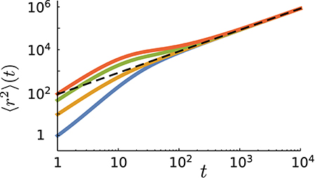
Figure 5. The mean square displacement as a function of time for different values of the probability $P_0^R$ of initially starting in the run state in simulations (from top to bottom: $P_0^R=1.0,0.5,0.1,0.0$). Other parameter values: p = 0.9, v_R = 10, v_T = 0.1, f_{R → T} = 0.1, and f_{T → R} = 0.01. The dashed line represents the analytical prediction via Equation (17) for the same parameter values.

The short time dynamics is, however, strongly influenced by the choice of the initial conditions. Figure 5 shows that the initial slope of the MSD curve varies with $P_0^R$. One can assign an initial anomalous exponent κ to the MSD curve by fitting the power-law 〈r²〉~t^κ. By choosing the first two data points of the MSD curve, the fitting leads to 〈r²〉(t = 2)/〈r²〉(t = 1) = 2^κ. Thus, the initial anomalous exponent κ can be deduced from the MSD at t = 1, 2 as

$\begin{array}{ll}\kappa =\ln \left[\frac{\langle r^2\rangle (t=2)}{\langle r^2\rangle (t=1)}\right]/\ln 2,& (18)\end{array}$

After replacing the MSD at t = 1, 2 obtained from Equation (10) we get

$\begin{array}{l}\kappa =\ln \left[[(2-2P_0^R+(3-f_{\text{T}\to \text{R}}-f_{\text{R}\to \text{T}})(f_{\text{T}\to \text{R}}(P_0^R-1+f_{\text{R}\to \text{T}}{P}_0^R)\right)v_{\text{T}}^2\\ +2f_{\text{T}\to \text{R}}(1-f_{\text{T}\to \text{R}}+(f_{\text{T}\to \text{R}}+f_{\text{R}\to \text{T}}-1)P_0^R)p{v}_{\text{T}}{v}_{\text{R}}\\ +(2P_0^R+(-3+f_{\text{T}\to \text{R}}+f_{\text{R}\to \text{T}})(f_{\text{T}\to \text{R}}+(P_0^R-1)+f_{\text{R}\to \text{T}}{P}_0^R)\\ +2(f_{\text{R}\to \text{T}}-1)(-f_{\text{T}\to \text{R}}+(f_{\text{T}\to \text{R}}+f_{\text{R}\to \text{T}}-1)P_0^R)p)v_R^2]/\\ \left[(1-f_{\text{T}\to \text{R}}-(1-f_{\text{T}\to \text{R}}-f_{\text{R}\to \text{T}})P_0^R)v_{\text{T}}^2+(f_{\text{T}\to \text{R}}-(1-f_{\text{T}\to \text{R}}-f_{\text{R}\to \text{T}})P_0^R)v_R^2\right]]\text{In }2.& (19)\end{array}$

Figure 6A shows the influence of the initial conditions on the initial anomalous exponent for a given set of parameters. Note that the monotonic growth of κ with $P_0^R$ does not hold in general, as we observed decreasing as well as non-monotonic dependencies by varying other parameter values. However, κ increases monotonically with p in all parameter regimes as shown in Figure 6B. Moreover, Figures 6C,D show that κ also varies widely with the speed and transition probabilities. Because of combining an active run state (0<p<1) and normal diffusion (tumble state), κ remains above 1 (superdiffusion). However, by generalizing the run state to include subdiffusive motion (i.e., when −1<p<1), κ can decrease below 1.

FIGURE 6

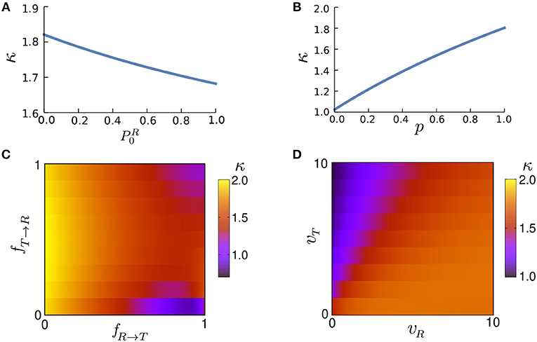
Figure 6. The anomalous exponent κ vs. (A) the initial condition of motion $P_0^R$, (B) run persistency p, (C) transition probabilities f_{R → T} and f_{T → R}, and (D) speeds v_R and v_T via Equation (19). The parameter values (unless varied) are taken to be p = 0.9, v_R = 10, v_T = 1, Δt = 1, f_{R → T} = 0.3, f_{T → R} = 0.5, and $P_0^R=0.5$.

To better understand the role of the initial conditions, we note that the steady probabilities $P_{\text{steady}}^R$ and $P_{\text{steady}}^T$ of finding the particle in each of the two states are determined by the transition probabilities f_{R → T} and f_{T → R}. Therefore, the influence of the initial condition of starting the motion in any of the two states gradually vanishes as the probabilities P^R(t) and P^T(t) of finding the particle in the run or tumble state gradually approach their steady values. By considering a discrete time Markov process with transition probabilities f_{R → T} and f_{T → R}, the probabilities at time t can be obtained from those at time t−1 as

$\begin{array}{ll}(P^R(t),P^T(t))=(P^R(t-1),P^T(t-1))\left[\begin{array}{ll}1-f_{\text{R}\to \text{T}}\hfill & f_{\text{R}\to \text{T}}\hfill \\ f_{\text{T}\to \text{R}}\hfill & 1-f_{\text{T}\to \text{R}}\hfill \end{array}\right].& (20)\end{array}$

By applying this relation recursively, one can derive the probabilities at time t based on the initial probabilities

$\begin{array}{l}(P^R(t),P^T(t))=(P_0^R,P_0^T){\left[\begin{array}{ll}1-f_{\text{R}\to \text{T}}\hfill & f_{\text{R}\to \text{T}}\hfill \\ f_{\text{T}\to \text{R}}\hfill & 1-f_{\text{T}\to \text{R}}\hfill \end{array}\right]}^t\\ =(P_0^R,P_0^T)\frac{1}{f_{\text{R}\to \text{T}}+f_{\text{R}\to \text{T}}}\\ \left[\begin{array}{ll}{f}_{\text{T}\to \text{R}}+f_{\text{R}\to \text{T}}{(1-f_{\text{T}\to \text{R}}-f_{\text{R}\to \text{T}})}^t\hfill & f_{\text{R}\to \text{T}}\left(1-{(1-f_{\text{T}\to \text{R}}-f_{\text{R}\to \text{T}})}^t\right)\hfill \\ f_{\text{T}\to \text{R}}\left(1-{(1-f_{\text{T}\to \text{R}}-f_{\text{R}\to \text{T}})}^t\right)\hfill & f_{\text{R}\to \text{T}}+f_{\text{T}\to \text{R}}{(1-f_{\text{T}\to \text{R}}-f_{\text{R}\to \text{T}})}^t\hfill \end{array}\right].& (21)\end{array}$

Thus the evolution of P^R(t) and P^T(t) obeys

$\begin{array}{l}{P}^R(t)=\frac{f_{\text{T}\to \text{R}}}{f_{\text{T}\to \text{R}}+f_{\text{R}\to \text{T}}}+\frac{{\left(1-f_{\text{T}\to \text{R}}-f_{\text{R}\to \text{T}}\right)}^t}{f_{\text{T}\to \text{R}}+f_{\text{R}\to \text{T}}}\\ \left(f_{\text{R}\to \text{T}}{P}_0^R-f_{\text{T}\to \text{R}}(1-P_0^R)\right),\\ P^T(t)=\frac{f_{\text{R}\to \text{T}}}{f_{\text{T}\to \text{R}}+f_{\text{R}\to \text{T}}}-\frac{{\left(1-f_{\text{T}\to \text{R}}-f_{\text{R}\to \text{T}}\right)}^t}{f_{\text{T}\to \text{R}}+f_{\text{R}\to \text{T}}}\\ \left(f_{\text{R}\to \text{T}}{P}_0^R-f_{\text{T}\to \text{R}}(1-P_0^R)\right),& (22)\end{array}$

leading to the steady probabilities $P_{\text{steady}}^R=\frac{f_{\text{T}\to \text{R}}}{f_{\text{T}\to \text{R}}+f_{\text{R}\to \text{T}}}$ and $P_{\text{steady}}^T=\frac{f_{\text{R}\to \text{T}}}{f_{\text{T}\to \text{R}}+f_{\text{R}\to \text{T}}}$. If one starts with the initial condition $P_0^R=P_{\text{steady}}^R$, the system is immediately equilibrated. Otherwise, the choice of the initial conditions affects the short-time dynamics and diversifies the transient anomalous diffusive regimes. According to Equation (21), the relaxation of the probabilities toward their steady values follow an exponential decay $P^R(t),P^T(t)~{\text{e}}^{-t/t_m}$ with $t_m=\frac{1}{|ln(1-f_{\text{R}\to \text{T}}-f_{\text{T}\to \text{R}})|}$. While the characteristic relaxation time of the probabilities solely depends on the transition probabilities, the characteristic time for the crossover to asymptotic dynamics is influenced additionally by the run persistency, as we showed previously in Equation (14).

Therefore, there are two independent relaxation times t_m(= t_c1) and t_c2. In case these differ substantially, two distinct crossovers in the time evolution of the MSD may be observed in general as can be seen in Figure 2A.

4. Conclusion

We presented a persistent random walk model to study the stochastic dynamics of particles with active fast and passive slow motility modes. We derived an exact analytical expression for the mean square displacement, which allows to analyze the transient anomalous transport regimes on short time scales and also to extract the characteristics of the asymptotic diffusive motion such as the crossover time and the long-term diffusion constant. In particular we showed that while the choice of the initial conditions influences the anomalous diffusion at short times, the asymptotic behavior remains independent of it and is entirely controlled by the run persistency, the velocities of the run and tumble states and the transition probabilities between the two states.

Data Availability

All datasets generated for this study are included in the manuscript and the Supplementary Files.

Author Contributions

MS and HR designed the study, performed the analysis, and wrote the manuscript.

Funding

This work was financially supported by the German Research Foundation (DFG) within the Collaborative Research Center SFB 1027 (A3, A7).

Conflict of Interest Statement

The authors declare that the research was conducted in the absence of any commercial or financial relationships that could be construed as a potential conflict of interest.

References

1. Berg HC. E. coli in Motion. New York, NY: Springer Verlag (2004).

Google Scholar

2. Berg HC, Brown DA. Chemotaxis in Escherichia coli analysed by three-dimensional tracking. Nature. (1972) 239:500–4. doi: 10.1038/239500a0

PubMed Abstract | CrossRef Full Text | Google Scholar

3. Patteson AE, Gopinath A, Goulian M, Arratia PE. Running and tumbling with E. coli in polymeric solutions. Sci Rep. (2015) 5:15761. doi: 10.1038/srep15761

PubMed Abstract | CrossRef Full Text | Google Scholar

4. Bartumeus F, Levin SA. Fractal reorientation clocks: linking animal behavior to statistical patterns of search. Proc Natl Acad Sci USA. (2008) 105:19072–7. doi: 10.1073/pnas.0801926105

PubMed Abstract | CrossRef Full Text | Google Scholar

5. Bénichou O, Coppey M, Moreau M, Suet PH, Voituriez R. Optimal search strategies for hidden targets. Phys Rev Lett. (2005) 94:198101. doi: 10.1103/PhysRevLett.94.198101

PubMed Abstract | CrossRef Full Text | Google Scholar

6. Najafi J, Shaebani MR, John T, Altegoer F, Bange G, Wagner C. Flagellar number governs bacterial spreading and transport efficiency. Sci Adv. (2018) 4:eaar6425. doi: 10.1126/sciadv.aar6425

PubMed Abstract | CrossRef Full Text | Google Scholar

7. Bénichou O, Loverdo C, Moreau M, Voituriez R. Intermittent search strategies. Rev Mod Phys. (2011) 83:81–129. doi: 10.1103/RevModPhys.83.81

CrossRef Full Text | Google Scholar

8. Wadhams GH, Armitage JP. Making sense of it all: bacterial chemotaxis. Nat Rev Mol Cell Biol. (2004) 5:1024–37. doi: 10.1038/nrm1524

PubMed Abstract | CrossRef Full Text | Google Scholar

9. Taktikos J, Stark H, Zaburdaev V. How the motility pattern of bacteria affects their dispersal and chemotaxis. PLoS ONE. (2014) 8:e81936. doi: 10.1371/journal.pone.0081936

PubMed Abstract | CrossRef Full Text | Google Scholar

10. Weigel AV, Simon B, Tamkun MM, Krapf D. Ergodic and nonergodic processes coexist in the plasma membrane as observed by single-molecule tracking. Proc Natl Acad Sci USA. (2011) 108:6438–43. doi: 10.1073/pnas.1016325108

PubMed Abstract | CrossRef Full Text | Google Scholar

11. Guigas G, Weiss M. Sampling the ell with anomalous diffusion-the discovery of slowness. Biophys J. (2008) 94:90–4. doi: 10.1529/biophysj.107.117044

CrossRef Full Text | Google Scholar

12. Golding I, Cox EC. Physical nature of bacterial cytoplasm. Phys Rev Lett. (2006) 96:098102. doi: 10.1103/PhysRevLett.96.098102

PubMed Abstract | CrossRef Full Text | Google Scholar

13. Sereshki LE, Lomholt MA, Metzler R. A solution to the subdiffusion-efficiency paradox: Inactive states enhance reaction efficiency at subdiffusion conditions in living cells. EPL. (2012) 97:20008. doi: 10.1209/0295-5075/97/20008

CrossRef Full Text | Google Scholar

14. Ali MY, Krementsova EB, Kennedy GG, Mahaffy R, Pollard TD, Trybus KM, et al. Myosin Va maneuvers through actin intersections and diffuses along microtubules. Proc Natl Acad Sci USA. (2007) 104:4332–6. doi: 10.1073/pnas.0611471104

PubMed Abstract | CrossRef Full Text | Google Scholar

15. Shiroguchi K, Kinosita K. Myosin V walks by lever action and brownian motion. Science. (2007) 316:1208–12. doi: 10.1126/science.1140468

PubMed Abstract | CrossRef Full Text | Google Scholar

16. Vershinin M, Carter BC, Razafsky DS, King SJ, Gross SP. Multiple-motor based transport and its regulation by Tau. Proc Natl Acad Sci USA. (2007) 104:87–92. doi: 10.1073/pnas.0607919104

PubMed Abstract | CrossRef Full Text | Google Scholar

17. Okada Y, Higuchi H, Hirokawa N. Processivity of the single-headed kinesin KIF1A through biased binding to tubulin. Nature. (2003) 424:574–7. doi: 10.1038/nature01804

PubMed Abstract | CrossRef Full Text | Google Scholar

18. Culver-Hanlon TL, Lex SA, Stephens AD, Quintyne NJ, King SJ. A microtubule-binding domain in dynactin increases dynein processivity by skating along microtubules. Nat Cell Biol. (2006) 8:264–70. doi: 10.1038/ncb1370

PubMed Abstract | CrossRef Full Text | Google Scholar

19. Klumpp S, Lipowsky R. Active diffusion of motor particles. Phys Rev Lett. (2005) 95:268102. doi: 10.1103/PhysRevLett.95.268102

PubMed Abstract | CrossRef Full Text | Google Scholar

20. Lipowsky R, Klumpp S. Life is motion: multiscale motility of molecular motors. Physica A. (2005) 352:53–112. doi: 10.1016/j.physa.2004.12.034

CrossRef Full Text | Google Scholar

21. Hafner AE, Santen L, Rieger H, Shaebani MR. Run-and-pause dynamics of cytoskeletal motor proteins. Sci Rep. (2016) 6:37162. doi: 10.1038/srep37162

PubMed Abstract | CrossRef Full Text | Google Scholar

22. Pinkoviezky I, Gov NS. Transport dynamics of molecular motors that switch between an active and inactive state. Phys Rev E. (2013) 88:022714. doi: 10.1103/PhysRevE.88.022714

PubMed Abstract | CrossRef Full Text | Google Scholar

23. Chabaud M, Heuzé ML, Bretou M, Vargas P, Maiuri P, Solanes P, et al. Cell migration and antigen capture are antagonistic processes coupled by myosin II in dendritic cells. Nat Commun. (2015) 6:7526. doi: 10.1038/ncomms8526

CrossRef Full Text | Google Scholar

24. Bressloff PC, Newby JM. Stochastic models of intracellular transport. Rev Mod Phys. (2013) 85:135–96. doi: 10.1103/RevModPhys.85.135

CrossRef Full Text | Google Scholar

25. Höfling F, Franosch T. Anomalous transport in the crowded world of biological cells. Rep Prog Phys. (2013) 76:046602. doi: 10.1088/0034-4885/76/4/046602

PubMed Abstract | CrossRef Full Text | Google Scholar

26. Jose R, Santen L, Shaebani MR. Trapping in and escape from branched structures of neuronal dendrites. Biophys J. (2018) 115:2014–25. doi: 10.1016/j.bpj.2018.09.029

PubMed Abstract | CrossRef Full Text | Google Scholar

27. Angelani L. Averaged run-and-tumble walks. EPL. (2013) 102:20004. doi: 10.1209/0295-5075/102/20004

CrossRef Full Text | Google Scholar

28. Soto R, Golestanian R. Run-and-tumble dynamics in a crowded environment: persistent exclusion process for swimmers. Phys Rev E. (2014) 89:012706. doi: 10.1103/PhysRevE.89.012706

PubMed Abstract | CrossRef Full Text | Google Scholar

29. Shaebani MR, Pasula A, Ott A, Santen L. Tracking of plus-ends reveals microtubule functional diversity in different cell types. Sci Rep. (2016) 6:30285. doi: 10.1038/srep30285

PubMed Abstract | CrossRef Full Text | Google Scholar

30. Theves M, Taktikos J, Zaburdaev V, Stark H, Beta C. A bacterial swimmer with two alternating speeds of propagation. Biophys J. (2013) 105:1915–24. doi: 10.1016/j.bpj.2013.08.047

PubMed Abstract | CrossRef Full Text | Google Scholar

31. Shaebani MR, Jose R, Sand C, Santen L. Unraveling the structure of treelike networks from first-passage times of lazy random walkers. Phys Rev E. (2018) 98:042315. doi: 10.1103/PhysRevE.98.042315

CrossRef Full Text | Google Scholar

32. Elgeti J, Gompper G. Run-and-tumble dynamics of self-propelled particles in confinement. EPL. (2015) 109:58003. doi: 10.1209/0295-5075/109/58003

CrossRef Full Text | Google Scholar

33. Thiel F, Schimansky-Geier L, Sokolov IM. Anomalous diffusion in run-and-tumble motion. Phys Rev E. (2012) 86:021117. doi: 10.1103/PhysRevE.86.021117

PubMed Abstract | CrossRef Full Text | Google Scholar

34. Berg OG, Winter RB, Von Hippel PH. Diffusion-driven mechanisms of protein translocation on nucleic acids. 1. Models and theory. Biochemistry. (1981) 20:6929–48. doi: 10.1021/bi00527a028

PubMed Abstract | CrossRef Full Text | Google Scholar

35. Meroz Y, Eliazar I, Klafter J. Facilitated diffusion in a crowded environment: from kinetics to stochastics. J Phys A. (2009) 42:434012. doi: 10.1088/1751-8113/42/43/434012

CrossRef Full Text | Google Scholar

36. Bauer M, Metzler R. Generalized facilitated diffusion model for DNA-binding proteins with search and recognition states. Biophy J. (2012) 102:2321–30. doi: 10.1016/j.bpj.2012.04.008

PubMed Abstract | CrossRef Full Text | Google Scholar

37. Nossal R, Weiss GH. A descriptive theory of cell migration on surfaces. J Theor Biol. (1974) 47:103–13. doi: 10.1016/0022-5193(74)90101-5

PubMed Abstract | CrossRef Full Text | Google Scholar

38. Sadjadi Z, Shaebani MR, Rieger H, Santen L. Persistent-random-walk approach to anomalous transport of self-propelled particles. Phys Rev E. (2015) 91:062715. doi: 10.1103/PhysRevE.91.062715

PubMed Abstract | CrossRef Full Text | Google Scholar

39. Sadjadi Z, Miri M, Shaebani MR, Nakhaee S. Diffusive transport of light in a two-dimensional disordered packing of disks: analytical approach to transport mean free path. Phys Rev E. (2008) 78:031121. doi: 10.1103/PhysRevE.78.031121

PubMed Abstract | CrossRef Full Text | Google Scholar

40. Shaebani MR, Sadjadi Z, Sokolov IM, Rieger H, Santen L. Anomalous diffusion of self-propelled particles in directed random environments. Phys Rev E. (2014) 90:030701. doi: 10.1103/PhysRevE.90.030701

PubMed Abstract | CrossRef Full Text | Google Scholar

41. Tierno P, Shaebani MR. Enhanced diffusion and anomalous transport of magnetic colloids driven above a two-state flashing potential. Soft Matter. (2016) 12:3398–405. doi: 10.1039/C6SM00237D

PubMed Abstract | CrossRef Full Text | Google Scholar

42. Song MS, Moon HC, Jeon JH, Park HY. Neuronal messenger ribonucleoprotein transport follows an aging Lévy walk. Nat Commun. (2018) 9:344. doi: 10.1038/s41467-017-02700-z

PubMed Abstract | CrossRef Full Text | Google Scholar