Complex and Real Optical Soliton Properties of the Paraxial Non-linear Schrödinger Equation in Kerr Media With M-Fractional

Introduction

The breaking up and moving away from ultrashort pulses of a field related to electricity-producing magnetic fields or radiation into a medium is a multidimensional important physical phenomenon. The interaction between different physical procedures such as breaking up/spreading out, material breaking up or spreading out, diffraction, and non-linear response affects the pulse patterns of relationships, movement, or sound. According to the interaction of breaking up or spreading out, diffraction and non-linearity, a non-dispersive, and non-diffractive wave packet called soliton is created. Solitons have many uses in optical microscopy, optical information storage, laser caused particle increasing speed, Bose-Einstein (a liquid that forms from a gas/change from gas to liquid), and bright and sharp signal transmission.

In the research papers, researchers have been noted several computational methods for solving NPDEs, building separate solitons, and other alternatives for distinct types of NPDEs such as, the Haar wavelet method [1], the homotopy perturbation method [2], the Adomian decomposition method [3, 4], the shooting method [5–8], the sine-Gordon expansion method [9–12], the inverse scattering method [13], the sinh-Gordon expansion method [14–16], the tan(ϕ(ξ)/2)-expansion method [17, 18], the inverse mapping method [19], modified exp(−φ(ξ))-expansion function method [20–23], the decomposition-Sumudu-like-integral-transform method [24], a functional variable method [25], the Bernoulli sub-equation function method [26–28], modified exponential function method [29], the modified auxiliary expansion method [30], the Riccati-Bernoulli sub-ODE method [31], the extended trial equation method [32, 33], and tanh function method [34, 35]. Also, different methods have been used to solve fractional differential equation such as, the finite difference method [36], the improved Adams–Bashforth algorithm [37, 38], Adams-Bashforth-Moulton method [39], the extended fractional sinh-Gordon expansion method [40], the Laplace transforms [41], the q-homotopy analysis transform method [42], local fractional series expansion method [43], the wavelets method [44], Local fractional homotopy perturbation method [45], and many other techniques [46, 47].

In this paper, we will construct some new complex and real soliton solutions of M-fractional paraxial non-linear Schrödinger equation in Kerr media by using a modified expansion function method as well as by the extended sinh-Gordon method. Over the previous two centuries, the field of fractional calculus has drawn many researchers' attention. They are used for modeling multiple non-linear features such as biological procedures, fluid mechanics, chemical processes, etc. Fractional order partial differential equations serve as the generalization of partial differential equations in the classical integer-order. The literature contains several definitions of fractional derivatives, such as the Hadamard derivative (1892) [48], the Weyl derivative [49], Caputo, Riesz derivative [50], Riemann-Liouville, Grunwald-Letnikov definitions, Atangana-Baleanu derivative in the context of Caputo, Atangana-Baleanu fractional derivative in the context of Riemann-Liouville [51, 52], Erdelyi-Kober [53], and the conformable fractional derivative [54]. Atangana et al. provided the conformable fractional derivative with some new characteristics [55]. Sousa and Oliveira in [56] have recently been created the new truncated M-fractional derivative.

The Truncated M-Fractional Derivative

In this section, we give some definitions, theorems, and properties of the truncated M-fractional derivative of order α.

Definition 1. If the function f : (0, ∞) → ℝ, then, the new truncated M-fractional derivative of function of order α is defined as,

$\begin{array}{l}{D}_M^{\alpha ,\beta }f\left(t\right)\\ ={\displaystyle \underset{\epsilon \to 0}{lim}}\frac{f\left(t{ϵ}_{\beta }\left(\epsilon t^{1-\alpha }\right)\right)-f\left(t\right)}{\epsilon },\text{ for all }t>0,0<\alpha \le 1,\beta >0,\end{array}$

where ϵ_β(.) is a truncated Mittag-Leffler function of one parameter [56].

Theorem 1. Let α ∈ (0, 1], β > 0 and f = f(t), g = g(t) be α-differentiable at a point t > 0, then:

I    $D_M^{\alpha ,\beta }(af+bg)$=$a{D}_M^{\alpha ,\beta }f+b{D}_M^{\alpha ,\beta }g, \text{for all }a,b\in ℝ$.

II   $D_M^{\alpha ,\beta }(c)$=0,             for all c ∈ ℝ.

III  $D_M^{\alpha ,\beta }(f.g)$=$g{D}_M^{\alpha ,\beta }(f)+f{D}_M^{\alpha ,\beta }(g)$.

IV  $D_M^{\alpha ,\beta }\left(\frac{f}{g}\right)$=$\frac{g{D}_M^{\alpha ,\beta }(f)-f{D}_M^{\alpha ,\beta }(g)}{g^2}$.

Furthermore; if the function f is a differentiable function; then $D_M^{\alpha ,\beta }(f(t))=\frac{t^{1-\alpha }}{\Gamma (\beta +1)}\frac{df}{dt}$.

General Form of Methods

Modified Expansion Function Method

Step 1. Suppose that, we have the following non-linear partial differential equation (NLPDE)

$\begin{array}{ll}P\left(u,D_{M,x}^{\alpha ,\beta }u,u^2{D}_{M,x}^{\alpha ,\beta }u,D_{M,t}^{\alpha ,\beta }u,D_{M,t}^{2\alpha ,\beta }u,\dots \right)=0.& (1)\end{array}$

To find explicit exact solutions of Equation (1), we use the following transformation

$\begin{array}{ll}u(x,y,t)=U(\xi ),\xi =\frac{\Gamma (\beta +1)}{\alpha }\left(x^{\alpha }-\nu t^{\alpha }\right),& (2)\end{array}$

where ν is arbitrary constant and ξ is the symbol of the wave variable. Substituting Equation (2) to Equation (1), the result is a non-linear ordinary differential equation (NLODE) as follow

$\begin{array}{ll}N(U,U^2,U^{\prime },U^{\prime \prime },\dots )=0.& (3)\end{array}$

Step 2. Now the trial equation of solution for Equation (3) is defined a

$\begin{array}{l}U(\xi )=\frac{{\displaystyle \sum _{i=1}^n}{a}_i{\left(K^{-i\Phi (\xi )}\right)}^i}{{\displaystyle \sum _{j=1}^m}{b}_i{\left(K^{-\Phi (\xi )}\right)}^j}\\ =\frac{a_0+a_1{K}^{-\varphi (\xi )}+a_2{K}^{-2\varphi (\xi )}+\dots +a_n{K}^{-n\varphi (\xi )}}{b_0+b_1{K}^{-\varphi (\xi )}+b_2{K}^{-2\varphi (\xi )}+\dots +b_n{K}^{-m\varphi (\xi )}},& (4)\end{array}$

where a_i and b_i, (0 ≤ i ≤ n, 0 ≤ j ≤ m) are non-zero constants and Φ(ξ) is the auxiliary ODE given by

$\begin{array}{ll}{\Phi }^{\prime }(\xi )=\frac{K^{-\Phi (\xi )}+\mu K^{\Phi (\xi )}+\lambda }{ln(K)},& (5)\end{array}$

where μ, λ are constants and K > 0, K ≠ 1. The auxiliary ODE has the general solution as follows:

I    When λ² − 4μ > 0, then $f(\xi )={log}_K\left(-\lambda -\sqrt{{\lambda }^2-4\mu }tanh\left(\frac{1}{2}\sqrt{{\lambda }^2-4\mu }(\xi +\epsilon )\right)\right)$.

II   When λ² − 4μ < 0, then $f(\xi )={log}_K\left(-\lambda +\sqrt{-{\lambda }^2+4\mu }tan\left(\frac{1}{2}\sqrt{-{\lambda }^2+4\mu }(\xi +\epsilon )\right)\right)$.

III  When λ² − 4μ > 0 and μ = 0, then $f(\xi )={log}_K\left(\frac{\lambda }{-1+cosh(\lambda (\xi +\epsilon ))+sinh(\lambda (\xi +\epsilon ))}\right)$.

IV  When λ² − 4μ = 0, λ ≠ 0 and μ ≠ 0, then $f(\xi )={log}_K\left(\frac{-2-\lambda (\xi +\epsilon )}{2\mu (\xi +\epsilon )}\right)$.

V   When λ² − 4μ = 0, λ = 0 and μ = 0, then f (ξ) = log_K (ξ + ε).

Extended Sinh-Gordon Expansion Method

Step 1. The same structure of step 1 of MEFM is valid.

Step 2. The trial solution of Equation (3) is expressed in the form [19],

$\begin{array}{ll}U(w)={{\displaystyle \sum _{i=1}^n}\left[b_{i}sinh(w)+a_{i}cosh(w)\right]}^i+a_0,& (6)\end{array}$

where a₀, a_i, b_i(i = 1, 2, ··· , n) are constants and to find it's value later, w is a function of ξ that satisfies the following equation

$\begin{array}{ll}{w}^{\prime }=sinh(w).& (7)\end{array}$

The solution of Equation (7) possess the following solutions

$\begin{array}{ll}sinh(w(\xi ))=\pm csch(\xi )\text{ or}sinh(w(\xi ))=\pm isech(\xi ),& (8)\end{array}$

and

$\begin{array}{ll}cosh(w(\xi ))=\pm coth(\xi )\text{ or cosh}(w(\xi ))=\pm tanh(\xi ),& (9)\end{array}$

where $i=\sqrt{-1}$.

Step 3. By putting Equation (7) and the derivatives of Equation (6) into Equation (3), we obtain a polynomial equation in w′^l sinhⁱ (w) cosh^j (w) (l = 0, 1 and i, j = 0, 1, 2, …). As the result the obtained non-linear algebraic equations by equating the coefficients of w′^l sinhⁱ (w) cosh^j (w) to zero, we can find the coefficients.

Step 4. Using Equation (9) and Equation (10), we get the following solutions of Equation (1)

$\begin{array}{ll}U(\xi )={{\displaystyle \sum _{i=1}^n}\left[\pm b_{i}sech(\xi )\pm a_{i}tanh(\xi )\right]}^i+a_0,& (10)\end{array}$

$\begin{array}{ll}U(\xi )={{\displaystyle \sum _{i=1}^n}\left[\pm i{b}_{i}csch(\xi )\pm a_{i}coth(\xi )\right]}^i+a_0,& (11)\end{array}$

where the value of n will finds by using the principal homogeneous balance.

Governing Equation and its Applications

Application on MEFM

The paraxial NLSE in Kerr media is given by [57]

$\begin{array}{ll}i{D}_{M,z}^{\alpha ,\beta }u+\frac{a}{2}{D}_{M,t}^{2\alpha ,\beta }u+\frac{b}{2}{D}_{M,y}^{2\alpha ,\beta }u+\gamma {\left|u\right|}^{2}u=0,& (12)\end{array}$

where u = u (y, z, t) is the complex wave envelope function. The constants a, b and γ are the symbols of the dispersion, diffraction, and Kerr non-linearity, respectively. In Equation (12) if ab > 0 we get elliptic non-linear Schrödinger equation and if ab < 0, Equation (12) becomes hyperbolic non-linear Schrödinger equation. Now assume the following wave transformations:

$\begin{array}{l}u(x,y,t)=U(\xi )e^{i\theta },\xi =\frac{\Gamma (\beta +1)}{\alpha }(y+z-ct),\\ \hfill \theta =\frac{\Gamma (\beta +1)}{\alpha }\kappa (y+z-ct).& (13)\end{array}$

Inserting Equation (13) into Equation (12), and separate the result into the real and imaginary part, we get

$\begin{array}{ll}-(c^{2}a+b)U^{″}+(b{\kappa }^2+a{\kappa }^2{c}^2+2\kappa )U-2\gamma U^3=0,& (14)\end{array}$

$\begin{array}{ll}(1+b\kappa +a\kappa c^2)U^{\prime }=0.& (15)\end{array}$

Now, we know that U′ ≠ 0, therefore

$\begin{array}{ll}b=\frac{-1-a\kappa c^2}{\kappa }.& (16)\end{array}$

Putting Equation (16) into Equation (14) to get the closed solution, we get

$\begin{array}{ll}{U}^{″}+{\kappa }^{2}U-2\gamma U^3=0.& (17)\end{array}$

Finding the principal balance between U″ and U³, we find the following relation between n and m

$\begin{array}{ll}n=m+1.& (18)\end{array}$

Let m = 1, then n = 2. Putting the value of m = 1 and n = 2 into Equation (4), the Equation (4) can be written as the following

$\begin{array}{ll}U(\xi )=\frac{{\displaystyle \sum _{i=1}^2}{a}_i{\left(K^{-i\Phi (\xi )}\right)}^i}{{\displaystyle \sum _{j=1}^1}{b}_i{\left(K^{-\Phi (\xi )}\right)}^j}=\frac{a_0+a_1{K}^{-\varphi (\xi )}+a_2{K}^{-2\varphi (\xi )}}{b_0+b_1{K}^{-\varphi (\xi )}}.& (19)\end{array}$

Where a₀, a₁, a₂, b₀, b₁ are constants and b₂ ≠ 0 & a₁ ≠ 0. Using Equation (19) and its second derivative with Equation (17), we analyze the following cases and solutions:

Case 1. When $a_0=0,a_1=\frac{\mathrm{\text{i}}{b}_1\lambda {({\lambda }^2-4\mu )}^{1/4}}{2^{3/4}\sqrt{\gamma ({\lambda }^2-4\mu )}},a_2=\frac{\mathrm{\text{i}}{2}^{1/4}{b}_1{({\lambda }^2-4\mu )}^{1/4}}{\sqrt{\gamma ({\lambda }^2-4\mu )}},\kappa =-\frac{\sqrt{{\lambda }^2-4\mu }}{\sqrt{2}},b_0=0$, we get the following solutions:

Solution 1. When λ² − 4μ > 0, λ ≠ 0, μ ≠ 0, then

$\begin{array}{ll}u(y,z,t)=\frac{\text{i}{\text{e}}^{-\frac{\text{i}\sqrt{{\lambda }^2-4\mu }\xi }{\sqrt{2}}}{({\lambda }^2-4\mu )}^{1/4}\left({\lambda }^2-4\mu +\lambda \sqrt{{\lambda }^2-4\mu }tanh\left(\frac{1}{2}\sqrt{{\lambda }^2-4\mu }(\epsilon +\xi )\right)\right)}{2^{3/4}\sqrt{\gamma ({\lambda }^2-4\mu )}\left(\lambda +\sqrt{{\lambda }^2-4\mu }tanh\left(\frac{1}{2}\sqrt{{\lambda }^2-4\mu }(\epsilon +\xi )\right)\right)}.& (20)\end{array}$

Solution 2. When λ² − 4μ > 0, μ = 0, then

$\begin{array}{ll}u(y,z,t)=\frac{\text{i}{\text{e}}^{-\frac{\text{i}\sqrt{{\lambda }^2}\xi }{\sqrt{2}}}\lambda {({\lambda }^2)}^{1/4}coth\left(\frac{1}{2}\lambda (ϵ+\xi )\right)}{2^{3/4}\sqrt{\gamma {\lambda }^2}}.& (21)\end{array}$

Case 2. When $a_1=a_0\left(\frac{b_1}{b_0}+\frac{2}{\lambda }\right),a_2=\frac{2a_0{b}_1}{b_0\lambda },\kappa =\frac{\sqrt{{\lambda }^2-4\mu }}{\sqrt{2}},\gamma =\frac{{b_0}^2{\lambda }^2}{2\sqrt{2}{a_0}^2\sqrt{{\lambda }^2-4\mu }}$, then we get the following solutions

Solution 1. When λ² − 4μ > 0, λ ≠ 0, μ ≠ 0, then

$\begin{array}{l}u(y,z,t)\\ =\frac{a_0{\text{e}}^{\frac{\text{i}\sqrt{{\lambda }^2-4\mu }\xi }{\sqrt{2}}}\left({\lambda }^2-4\mu +\lambda \sqrt{{\lambda }^2-4\mu }tanh\left(\frac{1}{2}\sqrt{{\lambda }^2-4\mu }(\epsilon +\xi )\right)\right)}{b_0\lambda \left(\lambda +\sqrt{{\lambda }^2-4\mu }tanh\left(\frac{1}{2}\sqrt{{\lambda }^2-4\mu }(\epsilon +\xi )\right)\right)}.& (22)\end{array}$

Solution 2. When λ² − 4μ > 0, μ = 0, then

$\begin{array}{ll}u(y,z,t)=\frac{a_0{\text{e}}^{\frac{\text{i}\sqrt{{\lambda }^2}\xi }{\sqrt{2}}}coth\left(\frac{1}{2}\lambda (ϵ+\xi )\right)}{b_0}.& (23)\end{array}$

Case 3. When $a_1=\frac{a_0\lambda }{\mu },a_2=\frac{a_0}{\mu },b_0=\frac{b_1\lambda }{2},\kappa =-\sqrt{-{\lambda }^2+4\mu },\gamma =-\frac{{b_1}^2{\mu }^2}{{a_0}^2\sqrt{-{\lambda }^2+4\mu }}$, we get the following solution

$\begin{array}{ll}u(y,z,t)=-\frac{2a_0{\text{e}}^{-\text{i}\sqrt{-{\lambda }^2+4\mu }\xi }\left({\lambda }^2-4\mu \right){sec}^2\left(\frac{1}{2}\sqrt{-{\lambda }^2+4\mu }(\epsilon +\xi )\right)}{b_1\left(\lambda -\sqrt{-{\lambda }^2+4\mu }tan\left(\frac{1}{2}\sqrt{-{\lambda }^2+4\mu }(\epsilon +\xi )\right)\right)\left({\lambda }^2-4\mu -\lambda \sqrt{-{\lambda }^2+4\mu }tan\left(\frac{1}{2}\sqrt{-{\lambda }^2+4\mu }(\epsilon +\xi )\right)\right)},& (24)\end{array}$

where λ² − 4μ < 0.

Case 4. When $a_1=\frac{a_0\lambda }{\mu },a_2=\frac{a_0}{\mu }$, $b_1=\frac{2b_0}{\lambda },\kappa =-\sqrt{-{\lambda }^2+4\mu },\gamma =-\frac{4{b_0}^2{\mu }^2}{{a_0}^2{\lambda }^2\sqrt{-{\lambda }^2+4\mu }}$ we get the following solutions

$\begin{array}{ll}u(y,z,t)=-\frac{a_0{\text{e}}^{-\text{i}\sqrt{-{\lambda }^2+4\mu }\xi }\lambda \left({\lambda }^2-4\mu \right){sec}^2\left(\frac{1}{2}\sqrt{-{\lambda }^2+4\mu }(\epsilon +\xi )\right)}{b_0\left(\lambda -\sqrt{-{\lambda }^2+4\mu }tan\left(\frac{1}{2}\sqrt{-{\lambda }^2+4\mu }(\epsilon +\xi )\right)\right)\left({\lambda }^2-4\mu -\lambda \sqrt{-{\lambda }^2+4\mu }tan\left(\frac{1}{2}\sqrt{-{\lambda }^2+4\mu }(\epsilon +\xi )\right)\right)},& (25)\end{array}$

where λ² − 4μ < 0.

Application on Extended Sinh-Gordon Method

In this subsection, we apply the extended sinh-Gordon method to the M-fractional paraxial wave equation that labeled Equation (12). Consider the Equation (17) and applying the principal homogeneous balance between the between U″ and U³, we find n = 1. Using the value of n = 1and substituting it into Equation (6), we get

$\begin{array}{ll}U(w)=b_{1}sinh(w)+a_{1}cosh(w)+a_0& (26)\end{array}$

Putting Equation (26) and its derivatives into Equation (17), we get the polynomial equation includes for (i, j = 0, 1, 2, …). Equating its coefficients to zero, and using Mathematica package, one can investigate the following cases.

Case 5. When $A_0=0,A_1=0,B_1=\frac{{(-1)}^{1/4}}{\sqrt{\gamma }},\kappa =-\mathrm{\text{i}}$, we get

$\begin{array}{l}u(y,z,t)=\frac{{(-1)}^{3/4}}{\sqrt{\gamma }}{\text{e}}^{\frac{\Gamma (1+\beta )(-c{t}^{\alpha }+y^{\alpha }+z^{\alpha })}{\alpha }}\\ sech\left(\frac{\Gamma (1+\beta )(-c{t}^{\alpha }+y^{\alpha }+z^{\alpha })}{\alpha }\right)& (27)\end{array}$

or

$\begin{array}{l}u(y,z,t)=\frac{{(-1)}^{1/4}}{\sqrt{\gamma }}{\text{e}}^{\frac{\Gamma (1+\beta )(-c{t}^{\alpha }+y^{\alpha }+z^{\alpha })}{\alpha }}\\ csch\left(\frac{\Gamma (1+\beta )(-c{t}^{\alpha }+y^{\alpha }+z^{\alpha })}{\alpha }\right),\end{array}$

providing that γ > 0.

Case 6. When $A_0=0,A_1=-\frac{\mathrm{\text{i}}}{2^{1/4}\sqrt{\gamma }},B_1=0,\kappa =-\sqrt{2}$, we get

$\begin{array}{l}\text{u}(y,z,t)\text{=}-\frac{i}{2^{1/4}\sqrt{\gamma }}{\text{e}}^{-\frac{\text{i}\sqrt{2}(-c{t}^{\alpha }+y^{\alpha }+z^{\alpha })\Gamma (1+\beta )}{\alpha }}\\ tanh\left(\frac{\Gamma (1+\beta )(-c{t}^{\alpha }+y^{\alpha }+z^{\alpha })}{\alpha }\right)& (28)\end{array}$

or

$\begin{array}{l}\text{u}(y,z,t)\text{=-}\frac{i}{2^{1/4}\sqrt{\gamma }}{\text{e}}^{-\frac{\text{i}\sqrt{2}\Gamma (1+\beta )(-c{t}^{\alpha }+y^{\alpha }+z^{\alpha })}{\alpha }}\\ coth\left(\frac{\Gamma (1+\beta )(-c{t}^{\alpha }+y^{\alpha }+z^{\alpha })}{\alpha }\right)\end{array}$

providing that γ > 0.

Case 7. When $A_0=0,A_1=0,B_1=-\frac{{(-1)}^{1/4}}{\sqrt{\gamma }},\kappa =-\mathrm{\text{i}}$, we get

$\begin{array}{l}\text{u}(y,z,t)\text{=-}\frac{{(-1)}^{3/4}}{\sqrt{\gamma }}{\text{e}}^{\frac{\Gamma (1+\beta )(-c{t}^{\alpha }+y^{\alpha }+z^{\alpha })}{\alpha }}\\ sech\left(\frac{\Gamma (1+\beta )(-c{t}^{\alpha }+y^{\alpha }+z^{\alpha })}{\alpha }\right)& (29)\end{array}$

or

$\begin{array}{l}\text{u}\left(y,z,t\right)={\text{e}}^{\frac{\text{i}\Gamma \left(1+\beta \right)\left(-c{t}^{\alpha }+y^{\alpha }+z^{\alpha }\right)}{\sqrt{2}\alpha }}(\frac{\coth \left(\frac{\Gamma \left(1+\beta \right)\left(-c{t}^{\alpha }+y^{\alpha }+z^{\alpha }\right)}{\alpha }\right)}{2^{3/4}\sqrt{\gamma }}\hfill \\ +\frac{csch\left(\frac{\Gamma \left(1+\beta \right)\left(-c{t}^{\alpha }+y^{\alpha }+z^{\alpha }\right)}{\alpha }\right)}{2^{3/4}\sqrt{\gamma }}),\hfill \end{array}$

providing that γ > 0.

Case 8. When $A_0=0,A_1=\frac{1}{2^{1/4}\sqrt{\gamma }},B_1=0,\kappa =\sqrt{2}$, we get

$\begin{array}{l}u(y,z,t)=\frac{{\text{e}}^{\frac{\text{i}\sqrt{2}\Gamma (1+\beta )(-c{t}^{\alpha }+y^{\alpha }+z^{\alpha })}{\alpha }}tanh\left(\frac{\Gamma (1+\beta )(-c{t}^{\alpha }+y^{\alpha }+z^{\alpha })}{\alpha }\right)}{2^{1/4}\sqrt{\gamma }},\\ u(y,z,t)=\frac{{\text{e}}^{\frac{\text{i}\sqrt{2}\Gamma (1+\beta )(-c{t}^{\alpha }+y^{\alpha }+z^{\alpha })}{\alpha }}coth\left(\frac{\Gamma (1+\beta )(-c{t}^{\alpha }+y^{\alpha }+z^{\alpha })}{\alpha }\right)}{2^{1/4}\sqrt{\gamma }}& (30)\end{array}$

providing that γ > 0.

Conclusion

In this article, the modified exponential function method in a new trial solution and the extended sinh-Gordon expansion method are used to construct some new soliton solutions of M-fractional paraxial non-linear Schrödinger equation. The new exact solutions are included in the hyperbolic function and trigonometric function. Figures 1, 3, 8, 10 are expressing dark wave solutions, Figures 2, 4 are expressing the singular wave, Figure 7 is the kink-type soliton solution, Figure 9 is a surface solution and Figures 5, 6 are the periodic dark-singular soliton solutions as well as 2D, 3D with a contour plot of all new solutions are plotted. We guarantee that all solutions are new and verified the main equation of M-fractional paraxial wave equation after it substituted to the main equation labeled Equation (6). All our new solutions of (2+1)-dimensional M-fractional paraxial wave equation might be useful and applicable in the optical fiber industry.

FIGURE 1

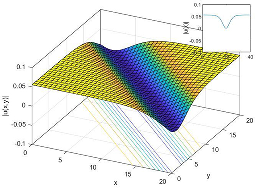
Figure 1. 2-D, 3-D, and contour plot of dark soliton solution Equation (20) when λ = 3, μ = 2, β = 0.6, α = 0.9, ε = 0.2, c = 0.3, t = 2, γ = 3 and z = 2 for 2-D.

FIGURE 2

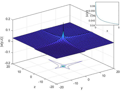
Figure 2. 2-D, 3-D, and contour plot of singular soliton solution Equation (21) when λ = 0.3, μ = 0, β = 0.6, α = 1/3, ε = 2, c = −0.3, t = 2, γ = 3 and z = 2 for 2-D.

FIGURE 3

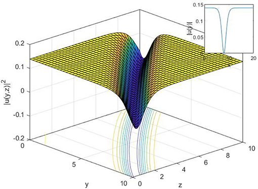
Figure 3. 2-D, 3-D, and contour plot of dark soliton solution Equation (22) when λ = 3, μ = 1, β = 0.1, α = 0.9, ε = 0.2, c = 0.3, t = 2, γ = 3, a₀ = 1, b₀ = 2 and z = 2 for 2-D.

FIGURE 4

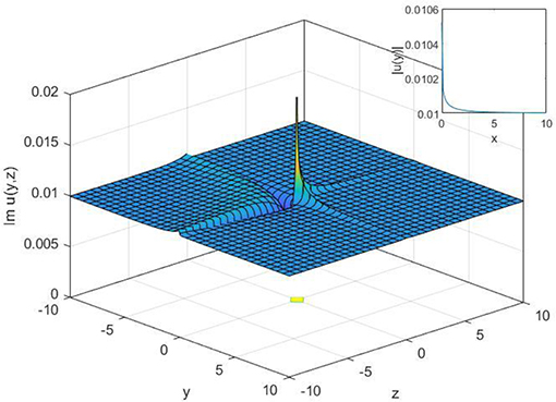
Figure 4. 2-D, 3-D, and contour plot of singular soliton solution Equation (23) when λ = 1, μ = 0, β = 0.6,$\alpha =\frac{1}{3},\epsilon =2,c=0.3,t=2,\gamma =0.3$, a₀ = 0.1, b₀ = 1 and z = 2 for 2-D.

FIGURE 5

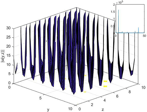
Figure 5. 2-D, 3-D, and contour plot of periodic singular soliton solution Equation (24) when λ = 0.1, μ = 0.3, β = 0.6, α = 0.9, ε = 0.1, c = 0.3, t = 2, γ = 0.3, a₀ = 0.5, b₁ = 0.2 and z = 2 for 2-D.

FIGURE 6

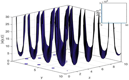
Figure 6. 2-D, 3-D, and contour plot of periodic singular soliton solution Equation (25) when λ = 1, μ = 1, β = 0.6, α = 0.9, ε = 0.1,c = 3, t = 2, γ = 3a₀ = 0.5, b₀ = 0.2 and z = 2 for 2-D.

FIGURE 7

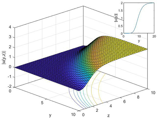
Figure 7. 2-D, 3-D, and contour plot of Equation (27), when t = 2, c = 3, γ = 2, α = 0.5, β = 0.6 and z = 2 for 2-D.

FIGURE 8

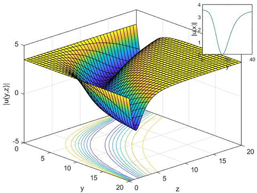
Figure 8. 2-D, 3-D, and contour plot of Equation (28), when t = 2, c = 3, γ = 0.2,$\alpha =\frac{1}{3},\beta =0.6$ and z = 2 for 2-D.

FIGURE 9

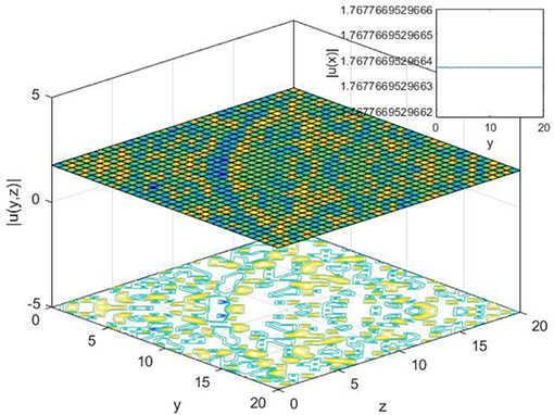
Figure 9. 2-D, 3-D, and contour plot of Equation (29), when t = 2, c = 0.3, γ = 0.2,α = 0.5, β = 0.6 and z = 2 for 2-D.

FIGURE 10

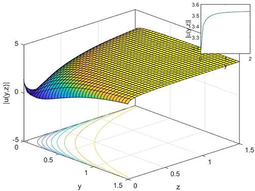
Figure 10. 2-D, 3-D, and contour plot of Equation (30), when t = 2, c = 0.3, γ = 0.2,α = 0.5, β = 0.6 and z = 2 for 2-D.

Data Availability Statement

The datasets generated for this study are available on request to the corresponding author.

Author Contributions

All authors listed have made a substantial, direct and intellectual contribution to the work, and approved it for publication.

Conflict of Interest

The authors declare that the research was conducted in the absence of any commercial or financial relationships that could be construed as a potential conflict of interest.

References

1. Oruç Ö, Bulut F, Esen A. Numerical solution of the KdV equation by Haar wavelet method. Pramana. (2016) 87:94. doi: 10.1007/s12043-016-1286-7

CrossRef Full Text | Google Scholar

2. Yousif MA, Mahmood BA, Ali KK, Ismael HF. Numerical simulation using the homotopy perturbation method for a thin liquid film over an unsteady stretching sheet. Int J Pure Appl Math. (2016) 107:289–300. doi: 10.12732/ijpam.v107i2.1

CrossRef Full Text | Google Scholar

3. Ismael HF, Ali KK. MHD casson flow over an unsteady stretching sheet. Adv Appl Fluid Mech. (2017) 20:533–41. doi: 10.17654/FM020040533

CrossRef Full Text

4. Bulut H, Ergüt M, Asil V, Bokor RH. Numerical solution of a viscous incompressible flow problem through an orifice by Adomian decomposition method. Appl Math Comput. (2004) 153:733–41. doi: 10.1016/S0096-3003(03)00667-2

CrossRef Full Text | Google Scholar

5. Ismael HF, Arifin NM. Flow and heat transfer in a maxwell liquid sheet over a stretching surface with thermal radiation and viscous dissipation. JP J Heat Mass Transf. (2018) 15:847–66. doi: 10.17654/HM015040847

CrossRef Full Text | Google Scholar

6. Ali KK, Ismael HF, Mahmood BA, Yousif MA. MHD Casson fluid with heat transfer in a liquid film over unsteady stretching plate. Int J Adv Appl Sci. (2017) 4:55–8. doi: 10.21833/ijaas.2017.01.008

CrossRef Full Text | Google Scholar

7. Ismael HF. Carreau-Casson fluids flow and heat transfer over stretching plate with internal heat source/sink and radiation. Int J Adv Appl Sci J. (2017) 6:81–6. doi: 10.21833/ijaas.2017.07.003

CrossRef Full Text | Google Scholar

8. Zeeshan, Ismael HF, Yousif MA, Mahmood T, Rahman SU. Simultaneous effects of slip and wall stretching/shrinking on radiative flow of magneto nanofluid through porous medium. J Magn. (2018) 23:491–8. doi: 10.4283/JMAG.2018.23.4.491

CrossRef Full Text | Google Scholar

9. Bulut H, Sulaiman TA, Baskonus HM, Aktürk T. On the bright and singular optical solitons to the (2 + 1)-dimensional NLS and the Hirota equations. Opt Quant Electron. (2018) 50:134. doi: 10.1007/s11082-018-1411-6

CrossRef Full Text | Google Scholar

10. Baskonus HM, Sulaiman TA, Bulut H. On the novel wave behaviors to the coupled nonlinear Maccari's system with complex structure. Optik. (2017) 131:1036–43. doi: 10.1016/j.ijleo.2016.10.135

CrossRef Full Text | Google Scholar

11. Baskonus HM, Bulut H, Sulaiman TA. New complex hyperbolic structures to the lonngren-wave equation by using sine-gordon expansion method. Appl Math Nonlinear Sci. (2019) 4:141–50. doi: 10.2478/AMNS.2019.1.00013

CrossRef Full Text | Google Scholar

12. Eskitaşçioglu EI, Aktaş MB, Baskonus HM. New complex and hyperbolic forms for ablowitz–kaup–newell–segur wave equation with fourth order. Appl Math Nonlinear Sci. (2019) 4:105–12. doi: 10.2478/AMNS.2019.1.00010

CrossRef Full Text | Google Scholar

13. Vakhnenko VO, Parkes EJ, Morrison AJ. A Bäcklund transformation and the inverse scattering transform method for the generalised Vakhnenko equation. Chaos Solitons Fract. (2003) 17:683–92. doi: 10.1016/S0960-0779(02)00483-6

CrossRef Full Text | Google Scholar

14. Cattani C, Sulaiman TA, Baskonus HM, Bulut H. On the soliton solutions to the Nizhnik-Novikov-Veselov and the Drinfel'd-Sokolov systems. Opt Quant Electron. (2018) 50:138. doi: 10.1007/s11082-018-1406-3

CrossRef Full Text | Google Scholar

15. Seadawy R, Kumar D, Chakrabarty AK. Dispersive optical soliton solutions for the hyperbolic and cubic-quintic nonlinear Schrödinger equations via the extended sinh-Gordon equation expansion method. Eur Phys Plus J. (2018) 133:182. doi: 10.1140/epjp/i2018-12027-9

CrossRef Full Text | Google Scholar

16. Bulut H, Sulaiman TA, Baskonus HM. Dark, bright optical and other solitons with conformable space-time fractional second-order spatiotemporal dispersion. Optik. (2018) 163:1–7. doi: 10.1016/j.ijleo.2018.02.086

CrossRef Full Text | Google Scholar

17. Manafian J, Lakestani M, Bekir A. Study of the analytical treatment of the (2+1)-dimensional zoomeron, the duffing and the SRLW equations via a new analytical approach. Int J Appl Comput Math. (2016) 2:243–68. doi: 10.1007/s40819-015-0058-2

CrossRef Full Text | Google Scholar

18. Hammouch Z, Mekkaoui T, Agarwal P. Optical solitons for the Calogero-Bogoyavlenskii-Schiff equation in (2 + 1) dimensions with time-fractional conformable derivative. Eur Phys Plus J. (2018) 133:248. doi: 10.1140/epjp/i2018-12096-8

CrossRef Full Text | Google Scholar

19. Dewasurendra M, Vajravelu K. On the method of inverse mapping for solutions of coupled systems of nonlinear differential equations arising in nanofluid flow, heat and mass transfer. Appl Math Nonlinear Sci. (2018) 3:1–14. doi: 10.21042/AMNS.2018.1.00001

CrossRef Full Text | Google Scholar

20. Ilhan OA, Esen A, Bulut H, Baskonus HM. Singular solitons in the pseudo-parabolic model arising in nonlinear surface waves. Results Phys. (2019) 12:1712:5. doi: 10.1016/j.rinp.2019.01.059

CrossRef Full Text | Google Scholar

21. Yokus, Baskonus HM, Sulaiman TA, Bulut H. Numerical simulation and solutions of the two-component second order KdV evolutionarysystem. Numer. Methods Partial Differ Equ. (2018) 34:211–27. doi: 10.1002/num.22192

CrossRef Full Text | Google Scholar

22. Cattani STA, Baskonus HM, Bulut H. Solitons in an inhomogeneous Murnaghan's rod. Eur Phys Plus J. (2018) 133:228. doi: 10.1140/epjp/i2018-12085-y

CrossRef Full Text | Google Scholar

23. Houwe A, Justin M, Jerome D, Betchewe G, Doka SY. TimoleonCrepin, K. Soliton solutions, kink and antikink of the Gerdjikov-Ivanov equation. Preprints 2018:2018090284 doi: 10.20944/preprints201809.0284.v1

CrossRef Full Text | Google Scholar

24. Yang X, Yang Y, Cattani C, Zhu CM. A new technique for solving the 1-D Burgers equation. Therm Sci. (2017) 21:S129–36. doi: 10.2298/TSCI17S1129Y

CrossRef Full Text | Google Scholar

25. Hammouch Z, Mekkaoui T. Traveling-wave solutions of the generalized Zakharov equation with time-space fractional derivatives. J MESA. (2014) 5:489–98. doi: 10.20944/preprints201903.0114.v1

CrossRef Full Text | Google Scholar

26. Baskonus HM, Yel G, Bulut H. Novel wave surfaces to the fractional Zakharov-Kuznetsov-Benjamin-Bona-Mahony equation. In: AIP Conference Proceedings. Istanbul (2017). doi: 10.1063/1.4992767

CrossRef Full Text | Google Scholar

27. Baskonus HM, Bulut H. Exponential prototype structures for (2+1)-dimensional Boiti-Leon-Pempinelli systems in mathematical physics. Waves Random Complex Media. (2016) 26:189–96. doi: 10.1080/17455030.2015.1132860

CrossRef Full Text | Google Scholar

28. Baskonus HM, Bulut H. An effective schema for solving some nonlinear partial differential equation arising in nonlinear physics. Open Phys. (2015) 13:280–89. doi: 10.1515/phys-2015-0035

CrossRef Full Text | Google Scholar

29. Bulut H. Application of the modified exponential function method to the Cahn-Allen equation. In: AIP Conference Proceedings. Istanbul (2017). doi: 10.1063/1.4972625

CrossRef Full Text | Google Scholar

30. Wei G, Ismael HF, Bulut H, Baskonus HM. Instability modulation for the (2+1)-dimension paraxial wave equation and its new optical soliton solutions in Kerr media. Phys Scr. (2019). doi: 10.1088/1402-4896/ab4a50

CrossRef Full Text | Google Scholar

31. Yang XF, Deng ZC, Wei Y. A riccati-bernoulli sub-ODE method for nonlinear partial differential equations and its application. Adv Differ Equat. (2015) 2015:117. doi: 10.1186/s13662-015-0452-4

CrossRef Full Text | Google Scholar

32. Manafian J, Foroutan M, Guzali A. Applications of the ETEM for obtaining optical soliton solutions for the Lakshmanan-Porsezian-Daniel model. Eur. Phys. Plus J. (2017) 132:494. doi: 10.1140/epjp/i2017-11762-7

CrossRef Full Text | Google Scholar

33. Biswas, Ekici M, Sonmezoglu A, Alqahtani RT. Optical solitons with differential group delay for coupled Fokas–Lenells equation by extended trial function scheme. Optik. (2018) 165:102–10. doi: 10.1016/j.ijleo.2018.03.102

CrossRef Full Text | Google Scholar

34. Li HM, Xu YS, Lin J. New optical solitons in high-order dispersive cubic-quintic nonlinear Schrodinger equation. Commun. Theor. Phys. (2004) 41:6. doi: 10.1088/0253-6102/41/6/829

CrossRef Full Text | Google Scholar

35. Jawad JM, Abu-AlShaeer MJ, Biswas A, Zhou Q, Moshokoa S, Belic M. Optical solitons to Lakshmanan-Porsezian-Daniel model for three nonlinear forms. Optik. (2018) 160:197–202. doi: 10.1016/j.ijleo.2018.01.121

CrossRef Full Text | Google Scholar

36. Yokuş A, Gülbahar S. Numerical solutions with linearization techniques of the fractional harry dym equation. Appl. Math. Nonlinear Sci. (2019) 4:35–42. doi: 10.2478/AMNS.2019.1.00004

CrossRef Full Text | Google Scholar

37. Baskonus H, Mekkaoui T, Hammouch Z, Bulut H. Active control of a chaotic fractional order economic system. Entropy. (2015) 17:5771–83. doi: 10.3390/e17085771

CrossRef Full Text | Google Scholar

38. Baskonus HM, Hammouch Z, Mekkaoui T, Bulut H. Chaos in the fractional order logistic delay system: circuit realization and synchronization. In: AIP Conference Proceedings. Greece (2016). doi: 10.1063/1.4952077

CrossRef Full Text | Google Scholar

39. Baskonus HM, Bulut H. On the numerical solutions of some fractional ordinary differential equations by fractional Adams-Bashforth-Moulton method. Open Math. (2015) 13:547–56. doi: 10.1515/math-2015-0052

CrossRef Full Text | Google Scholar

40. Esen A, Sulaiman TA, Bulut H, Baskonus HM. Optical solitons to the space-time fractional (1+ 1)-dimensional coupled nonlinear Schrödinger equation. Optik. (2018) 167:150–6. doi: 10.1016/j.ijleo.2018.04.015

CrossRef Full Text | Google Scholar

41. Subashini R, Ravichandran C, Jothimani K, Baskonus HM. Existence results of Hilfer integro-differential equations with fractional order. Discret. Contin. Dyn. Syst. (2019) 911:911–23. doi: 10.3934/dcdss.2020053

CrossRef Full Text | Google Scholar

42. Veeresha P, Prakasha DG, Baskonus HM. New numerical surfaces to the mathematical model of cancer chemotherapy effect in Caputo fractional derivatives. Chaos An Interdiscip. J Nonlinear Sci. (2019) 29:13119. doi: 10.1063/1.5074099

PubMed Abstract | CrossRef Full Text | Google Scholar

43. Yang AM, Zhang YZ, Cattani C, Xie GN, Rashidi MM, Zhou YJ, et al. Application of local fractional series expansion method to solve Klein-Gordon equations on cantor sets. Abstr Appl Anal. (2014) 2014:372741. doi: 10.1155/2014/372741

CrossRef Full Text | Google Scholar

44. Heydari MH, Hooshmandasl MR, Ghaini FMM, Cattani C. Wavelets method for solving fractional optimal control problems. Appl. Math. Comput. (2016) 286:139–54. doi: 10.1016/j.amc.2016.04.009

CrossRef Full Text | Google Scholar

45. Zhang Y, Cattani C, Yang J-X. Local fractional homotopy perturbation method for solving non-homogeneous heat conduction equations in fractal domains. Entropy. (2015) 170:6753–64. doi: 10.3390/e17106753

CrossRef Full Text | Google Scholar

46. Brzezinski DW. Review of numerical methods for NumILPT with computational accuracy assessment for fractional calculus. Appl Math Nonlinear Sci. (2019) 3:487–502. doi: 10.2478/AMNS.2018.2.00038

CrossRef Full Text | Google Scholar

47. Brzezinski DW. Comparison of fractional order derivatives computational accuracy-right hand vs left hand definition. Appl Math Nonlinear Sci. (2017) 2:237–48. doi: 10.21042/AMNS.2017.1.00020

CrossRef Full Text | Google Scholar

48. Machado JT, Kiryakova V, Mainardi F. Recent history of fractional calculus. Commun Nonlinear Sci Numer Simulat. (2011) 16:1140–53. doi: 10.1016/j.cnsns.2010.05.027

CrossRef Full Text | Google Scholar

49. Weyl H. Bemerkungen zum begriff des differentialquotienten gebrochener ordnung. Zürich. Naturf. Ges. (1917) 62:296–302.

50. Riesz M. L'intégrale de Riemann-Liouville et le problème de Cauchy pour l'équation des ondes. Bull. la Société Mathématique Fr. (1939) 67:153–70. doi: 10.24033/bsmf.1309

CrossRef Full Text | Google Scholar

51. Podlubny I. An introduction to fractional derivatives, fractional differential equations, to methods of their solution and some of their applications. Math. Sci. Eng. (1999) 198:24–340.

Google Scholar

52. Atangana A, Baleanu D. New fractional derivatives with non-local and non-singular kernel: Theory and application to heat transfer model. Therm. Sci. (2016) 20:763–69. doi: 10.2298/TSCI160111018A

CrossRef Full Text | Google Scholar

53. Miller S, Ross B. An Introduction to the Fractional Calculus and Fractional Differential Equations. New York, NY: Wiley (1993).

54. Khalil R, Al Horani M, Yousef A, Sababheh M. A new definition of fractional derivative. J Comput Appl Math. (2014) 264:65–70. doi: 10.1016/j.cam.2014.01.002

CrossRef Full Text | Google Scholar

55. Atangana A, Baleanu D, Alsaedi A. New properties of conformable derivative. Open Math. (2015) 13:889–98. doi: 10.1515/math-2015-0081

CrossRef Full Text | Google Scholar

56. Sousa JVC, Oliveira EC. A new truncated M-fractional derivative type unifying some fractional derivative types with classical properties. Int. J. Anal. Appl. (2018) 16:83–96.

Google Scholar

57. Choi S, Howell JC. Paraxial ray optics cloaking. Opt. Exp. (2014) 22:29465–78. doi: 10.1364/OE.22.029465

PubMed Abstract | CrossRef Full Text | Google Scholar