Jacobi Spectral Galerkin Method for Distributed-Order Fractional Rayleigh–Stokes Problem for a Generalized Second Grade Fluid

1. Introduction

Let Λ ⊂ ℝ^d (d = 1, 2) be a bounded convex domain with a polygonal boundary ∂Λ, and ${T}>0$ be a fixed time. The purpose of this paper is to extend the approach in Hafez and Zaky [1] to the distributed-order time-fractional Rayleigh-Stokes problem for a generalized second-grade fluid in one and two space dimensions. The mathematical model is given by

$\begin{array}{ll}\begin{array}{c}{\partial }_{t}U(\text{x},t)-\left(1+0D_t^{w(\nu )}\right)\Delta U(\text{x},t)=H(\text{x},t),\text{x}\in \Lambda ,t\in (0,{T}],\end{array}& (1)\end{array}$

with initial-boundary conditions:

$\begin{array}{ll}\begin{array}{c}U(\text{x},0)=f(\text{x}),\text{x}\in \Lambda ,\end{array}& (2)\end{array}$

$\begin{array}{ll}\begin{array}{c}U(\text{x},t){|}_{\text{x}\in \partial \Lambda }=g(\text{x},t),t\in (0,{T}],\end{array}& (3)\end{array}$

where Δ is the Laplacian operator, ∂Λ is the boundary of Λ, H(x, t), f(x), and g(x, t) are given smooth functions on Λ. The distributed-order fractional derivative $0D_t^{w(\nu )}$ is defined by

$\begin{array}{ll}{}_0{D}_t^{w(\nu )}U(x,t)={\displaystyle {\int }_0^{1}w(\nu ){}_0^C{D}_t^{1-\nu }U(x,t)d\nu },& (4)\end{array}$

where w(ν) is a non-negative smooth weight function satisfying the conditions

$\begin{array}{l}w(\nu )\ge 0,w(\nu )\not\equiv 0,{\displaystyle {\int }_0^1}w(\nu )d\nu <\infty ,\\ 0^C{D}_t^{\nu }U(\text{x},t)=\frac{\text{1}}{\Gamma \text{(1 -}\nu \text{)}}{\displaystyle {\int }_0^t}{(t-\xi )}^{-\nu }\frac{\partial U(\text{x},\xi )}{\partial \xi }d\xi ,0<\nu <1.& (5)\end{array}$

The fractional-order derivatives appearing in (4) is defined in the Caputo sense. Unlike Riemann-Liouville derivatives, Caputo derivatives are not singular on the domain boundaries. That feature makes them particularly appealing for non-local numerical methods, like the spectral methods. Zhang et al. [2] have also confirmed that Riemann-Liouville derivatives could cause mass-balance errors on bounded domains. The time derivative is thus defined in the Caputo sense.

Recently, the fractional-order Rayleigh-Stokes problem has received considerable attention in recent years. This model plays an important role in describing the behavior of some non-Newtonian fluids [3, 4]. In order to gain insights into the behavior of the solution of this model, there has been substantial interest in deriving a closed form solution for the special case w(ν) = δ(ν − 1 + β), where δ(·) is the Dirac delta function and β ∈ (0, 1). For example, Shen et al. [4] derived exact solutions of this model using the Fourier transform and the fractional Laplace transform. Girault and Saadouni [5] analyzed the existence and uniqueness of a weak solution of a closely related time-dependent grade-two fluid model. Zhao and Yang [6] obtained exact solutions using the eigenfunction expansion. Xue and Nie [7] obtained also closed form solutions of this model in a porous half-space using both Fourier and fractional Laplace transforms. The exact solutions obtained in these studies involve infinite series and special functions, e.g., generalized Mittag-Leffler functions, and thus are inconvenient for numerical evaluation. Further, closed-form solutions are available only for a restricted class of problem settings. Hence, it is imperative to develop efficient and optimally accurate numerical algorithms for problem (1). Wu [8] developed an implicit numerical scheme by transforming the above mentioned problem into an integral equation. Lin and Jiang [9] introduced a numerical sachem based on the reproducing kernel space. Mohebbi et al. [10] compared a fourth-order compact scheme with radial basis functions meshless approach. Recently, Bazhlekova et al. [11] developed two fully discrete schemes based on the backward difference method and backward Euler method and a semidiscrete scheme based on the Galerkin finite element method. Abdelkawy and Alqahtani [12] proposed spectral collocation techniques for solving fractional Stokes' first problem for a heated generalized second grade fluid. Bhrawy et al. [13] developed two shifted Jacobi-Gauss collocation schemes. More recently, Dehghan and Abbaszadeh [14] developed a finite element method for two-dimensional fractional Rayleigh–Stokes model on complex geometries. Shivanian and Jafarabadi [15] developed a spectral meshless radial point nterpolation technique. Zaky [16] develop efficient algorithms based on the Legendre-tau approximation for one- and two-dimensional fractional Rayleigh–Stokes problems for a generalized second-grade fluid. Yang and Jiang [17] proposed a numerical algorithm based on the L1 finite difference scheme for the temporal direction while the Legendre spectral method for the spatial direction.

Theoretical studies on numerical methods for fractional differential equations involving distributed-order derivatives have received considerable attention in the last decade [18–20]. A general form of distributed-order fractional ordinary differential equation is solved in Katsikadelis [21], Mashayekhi and Razzaghi [22], and Zaky et al. [23]. Numerical methods for solving distributed-order time-fractional diffusion equations are presented in Morgado and Rebelo [24], Abdelkawy et al. [25], and Zaky and Machado [26]. Numerical methods for distributed-order space-fractional diffusion equations are provided in Abbaszadeh [27], Kazmi and Khaliq [28], and Fan and Liu [29]. Numerical methods for multi-dimensional distributed-order generalized Schrödinger equations are provided in Bhrawy and Zaky [30]. For numerical methods for solving distributed-order fractional optimal control problems, see [31, 32]. In this paper, we use a non-local representation of the solution of the distributed-order time-fractional Rayleigh-Stokes problem to introduce spectral solutions. The spectral and pseudospectral methods are well-known for their high accuracy and have been used extensively in scientific computation, see [33–41] and the references therein. The main contribution of this paper is to develop Jacobi-Galerkin algorithms for solving the multidimensional distributed-order time-fractional Rayleigh-Stokes problem (1).

The outline of this work is as follows. In section 2, we introduce the distributed-order fractional differentiation matrix of the shifted Jacobi polynomials. In section 3, we derive a time-space discretization for the one-dimensional distributed-order fractional Rayleigh–Stokes problem. In section 4, we consider the numerical solution of the two-dimensional case. In section 5, we present various numerical results exhibiting the efficiency of our numerical schemes. We end this paper with a few concluding remarks in section 6.

2. Distribute-Order Fractional Differentiation Matrix

In this section, we first introduce some basic properties of Jacobi polynomials. Then, we construct the operational matrix of distributed-order fractional derivative for the Jacobi polynomials. The Jacobi polynomials $J_i^{(\gamma ,\eta )}(z);\gamma >-1,\eta >-1,z\in (-1,1)$ are defined by the following three term recurrence relation:

$\begin{array}{l}{J}_{i+1}^{(\gamma ,\eta )}(z)=({\tilde{R}}_{i}z-{\tilde{B}}_i)J_i^{(\gamma ,\eta )}(z)-{\tilde{C}}_i{J}_{i-1}^{(\gamma ,\eta )}(z),i\ge 1,\end{array}$

with

$\begin{array}{l}{J}_0^{(\gamma ,\eta )}(z)=1,J_1^{(\gamma ,\eta )}(z)=\frac{1}{2}(\eta +\gamma +2)z+\frac{1}{2}(-\eta +\gamma ),\end{array}$

where

$\begin{array}{l}\begin{array}{c}{\tilde{R}}_i=\frac{(\gamma +\eta +2i+1)(\gamma +2i+\eta +2)}{2(1+i)(\gamma +i+\eta +1)},\\ {\tilde{B}}_i=\frac{(\gamma +\eta +2i+1)({\eta }^2-{\gamma }^2)}{2(1+i)(\gamma +i+\eta +1)(\gamma +2i+\eta )},\\ {\tilde{C}}_i=\frac{(\gamma +\eta +2i+2)(\gamma +i)(i+\eta )}{(1+i)(\gamma +i+\eta +1)(\gamma +2i+\eta )}.\end{array}\end{array}$

Using the linear map $z=\frac{2x}{L}-1$, the interval [−1, 1] can be rescaled onto [0, L]. Hence, the set of shifted Jacobi polynomials $J_{L,i}^{(\gamma ,\eta )}(x);x\in \left[0,L\right]$ can be generated by:

$\begin{array}{l}{J}_{L,i+1}^{(\gamma ,\eta )}(x)=({\tilde{E}}_{i}x-{\tilde{K}}_i)J_{L,i}^{(\gamma ,\eta )}(x)-{\tilde{C}}_i{J}_{L,i-1}^{(\gamma ,\eta )}(x),i\ge 1,\end{array}$

where

$\begin{array}{l}{\tilde{E}}_i=\frac{(\gamma +2i+\eta +1)(2+\gamma +2i+\eta )}{L(1+i)(1+i+\gamma +\eta )},\\ {\tilde{K}}_i=\frac{(\gamma +2i+\eta +1)(2i^2+(\eta +1)(\gamma +\eta )+2i(\gamma +1+\eta ))}{(1+i)(1+i+\gamma +\eta )(\gamma +2i+\eta )}.\end{array}$

The terminal values of the shifted Jacobi polynomials satisfy

$\begin{array}{ll}{J}_{L,i}^{(\gamma ,\eta )}(0)={(-1)}^i\frac{\Gamma (1+i+\eta )}{\Gamma (1+\eta )i!},J_{L,i}^{(\gamma ,\eta )}(L)=\frac{\Gamma (1+i+\gamma )}{\Gamma (1+\gamma )i!},& (6)\end{array}$

The $J_{L,j}^{(\gamma ,\eta )}(x)$ satisfies the following orthogonality relation

$\begin{array}{ll}{\displaystyle {\int }_0^L}{J}_{L,j}^{(\gamma ,\eta )}(x)J_{L,i}^{(\gamma ,\eta )}(x)w_L^{(\gamma ,\eta )}(x)dx={\delta }_{ji}{h}_{L,i}^{(\gamma ,\eta )},& (7)\end{array}$

where $w_L^{(\gamma ,\eta )}(x)=x^{\eta }{(L-x)}^{\gamma }$ is the weight function, and

$\begin{array}{ll}{h}_{L,i}^{(\gamma ,\eta )}=\frac{L^{1+\gamma +\eta }\Gamma (i+1+\gamma )\Gamma (i+1+\eta )}{(2i+1+\gamma +\eta )i!\Gamma (i+1+\gamma +\eta )}.& (8)\end{array}$

The following Jacobi-Gauss quadrature rule is commonly used to approximate the previous integrals

$\begin{array}{ll}{\displaystyle {\int }_0^L}\phi (x)w_L^{(\gamma ,\eta )}(x)dx={\displaystyle \sum _{i=0}^N}{\varpi }_{G,L,i}^{(\gamma ,\eta )}\phi (x_{G,L,i}^{(\gamma ,\eta )}),\forall \phi \in P_{2N+1}(\Lambda ),& (9)\end{array}$

where P_N(Λ) is any sequence of polynomials of degree not exceeding N, ${\varpi }_{G,L,i}^{(\gamma ,\eta )}$ and $x_{G,L,i}^{(\gamma ,\eta )}(0\le i\le N)$ are the shifted Jacobi Gauss wights and nodes in Λ, respectively.

For the shifted Jacobi-Gauss: The weights are given by

$\begin{array}{ll}{\varpi }_{G,L,i}^{(\gamma ,\eta )}=\frac{C_{L,N}^{(\gamma ,\eta )}}{(L-x_{G,L,i}^{(\gamma ,\eta )})x_{G,L,i}^{(\gamma ,\eta )}{\left[{\partial }_x{J}_{N+1}^{(\gamma ,\eta )}(x_{G,L,i}^{(\gamma ,\eta )})\right]}^2},0\le i\le N,& (10)\end{array}$

where

$\begin{array}{l}{C}_{L,N}^{(\gamma ,\eta )}=\frac{L^{\gamma +\eta +1}\Gamma (N+\gamma +2)\Gamma (N+\eta +2)}{(N+1)!\Gamma (N+\gamma +\eta +2)},\end{array}$

and the nodes $x_{G,L,i}^{(\gamma ,\eta )}(0\le i\le N)$ are the zeros of $J_{L,N+1}^{(\gamma ,\eta )}(x).$

Lemma 2.1. (see [42]) The q times differentiation of the Jacobi polynomials $J_{L,j}^{(\gamma ,\eta )}(x)$ are given by

$\begin{array}{ll}{D}^q{J}_{L,j}^{(\gamma ,\eta )}(x)={\displaystyle \sum _{i=0}^{j-q}}{A}_q(j,i,\gamma ,\eta )J_{L,i}^{(\gamma ,\eta )}(x),q\in {\mathbb{N}}^{+},& (11)\end{array}$

where

$\begin{array}{l}{A}_q(j,i,\gamma ,\eta )=\frac{{(\lambda +j)}_q{(j+q+\lambda )}_i{(q+1+i+\gamma )}_{j-i-q}\Gamma (i+\lambda )}{L^q(j-q-i)!\Gamma (\lambda +2i)}\\ {\times }_3{F}_2\left(\begin{array}{cccc}q+i-j,& i+q+\lambda +j,& 1+i+\gamma & \\ & & & ;1\\ q+i+1+\gamma ,& 2i+1+\lambda & & \end{array}\right),& (12)\end{array}$

where (·)_i is the Pochhammer symbol, λ = γ + η + 1, and ₃F₂ is the generalized hypergeometric function.

Lemma 2.2. (see [43]) The Caputo fractional derivative of order ν ∈ (0, 1) of the shifted Jacobi polynomials is given by

$\begin{array}{ll}{}_0{}^{C}D{}_x^{\nu }{J}_{L,i}^{(\gamma ,\eta )}(x)\approx {\displaystyle \sum _{j=0}^{N}G}(i,j,\gamma ,\eta ,\nu )J_{L,j}^{(\gamma ,\eta )}(x),i=1,\cdots ,N,& (13)\end{array}$

where ${G}(i,j,\gamma ,\eta ,\nu )=\sum _{k=1}^i{\theta }_{ijk},$ and

$\begin{array}{l}{\theta }_{ijk}=\frac{\begin{array}{c}{(-1)}^{i-k}{L}^{\gamma +\eta -\nu +1}\Gamma (1+j+\eta )\\ \Gamma (1+i+\eta )\Gamma (1+k+\gamma +i+\eta )\end{array}}{\begin{array}{c}{h}_{L,j}^{(\gamma ,\eta )}\Gamma (\eta +j+\gamma +1)\Gamma (\eta +k+1)(i-k)!\\ \Gamma (\eta +i+\gamma +1)\Gamma (k+1-\nu )\end{array}}\\ \times {\displaystyle \sum _{\ell =0}^j}\frac{\begin{array}{c}{(-1)}^{j-\ell }\Gamma (j+\ell +1+\gamma +\eta )\Gamma (1+\gamma )\\ \Gamma (\ell +k-\nu +\gamma +\ell +1)\end{array}}{\begin{array}{c}\Gamma (\ell +1+\eta )(\ell )!(j-\ell )!\\ \Gamma (\ell +2+\gamma +k-\nu +\ell )\end{array}}.& (14)\end{array}$

Lemma 2.3. Let $x_{G,L,r}^{(0,0)}$ and ${\varpi }_{G,L,r}^{(0,0)}(0\le r\le N)$ be the set of nodes and the weights of the Legendre-Gauss quadrature formula given in (10). Then, the distributed-order fractional derivative of the shifted Jacobi polynomials is given by

$\begin{array}{ll}{}_0{D}_t^{w(\nu )}{J}_{L,i}^{(\gamma ,\eta )}(x)\approx {\displaystyle \sum _{j=0}^N{\widehat{A}}_{\omega }}(i,j,\gamma ,\eta )J_{L,j}^{(\gamma ,\eta )}(x),i=1,\dots ,N,& (15)\end{array}$

where

$\begin{array}{l}{\widehat{A}}_{\omega }(i,j,\gamma ,\eta )={\displaystyle \sum _{r=0}^N}\omega (x_{G,L,r}^{(0,0)}){\varpi }_{G,L,r}^{(0,0)}{G}\left(i,j,\gamma ,\eta ,1-x_{G,L,r}^{(0,0)}\right).\end{array}$

3. One-Dimensional Case

We consider the following one-dimensional distributed-order fractional Rayleigh–Stokes problem:

$\begin{array}{ll}{\partial }_{t}U(x,t)-\left(1{+}_0{D}_t^{w(\nu )}\right){\partial }_x^{2}U(x,t)=H(x,t),(x,t)\in \Omega :=\Lambda \times I,& (16)\end{array}$

$\begin{array}{l}U(x,0)=0,\\ U(0,t)=U(L,t)=0.& (17)\end{array}$

Let P_N(Λ) and P_M(I) denote the set of polynomials of degree N in space and M in time, respectively. Since we have the homogeneous initial and boundary conditions, we choose appropriate basis for the space ansatz from

$\begin{array}{ll}{P}_N^s(\Lambda )=\left\{U\in P_N(\Lambda )|U(0)=U(L)=0\right\},& (18)\end{array}$

as well as for time

$\begin{array}{ll}{P}_M^t(I)=\left\{U\in P_M(I)|U(0)=0\right\}.& (19)\end{array}$

For the sake of clarity, we define the multiindex L = (N, M) and

$\begin{array}{ll}\begin{array}{c}{W}_L:=P_M^t(I)\otimes P_N^s(\Lambda ),\\ S_L:=P_M(I)\otimes P_N(\Lambda ).\end{array}& (20)\end{array}$

To simplify the notation, we introduce the following integral operators for the Jacobi–Galerkin spectral formulation:

$\begin{array}{l}\langle \langle \langle ·\rangle \rangle \rangle \equiv {\displaystyle {\int }_0^L}{\displaystyle {\int }_0^L}{\displaystyle {\int }_0^{{T}}}·w_L^{(\gamma ,\eta )}(x)w_L^{(\gamma ,\eta )}(y)w_{{T}}^{(\gamma ,\eta )}(t)dxdydt,\\ \langle \langle ·\rangle \rangle \equiv {\displaystyle {\int }_0^L}{\displaystyle {\int }_0^{{T}}}·w_L^{(\gamma ,\eta )}(x)w_{{T}}^{(\gamma ,\eta )}(t)dxdt,\\ {\langle ·\rangle }_x\equiv {\displaystyle {\int }_0^L}·w_L^{(\gamma ,\eta )}(x)dx,\\ {\langle ·\rangle }_t\equiv {\displaystyle {\int }_0^{{T}}}·w_{{T}}^{(\gamma ,\eta )}(t)dt.& (21)\end{array}$

The spectral-Galerkin approximation of the solution U ∈ W_L is given by

$\begin{array}{ll}U(x,t)\simeq \widehat{U}(x,t)={\displaystyle \sum _{i=0}^{N-2}}{\displaystyle \sum _{j=0}^{M-1}}{\theta }_{L,i}^{(\gamma ,\eta )}(x){\text{U}}_{ij}{\vartheta }_{{T},j}^{(\gamma ,\eta )}(t),& (22)\end{array}$

where ${\theta }_{L,i}^{(\gamma ,\eta )}(x)\in P_N^s(\Lambda ),$ ${\vartheta }_{{T},j}^{(\gamma ,\eta )}(t)\in P_M^t(I)$, and U_ij are the unknown coefficients. The key idea behind the Galerkin approximation is to fined $\widehat{U}\in W_L$ such that

$\begin{array}{ll}\begin{array}{c}\langle \langle \widehat{Y}{\partial }_t\widehat{U}\rangle \rangle -\langle \langle {\widehat{Y}}_0{D}_t^{w(\nu )}({\partial }_x^2\widehat{U})\rangle \rangle -\langle \langle \widehat{Y}{\partial }_x^2\widehat{U}\rangle \rangle =\langle \langle H\widehat{Y}\rangle \rangle ,\forall \widehat{Y}\in W_L.\end{array}& (23)\end{array}$

The actual linear system for (23) depends on the choice of basis functions of W_L. We shall construct below suitable spectral basis functions ${\theta }_{L,i}^{(\gamma ,\eta )}(x)$ and ${\vartheta }_{{T},j}^{(\gamma ,\eta )}(t)$ of W_L. Therefore, we construct basis functions using compact combinations of the Jacobi polynomials. In this case, we define

$\begin{array}{l}{\theta }_{L,i}^{(\gamma ,\eta )}(x)=J_{L,i}^{(\gamma ,\eta )}(x)+{\kappa }_i{J}_{L,i+1}^{(\gamma ,\eta )}(x)+{\lambda }_i{J}_{L,i+2}^{(\gamma ,\eta )}(x),\\ {\vartheta }_{{T},j}^{(\gamma ,\eta )}(t)=J_{{T},j}^{(\gamma ,\eta )}(t)+{\mu }_j{J}_{{T},j+1}^{(\gamma ,\eta )}(t),& (24)\end{array}$

where the parameters μ_j, κ_i and λ_i are chosen to satisfy the boundary conditions in (17). Such basis functions are referred to as modal basis functions. (11).

Lemma 3.1. (see [1]) For all i, j ≥ 0, there exists a unique set of {κ_i, λ_i, μ_j} such that

$\begin{array}{l}{\theta }_{L,i}^{(\gamma ,\eta )}(x)=J_{L,i}^{(\gamma ,\eta )}(x)+{\kappa }_i{J}_{L,i+1}^{(\gamma ,\eta )}(x)+{\lambda }_i{J}_{L,i+2}^{(\gamma ,\eta )}(x),\\ {\vartheta }_{{T},j}^{(\gamma ,\eta )}(t)=J_{{T},j}^{(\gamma ,\eta )}(t)+{\mu }_j{J}_{{T},j+1}^{(\gamma ,\eta )}(t),& (25)\end{array}$

verify the boundary conditions in (17).

The set of basis functions ${\theta }_{L,i}^{(\gamma ,\eta )}(x)\in P_{N+2}^s(\Lambda )$ and ${\vartheta }_{{T},j}^{(\gamma ,\eta )}(t)\in P_{M+1}^t(I)$ are linearly independent. Hence, by dimension argument, we obtain

$\begin{array}{ll}\begin{array}{c}{P}_M^t(I)=\text{span}\left\{{\vartheta }_{{T},j}^{(\gamma ,\eta )}(t):j=0,1,2,\dots ,M-1\right\},\\ P_N^s(\Lambda )=\text{span}\left\{{\theta }_{L,i}^{(\gamma ,\eta )}(x):i=0,1,2,\dots ,N-2\right\}.\end{array}& (26)\end{array}$

It is clear that the Galerkin formulation of (23) is equivalent to following discrete discretization

$\begin{array}{l}\langle \langle {\theta }_{L,i}^{(\gamma ,\eta )}(x){\partial }_t\widehat{U}(x,t){\vartheta }_{{T},j}^{(\gamma ,\eta )}(t)\rangle \rangle \\ -\langle \langle {\theta }_{L,i}^{(\gamma ,\eta )}{(x)}_0{D}_t^{w(\nu )}({\partial }_x^2\widehat{U}(x,t)){\vartheta }_{{T},j}^{(\gamma ,\eta )}(t)\rangle \rangle \\ -\langle \langle {\theta }_{L,i}^{(\gamma ,\eta )}(x){\partial }_x^2\widehat{U}(x,t){\vartheta }_{{T},j}^{(\gamma ,\eta )}(t)\rangle \rangle =\langle \langle {\theta }_{L,i}^{(\gamma ,\eta )}(x)H(x,t){\vartheta }_{{T},j}^{(\gamma ,\eta )}(t)\rangle \rangle ,& (27)\end{array}$

for 0 ≤ j ≤ M − 1 and 0 ≤ i ≤ N − 2. Throughout this paper, we assume that the indices j and s vary between 0 and M − 1 and that the indices i and r vary between 0 and N − 2. Moreover, we assume that repeated indices are summed over. Thus, the matrix form of (27) becomes

$\begin{array}{l}{\langle {\theta }_{L,i}^{(\gamma ,\eta )}{\theta }_{L,r}^{(\gamma ,\eta )}\rangle }_x{U}_{ij}{\langle \frac{d{\vartheta }_{T,j}^{(\gamma ,\eta )}}{dt}{\vartheta }_{T,s}^{(\gamma ,\eta )}\rangle }_t\\ -{\langle {\theta }_{L,i}^{(\gamma ,\eta )}\frac{d^2{\theta }_{L,r}^{(\gamma ,\eta )}}{d{x}^2}\rangle }_x{U}_{ij}{\langle {}_0{D}_t^{w(\nu )}{\vartheta }_{T,j}^{(\gamma ,\eta )}{\vartheta }_{T,s}^{(\gamma ,\eta )}\rangle }_t& (28)\\ -{\langle {\theta }_{L,i}^{(\gamma ,\eta )}\frac{d^2{\theta }_{L,r}^{(\gamma ,\eta )}}{d{x}^2}\rangle }_x{U}_{ij}{\langle {\vartheta }_{T,j}^{(\gamma ,\eta )}{\vartheta }_{T,s}^{(\gamma ,\eta )}\rangle }_t\\ =\langle \langle {\theta }_{L,i}^{(\gamma ,\eta )}(x)H(x,t){\vartheta }_{T,j}^{(\gamma ,\eta )}(t)\rangle \rangle .\end{array}$

Let us denote

$\begin{array}{l}\begin{array}{c}\text{U}=({\text{U}}_{ij}),\text{H}=({\text{H}}_{ij}),\text{A}=({\text{A}}_{ir}),\text{B}=({\text{B}}_{ir}),\text{C}=({\text{C}}_{js}),\\ {\text{D}}_{\omega }=({\text{D}}_{js}^{\omega }),\text{E}=({\text{E}}_{js}),\text{H}=({\text{H}}_{js}),\end{array}\end{array}$

where H is the matrix whose entries are ${\mathbf{\text{H}}}_{ij}=\langle \langle {\theta }_{L,i}^{(\gamma ,\eta )}(x)H(x,t){\vartheta }_{{T},j}^{(\gamma ,\eta )}(t)\rangle \rangle$, U is the matrix of unknown coefficients, and the non-zero elements of the matrices A, B, C, D_ω and E are given explicitly by Theorem 0.0.5. The previous integrals can be computed using the Jacobi-Gauss quadrature rule (9). The discretization of the distributed-order fractional Rayleigh–Stokes problem (16) is equivalent to the following matrix equation

$\begin{array}{ll}\text{A}\text{U}\text{C}-\text{B}\text{U}{\text{D}}_{\omega }-\text{B}\text{U}\text{E}=\text{H}.& (29)\end{array}$

In order to be able to solve (29), we shall recast it in a more convenient form. To do so, we make use of the Kronecker product (represented by ⊗). If we consider the matrices H ∈ ℝ^n,m and G ∈ ℝ^q,p, then the Kronecker product of H and G is defined as follows

$\begin{array}{l}\text{H}\otimes \text{G}=\left(\begin{array}{cccc}{h}_{11}\text{G}& h_{12}\text{G}& \cdots & h_{1m}\text{G}\\ h_{21}\text{G}& h_{22}\text{G}& \cdots & h_{2m}\text{G}\\ ⋮& ⋮& \ddots & ⋮\\ h_{n1}\text{G}& h_{n2}\text{G}& \cdots & h_{nm}\text{G}\\ \end{array}\right)\in {ℝ}^{nq,mp}.\end{array}$

Let $h_i\in {ℝ}^n$ denote the columns of H ∈ ℝ^n,m so that H = [h₁, …, h_m]. Then vec(H) is defined to be the nm-vector formed by stacking the columns of H on top of one another, i.e.,

$\begin{array}{l}\text{vec}(H)=\left[\begin{array}{l}{h}_1\\ ⋮\\ h_m\end{array}\right]h_m\in {\text{ℝ}}^{nm}\end{array}$

The Kronecker product has the useful property that for any three matrices H, G and H for which the matrix product is defined, we have:

$\begin{array}{l}\text{vec}(\text{H}\text{G}\text{F})=({\text{F}}^T\otimes \text{H})\text{vec}(\text{G}),\end{array}$

where ^T denotes the transpose. Equation (29) can finally be expressed in matrix form as follows:

$\begin{array}{ll}\left({\text{C}}^T\otimes \text{A}-{\text{D}}_{\omega }^T\otimes \text{B}-{\text{E}}^T\otimes \text{B}\right)\text{vec}(\text{U})=\text{vec}(\text{H}).& (30)\end{array}$

Theorem 3.2. Let

$\begin{array}{l}{A}_{ir}={\langle {\theta }_{L,i}^{(\gamma ,\eta )}{\theta }_{L,r}^{(\gamma ,\eta )}\rangle }_x,B_{ir}={\langle {\theta }_{L,i}^{(\gamma ,\eta )}\frac{d^2{\theta }_{L,r}^{(\gamma ,\eta )}}{d{x}^2}\rangle }_x,\\ C_{js}={\langle \frac{d{\vartheta }_{T,j}^{(\gamma ,\eta )}}{dt}{\vartheta }_{T,s}^{(\gamma ,\eta )}\rangle }_t,D_{js}^{\omega }={\langle {}_0{D}_t^{w(\nu )}{\vartheta }_{T,j}^{(\gamma ,\eta )}{\vartheta }_{T,s}^{(\gamma ,\eta )}\rangle }_t,& (31)\\ E_{js}={\langle {\vartheta }_{T,j}^{(\gamma ,\eta )}{\vartheta }_{T,s}^{(\gamma ,\eta )}\rangle }_t.\end{array}$

Then the non-zero elements ${\mathbf{\text{A}}}_{ir},{\mathbf{\text{B}}}_{ir},{\mathbf{\text{C}}}_{js},{\mathbf{\text{D}}}_{js}^{\omega }$, and E_js are given by

$\begin{array}{l}{A}_{ii}=h_{L,i}^{(\gamma ,\eta )}+{\kappa }_i^2{h}_{L,i+1}^{(\gamma ,\eta )}+{\lambda }_i^2{h}_{L,i+2}^{(\gamma ,\eta )},\\ A_{i+1,i}=A_{i,i+1}={\kappa }_i{h}_{L,i+1}^{(\gamma ,\eta )}+{\lambda }_i{\kappa }_{i+1}{h}_{L,i+2}^{(\gamma ,\eta )},& (32)\\ A_{i+2,i}=A_{i,i+2}={\lambda }_i{h}_{L,i+2}^{(\gamma ,\eta )},\end{array}$

$\begin{array}{l}{B}_{ii}={\lambda }_i{A}_2(i+2,i,\gamma ,\eta )h_{L,i}^{(\gamma ,\eta )},\\ B_{ir}=O_2(r,i,\gamma ,\eta )h_{L,i}^{(\gamma ,\eta )}+O_2(r,i+1,\gamma ,\eta ){\kappa }_i{h}_{L,i+1}^{(\gamma ,\eta )}& (33)\\ +O_2(r,i+2,\gamma ,\eta ){\lambda }_i{h}_{L,i+2}^{(\gamma ,\eta )},r=i+n,n\ge 1,\end{array}$

$\begin{array}{l}{C}_{jj}={\mu }_j{A}_1(j+1,j,\gamma ,\eta )h_{{T},j}^{(\gamma ,\eta )},\\ C_{js}={\chi }_1(s,j,\gamma ,\eta )h_{{T},j}^{(\gamma ,\eta )}+{\chi }_1(s,j+1,\gamma ,\eta ){\mu }_j{h}_{{T},j+1}^{(\gamma ,\eta )},& (34)\\ s=j+n,n\ge 1,\end{array}$

$\begin{array}{l}{D}_{js}^{\omega }=({\widehat{A}}_{\omega }(s,j,\gamma ,\eta )+{\mu }_s{\widehat{A}}_{\omega }(s+1,j,\gamma ,\eta ))h_{{T},j}^{(\gamma ,\eta )}\\ +{\mu }_j({\widehat{A}}_{\omega }(s,j+1,\gamma ,\eta )+{\mu }_s{\widehat{A}}_{\omega }(s+1,j+1,\gamma ,\eta ))h_{{T},j+1}^{(\gamma ,\eta )},& (35)\end{array}$

$\begin{array}{ll}{E}_{jj}=h_{{T},j}^{(\gamma ,\eta )}+{\mu }_j^2{h}_{{T},j+1}^{(\gamma ,\eta )},& (36)\\ E_{j+1,j}=E_{j,j+1}={\mu }_j{h}_{{T},j+1}^{(\gamma ,\eta )},\end{array}$

where

$\begin{array}{l}{O}_{\sigma }(r,i,\gamma ,\eta )=A_{\sigma }(r,i,\gamma ,\eta )+{\kappa }_r{A}_{\sigma }(r+1,i,\gamma ,\eta )\\ +{\lambda }_r{A}_{\sigma }(r+2,i,\gamma ,\eta ),& (37)\end{array}$

$\begin{array}{ll}{\chi }_{\sigma }(s,j,\gamma ,\eta )=A_{\sigma }(s,j,\gamma ,\eta )+{\mu }_s{A}_{\sigma }(s+1,j,\gamma ,\eta ),& (38)\end{array}$

and $h_{L,i}^{(\gamma ,\eta )}$ is given by (8).

Proof. We shall only determine the non-zero elements of A as the proof for the non-zero entries of the other matrices can easily be obtained similarly. From (25), we have

$\begin{array}{l}{A}_{ir}={\langle {\theta }_{L,i}^{(\gamma ,\eta )}{\theta }_{L,r}^{(\gamma ,\eta )}\rangle }_x\\ =\langle (J_{L,i}^{(\gamma ,\eta )}(x)+{\kappa }_i{J}_{L,i+1}^{(\gamma ,\eta )}(x)\\ +{\lambda }_i{J}_{L,i+2}^{(\gamma ,\eta )}(x)){\left(J_{L,r}^{(\gamma ,\eta )}(x)+{\kappa }_r{J}_{L,r+1}^{(\gamma ,\eta )}(x)+{\lambda }_r{J}_{L,r+2}^{(\gamma ,\eta )}(x)\right)}_x\rangle .& (39)\end{array}$

Using the orthogonality relation (7), we obtain

$\begin{array}{l}{\text{A}}_{ii}=h_{L,i}^{(\gamma ,\eta )}+{\kappa }_i^2{h}_{L,i+1}^{(\gamma ,\eta )}+{\lambda }_i^2{h}_{L,i+2}^{(\gamma ,\eta )},\\ {\text{A}}_{i+1,i}={\text{A}}_{i,i+1}={\kappa }_i{h}_{L,i+1}^{(\gamma ,\eta )}+{\lambda }_i{\kappa }_{i+1}{h}_{L,i+2}^{(\gamma ,\eta )},& (40)\\ {\text{A}}_{i+2,i}={\text{A}}_{i,i+2}={\lambda }_i{h}_{L,i+2}^{(\gamma ,\eta )}.\end{array}$

In particular, the special cases for the shifted Legendre basis can be obtained directly by taking γ = η = 0, and for the shifted Chebyshev basis of the first and second kinds can be obtained directly by taking $\gamma =\eta =-\frac{1}{2}$ and $\gamma =\eta =\frac{1}{2}$, respectively.

Using a proper transformation the problems with non-homogeneous initial-boundary conditions can be transformed into problems with homogeneous initial-boundary conditions. Let

$\begin{array}{ll}U(x,t)=U_e(x,t)+Ũ(x,t),& (41)\end{array}$

where Ũ is an unknown function satisfying the modified problem

$\begin{array}{lll}{\partial }_tŨ(x,t)& -\left(1{+}_0{D}_t^{w(\nu )}\right){\partial }_x^2Ũ(x,t)=H^{*}(x,t),(x,t)\in \Omega ,& (42)\end{array}$

with the homogeneous initial and boundary conditions

$\begin{array}{l}Ũ(x,0)=0,x\in \left[0,L\right],\\ Ũ(0,t)=Ũ(L,t)=0,t\in \left[0,{T}\right],& (43)\end{array}$

where

$\begin{array}{ll}{H}^{*}(x,t)=H(x,t)-{\partial }_t{U}_e(x,t)+\left(1{+}_0{D}_t^{w(\nu )}\right){\partial }_x^2{U}_e(x,t),& (44)\end{array}$

while U_e(x, t) is an arbitrary function satisfying the original non-homogeneous boundary conditions.

4. Two-Dimensional Case

In this section, we consider the following two-dimensional distributed-order fractional Rayleigh–Stokes problem:

$\begin{array}{ll}{\partial }_{t}U-(1{+}_0{D}_t^{w(\nu )})({\partial }_x^{2}U+{\partial }_y^{2}U)=H(x,y,t),(x,y,t)\in {\Lambda }^2\times I,& (45)\end{array}$

with homogeneous initial and boundary conditions, where Λ² = Λ × Λ. The two-dimensional Galerkin approximation can be written as

$\begin{array}{ll}U(x,y,t)\simeq \widehat{U}(x,y,t)={\displaystyle \sum _{i=0}^{N-2}}{\displaystyle \sum _{i^{\prime }=0}^{N-2}}{\displaystyle \sum _{j=0}^{M-1}}{\theta }_{L,i}^{(\gamma ,\eta )}(x){\theta }_{L,i^{\prime }}^{(\gamma ,\eta )}(y){\hat{U}}_{i{i}^{\prime }j}{\vartheta }_{{T},j}^{(\gamma ,\eta )}(t).& (46)\end{array}$

Then the spectral Jacobi–Galerkin scheme (28) in the two-dimensional case can be expressed in the following form

$\begin{array}{l}{\langle {\theta }_{L,i}^{(\gamma ,\eta )}{\theta }_{L,r}^{(\gamma ,\eta )}\rangle }_x{\langle {\theta }_{L,i^{\prime }}^{(\gamma ,\eta )}{\theta }_{L,r^{\prime }}^{(\gamma ,\eta )}\rangle }_y{\widehat{U}}_{i{i}^{\prime }j}{\langle \frac{d{\vartheta }_{T,j}^{(\gamma ,\eta )}}{dt}{\vartheta }_{T,s}^{(\gamma ,\eta )}\rangle }_t\\ -{\langle {\theta }_{L,i}^{(\gamma ,\eta )}\frac{d^2{\theta }_{L,r}^{(\gamma ,\eta )}}{d{x}^2}\rangle }_x{\langle {\theta }_{L,i^{\prime }}^{(\gamma ,\eta )}{\theta }_{L,r^{\prime }}^{(\gamma ,\eta )}\rangle }_y{\widehat{U}}_{i{i}^{\prime }j}{\langle {}_0{D}_t^{w(\nu )}{\vartheta }_{T,j}^{(\gamma ,\eta )}{\vartheta }_{T,s}^{(\gamma ,\eta )}\rangle }_t\\ -{\langle {\theta }_{L,i}^{(\gamma ,\eta )}{\theta }_{L,r}^{(\gamma ,\eta )}\rangle }_x{\langle {\theta }_{L,i^{\prime }}^{(\gamma ,\eta )}\frac{d^2{\theta }_{L,r^{\prime }}^{(\gamma ,\eta )}}{d{y}^2}\rangle }_y{\widehat{U}}_{i{i}^{\prime }j}{\langle {}_0{D}_t^{w(\nu )}{\vartheta }_{T,j}^{(\gamma ,\eta )}{\vartheta }_{T,s}^{(\gamma ,\eta )}\rangle }_t\\ -{\langle {\theta }_{L,i}^{(\gamma ,\eta )}\frac{d^2{\theta }_{L,r}^{(\gamma ,\eta )}}{d{x}^2}\rangle }_x{\langle {\theta }_{L,i^{\prime }}^{(\gamma ,\eta )}{\theta }_{L,r^{\prime }}^{(\gamma ,\eta )}\rangle }_y{\widehat{U}}_{i{i}^{\prime }j}{\langle {\vartheta }_{T,j}^{(\gamma ,\eta )}{\vartheta }_{T,s}^{(\gamma ,\eta )}\rangle }_t\\ -{\langle {\theta }_{L,i}^{(\gamma ,\eta )}{\theta }_{L,r}^{(\gamma ,\eta )}\rangle }_x{\langle {\theta }_{L,i^{\prime }}^{(\gamma ,\eta )}\frac{d^2{\theta }_{L,r^{\prime }}^{(\gamma ,\eta )}}{d{y}^2}\rangle }_y{\widehat{U}}_{i{i}^{\prime }j}{\langle {\vartheta }_{T,j}^{(\gamma ,\eta )}{\vartheta }_{T,s}^{(\gamma ,\eta )}\rangle }_t\\ =\langle \langle \langle {\theta }_{L,i}^{(\gamma ,\eta )}(x){\theta }_{L,i^{\prime }}^{(\gamma ,\eta )}(y)H(x,y,t){\vartheta }_{T,j}^{(\gamma ,\eta )}(t)\rangle \rangle \rangle .& (47)\end{array}$

Let us denote

$\begin{array}{l}\hat{\text{U}}=\left[{\overline{\text{U}}}_0,{\overline{\text{U}}}_1,\dots ,{\overline{\text{U}}}_{M-1}\right],\\ {\overline{\text{U}}}_i={\left[{\overline{\text{U}}}_{i,0},{\overline{\text{U}}}_{i,1},\dots ,{\overline{\text{U}}}_{i,N-2}\right]}^T,& (48)\\ {\overline{\text{U}}}_{i,i^{\prime }}={\left[{\hat{\text{U}}}_{i,i^{\prime },0},{\hat{\text{U}}}_{i,i^{\prime },1},\dots ,{\hat{\text{U}}}_{i,i^{\prime },N-2}\right]}^T,\end{array}$

and

$\begin{array}{l}\hat{\text{H}}=\left[{\overline{\text{H}}}_0,{\overline{\text{H}}}_1,\dots ,{\overline{\text{H}}}_{M-1}\right],\\ {\overline{\text{H}}}_i={\left[{\overline{\text{H}}}_{i,0},{\overline{\text{H}}}_{i,1},\dots ,{\overline{\text{H}}}_{i,N-2}\right]}^T,& (49)\\ {\overline{\text{H}}}_{i,i^{\prime }}={\left[{\hat{\text{H}}}_{i,i^{\prime },0},{\hat{\text{H}}}_{i,i^{\prime },1},\dots ,{\hat{\text{H}}}_{i,i^{\prime },N-2}\right]}^T,\end{array}$

where $\widehat{\mathbf{\text{H}}}$ is the matrix whose entries are ${\mathbf{\text{H}}}_{i{i}^{\prime }j}=\langle \langle \langle {\theta }_{L,i}^{(\gamma ,\eta )}(x){\theta }_{L,i^{\prime }}^{(\gamma ,\eta )}(y)H(x,y,t){\vartheta }_{{T},j}^{(\gamma ,\eta )}(t)\rangle \rangle \rangle$ and $\widehat{\mathbf{\text{U}}}$ is the matrix of unknown coefficients. The Jacobi–Galerkin discretization (47) is equivalent to the following matrix equation

$\begin{array}{l}(\text{A}\otimes \text{A})\hat{\text{U}}\text{C}-(\text{B}\otimes \text{A})\hat{\text{U}}{\text{D}}_{\omega }-(\text{A}\otimes \text{B})\hat{\text{U}}{\text{D}}_{\omega }-(\text{B}\otimes \text{A})\hat{\text{U}}\text{E}\\ -(\text{A}\otimes \text{B})\hat{\text{U}}\text{E}=\hat{\text{H}}.& (50)\end{array}$

For computational convenience, we recast Equation (50) using the Kronecker product in the following matrix form

$\begin{array}{l}({\text{C}}^T\otimes \text{A}\otimes \text{A}-{\text{D}}_{\omega }^T\otimes \text{B}\otimes \text{A}-{\text{D}}_{\omega }^T\otimes \text{A}\otimes \text{B}\\ -{\text{E}}^T\otimes \text{B}\otimes \text{A}-{\text{E}}^T\otimes \text{A}\otimes \text{B})\text{vec}(\widehat{\text{U}})=\text{vec}(\widehat{\text{H}}).& (51)\end{array}$

Using a suitable iterative method the above linear system can be solved to obtain the numerical solution (46). In our implementation, the Mathematica function FindRoot with zero initial approximation has been used to solve this system.

5. Numerical Results and Comparisons

In this section, we present numerical results to verify the efficiency of the spectral Galerkin algorithms. We consider one-and two-dimensional examples with smooth and non-smooth solutions. All computations are carried out using Mathematica version 12.

Example 5.1. We test the next problem:

$\begin{array}{ll}\frac{\partial U(x,t)}{\partial t}=\left(1{+}_0{D}_t^{w(\nu )}\right)\frac{{\partial }^{2}U(x,t)}{\partial x^2}+g(x,t).& (52)\end{array}$

The initial condition, the boundary conditions and the function g(x, t) are selected such as the continuous problem has an exact non-smooth solution in time direction U(x,t) = e^xt^κ+2.

Here, we consider the following three cases:

• Case I: ω(ν) = δ(ν − 1 + α), α ∈ (0, 1), κ = 1.

• Case II: ω(ν) = δ(ν − 1 + α), α = κ ∈ (0, 1).

• Case III: ω(ν) = Γ(2 + κ + ν), κ = 0.5, 1.5, 2.

In Tables 1, 2, we compare the L^∞-errors of the present method with the compact finite difference approximation (CFDA) [44], implicit numerical approximation scheme (INAS) [8] and reproducing kernel method (RKM) [9]. We see in these tables that the results are accurate for even small choices of N and M. These results are in perfect agreement with what was expected for a spectral method. Also, this result indicates that the Jacobi–Galerkin method can converge reasonably well for problem (52) with non-smooth data. In Table 3, we list 1the L^∞-errors of the present method for case III.

TABLE 1

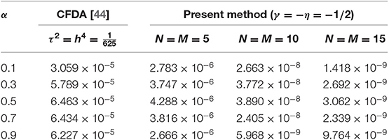
Table 1. Case I: The L^∞-error for Example 5.1.

TABLE 2

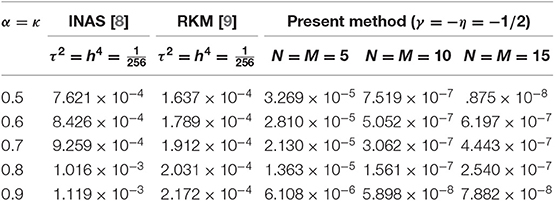
Table 2. Case II: The L^∞-error for example 5.1.

TABLE 3

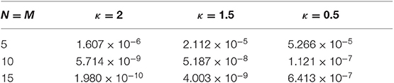
Table 3. Case III: The L^∞- errors for Example 5.1 vs. κ with γ = η = 0.

Example 5.2. Consider the following two-dimensional problem:

$\begin{array}{ll}\frac{\partial U(x,y,t)}{\partial t}=\left(1{+}_0{D}_t^{w(\nu )}\right)\left(\frac{{\partial }^{2}U(x,y,t)}{\partial x^2}+\frac{{\partial }^{2}U(x,y,t)}{\partial y^2}\right)& (53)\\ +H(x,y,t),\end{array}$

The initial condition, the boundary conditions and the right side function H are selected such as the continuous problem has an exact non-smooth solution in time direction U(x, y, t) = e^x+yt^α+1.

The space-time graphs of the absolute error functions with ω(ν) = Γ(1 + α + ν) at different values of t = 0.25, 0.5, 0.75, 1 with γ = −η = 1/2 and N = M = K = 8 are displayed in Figure 1. A comparison between the results obtained by the Jacobi–Galerkin method with the corresponding results obtained by the explicit numerical approximation scheme (ENAS) [45], the Implicit numerical approximation scheme (INAS) [45] and the compact finite difference approximation (CFDA) [10] are displayed in Tables 4, 5, respectively.

FIGURE 1

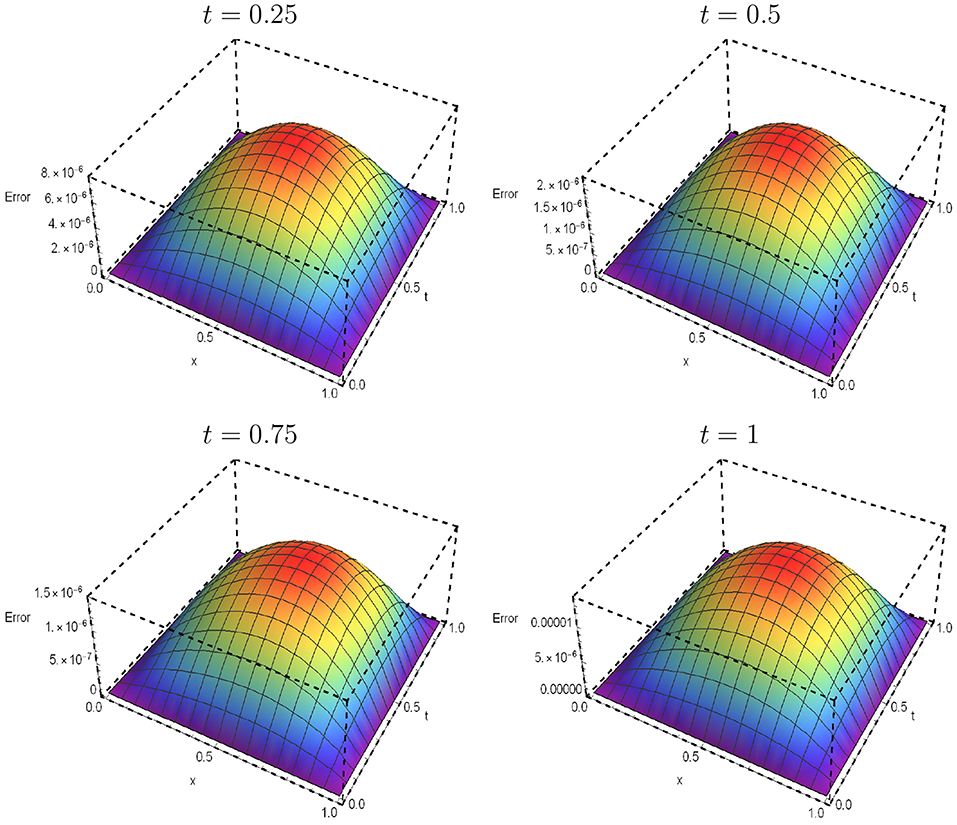
Figure 1. The space-time graphs of the absolute error functions for Example 0.0.2 at various choices of t with γ = −η = 1/2, N = M = K = 8 and ω(ν) = Γ(1+α+ν), α = 0.5.

TABLE 4

Table 4. The L^∞- errors for Example 5.2 with ω(ν) = δ(ν−1+α).

TABLE 5

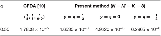
Table 5. The L^∞- errors for Example 5.2 with ω(ν) = δ(ν − 1 + α).

6. Conclusion

We have presented a Galerkin technique for solving the distributed-order time-fractional Rayleigh-Stokes problem for a generalized second-grade fluid with Jacobi polynomials that is efficient, adaptable to different operators, and easily generalizes to multiple dimensions. By expanding the model solution in terms of Jacobi polynomials in both time and space, we were able to derive adaptable schemes those easily accommodate the distributed fractional-order differential operator. All the calculations can be performed numerically with reasonable accuracy and with relatively small number of degrees of freedom. It should be pointed out that the proposed method to discretize the model equation could also accommodate other numerical methods. For instance, if the model solution is not smooth in time, the order of convergence of the spectral Galerkin schemes may be deteriorated. That could be prevented by simply replacing the Jacobi basis functions in time by fractional order Jacobi functions or using smoothing transformations and deriving the corresponding mass and diffusion matrices by following the same procedure as we described in this study.

Data Availability Statement

All datasets generated for this study are included in the article/supplementary material.

Author Contributions

All authors listed have made a substantial, direct and intellectual contribution to the work, and approved it for publication.

Conflict of Interest

The authors declare that the research was conducted in the absence of any commercial or financial relationships that could be construed as a potential conflict of interest.

References

1. Hafez RM, Zaky MA. High-order continuous Galerkin methods for multi-dimensional advection–reaction–diffusion problems. Eng Comput. (2019) 1–17. doi: 10.1007/s00366-019-00797-y

CrossRef Full Text | Google Scholar

2. Zhang X, Lv M, Crawford JW, Young IM. The impact of boundary on the fractional advection–dispersion equation for solute transport in soil: Defining the fractional dispersive flux with the Caputo derivatives. Adv Water Resour. (2007) 30:1205–17. doi: 10.1016/j.advwatres.2006.11.002

CrossRef Full Text | Google Scholar

3. Fetecau C, Jamil M, Fetecau C, Vieru D. The Rayleigh–Stokes problem for an edge in a generalized Oldroyd-B fluid. Z Angew Mathematik Physik. (2009) 60:921–33. doi: 10.1007/s00033-008-8055-5

CrossRef Full Text | Google Scholar

4. Shen F, Tan W, Zhao Y, Masuoka T. The Rayleigh–Stokes problem for a heated generalized second grade fluid with fractional derivative model. Nonlinear Anal Real World Appl. (2006) 7:1072–80. doi: 10.1016/j.nonrwa.2005.09.007

CrossRef Full Text | Google Scholar

5. Girault V, Saadouni M. On a time-dependent grade-two fluid model in two dimensions. Comput Math Appl. (2007) 53:347–60. doi: 10.1016/j.camwa.2006.02.048

CrossRef Full Text | Google Scholar

6. Zhao C, Yang C. Exact solutions for electro-osmotic flow of viscoelastic fluids in rectangular micro-channels. Appl Math Comput. (2009) 211:502–9. doi: 10.1016/j.amc.2009.01.068

CrossRef Full Text | Google Scholar

7. Xue C, Nie J. Exact solutions of the Rayleigh–Stokes problem for a heated generalized second grade fluid in a porous half-space. Appl Math Modell. (2009) 33:524–31. doi: 10.1016/j.apm.2007.11.015

CrossRef Full Text | Google Scholar

8. Wu C. Numerical solution for Stokes' first problem for a heated generalized second grade fluid with fractional derivative. Appl Num Math. (2009) 59:2571–83. doi: 10.1016/j.apnum.2009.05.009

CrossRef Full Text | Google Scholar

9. Lin Y, Jiang W. Numerical method for Stokes' first problem for a heated generalized second grade fluid with fractional derivative. Num Methods Partial Diff Equ. (2011) 27:1599–609. doi: 10.1002/num.20598

CrossRef Full Text | Google Scholar

10. Mohebbi A, Abbaszadeh M, Dehghan M. Compact finite difference scheme and RBF meshless approach for solving 2D Rayleigh–Stokes problem for a heated generalized second grade fluid with fractional derivatives. Comput Methods Appl Mech Eng. (2013) 264:163–77. doi: 10.1016/j.cma.2013.05.012

CrossRef Full Text | Google Scholar

11. Bazhlekova E, Jin B, Lazarov R, Zhou Z. An analysis of the Rayleigh–Stokes problem for a generalized second-grade fluid. Numerische Mathematik. (2015) 131:1–31. doi: 10.1007/s00211-014-0685-2

PubMed Abstract | CrossRef Full Text | Google Scholar

12. Abdelkawy MA, Alqahtani RT. Shifted Jacobi collocation method for solving multi-dimensional fractional Stokes' first problem for a heated generalized second grade fluid. Adv Diff Equ. (2016) 2016:114. doi: 10.1186/s13662-016-0845-z

CrossRef Full Text | Google Scholar

13. Bhrawy AH, Zaky MA, Alzaidy JF. Two shifted Jacobi-Gauss collocation schemes for solving two-dimensional variable-order fractional Rayleigh-Stokes problem. Adv Diff Equ. (2016) 2016:272. doi: 10.1186/s13662-016-0998-9

CrossRef Full Text | Google Scholar

14. Dehghan M, Abbaszadeh M. A finite element method for the numerical solution of Rayleigh–Stokes problem for a heated generalized second grade fluid with fractional derivatives. Eng Comput. (2017) 33:587–605. doi: 10.1007/s00366-016-0491-9

CrossRef Full Text | Google Scholar

15. Shivanian E, Jafarabadi A. Rayleigh–Stokes problem for a heated generalized second grade fluid with fractional derivatives: a stable scheme based on spectral meshless radial point interpolation. Eng Comput. (2018) 34:77–90. doi: 10.1007/s00366-017-0522-1

CrossRef Full Text | Google Scholar

16. Zaky MA. An improved tau method for the multi-dimensional fractional Rayleigh–Stokes problem for a heated generalized second grade fluid. Comput Math Appl. (2018) 75:2243–58. doi: 10.1016/j.camwa.2017.12.004

CrossRef Full Text | Google Scholar

17. Yang X, Jiang X. Numerical algorithm for two dimensional fractional Stokes' first problem for a heated generalized second grade fluid with smooth and non-smooth solution. Comput Math Appl. (2019) 78:1562–71. doi: 10.1016/j.camwa.2019.03.029

CrossRef Full Text | Google Scholar

18. Odibat Z, Baleanu D. A linearization-based approach of homotopy analysis method for non-linear time-fractional parabolic PDEs. Math Methods Appl Sci. (2019) 42:7222–32. doi: 10.1002/mma.5829

CrossRef Full Text | Google Scholar

19. Singh J, Kumar D, Baleanu D, Rathore S. On the local fractional wave equation in fractal strings. Math Methods Appl Sci. (2019) 42:1588–95. doi: 10.1002/mma.5458

CrossRef Full Text | Google Scholar

20. Kumar D, Singh J, Tanwar K, Baleanu D. A new fractional exothermic reactions model having constant heat source in porous media with power, exponential and Mittag-Leffler laws. Int J Heat Mass Transfer. (2019) 138:1222–7. doi: 10.1016/j.ijheatmasstransfer.2019.04.094

CrossRef Full Text | Google Scholar

21. Katsikadelis JT. Numerical solution of distributed order fractional differential equations. J Comput Phys. (2014) 259:11–22. doi: 10.1016/j.jcp.2013.11.013

CrossRef Full Text | Google Scholar

22. Mashayekhi S, Razzaghi M. Numerical solution of distributed order fractional differential equations by hybrid functions. J Comput Phys. (2016) 315:169–81. doi: 10.1016/j.jcp.2016.01.041

CrossRef Full Text | Google Scholar

23. Zaky M, Doha E, Machado JT. A spectral numerical method for solving distributed-order fractional initial value problems. J Comput Nonlinear Dyn. (2018) 13:101007. doi: 10.1115/1.4041030

CrossRef Full Text | Google Scholar

24. Morgado ML, Rebelo M. Numerical approximation of distributed order reaction–diffusion equations. J Comput Appl Math. (2015) 275:216–27. doi: 10.1016/j.cam.2014.07.029

CrossRef Full Text | Google Scholar

25. Abdelkawy M, Lopes AM, Zaky M. Shifted fractional Jacobi spectral algorithm for solving distributed order time-fractional reaction–diffusion equations. Comput Appl Math. (2019) 38:81. doi: 10.1007/s40314-019-0845-1

CrossRef Full Text | Google Scholar

26. Zaky MA, Machado JT. Multi-dimensional spectral tau methods for distributed-order fractional diffusion equations. Comput Appl Math. (2019) 79:476–88. doi: 10.1016/j.camwa.2019.07.008

CrossRef Full Text | Google Scholar

27. Abbaszadeh M. Error estimate of second-order finite difference scheme for solving the Riesz space distributed-order diffusion equation. Appl Math Lett. (2019) 88:179–85. doi: 10.1016/j.aml.2018.08.024

CrossRef Full Text | Google Scholar

28. Kazmi K, Khaliq AQ. An efficient split-step method for distributed-order space-fractional reaction-diffusion equations with time-dependent boundary conditions. Appl Num Math. (2019) 147:142–60. doi: 10.1016/j.apnum.2019.08.019

CrossRef Full Text | Google Scholar

29. Fan W, Liu F. A numerical method for solving the two-dimensional distributed order space-fractional diffusion equation on an irregular convex domain. Appl Math Lett. (2018) 77:114–21. doi: 10.1016/j.aml.2017.10.005

CrossRef Full Text | Google Scholar

30. Bhrawy A, Zaky M. Numerical simulation of multi-dimensional distributed-order generalized Schrödinger equations. Nonlinear Dyn. (2017) 89:1415–32. doi: 10.1007/s11071-017-3525-y

CrossRef Full Text | Google Scholar

31. Zaky M, Machado JT. On the formulation and numerical simulation of distributed-order fractional optimal control problems. Commun Nonlinear Sci Num Simul. (2017) 52:177–89. doi: 10.1016/j.cnsns.2017.04.026

CrossRef Full Text | Google Scholar

32. Zaky MA. A Legendre collocation method for distributed-order fractional optimal control problems. Nonlinear Dyn. (2018) 91:2667–81. doi: 10.1007/s11071-017-4038-4

CrossRef Full Text | Google Scholar

33. Zaky MA. Recovery of high order accuracy in Jacobi spectral collocation methods for fractional terminal value problems with non-smooth solutions. J Comput Appl Math. (2019) 357:103–22. doi: 10.1016/j.cam.2019.01.046

CrossRef Full Text | Google Scholar

34. Zaky MA, Ameen IG. On the rate of convergence of spectral collocation methods for nonlinear multi-order fractional initial value problems. Comput Appl Math. (2019) 38:144. doi: 10.1007/s40314-019-0922-5

CrossRef Full Text | Google Scholar

35. Zaky MA, Ameen IG. A priori error estimates of a Jacobi spectral method for nonlinear systems of fractional boundary value problems and related Volterra-Fredholm integral equations with smooth solutions. Num Algor. (2019). doi: 10.1007/s11075-019-00743-5. [Epub ahead of print].

CrossRef Full Text | Google Scholar

36. Doha E, Hafez R, Youssri Y. Shifted Jacobi spectral-Galerkin method for solving hyperbolic partial differential equations. Comput Math Appl. (2019) 78:889–904. doi: 10.1016/j.camwa.2019.03.011

CrossRef Full Text | Google Scholar

37. Bhrawy A, Doha EH, Baleanu D, Ezz-Eldien SS. A spectral tau algorithm based on Jacobi operational matrix for numerical solution of time fractional diffusion-wave equations. J Comput Phys. (2015) 293:142–56. doi: 10.1016/j.jcp.2014.03.039

CrossRef Full Text | Google Scholar

38. Alsuyuti MM, Doha EH, Ezz-Eldien SS, Bayoumi BI, Baleanu D. Modified Galerkin algorithm for solving multitype fractional differential equations. Math Methods Appl Sci. (2019) 42:1389–412. doi: 10.1002/mma.5431

CrossRef Full Text | Google Scholar

39. Huang LL, Liu BQ, Baleanu D, Wu GC. Numerical solutions of interval-valued fractional nonlinear differential equations. Eur Phys J Plus. (2019) 134:220. doi: 10.1140/epjp/i2019-12746-3

CrossRef Full Text | Google Scholar

40. Baleanu D, Shiri B, Srivastava H, Al Qurashi M. A Chebyshev spectral method based on operational matrix for fractional differential equations involving non-singular Mittag-Leffler kernel. Adv Diff Equ. (2018) 2018:353. doi: 10.1186/s13662-018-1822-5

CrossRef Full Text | Google Scholar

41. Baleanu D, Shiri B. Collocation methods for fractional differential equations involving non-singular kernel. Chaos Solitons Fractals. (2018) 116:136–45. doi: 10.1016/j.chaos.2018.09.020

CrossRef Full Text | Google Scholar

42. Doha E. On the construction of recurrence relations for the expansion and connection coefficients in series of Jacobi polynomials. J Phys A Math Gen. (2004) 37:657. doi: 10.1088/0305-4470/37/3/010

CrossRef Full Text | Google Scholar

43. Bhrawy A, Zaky MA. A method based on the Jacobi tau approximation for solving multi-term time–space fractional partial differential equations. J Comput Phys. (2015) 281:876–95. doi: 10.1016/j.jcp.2014.10.060

CrossRef Full Text | Google Scholar

44. Chen Y, Chen CM. Numerical algorithm for solving the Stokes' first problem for a heated generalized second grade fluid with fractional derivative. Num Algor. (2018) 77:939–53. doi: 10.1007/s11075-017-0348-3

CrossRef Full Text | Google Scholar

45. Chen CM, Liu F, Anh V. Numerical analysis of the Rayleigh–Stokes problem for a heated generalized second grade fluid with fractional derivatives. Appl Math Comput. (2008) 204:340–51. doi: 10.1016/j.amc.2008.06.052

CrossRef Full Text | Google Scholar