Physics-Informed Neural Networks for Cardiac Activation Mapping

1. Introduction

Atrial fibrillation is the most common arrhythmia in the heart, affecting between 2.7 and 6.1 million people in the United States alone [1]. A standard procedure to diagnose and treat atrial fibrillation is the acquisition of electrical activation maps, where a catheter is inserted to the cardiac chamber and the electrode at the tip records the activation time of the tissue at a given location. This process is repeated at multiple sites to cover the entire atrium. Finally, these measurements are interpolated to create a complete electro-anatomic map of the chamber [2]. The most common approach to interpolate the data is to use linear functions [2, 3] or radial basis functions [4]. There is a recent focus into incorporating the uncertainty associated with these maps [3, 5]. This is relevant since there are multiple sources of noise that can pollute the activation map, such as the position of the electrode and the difficulty to determine the activation time from an electrical signal. There is also uncertainty in the interpolation method that is used, which can be relevant particularly in regions of low data density. However, most current techniques [2, 3] ignore the underlying physics of the electrical wave propagation [6]. This can result in unrealistic interpolations with artificially high conduction velocities. The strategies that do include the physics assume either a constant conduction velocity field [7] or a fixed amount of activation sources [8]. Additionally, there are no recommendations on the best strategy to acquire new measurements toward reducing the procedure time and improving its accuracy.

Deep learning has revolutionized many fields in engineering and medical sciences. However, in the context of activation mapping, we have to rely on a few sparse activation measurements. To address the limitations of deep learning associated with sparse data, recent techniques have emerged to incorporate the underlying physics, as governed by partial differential equations, into neural networks [9–13]. This powerful framework allows to train a neural network that simultaneously approximates the data and conforms to the partial differential equations that represents the physical knowledge of the system [14], a concept known as physics-informed neural networks.

Here, we propose to use a physics-informed neural network to create activation maps of the atria [15], more accurately and efficiently than with linear interpolation alone. We incorporate the physical knowledge using the Eikonal equation, which describes the behavior of the activation times for a conduction velocity field. We estimate the uncertainty in our predictions using randomized prior functions [16]. In addition, we take advantage of these estimates to create an active learning algorithm that, for a given set of initial measurements, recommends the location of the next measurement to systematically reduce the model error [17]. We highlight the advantages of this method for both a two-dimensional benchmark problem and a three-dimensional personalized geometry of the left atrium.

This manuscript is organized as follows: In section 2 we introduce the physics-informed neural network, the method to estimate uncertainties and the active learning algorithm. In section 3, we show two numerical experiments to test the accuracy of the method. We end this manuscript with a discussion and future directions in section 4.

2. Methods

In this section we introduce a physics-informed neural network [9, 18] to interpolate activation times for cardiac electrophysiology. We also present the methodology to estimate uncertainties and an active learning algorithm to efficiently sample the data acquisition space.

2.1. Physics Informed Neural Network for Activation Times

The electrical activation map of the heart can be related to a traveling wave, where the wavefront represents the location of cells that are depolarizing [19]. The time at which cells depolarize is referred to as the activation time and corresponds to an increase in transmembrane potential above a certain threshold and the initiation of the cell contraction. The activation times of the traveling wave must satisfy the Eikonal equation:

$\begin{array}{ll}\Vert \nabla T(\text{x})\Vert =\frac{1}{V(\text{x})}& (1)\end{array}$

where $T(\text{x})$ is the activation time at a point $\text{x}$ and $V(\text{x})$ represents the local speed of the wave at the same location, which is referred to as the conduction velocity. We can rewrite (1) in residual form as

$\begin{array}{ll}R(\text{x}):=V(\text{x})\Vert \nabla T\Vert -1=0.& (2)\end{array}$

Further, we approximate both the activation time $T(\text{x})$ and conduction velocity $V(\text{x})$ by

$\begin{array}{ll}T(\text{x})\approx N{N}_T(\text{x},{\text{θ}}_T),& (3)\end{array}$

$\begin{array}{ll}V(\text{x})\approx N{N}_V(\text{x},{\text{θ}}_V),& (4)\end{array}$

where NN_T and NN_V are neural networks with parameters ${\text{θ}}_T$ and ${\text{θ}}_V$, respectively, that need to be trained in order to obtain a good approximation. Since the conduction velocity is strictly positive and is bounded in a physiological range, we pass the output of the last layer through a sigmoid function σ so that the conduction velocity neural network reads

$\begin{array}{ll}V(\text{x})=V_{max}·\sigma (N{N}_V(\text{x})),& (5)\end{array}$

where V_max represents the maximum conduction velocity, specified by the user. Finally, we define a loss function to train our model:

$\begin{array}{l}{L}({\text{θ}}_T,{\text{θ}}_V)=\frac{1}{N_T}{\displaystyle \sum _{i=1}^{N_T}}{(T({\text{x}}_i)-{\widehat{T}}_i)}^2+\frac{1}{N_R}{\displaystyle \sum _{i=1}^{N_R}}R{({\text{x}}_i)}^2\\ +{\alpha }_{TV}\frac{1}{N_R}{\displaystyle \sum _{i=1}^{N_R}}\Vert \nabla V({\text{x}}_i)\Vert +{\alpha }_{L2}{\displaystyle \sum _{i=1}^{N_{{\theta }_T}}}{{\theta }_{Ti}}^2.& (6)\end{array}$

Figure 1 illustrates the first two terms of the loss function: The first term enforces that the output of neural network coincides with the N_T activation time measurements available ${\widehat{T}}_i$, the second term enforces that the output of networks satisfies the Eikonal equation at N_R collocation points. The third and fourth terms serve as regularization for the inverse problem. The third term, which we evaluate at the N_R collocation points, is a total variation regularization for the conduction velocity, which allows discrete jumps in the solution. We select this term to model slow regions of conduction, such as fibrotic patches. Finally, we use L₂ regularization on the weights of the activation time neural network, for reasons we explain in the following section. We solve the following minimization problem to train the neural networks and find the optimal parameters:

$\begin{array}{ll}{\displaystyle \underset{({\text{θ}}_T,{\text{θ}}_V)}{arg min}}{L}({\text{θ}}_T,{\text{θ}}_V)& (7)\end{array}$

FIGURE 1

Figure 1. Physics-informed neural networks for activation mapping. We use two neural networks to approximate the activation time T and the conduction velocity V. We train the networks with a loss function that accounts for the similarity between the output of the network and the data, the physics of the problem using the Eikonal equation, and the regularization terms.

2.2. Uncertainty Quantification

We will be interested in quantifying the uncertainty in our predictions to both inform physicians about the quality of the estimates as well as to use active learning techniques to judiciously acquire new measurements. Given the large number of parameters in neural networks, using gold-standard methods for Bayesian inference, such as Markov Chain Monte Carlo, is prohibitively expensive. Instead, we borrow ideas from deep reinforcement learning and use randomized prior functions [16] to quantify the epistemic/model uncertainty associated with our neural network predictions. The key idea is to introduce an additional neural network with the same architecture, such that:

$\begin{array}{ll}T(\text{x})\approx N{N}_T(\text{x},{\text{θ}}_T)+N{N}_T(\text{x},{\widetilde{\text{θ}}}_T)& (8)\end{array}$

$\begin{array}{ll}V(\text{x})\approx N{N}_V(\text{x},{\text{θ}}_V)+N{N}_V(\text{x},{\widetilde{\text{θ}}}_V)& (9)\end{array}$

We draw the parameters ${\widetilde{\text{θ}}}_T,{\widetilde{\text{θ}}}_V$ from a prior distribution and keep them fixed during the training process. In this approach, a mean squared loss is equivalent to a normal likelihood for the data and the L2 regularization is equivalent to a zero mean normal prior for the neural network parameters. It can be shown that training the parameters to minimize the loss is equivalent to generating samples from a posterior distribution $p(\text{θ}|{D})$ when using a linear regressor [16]. To account for uncertainty in our predictions, we use an ensemble of neural networks initialized with different prior functions defined by the parameters ${\widetilde{\text{θ}}}_T,{\widetilde{\text{θ}}}_V$, which we randomly sample with Glorot initialization [20]. Additionally, we perturb our data with Gaussian noise with variance ${\sigma }_N^2$ to train each network of the ensemble with a slightly different dataset. Our final prediction is obtained as the mean output of the ensemble of neural networks.

2.3. Active Learning

We take advantage of the uncertainty estimates described in the previous section to create an adaptive sampling strategy. We start with a small number of randomly located samples, fit our model, and then acquire the next measurement at the point that we estimate to reduce the predictive model error the most. We iteratively fit the model and acquire samples until we reach a user-defined convergence or until we exceed our budget or time to acquire new data. Since the exact predictive error is unknown, there are several heuristics to determine where to place the next sample. A common approach is to select the location where the uncertainty is the highest, which we can quantify by evaluating the entropy of the posterior distribution $p(T|{D})$ [21]. We can view the entropy as negative information and, in the case of a Gaussian posterior, it is proportional to the variance, which has also been proposed for active learning [22]. In our computational experiments, we observe that the predictive posterior distribution $p(T|{D})$ is generally not Gaussian and we opt to use a non-parametric estimator for the entropy [23, 24]. This is likely induced by the discrete jumps in conduction velocity that are a result of the total variation regularization term. Algorithm 1 summarizes the procedure. Since the initial predictions will be inaccurate due to the lack of data, it is not necessary to train the neural network completely to obtain the uncertainty estimates and start the active learning process. We can train the model and acquire data in parallel, as the prediction step and the entropy computation are of negligible computational cost. Here, we iteratively refine the predictions and the uncertainty estimates as more data become available and the model is trained.

ALGORITHM 1

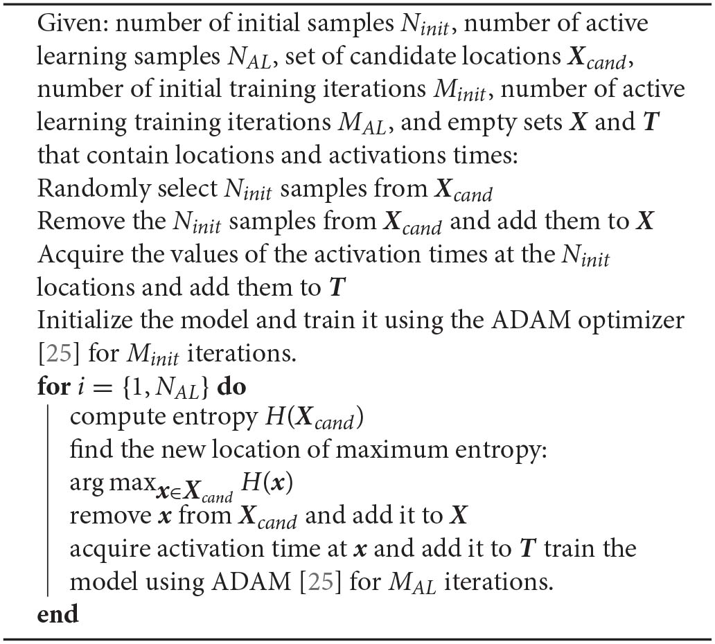
Algorithm 1. Active learning algorithm to iteratively identify the most efficient sampling points

2.4. Application to Surfaces From Electro-Anatomic Mapping

During electro-anatomic mapping, data can only be acquired on the cardiac surface, either of the ventricles or the atria. We thus represent the resulting map as a surface in three dimensions and neglect the thickness of the atrial wall. This is a reasonable assumption since the thickness-to-diameter ratio of the atria is in the order of 0.05. Our assumption implies that the electrical wave can only travel along the surface and not perpendicular to it. To account for this constraint, we include an additional loss term:

$\begin{array}{ll}{{L}}_N={\alpha }_N\frac{1}{N_R}{\displaystyle \sum _{i=1}^{N_R}}{(\nabla T\left({\text{x}}_i\right)·{\text{N}}_i)}^2& (10)\end{array}$

This form favors solutions where the activation time gradients are orthogonal to the surface normal ${\text{N}}_i$. To implement this constraint, we assume a triangular discretization of either the left or right atrium, which we obtain from magnetic resonance imaging or computed-tomography imaging. We can then compute a surface normal ${\text{N}}_i$ for each triangle. We define the N_R collocation points as the centroids of each triangle in the mesh ${\text{x}}_i$. We enforce this constraint weakly by adding a factor α_N. If the gradient of the activation times were exactly orthogonal to the triangle normals, it would force a linear interpolation between mesh nodes in the neural network, which is not desirable and unlikely attainable.

2.5. Implementation and Training

We implement all models in Tensorflow [26] and use the Tensorflow ADAM optimizer [25] with default parameters and a learning rate of 0.001. For the N_R collocation points, we use a minibatch implementation, in which we use a subset of all available collocation points to compute the loss function and its gradient. For the two-dimensional benchmark problem, we randomly sample N_mb points using a Latin hypercube design [27] and use them as collocation points. For the three-dimensional left atrium, we shuffle the order of the triangles in the mesh and divide them into batches of size N_mb. For each iteration, we use the centroid locations of the triangles of one of these batches as collocation points and loop through them as the optimization progresses.

3. Numerical Experiments

In this section, we explore our method using a two-dimensional benchmark problem and a three-dimensional personalized left atrium. We also quantify the effectiveness of the active learning algorithm.

3.1. Benchmark Problem

To characterize the performance of the proposed model, we design a synthetic benchmark problem that analytically satisfies the Eikonal equation. We introduce a discontinuity in the conduction velocity and collision of two wavefronts in the following form:

$\begin{array}{ll}T\left(x,y\right)=min\left(\sqrt{x^2+y^2},0.7\sqrt{{\left(x-1\right)}^2+{\left(y-1\right)}^2}\right)& (11)\end{array}$

$\begin{array}{ll}V\left(x,y\right)=\{\begin{array}{c}1.0\text{ if}\sqrt{x^2+y^2}<0.7\sqrt{{\left(x-1\right)}^2+{\left(y-1\right)}^2}\hfill \\ \frac{1.0}{0.7}\text{ otherwise}\hfill \end{array}& (12)\end{array}$

with x, y ∈ [0, 1]. Figure 2, left, illustrates the exact mapping of the activation times and conduction velocity. We generate N = 50 samples with a Latin hypercube design and train our model. We only have data on the activation times and we predict both the activation times and the conduction velocity. We use 5 hidden layers with 20 neurons each for the activation time neural network and 5 hidden layers with 5 neurons each for conduction velocity neural network. We perform a sensitivity study for α_TV and α_L2 and then select them to ${\alpha }_{TV}=10^{-7}$ and ${\alpha }_{L2}=10^{-9}$ while keeping all other parameters fixed. We train the network for 50,000 ADAM iterations with a batch size N_mb = 100 and then train with the L-BFGS method [28].

FIGURE 2

Figure 2. Benchmark problem activation times and conduction velocities. The top row shows the activation times, the bottom row the conduction velocity. The columns display the exact solution and the results of the physics-informed neural network (PINN), a neural network without physics, the Gaussian process regression, and the linear interpolation. The black circles indicate the sampling locations.

We compare our method against three other methodologies: a neural network with the same architecture and parameters except without including the physics, linear interpolation [2], and Gaussian process regression [3, 29]. In the neural network without physics, we compute the conduction velocity analytically as V = 1/||∇T||. In the linear interpolation case, we use the scatteredInterpolant function from MATLAB with linear extrapolation [2]. We compute the conduction velocity by approximating the gradient of the activation time with finite differences on a regular grid across the domain. Then, we calculate the conduction velocity as V = 1/||∇T||. For the Gaussian process regression, we use our open-source implementation [30] with a squared exponential kernel and automatic relevance determination. We compute the gradient of the resulting Gaussian process analytically and we use this value to compute the conduction velocity. We use the root mean squared error (RMSE) for the activation times and the mean absolute error (MAE) for the conduction velocity. We make this distinction to avoid the artificially high errors that will be reported in the root mean squared error near the discontinuity of conduction velocity.

Figures 2, 3 and Table 1 compare the results of the different methods against the exact solution. Qualitatively and quantitatively, the physics-informed neural network presents the best results for activation times and conduction velocity. It captures the wavefront collision and detects the two distinct regions of conduction velocity. The discontinuity in the conduction velocity is smoother in this method than in the data. Nonetheless, the neural networks outperform other methods, which show problematic representations of the conduction velocity. Since the neural network without physics and the Gaussian process regression are smooth, they are not capable of reproducing the discontinuity in the gradient that occurs when two wavefronts collide. This inevitably results in a region of zero activation time gradient, which results in an infinite conduction velocity. The linear interpolation suffers from a similar problem, although it will depend heavily in the location of the data. Figure 3 illustrates the numerical artifacts of these two methods compared to the Gaussian process regression by means of the solution along the x = y line.

FIGURE 3

Figure 3. Benchmark problem x = y line. The dashed lines show the exact analytical solution, the solid lines the different interpolation methods. The physics-informed neural network (PINN) captures the gradient of the activation times produced by the collision of two wavefronts and closely predicts the conduction velocity. The neural network and Gaussian process regression produce a smooth interpolation that generates oscillating conduction velocities, especially near the collision of the two wavefronts. The linear interpolation produces an approximation that is highly sensitive to the position of the data points.

TABLE 1

Table 1. Normalized errors for benchmark problem.

To conclude, we evaluate the performance of all four methods to noise. We introduce Gaussian noise with a standard deviation of 1, 5, and 10% of the maximum value of activation time and run all methods 30 times with the same datasets. In this case, we train the physics-informed neural network and the regular neural network for 100,000 ADAM iterations. Table 1 summarizes the results. We can see that the physics-informed neural network outperforms other methods except for the 5% noise case in the activation times. For the conduction velocity, the physics informed neural network performs better in all cases by a large margin. Gaussian process regression is as robust to noise as our approach, with similar levels of error for the activation times. Remarkably, the adding physics to the neural network reduces the error in both activation time and conduction velocity.

3.2. Uncertainty Quantification

To study the accuracy of our uncertainty estimates, we vary the number of neural networks trained in our randomized priors ensemble. We set the noise parameter to σ_N = 0.01, based on reported uncertainties [3]. We compute the entropy of a case with 30 samples from a Latin hypercube design and 5, 10, 30, 50, and 100 neural networks. We train the networks for 50,000 ADAM iterations with a mini-batch size of N_mb = 96. We define the entropy estimated by 100 neural networks as our ground truth and compute the root mean square error for the remaining cases. We also compute the time it takes to train the networks. Figure 4 summarizes the results of this study. We observe a trade-off between accuracy and cost: The error reduction rate is reduced when more than 30 neural networks are used; however, we observe a linear trend in the time it takes to train multiple networks. Yet, the time it takes to train 100 networks is only four times of what it takes to train a single network. The baseline wall clock time to train one work was 404 s using a laptop with 8 CPUs. Combining these observations, we set the number of neural networks to estimate the uncertainty to 30.

FIGURE 4

Figure 4. Uncertainty quantification and effect of number of neural networks. Entropy predicted by 10, 30, and 100 neural networks, and the tradeoff between entropy reduction and normalized training time for increasing number of neural networks. The black circles indicate the sampling locations.

We also test the hypothesis that the maximum entropy is co-localized with the predictive error of the model. If this is true, the active learning approach will be effective, since placing a new sample at the point of maximum entropy will reduce the error. We run the two-dimensional example with the same parameters specified in the previous sections with 30 samples drawn from a Latin hypercube design and train 30 neural networks in parallel. Figure 5 reveals that regions of high entropy are co-located with regions of high error and that the point of maximum entropy is close to the point of maximum error.

FIGURE 5

Figure 5. Correlation of uncertainty and error. For the benchmark problem, trained with 30 samples, the computed entropy tends to be higher at regions where the error is higher and the points of maximum entropy and maximum error (⋆) are co-located. The black circles indicate the sampling locations.

3.3. Active Learning

To test the effectiveness of the proposed active learning method, we train models with 30 different initial conditions. We start with N_init = 10 samples and follow algorithm 1, acquiring N_AL = 40 additional samples. We also train 30 models where N samples are placed using a Latin hypercube design for N = {20, 30, 40, 50}. Figure 6 summarizes the performance of our active learning algorithm. We observe that the active learning strategy quickly reduces the error until a total of 20 samples are obtained. Then, the error reduction is slower and reaches an asymptote. However, when we compare it to the Latin hypercube design, we see that the error is smaller in all cases. We test this hypothesis with the Mann-Whithney test [31] and obtain a significant difference for all cases, both in activation time (p < 10⁻⁷) and in conduction velocity (p < 0.015). The error in the conduction velocity is higher than for the activation time in all cases. This difference may be explained by the difficulty in capturing the discontinuity of the conduction velocity set in the example. A small difference in where the different conduction velocity regions are identified can cause a large error.

FIGURE 6

Figure 6. Benchmark problem and active learning. We perform 30 simulations of active learning with different initial samples and compare them against a Latin hypercube design. In the middle and right box plots, we observe a significant reduction in activation time normalized root mean squared error (p < 10⁻⁷) and in conduction velocity normalized mean absolute error (p < 0.015) when using the active learning algorithm.

3.4. Left Atrium

To test our model in three dimensions, we studying the electrophysiology of the left atrium. We obtain the mesh from one of the examples of the MICCAI challenge dataset [32] created from magnetic resonance imaging. We use the monodomain model for the tissue and the Fenton Karma model for cells under the MLR1 conditions [33]. We use the open-source software cbcbeat [34] to perform the simulation. We consider two cases, one where the conductivity is homogeneous at 0.1 mm²/ms in the entire domain and one where it is heterogeneous such that half of the domain has a reduced conductivity of 0.05 mm²/ms. In both cases, we initiate the activation at the center of the septum. We define the activation time as the time at which the transmembrane potential reaches 0 mV. We then compute the conduction velocity as V = 1/||∇ T|, and approximate the gradient of the activation time with a finite-element approximation constructed based on the triangular mesh. For the neural network, we use the same parameters as before, except that we now use seven layers of 20 neurons for the activation time network and a maximum conduction velocity of V_max = 1 m/s. We consider two experiments.

In the first experiment, we set the number of samples by the optimal density [2], which corresponds to 1.05 samples/cm². We randomly choose nodes in the mesh and use the activation times as data points. We repeat this process 30 times and compare the error to using a linear interpolation trained with the same data as detailed in section 3.1 with a Wilcoxon test [35]. Figure 7, left, shows that the error for the physics-informed neural network is significantly lower than for the linear interpolation (p < 10⁻⁵) for both the homogeneous constant conductivity case (median 1.53, range 1.34–1.85 ms vs. median 3.92, range 3.42–5.34 ms) and the heterogeneous case with reduced conductivity in half of the domain (median 2.23, range 1.84–2.84 ms vs. median 4.77, range 3.90-6.02 ms).

FIGURE 7

Figure 7. Left atrium accuracy in activation times and conduction velocities. Performance of the physics-neural network (PINN) vs. linear interpolation, top left. The physics-neural network significantly reduces the root mean squared error (RMSE) in the homogeneous case with constant conductivity and in the heterogeneous case where the conductivity was reduced in half of the domain (p < 10⁻⁵). Performance of the active learning algorithm for these two cases, top center and top right. Active learning decreases the root mean squared error of the activation times and the mean absolute error of the conduction velocity. The dashed line represents the median error achieved by linear interpolation at optimal sample density. Sample density required by the active learning approach to achieve the median error of the linear interpolation method at optimal sample density, bottom left. Comparison of active learning against random selection in the case of constant conductivity (bottom center) and reduced conductivity (bottom right). The active learning algorithm significantly reduces the error in all cases (p < 0.002).

In the second experiment, we explore the performance of the active learning algorithm by running 30 cases that start with N_init = 10 randomly selected samples, which corresponds to a density of 0.081 samples/cm². We acquire samples until we reach 90 measurements, which corresponds to a density of 0.734 samples/cm². Figure 7 shows the accuracy of the method and Figures 8, 9 illustrate the evolution of the active learning algorithm. We observe that in both cases, homogeneous conductivity and reduced conductivity in half of the domain, the active learning algorithm reduces the error and converges to the same value, irrespective of the initial conditions. This is reflected in the small range of errors in activation times at 0.73 samples/cm² for the homogeneous case (1.01–1.88 ms) and the heterogeneous case (1.38–2.28 ms). The mean absolute errors in conduction velocity are relatively high for both cases (constant: median 0.086, range 0.083–0.101 m/s; half: median 0.085, range 0.081–0.095 ms). This can be explained, at least in part, by the difficulty of computing conduction velocities from the cardiac electrophysiology simulation. As Figures 8, 9 show, there are regions of artificially high conduction velocities, especially when two wavefronts collide, which may bias the reported error. Nonetheless, the method can delineate the two regions of conduction velocity in the heterogeneous case, as Figure 9 confirms. We also compute the density required by the active learning algorithm to achieve the same median error in activation time as the linear interpolation at the optimal density of 1.05 samples/cm². This results in 3.92 ms in the constant conductivity case and 4.77 ms in the reduced conductivity case. The results show that a density of median 0.20, range 0.18–0.26 samples/cm² is needed for the homogeneous case and a density of median 0.24, range 0.16–0.30 samples/cm² for the heterogeneous case. Finally, we compare the performance of the active learning algorithm against randomly choosing samples by running 30 cases at 0.25 and 0.74 samples/cm². Figure 7, bottom center and right panels, shows that the active learning algorithm significantly reduces the error in activation times (p <0.002).

FIGURE 8

Figure 8. Evolution of active learning for the homogeneous case with constant conductivity. The top two rows show the activation times for different sample densities and the ground truth for two different views. The bottom rows represent the conduction velocity.

FIGURE 9

Figure 9. Evolution of active learning for the heterogeneous case with partly reduced conductivity. The top two rows show the activation times for different sample densities and the ground truth for two different views. The bottom rows represent the conduction velocity.

4. Discussion

In this work, we present a novel framework to create activation maps in cardiac electrophysiology by incorporating prior physical knowledge of the underlying wave propagation. To this end, we employ neural networks to represent the spatial distribution of activation times and conduction velocity, subject to physics-informed regularization prescribed by the Eikonal equation. In particular, we show that our method is able to capture the collision of wavefronts, a situation that is not captured by other state-of-the-art methods. This is a critical step toward reliably estimating conduction velocities and avoiding artificially high conduction velocity values. Our methodology directly predicts conduction velocities, without the need of creating ad-hoc techniques [36]. Further, it allows us to quantify the uncertainty in our predictions via randomized prior functions, which represents a useful tool in the clinical setting [3]. Notably, this uncertainty quantification comes at small computational cost, where we can train 30 networks in parallel, increasing the training time by only 1.75 × the time needed to train one network. The uncertainty estimates become the cornerstone of our active learning algorithm, which reduces the predictive error in both two- and three-dimensional cases. With this algorithm, we need fewer samples to achieve the same accuracy than that required in random allocation. This implies that the procedure of activation time sampling can be significantly reduced. In other words, for the same procedure time, the clinician can obtain more accurate estimates of the activation times and conduction velocity. In the way we designed the active learning algorithm, we can simultaneously train the neural networks and predict points for active learning, which makes the real time application of this methodology feasible in a clinical setting. In our experiments, we observed that 1 min of training per sample in a laptop with 8 cores was more than enough to obtain accurate results. In the future, we could easily accelerate this process by using graphic processing units or other dedicated hardware to train neural networks. If this is still not sufficient and samples can arrive faster than the training speed, we could extend the algorithm to make multiple recommendations for sample locations or simply gather more samples randomly in the vicinity of the current recommendation. Even though our method is computationally more expensive than other alternatives, the gains in accuracy could lead to reduction in procedural times for the patient, which outweighs the cost of training the model. Our methodology displays remarkable consistency and robustness and achieving similar error levels, irrespective of the initial set of samples.

Even though our method shows promising results when compared to existing solutions, it displays some limitations. First, we have ignored the anisotropy in conduction of cardiac tissue [19, 37]. However, we could easily use the anisotropic Eikonal equation in our loss and estimate fiber and cross-fiber conduction velocities. This would require information of the fiber orientations in the atria and ventricles. There are several methodologies to incorporate this information with ruled-based approaches [38, 39] and mapping techniques [40, 41]. On the estimation of uncertainties, we see two limitations: First, we have not included the noise that is generated by the acquisition of the activation times with the electrode. We can incorporate this source of uncertainty by estimating some variance in the activation times [3] and include it in the Gaussian perturbation σ_N that we use in the randomized prior functions. Second, our uncertainty estimates are only approximations, since the true uncertainties depend on the geodesic distance between points on the manifold and not on the Euclidean distance in ${{R}}^3$, which we have used to parametrize this problem [3, 42]. We can address this limitation by using more complex architectures, such as convolutional neural networks on graphs [43], which we plan to explore in the future. However, empirically, we see that active learning works well with this approximation. Finally, we have only tested our method with synthetic data and additional challenges could arise when applying it to real clinical data. We expect that the method will perform well for focal activations and macro re-entry tachycardia [2]. For localized re-entry or fibrillation, however, we expect that the method will not work, as the conduction velocity of the spiral wave depends on both time and space and the Eikonal equation does not hold. As a next step, we plan to test this methodology in a cohort of patients with focal activations or macro re-entry tachycardia [15].

In summary, we have presented a new and efficient methodology to acquire and create activation maps in cardiac electrophysiology. We believe that our approach will enable faster and more accurate acquisitions that will benefit the diagnosis of patients with cardiac arrhythmias.

Data Availability Statement

The datasets generated for this study are available on request to the corresponding author. Source code is available at https://github.com/fsahli/EikonalNet.

Author Contributions

FS, PP, DH, and EK designed the research and wrote the manuscript. FS, PP, and YY wrote the code and performed the simulations. FS and PP analyzed the data.

Funding

This work was supported by the School of Engineering Postdoctoral Fellowship from Pontificia Universidad Católica de Chile, the FONDECYT-Postdoctorado 3190355 awarded to FS, the US Department of Energy under the Advanced Scientific Computing Research grant DE-SC0019116 and the Defense Advanced Research Projects Agency grant HR00111890034 awarded PP. This publication has received funding from Millenium Science Initiative of the Ministry of Economy, Development and Tourism of Chile, grant Nucleus for Cardiovascular Magnetic Resonance.

Conflict of Interest

The authors declare that the research was conducted in the absence of any commercial or financial relationships that could be construed as a potential conflict of interest.

References

1. Benjamin EJ, Virani SS, Callaway CW, Chamberlain AM, Chang AR, Cheng S, et al. Heart disease and stroke statistics-2018 update: a report from the American Heart Association. Circulation. (2018) 137:e67. doi: 10.1161/CIR.0000000000000573

PubMed Abstract | CrossRef Full Text | Google Scholar

2. Williams SE, Harrison JL, Chubb H, Whitaker J, Kiedrowicz R, Rinaldi CA, et al. Local activation time sampling density for atrial tachycardia contact mapping: how much is enough? Europace. (2018) 20:e11–20. doi: 10.1093/europace/eux037

PubMed Abstract | CrossRef Full Text | Google Scholar

3. Coveney S, Corrado C, Roney C, Wilkinson R, Oakley J, Lindgren F, et al. Probabilistic interpolation of uncertain local activation times on human atrial manifolds. IEEE Trans Biomed Eng. (2019) 67:99–109. doi: 10.1109/TBME.2019.2908486

PubMed Abstract | CrossRef Full Text | Google Scholar

4. Masé M, Ravelli F. Automatic reconstruction of activation and velocity maps from electro-anatomic data by radial basis functions. In: 2010 Annual International Conference of the IEEE Engineering in Medicine and Biology. Buenos Aires: IEEE (2010). p. 2608–11. doi: 10.1109/IEMBS.2010.5626616

PubMed Abstract | CrossRef Full Text | Google Scholar

5. Quaglino A, Pezzuto S, Koutsourelakis P, Auricchio A, Krause R. Fast uncertainty quantification of activation sequences in patient-specific cardiac electrophysiology meeting clinical time constraints. Int J Numer Methods Biomed Eng. (2018) 34:e2985. doi: 10.1002/cnm.2985

PubMed Abstract | CrossRef Full Text | Google Scholar

6. Sahli Costabal F, Concha FA, Hurtado DE, Kuhl E. The importance of mechano-electrical feedback and inertia in cardiac electromechanics. Comput Methods Appl Mech Eng. (2017) 320:352–68. doi: 10.1016/j.cma.2017.03.015

CrossRef Full Text | Google Scholar

7. Jacquemet V. An eikonal-diffusion solver and its application to the interpolation and the simulation of reentrant cardiac activations. Comput Methods Prog Biomed. (2012) 108:548–58. doi: 10.1016/j.cmpb.2011.05.003

PubMed Abstract | CrossRef Full Text | Google Scholar

8. Kunisch K, Neic A, Plank G, Trautmann P. Inverse localization of earliest cardiac activation sites from activation maps based on the viscous Eikonal equation. J Math Biol. (2019) 79:2033–68. doi: 10.1007/s00285-019-01419-3

PubMed Abstract | CrossRef Full Text | Google Scholar

9. Raissi M, Perdikaris P, Karniadakis GE. Physics-informed neural networks: a deep learning framework for solving forward and inverse problems involving nonlinear partial differential equations. J Comput Phys. (2019) 378:686–707. doi: 10.1016/j.jcp.2018.10.045

CrossRef Full Text | Google Scholar

10. Yang Y, Perdikaris P. Adversarial uncertainty quantification in physics-informed neural networks. J Comput Phys. (2019) 394:136–52. doi: 10.1016/j.jcp.2019.05.027

CrossRef Full Text | Google Scholar

11. Zhu Y, Zabaras N, Koutsourelakis PS, Perdikaris P. Physics-constrained deep learning for high-dimensional surrogate modeling and uncertainty quantification without labeled data. J Comput Phys. (2019) 394:56–81. doi: 10.1016/j.jcp.2019.05.024

CrossRef Full Text | Google Scholar

12. Yang Y, Perdikaris P. Physics-informed deep generative models. arxiv [Preprint] arXiv:181203511. (2018).

Google Scholar

13. Tartakovsky AM, Marrero CO, Tartakovsky D, Barajas-Solano D. Learning parameters and constitutive relationships with physics informed deep neural networks. arxiv [Preprint] arXiv:180803398. (2018).

Google Scholar

14. Alber M, Buganza Tepole A, Cannon W, De S, Dura-Bernal S, Garikipati K, et al. Integrating machine learning and multiscale modeling: perspectives, challenges, and opportunities in the biological, biomedical, and behavioral sciences. npj Digit Med. (2019) 2:115. doi: 10.1038/s41746-019-0193-y

PubMed Abstract | CrossRef Full Text | Google Scholar

15. Sahli Costabal F, Zaman JAB, Kuhl E, Narayan SM. Interpreting activation mapping of atrial fibrillation: a hybrid computational/physiological study. Ann Biomed Eng. (2018) 46:257–69. doi: 10.1007/s10439-017-1969-3

PubMed Abstract | CrossRef Full Text | Google Scholar

16. Osband I, Aslanides J, Cassirer A. Randomized prior functions for deep reinforcement learning. In: Advances in Neural Information Processing Systems. Montreal, QC (2018). p. 8617–29.

Google Scholar

17. Costabal FS, Perdikaris P, Kuhl E, Hurtado DE. Multi-fidelity classification using Gaussian processes: accelerating the prediction of large-scale computational models. Comput Methods Appl Mech Eng. (2019) 357:112602. doi: 10.1016/j.cma.2019.112602

CrossRef Full Text | Google Scholar

18. Lagaris IE, Likas A, Fotiadis DI. Artificial neural networks for solving ordinary and partial differential equations. IEEE Trans Neural Netw. (1998) 9:987–1000. doi: 10.1109/72.712178

PubMed Abstract | CrossRef Full Text | Google Scholar

19. Pezzuto S, Kal'avský P, Potse M, Prinzen FW, Auricchio A, Krause R. Evaluation of a rapid anisotropic model for ECG simulation. Front Physiol. (2017) 8:265. doi: 10.3389/fphys.2017.00265

PubMed Abstract | CrossRef Full Text | Google Scholar

20. Glorot X, Bengio Y. Understanding the difficulty of training deep feedforward neural networks. In: Proceedings of the Thirteenth International Conference on Artificial Intelligence and Statistics. Sardinia (2010). p. 249–56.

Google Scholar

21. Settles B. Active Learning Literature Survey. Madison, WI: University of Wisconsin-Madison Department of Computer Sciences (2009).

Google Scholar

22. Cohn DA, Ghahramani Z, Jordan MI. Active learning with statistical models. J Artif Intell Res. (1996) 4:129–45. doi: 10.1613/jair.295

CrossRef Full Text | Google Scholar

23. Kraskov A, Stögbauer H, Grassberger P. Estimating mutual information. Phys Rev E. (2004) 69:066138. doi: 10.1103/PhysRevE.69.066138

PubMed Abstract | CrossRef Full Text | Google Scholar

24. Ver Steeg G. Non-parametric entropy estimation toolbox (NPEET). (2000).

Google Scholar

25. Kingma DP, Ba J. Adam: a method for stochastic optimization. arxiv [Preprint] arXiv:14126980. (2014).

Google Scholar

26. Abadi M, Barham P, Chen J, Chen Z, Davis A, Dean J, et al. TensorFlow: a system for large-scale machine learning. In: 12th USENIX Symposium on Operating Systems Design and Implementation (OSDI 16). Savannah, GA (2016). p. 265–83.

Google Scholar

27. Stein M. Large sample properties of simulations using Latin hypercube sampling. Technometrics. (1987) 29:143–51. doi: 10.1080/00401706.1987.10488205

CrossRef Full Text | Google Scholar

28. Liu DC, Nocedal J. On the limited memory BFGS method for large scale optimization. Math Progr. (1989) 45:503–28. doi: 10.1007/BF01589116

CrossRef Full Text | Google Scholar

29. Sahli Costabal F, Matsuno K, Yao J, Perdikaris P, Kuhl E. Machine learning in drug development: Characterizing the effect of 30 drugs on the QT interval using Gaussian process regression, sensitivity analysis, and uncertainty quantification. Comput Methods Appl Mech Eng. (2019) 248:313–33. doi: 10.1016/j.cma.2019.01.033

CrossRef Full Text | Google Scholar

30. Perdikaris P. Gaussian Processes A Hands-on Tutorial. (2017). Available online at: https://github.com/paraklas/GPTutorial

Google Scholar

31. Mann HB, Whitney DR. On a test of whether one of two random variables is stochastically larger than the other. Ann Math Stat. (1947) 18:50–60. doi: 10.1214/aoms/1177730491

CrossRef Full Text | Google Scholar

32. Tobon-Gomez C, Geers AJ, Peters J, Weese J, Pinto K, Karim R, et al. Left Atrial Segmentation Challenge 2013: MRI testing. figshare (2015). Available online at: https://figshare.com/articles/Left_Atrial_Segmentation_Challenge_2013_MRI_testing/1492989/1

33. Fenton F, Karma A. Vortex dynamics in three-dimensional continuous myocardium with fiber rotation: filament instability and fibrillation. Chaos (Woodbury, NY). (1998) 8:20–47. doi: 10.1063/1.166311

CrossRef Full Text | Google Scholar

34. Rognes ME, Farrell PE, Funke SW, Hake JE, Maleckar MM. cbcbeat: an adjoint-enabled framework for computational cardiac electrophysiology. J Open Source Softw. (2017) 2:224. doi: 10.21105/joss.00224

CrossRef Full Text

35. Wilcoxon F. Individual comparisons by ranking methods. Biometr Bull. (1945) 1:80–3. doi: 10.2307/3001968

CrossRef Full Text | Google Scholar

36. Roney CH, Whitaker J, Sim I, O'Neill L, Mukherjee RK, Razeghi O, et al. A technique for measuring anisotropy in atrial conduction to estimate conduction velocity and atrial fibre direction. Comput Biol Med. (2019) 104:278–90. doi: 10.1016/j.compbiomed.2018.10.019

PubMed Abstract | CrossRef Full Text | Google Scholar

37. Sahli Costabal F, Hurtado DE, Kuhl E. Generating Purkinje networks in the human heart. J Biomech. (2016) 49:2455–65. doi: 10.1016/j.jbiomech.2015.12.025

PubMed Abstract | CrossRef Full Text | Google Scholar

38. Bayer JD, Blake RC, Plank G, Trayanova Na. A novel rule-based algorithm for assigning myocardial fiber orientation to computational heart models. Ann Biomed Eng. (2012) 40:2243–54. doi: 10.1007/s10439-012-0593-5

PubMed Abstract | CrossRef Full Text | Google Scholar

39. Wong J, Kuhl E. Generating fibre orientation maps in human heart models using Poisson interpolation. Comput Methods Biomech Biomed Eng. (2014) 17:1217–26. doi: 10.1080/10255842.2012.739167

PubMed Abstract | CrossRef Full Text | Google Scholar

40. Hoermann JM, Pfaller MR, Avena L, Bertoglio C, Wall WA. Automatic mapping of atrial fiber orientations for patient-specific modeling of cardiac electromechanics using image registration. Int J Numer Methods Biomed Eng. (2019) 35:e3190. doi: 10.1002/cnm.3190

PubMed Abstract | CrossRef Full Text | Google Scholar

41. Roney CH, Pashaei A, Meo M, Dubois R, Boyle PM, Trayanova NA, et al. Universal atrial coordinates applied to visualisation, registration and construction of patient specific meshes. Med Image Anal. (2019) 55:65–75. doi: 10.1016/j.media.2019.04.004

PubMed Abstract | CrossRef Full Text | Google Scholar

42. Pezzuto S, Quaglino A, Potse M. On sampling spatially-correlated random fields for complex geometries. In: International Conference on Functional Imaging and Modeling of the Heart. Bordeaux: Springer (2019). p. 103–11.

Google Scholar

43. Niepert M, Ahmed M, Kutzkov K. Learning convolutional neural networks for graphs. In: International Conference on Machine Learning. New York, NY (2016). p. 2014–23.

Google Scholar