The Time-Dependent Generator Coordinate Method in Nuclear Physics

1. Introduction

Since the early days of nuclear physics, the variety of shapes that atomic nuclei can take is a core notion of our interpretation of nuclear processes. The fission reaction provides a typical example since it was quickly interpreted as the elongation of a charged liquid drop of nuclear matter, leading to a scission point [1]. Descriptions in terms of vibrations and rotations of the nuclear shape also lead to quantitative reproductions of the low energy spectra [2] of atomic nuclei. These successes of the theory suggest that the shape of the nuclear density is somehow a relevant degree of freedom (DoF) to describe several phenomena. In addition to the classical picture of the time evolution of a well defined nuclear shape, taking into account its associated quantum fluctuation is of particular importance. For instance, these fluctuations directly drive the width of the probability distribution of particles transferred during low energy heavy-ion collisions, as well as the modal characteristics of the fragment distribution produced by fission. The incorporation of these fluctuations into a quantum description leads to a many-body wave function describing the system that is a mixture of states with different shapes. With this intuition, one may attempt a direct description of nuclei in terms of shape DoFs. However, transforming the 3A positions and A spins of the nucleons into a new system of coordinates involving a set of deformations parameters is both cumbersome and problem-dependent [3, 4]. Another possibility consists in keeping the nucleons coordinates and build an ad-hoc quantum mixture of many-body states with different relevant shapes. This is precisely the starting point of the Generator Coordinate Method (GCM).

The GCM method was first developed in the seminal papers of Hill and Wheeler in the context of nuclear fission in 1953 [5], and later on generalized in [6]. The global philosophy is (i) to generate a set of many-body states parameterized by a set of shape variables (the generator states), (ii) to derive an equation of motion for the many-body wave function of the system in the restricted Hilbert space spanned by the generator states. The first applications of this method focused in introducing shape degrees of freedom, such as the multipole moments of the one-body density. It turns out to be very versatile and has been applied since with different families of generator states. The static GCM has demonstrated over the years its ability to describe the low excitation spectrum of nuclei [7, 8]. For this kind of application, the generator states are, in general, parameterized by some gauge variables associated with the breaking and restoration of symmetry groups (Euler angles for rotational symmetry, gauge angle for the particle-number symmetry). Similar approaches based on generator states labeled by a few multipole moments of the one-body density also provided predictions of the giant monopole, dipole, and quadrupole resonances [9–14].

Studies based on the time-dependent flavor of the GCM are less abundant in the literature than the ones using its stationary counterpart. Therefore, the goal of this review is to recall the formal developments related to the Time-Dependent Generator Coordinate Method (TDGCM) and highlight their current applications in the field of nuclear physics. In section 2, we present some general aspects of the time-dependent generator coordinate method in its standard and full-fledged implementation. In section 3, we focus on the Gaussian overlap approximation framework that is commonly used in most of the state of the art applications of the TDGCM. In particular, we discuss the fact that such an approach has difficulties accounting for the diabatic aspects of nuclear collective motions. We then devote the two last sections to two possible extensions of the TDGCM that aim to overcome this issue. The section 4 highlights the Schrödinger Collective Intrinsic Model (SCIM), a framework based on the symmetric moment approximation of the TDGCM. Finally, section 5.1 reports alternative methods involving a TDGCM-like ansatz built on time-dependent generator states.

2. General Formalism of the TDGCM

2.1. Generator States

Predicting the structure and dynamics of medium to heavy nuclei starting from the nucleons degrees of freedom is a challenging task. The difficulty arises from a large number of correlations present in the many-body wave function of nuclear systems. A feature that helps us tackle this problem is the existence of two nearly separable time scales in nuclear processes. On the one hand, we have the typical time for the motion of individual nucleons inside the nucleus, which is roughly 10⁻²² s. On the other hand, the time scales associated with the system's collective deformations are roughly ten times bigger than the former (1 zs = 10⁻²¹ s). Such separation in time scale motivated attempts to describe the dynamics in terms of shape coordinates only. As mentioned in the introduction, one possibility is to transform the 3A positions of the nucleons into a set of collective coordinates plus some residual intrinsic DoFs. Such an approach could then be combined with an adiabatic approximation similar to the Born-Oppenheimer approximation in electronic systems to reduce the dynamics to the collective DoFs only. The GCM proceeds with an alternative approach that introduces collective deformations DoFs without relying on a transformation of the set of nucleons DoFs.

The first step of the method consists in building a family of many-body states {|ϕ(q)〉} parameterized by a vector of labels q = q₀ ⋯ q_m−1. We can summarize the essence of such a construction in the following few points:

• The labels q_i are referred to as the generator coordinates or collective coordinates. They are continuous real numbers that can, for instance, characterize the shape of the nuclear density. The vector q takes arbitrary values in a m-dimensional subspace E ⊂ ℜ^m.

• The states {|ϕ(q)〉} are the generator states. They are many-body states associated with the system of A nucleons under study. In the standard TDGCM framework, these states are time-independent.

• The function q → |ϕ(q)〉 should be continuous. In other words, for any sequence of collective coordinates {q_k} that converges to q, the corresponding sequence |ϕ(q_k)〉 must converge to |ϕ(q)〉. This property is required for a sound mathematical construction of the GCM framework as detailed in [15].

The choice of a family of generator states fulfilling these properties is then arbitrary, which gives great versatility to the GCM method¹. The generator states should span a sub-Hilbert space that contains each stage of the exact dynamics to describe a physical process optimally. Therefore, building a pertinent family of generator states requires a good a priori knowledge of the dynamics of the system.

A standard procedure to handle nuclear deformations consists in the definition of the generator states as the solutions of a constrained Hartree-Fock-Bogoliubov equation. In this approach, each collective coordinate is typically associated with a multipole moment observable (i.e., the quadrupole moment of the one-body density). The generator state |ϕ(q)〉 is then obtained by minimizing the Routhian

$\begin{array}{ll}R\left[\varphi (q)\right]=E_{\text{HFB}}\left[\varphi (q)\right]-{\displaystyle \sum _i}{\lambda }_i{\left(\langle \varphi (q)\left|{\widehat{Q}}_i\right|\varphi (q)\rangle -q_i\right)}^2,& (1)\end{array}$

where the ${\widehat{Q}}_i$ refer to the chosen multipole operators and λ_i are their associated Lagrange multipliers. This method presents the benefit of controlling the principal components of the shape of the states through a small set of DoFs. The other DoFs are determined automatically from the HFB variational principle. It is often qualified as an adiabatic method because the generator states will minimize their HFB energy under a small number of constraints. One drawback of this method is that it does not necessarily ensure the continuity of the function q → |ϕ(q)〉. This could severely affect some applications as mentioned in sections 2.6, 3.3.

In the context of nuclear structure, the now-standard strategy of symmetry breaking and restoration provides a different yet natural way of building generator states. In this context, we typically define the generator states as the result of applying a parameterized group of symmetry operators on a reference (and symmetry breaking) HFB state |ϕ〉. Typically, for the particle-number symmetry, the relevant collective coordinate is the gauge angle θ [16] and the generator states |ϕ(θ)〉 read

$\begin{array}{ll}|\varphi \left(\theta \right)\rangle =\text{exp }\left(i\theta (\widehat{A}-A)\right)|\varphi \rangle .& (2)\end{array}$

Note that the two strategies mentioned above to create the generator states are often mixed when dealing with several collective coordinates [8].

2.2. Griffin-Hill-Wheeler Ansatz

Once the family of generator states is chosen, the Griffin-Hill-Wheeler (GHW) ansatz assumes that the many-body state of the system reads at any time

$\begin{array}{ll}|\psi \left(t\right)\rangle ={\displaystyle {\int }_{q\in E}\text{d}q|\varphi \left(q\right)\rangle f\left(q,t\right).}& (3)\end{array}$

The function f(q, t) gives the complex-valued weights of this quantum mixture of states. It should belong to the space of square-integrable functions that we note here L²(E). The expectation value of any observable $\widehat{O}$ for a GHW state has the compact form

$\begin{array}{ll}\langle \widehat{O}\rangle (t)={\displaystyle \iint }\text{d}q\text{d}{q}^{\prime }{f}^{\star }(q,t){O}(q,q^{\prime })f(q^{\prime },t).& (4)\end{array}$

We used here the notation ${O}(q,q^{\prime })$ for the kernel of the observable defined by

$\begin{array}{ll}{O}(q,q^{\prime })=\langle \varphi (q)\left|\widehat{O}\right|\varphi (q^{\prime })\rangle .& (5)\end{array}$

Significant kernels that we will discuss through this review are the norm kernel and the energy (or Hamiltonian) kernel. They are defined as

$\begin{array}{lll}{H}(q,q^{\prime })=\langle \varphi (q)\left|\widehat{H}\right|\varphi (q^{\prime })\rangle & \left(\text{Hamiltonian}\right),& (6)\end{array}$

$\begin{array}{lll}{N}(q,q^{\prime })=\langle \varphi (q)\left|\widehat{𝟙}\right|\varphi (q^{\prime })\rangle & \text{(norm).}& (7)\end{array}$

We emphasize that the choice of collective coordinates q is somehow arbitrary. From one choice of collective coordinate, we may switch to a different one while keeping invariant the space of GHW states. We can show this by defining a change of variable φ

$\begin{array}{ll}a=\phi (q).& (8)\end{array}$

Then we may consider the GHW ansatz built on the transformed generator states $|\tilde{\varphi }\left(a\right)\rangle =|\varphi ({\phi }^{-1}(a))\rangle$

$\begin{array}{ll}|\tilde{\psi }\left(t\right)\rangle ={\displaystyle {\int }_{a\in \phi \left(E\right)}\text{d}a|\tilde{\varphi }\left(a\right)\rangle \tilde{f}\left(a,t\right)}.& (9)\end{array}$

Any GHW state defined by Equation (3) can be cast into Equation (9) with the weight function

$\begin{array}{ll}\tilde{f}(a,t)=f({\phi }^{-1}(a),t)|\text{ det}(J_{\phi }(a)){|}^{-1}.& (10)\end{array}$

Here J_φ is the Jacobian matrix of the coordinate transformation. Also, the formula for the expectation value observables is invariant by this change of coordinate. Typically we have in the a representation

$\begin{array}{ll}\langle \widehat{O}\rangle (t)={\displaystyle \iint }\text{d}a\text{ d}{a}^{\prime }{\tilde{f}}^{\star }(a,t){O}(a,a^{\prime })\tilde{f}(a^{\prime },t),& (11)\end{array}$

with

$\begin{array}{ll}{O}(a,a^{\prime })=\langle \tilde{\varphi }(a)\left|\widehat{O}\right|\tilde{\varphi }(a^{\prime })\rangle .& (12)\end{array}$

Although applying such a change of variable does not change the physics of the ansatz, it does change intermediate quantities involved in the GCM framework. In some cases, it may be essential to change the variables to obtain valuable mathematical properties of the kernel operators [15, 16].

As a final remark, we would like to highlight that the integral of Equation (3) may not be well defined for some weight functions and family of generator states. The [15] gives a mathematically rigorous presentation of the GCM framework. We retain from this work that a sufficient condition for the GHW ansatz to be valid is that norm kernel defines a bounded linear operator on L²(E).

2.3. Griffin-Hill-Wheeler Equation

The time-dependent Schrödinger equation in the entire many-body Hilbert space,

$\begin{array}{ll}\left(\widehat{H}-i\hslash \frac{\text{d}}{\text{d}t}\right)|\psi \left(t\right)\rangle =0,& (13)\end{array}$

drives the exact time evolution of a many-body system |Ψ(t)〉. We assume here that all the interactions between the nucleons are encoded into the Hamiltonian $\widehat{H}$ acting on the full many-body space. From this starting point, the TDGCM equation of motion can be obtained by assuming that at any time t:

1. the wave function of the system keeps the form of Equation (3),

2. the equality

$\begin{array}{ll}\langle \Phi |\left(\widehat{H}-i\hslash \frac{\text{d}}{\text{dt}}\right)|\text{Ψ}(t)\rangle =0& (14)\end{array}$

is satisfied for every GHW state |Φ〉.

In other words, we impose that the residual ($\widehat{H}$ − iℏd/dt) |Ψ(t)〉 is orthogonal to the space of GHW states. This last assumption is equivalent to a Frenkel's variational principle whose link to other time-dependent variational principles is discussed in [17]. By injecting the GHW ansatz (3) into (14), we obtain

$\begin{array}{ll}{\displaystyle \int {\displaystyle \int \text{d}q\text{\hspace{0.17em}d}{q}^{\prime }{f}_{\Phi }^{\star }\left(q^{\prime }\right)}}\left({H}\left(q^{\prime },q\right)-i\hslash {N}\left(q^{\prime },q\right)\frac{\text{d}}{\text{dt}}\right)f\left(q,t\right)=0.& (15)\end{array}$

Here f_Φ is the mixing function defining the GHW state |Φ〉. Solving Equation (15) for any state |Φ〉 is equivalent to look for a function f verifying the so-called Griffin-Hill-Wheeler equation in its time-dependent form

$\begin{array}{ll}\forall q^{\prime }:{\displaystyle \int \text{d}q}\left({H}\left(q^{\prime },q\right)-i\hslash {N}\left(q^{\prime },q\right)\frac{\text{d}}{\text{dt}}\right)f\left(q,t\right)=0.& (16)\end{array}$

The time-evolution of the norm and the energy reads

$\begin{array}{ll}\frac{\text{d}}{\text{d}t}\langle \text{Ψ}(t)|\text{Ψ}(t)\rangle =\frac{i}{\hslash }\langle \text{Ψ}(t)\left|({\widehat{H}}^{†}-\widehat{H})\right|\text{Ψ}(t)\rangle ,& (17)\end{array}$

$\begin{array}{ll}\frac{\text{d}}{\text{d}t}E(t)=\frac{i}{\hslash }\langle \text{Ψ}(t)\left|({\widehat{H}}^{†}-\widehat{H})\widehat{H}\right|\text{Ψ}(t)\rangle .& (18)\end{array}$

Thus, this equation of motion preserves the norm of the wave function and the total energy of the system if the many-body Hamiltonian is Hermitian. However, it is not always the case. To simulate open systems, for instance in the context of nuclear reactions, a common practice consists in adding an imaginary absorption term to the Hamiltonian that acts in the neighborhood of the finite simulation box. Finally, the time-dependent GHW equation is a continuous system of integrodifferential equations. Its non-local nature in the q representation brings a serious hurdle to its numerical solving.

2.4. Mapping to the Collective Wave Functions

The equation of motion (15) and an initial condition for the system is sufficient to determine the dynamics in the TDGCM framework. It is possible to numerically integrate in time this equation with an implicit scheme such as Crank-Nicolson [18]. However, the TDGCM framework offers another natural approach that turns out to be both enlightening from the mathematical perspective and more stable from a numerical point of view. This method resorts on a mapping between the GHW states and some functions of the collective coordinate q. The rigorous mathematical construction of this mapping in a general case is detailed in [15]. Here we will only build this mapping in the case where the norm kernel ${N}$ is of Hilbert-Schmidt type [19]. It is the case as long as the domain E of the collective coordinates is bounded, which is valid for a wide range of applications.

To start with, we recall that any kernel ${O}(q,q^{\prime })$ also defines a linear operator acting on the space of functions L²(E)

$\begin{array}{ll}({O}f)(q)={\displaystyle {\int }_{q^{\prime }\in E}}\text{d}{q}^{\prime }{O}(q,q^{\prime })f(q^{\prime }),& (19)\end{array}$

as long as this integral is mathematically defined. The Hilbert-Schmidt property of the norm operator implies the existence of a complete, discrete and orthonormal family of functions {u_i(q)}i of L²(E) that diagonalizes the linear operator associated with the norm kernel

$\begin{array}{ll}\forall i>0:{N}{u}_i={\lambda }_i{u}_i.& (20)\end{array}$

Since ${N}$ is a Hermitian positive semidefinite operator, its eigenvalues are real and positives. We adopt here the convention where they are sorted by decreasing order and assume that only the first r eigenvalues are not zero. From this diagonalization, we can split the space of functions f into two orthogonal subspaces: the one associated with the vanishing eigenvalues and the one associated with the strictly positive eigenvalues. Formally, we write down the two projectors

$\begin{array}{ll}{Q}(q,q^{\prime })={\displaystyle \sum _{i\le r}}{u}_i(q)u_i^{\star }(q^{\prime })& (21)\end{array}$

$\begin{array}{ll}{P}(q,q^{\prime })={\displaystyle \sum _{i>r}}{u}_i(q)u_i^{\star }(q^{\prime })& (22)\end{array}$

with

$\begin{array}{ll}{Q}+{P}={𝟙}_{L^2(E)}.& (23)\end{array}$

The projected space ${P}{L}^2(E)$ is associated with the null eigenvalues of the norm operator ${N}$. Any GHW state built from a weight function belonging to this space gives the null many-body state. Its orthogonal complement is the subspace $Q(E)={Q}{L}^2(E)$. We call collective wave functions, the functions living in this subspace.

We can define uniquely the positive hermitian square-root of ${N}$ (which is also Hermitian) with

$\begin{array}{ll}{N}(q,q^{\prime })={\displaystyle {\int }_{a\in E}}{{N}}^{1/2}(q,a){{N}}^{1/2}(a,q^{\prime })\text{ d}a.& (24)\end{array}$

We can, therefore, associate to any GHW state its collective wave function g(q) ∈ Q(E) by the equation

$\begin{array}{ll}g={{N}}^{1/2}f.& (25)\end{array}$

Conversely, the operator ${{N}}^{1/2}$ is invertible in Q(E). Therefore, for any collective wave function g ∈ Q(E), one can build its corresponding GHW state with the weight function

$\begin{array}{ll}f={{N}}^{-1/2}g.& (26)\end{array}$

Finally, this mapping between Q(E) and the GHW states is isometric as we may show that for any pair of GHW states Ψ and Φ we have the property

$\begin{array}{l}\langle \text{Ψ}|\Phi \rangle =\langle g_{\text{Ψ}}|g_{\Phi }\rangle \\ \begin{array}{l}={\displaystyle {\int }_{q\in E}}{g}_{\text{Ψ}}^{\star }(q)g_{\Phi }(q)\text{d}q.\end{array}& (27)\end{array}$

Going further, any many-body observable $\widehat{O}$ can be mapped into a collective operator $\tilde{{O}}$ acting on the space Q(E). This operator is defined by ²

$\begin{array}{ll}\tilde{{O}}={{N}}^{-1/2}{O}{{N}}^{-1/2}.& (28)\end{array}$

The isometry of the mapping gives a simple mean to compute matrix elements of observables.

$\begin{array}{ll}\langle \text{Ψ}\left|\widehat{O}\right|\Phi \rangle =\langle g_{\text{Ψ}}\left|\tilde{{O}}\right|g_{\Phi }\rangle & (29)\end{array}$

Finally, we can reduce the TDGCM equation of motion (Equation 16) in this language. It becomes a time-dependent Schrödinger equation for the collective wave function

$\begin{array}{ll}i\hslash \stackrel{.}{g}=\tilde{{H}}g.& (30)\end{array}$

This equation of motion presents several practical advantages compared to Equation (16). The collective Hamiltonian $\tilde{{H}}$ is, in general, still non-local, but the time derivative of g has an explicit expression. It opens the possibility of using faster time integration schemes at the cost of computing first the collective Hamiltonian through Equation (28). Also, the collective wave function is expected to have a smoother behavior compared to the weight function f. This comes directly from Equation (26) where we see that eigenvalues of the norm kernel approaching zero add diverging components to f. The Equation (30) may be directly solved by discretizing the collective wave function g(q). In many cases, it is appropriate to solve it directly in the representation given by the basis {u_i(q)}_{i ≤ r}. The collective Hamiltonian $\tilde{{H}}$, as well as other collective observables, are indeed easier to compute in this particular basis.

2.5. Difficulties Related to the Energy Kernel

We discussed general features of the TDGCM approach valid for any family of generator states. In nuclear physics, most applications of the GCM rely on families of Bogoliubov vacua. A crux of the GCM approach is then the determination of the norm and Hamiltonian kernels between such many-body states. The [20] provides a general and now-standard approach to fully determine the norm kernel between Bogoliubov vacua based on the calculation of a matrix Pfaffian. However, the evaluation of the energy kernel in nuclear physics applications suffers from several major difficulties. The origin of these flaws stems from the fact that our practical applications do not rely on a linear many-body Hamiltonian but some effective Hamiltonians or energy density functionals. This topic was extensively discussed in the context of static GCM for nuclear structure [21–25]. We briefly list here the pitfalls raised by the determinations of the energy kernel in practical nuclear applications.

2.5.1. Neglecting Some Exchange Terms

A common practice to avoid unbearable numerical costs is the neglection or the approximation of parts of the many-body Hamiltonian. For instance, it is widespread to use the Slater approximation of the Coulomb exchange term or to neglect the exchange part of the pairing force between nucleons [26]. Although convenient from a numerical point of view, it was shown in [27] that such approximations may introduce poles in the expression of the energy kernel. These poles lead to a divergence when calculated between some Bogoliubov vacua. The [28, 29] illustrate this behavior in a case of particle number symmetry restoration.

2.5.2. Violation of Symmetries by Energy Density Functionals

In many practical applications, the nucleon-nucleon interaction is encoded in an energy density functional (EDF). Using such a formalism in combination with a GCM mixture of states requires a sound definition of a multireference energy density functional [22]. Such a definition is often provided and implemented in the form of the reduced energy kernel $h(q,q^{\prime })={H}(q,q^{\prime })/{N}(q,q^{\prime })$ between two non-orthogonal Bogoliubov vacua. For a two-body Hamiltonian case, the reduced energy kernels may be expressed from the generalized Wick theorem

$\begin{array}{ll}h(q,q^{\prime })={\displaystyle \sum _{ij}}{t}_{ij}{\rho }_{ji}^{q{q}^{\prime }}+\frac{1}{2}{\displaystyle \sum _{ijkl}}{\bar{v}}_{ijkl}{\rho }_{ki}^{q{q}^{\prime }}{\rho }_{lj}^{q{q}^{\prime }}+\frac{1}{4}{\displaystyle \sum _{ijkl}}{\bar{v}}_{ijkl}{\kappa }_{ij}^{q{q}^{\prime }*}{\kappa }_{kl}^{q{q}^{\prime }}.& (31)\end{array}$

It involves the matrix elements of the one- and two-body parts of the interaction t and $\bar{v}$ as well as transition densities such as

$\begin{array}{ll}{\rho }_{ij}^{q{q}^{\prime }}=\frac{\langle \varphi (q)\left|{â}_j^{†}{â}_i\right|\varphi (q^{\prime })\rangle }{\langle \varphi (q)|\varphi (q^{\prime })\rangle }.& (32)\end{array}$

In the practical implementations of the multireference EDF approach, such a kernel is defined by analogy as the same bilinear form whose coefficients come from a fit procedure. The main differences compared to the EDF case are:

1. the coefficients defining the EDF may depend on some densities of the system,

2. the coefficients in the particle-particle channels may differ from the ones in the particle-hole channels,

3. the matrix $\bar{v}$ may not be antisymmetric.

As detailed in [22, 30], the violation of these properties leads in some cases to a divergence of the reduced energy kernel that biases or prevents practical applications.

2.5.3. Density Dependent Terms of Energy Density Functionals

In an EDF framework, the coefficients of Equation (31) depend on the density of the system. The exact formulation of this dependency is yet subject to an arbitrary choice, especially for the non-diagonal part of the kernel. Several prescriptions have been developed and tested during the last two decades [31, 32]. A prescription that fulfills many important conditions expected from a Hamiltonian is the transition density defined by Equation (32) (see [33]). However, this prescription yields to complex-valued densities. It is then incompatible with most of the EDFs developed at the mean-field level with terms that contain a non-integer power of the density. Finding a satisfying pair of density prescription and EDF valid for GCM calculations is still an open problem.

In conclusion, the current usage of the GCM formalism with effective Hamiltonian or energy density functionals suffers from several formal and practical flows when it comes to determining the energy kernel. This situation has been a major obstacle to the development of GCM applications in nuclear physics in the last years. Several ongoing efforts attempt to overcome this difficulty by building new energy functionals valid for multireference calculations [34] or going toward ab initio treatments [35].

2.6. Fission Dynamics With the Exact TDGCM

The exact solving of the time-dependent GHW equation in a realistic case has rarely been carried out. To our knowledge, the only published work tackling this task is presented in [36, 37] in the context of fission. It shows the challenges raised by an exact TDGCM calculation, especially when dealing with large collective coordinate domains.

In [36], the authors used the TDGCM to describe the reaction ²³⁹Pu(n,f). This study relies on two common collective coordinates for fission, namely q₂₀ and q₃₀, that are associated with the expectation value of the quadrupole and the octupole moments of the one-body density. The dynamics in this collective space accounts for the evolution from a compound to a fragmented system with, also, information on the mass asymmetry between the two fragments produced. It is well suited to determine the mass yields of the fragments. The set of constrained HFB solutions (a total of 20,212) obtained for a wide range of these collective coordinates forms the family of generator states. Each generator state is practically obtained with a finite-range Gogny interaction in its D1S parametrization. A two-center axial harmonic oscillator basis with 12 shells has been used where the parameters defining the basis have been optimized for each value of the collective coordinates.

The norm kernel has been calculated for each couple of generator states. The upper-left panel of Figure 1 presents its values between the mean-field ground-state and the surrounding points, whereas the lower-left panel of the figure shows its values obtained for a more elongated configuration in the potential energy surface (PES). We see that the overlaps are above ${ϵ}_{\text{thresh}}=1.0\times 10^{-4}$ only in a neighborhood of q₀ in both cases. As noted in [16], it is due to the large number of nucleons in the system.

FIGURE 1

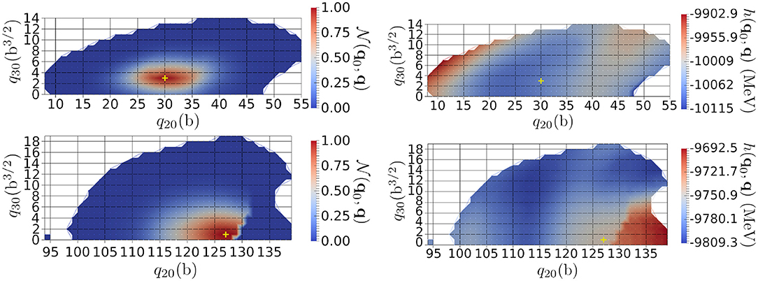
Figure 1. (Left) Overlaps ${N}(q_0,q)$ as a function of q and where q₀ = (30, 3), in barn units, corresponds to the ground state (upper panel) or q₀ = (127, 1), in barn units, which corresponds to a point at higher elongation (lower panel). This was obtained for a ²⁴⁰Pu nucleus. The white parts correspond to values below a threshold of 1.0 × 10⁻⁴. The yellow crosses correspond to q₀. (Right) Same as the corresponding left panels for the reduced energy kernel h(q₀, q).

This behavior is at the heart of the Gaussian Overlap Approximation, discussed in more detail in section 3. The reduced Hamiltonian h(q₀, q), defined as the ratio between the collective Hamiltonian and the norm kernel

$\begin{array}{ll}h(q_0,q)=\frac{\langle \varphi (q_0)\left|\widehat{H}\right|\varphi (q)\rangle }{\langle \varphi (q_0)|\varphi (q)\rangle },& (33)\end{array}$

has also been calculated for all overlaps greater than ϵ_thresh. In this work, only the kinetic and central terms of the interaction were included. The right panels of Figure 1 presents the slices of the reduced Hamiltonian for the same cases as in its left panels. The relative variation of the reduced Hamiltonian (where the norm kernel above the threshold) is almost constant, being only 2% around the ground state and 1% for the elongated configuration. In addition to the overlaps rapid decrease discussed above, it numerically justifies the standard second-degree polynomial approximation of this quantity (a further study with all the terms of the interaction is, however, required). The bottom panels highlight a discontinuous behavior around q₂₀ ≈ 130 b. This specific discontinuity is due to the existence of two competing valleys in the three-dimensional PES obtained by adding the hexadecapole moment $q_{40}=\langle {\widehat{Q}}_{40}\rangle$ as a collective DoF [38]. Such a discontinuity gives a similar label in the collective space to two HFB states that are far in the full many-body space. The Figure 2 is an illustration of such a discontinuity in a two-dimensional PES embedded in a three-dimensional collective space. It is not possible to reduce the loop ${C}$ to a point: the discontinuity is a hole whose edges are highlighted by the red line of Figure 2. Such a discontinuity may add spurious boundary effects in the description of the reaction of interest. It is especially the case when the discontinuity appears in an area of the collective space that gives important contributions to the targeted observables. Note that in approximate treatments such as the ones based on the Gaussian Overlap Approximation, discontinuities are always neglected, leading to a spurious connection between distant regions of the full many-body space.

FIGURE 2

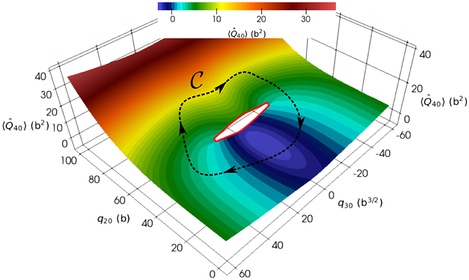
Figure 2. Schematic representation of a discontinuity in two-dimensional calculations with constraints on $q_{20}=\langle {\widehat{Q}}_{20}\rangle$ (x-axis) and $q_{30}=\langle {\widehat{Q}}_{30}\rangle$ (y-axis). The z-axis and the color scale are associated with the average values of the unconstrained hexadecapole moment $\langle {\widehat{Q}}_{40}\rangle$.

It is possible to determine the time evolution of the weight function f(q, t) of the GHW ansatz (3). In cases where the size of the discretized space of the collective coordinate is still tractable, this task has been achieved through a direct diagonalization of the collective Hamiltonian [37]. For this two-dimensional application, the straightforward diagonalization involves a prohibitive numerical cost. It is still possible to use a Crank-Nicolson method to integrate in time the GHW equation (16). Figure 3 presents a snapshot at time t = 0.55 zs of the quantity ℙ(q, t) defined as

$\begin{array}{ll}\mathbb{P}(q,t)\equiv \langle \text{Ψ}(t)\left|(|\varphi (q)\rangle \langle \varphi (q)|)\right|\text{Ψ}(t)\rangle .& (34)\end{array}$

This corresponds to the probability to measure the system in the state |ϕ(q)〉³. Even though the simulation was a proof-of-concept, we see that the bottom of the asymmetric valley is slightly more populated than the other parts of the PES near scission. This leads mostly to asymmetric fission fragments, which is in agreement with experimental data [39, 40]. The GCM wavefunction evolves in a slightly non-local way in the collective space (in the range of the width of the overlaps along q − q′), leading to non-zero probability “drops” appearing and disappearing along the time-evolution of the system.

FIGURE 3

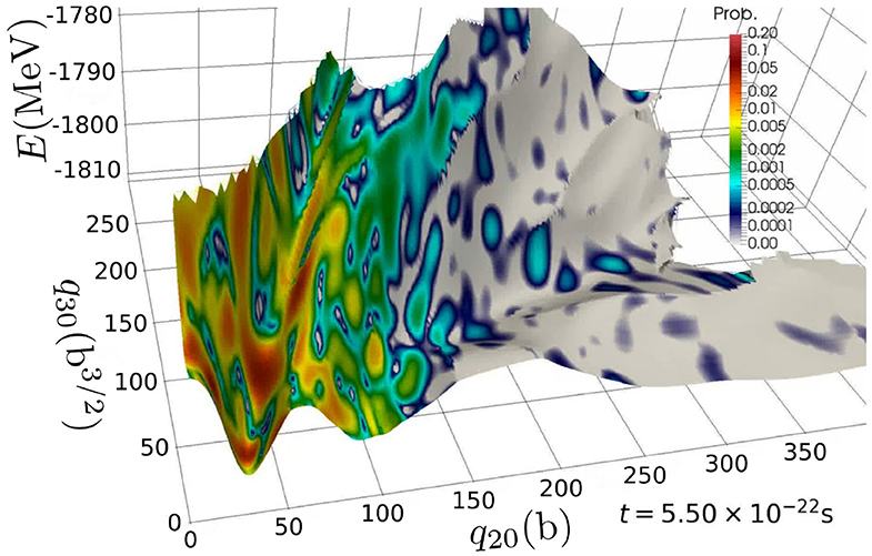
Figure 3. The gray surface represents the generator states' HFB energy as a function of q₂₀ and q₃₀. On top of this, the color map gives the quantity ℙ(q, t = 0.550zs) in the same conditions than those of Figure 1.

The most time-consuming part was the calculation of the norm and Hamiltonian kernels that required the use of 512 cpus for two weeks (~ 170, 000 cpu.h). The calculation of the time-evolution of the weight function f(q, t) for times up to 0.55zs was done using 64 cpus for one week (~ 10, 000 cpu.h). The short length of time for which the weight function was determined is not enough for the calculation of mass and charge probability distributions. A more realistic calculation would require at least 200, 000 cpu.h, for the determination of the weight function up to 10zs only.

The principal difficulty of such an application stems from the big size of the discretized space of the collective coordinates (substantially bigger, for example, than in the case of the static GCM calculations for nuclear structure). This makes the computation of the norm and Hamiltonian kernel intensive but still embarrassingly parallel. Besides, in the case of fission, techniques to determine the post-scission observables of the fragments still need to be developed for the exact TDGCM. For instance, some simplifying hypotheses on the way to treat open domains of collective coordinates are commonly used under the Gaussian Overlap Approximation [41] but are no longer valid in the exact TDGCM framework.

3. Gaussian Overlap Approximation (GOA)

In its straightforward application, the TDGCM leads to a non-local equation of motion that must be solved in a high-dimensional space in most of the practical calculations. As mentioned in Sec. 2, solving this equation involves a high numerical cost that strongly hurdles its applications in nuclear physics. Several approximate treatments of the TDGCM have been developed with the aim to build a local equation of motion for the collective wave function g(q, t) (cf. Equation 30). The Gaussian overlap approximation (GOA) is one of these approximations, which leverages the fact that the overlap and Hamiltonian kernels can, in some cases, be parameterized in terms of Gaussians of the variable q. In its static form, the GOA has been largely used and applied for nuclear structure. Especially, it provides a nice bridge between the Bohr Hamiltonian equation that was first formulated in [42] and a quantum treatment based on the 3A + A nucleons degrees of freedom [43–47]. Extensive reviews of the static version of the GOA can be found in [16, 48]. We focus here on its time-dependent flavor.

3.1. TDGCM+GOA With Time Even Generator States

3.1.1. Main Assumptions

In its most standard form, the GOA framework assumes the following situation:

1. we have a family of normed generator states {|ϕ(q)〉} parameterized by a vector of real coordinates q ∈ ℜ^m;

2. all the states of the set are time-even, i.e., they are their own symmetric by the time-reversal operation;

3. the function q → |ϕ(q)〉 is continuous and twice derivable;

4. the overlap between two arbitrary generator states can be approximated by a Gaussian shape

$\begin{array}{ll}{N}(q,q^{\prime })\simeq exp\left[-\frac{1}{2}{(q-q^{\prime })}^{t}G(\bar{q})(q-q^{\prime })\right],& (35)\end{array}$

with $\bar{q}=(q+q^{\prime })/2$ and $G(\bar{q})$ a real positive definite matrix;

5. the Hamiltonian kernel can be approximated by

$\begin{array}{ll}{H}(q,q^{\prime })\simeq {N}(q,q^{\prime })h(q,q^{\prime }),& (36)\end{array}$

where h(q, q′), a polynomial of degree two in the collective variables q and q′, is the reduced Hamiltonian.

In most applications of the TDGCM+GOA, the generator states are built as constrained Hartree-Fock-Bogoliubov states of even-even nuclei which ensures the time even property. The question is then: what are the situations where the Gaussian shape approximation is verified within a small error? Already from the time-reversal symmetry, we can infer that the overlaps are real and symmetric in (q − q′). Therefore, the following relation is satisfied in the vicinity of q

$\begin{array}{ll}\langle \varphi (q+\frac{s}{2})|\varphi (q-\frac{s}{2})\rangle =\text{exp }\left[\text{ln }\left(\langle q+\frac{s}{2}|q-\frac{s}{2}\rangle \right)\right].& (37)\end{array}$

A Taylor development of this expression up to order two in s already yields locally a Gaussian shape without any additional assumption

$\begin{array}{ll}\langle \varphi (q+\frac{s}{2})|\varphi (q-\frac{s}{2})\rangle =\text{exp }\left[-\frac{1}{2}{s}^{t}G(q)s+o(s^2)\right]& (38)\end{array}$

with

$\begin{array}{ll}{G}_{ij}(q)=\langle {\partial }_i\varphi (q)|{\partial }_j\varphi (q)\rangle ,& (39)\end{array}$

$\begin{array}{ll}|{\partial }_i\varphi \left(q\right)\rangle ={\frac{\partial |\varphi \left(a\right)\rangle }{\partial a_i}|}_q.& (40)\end{array}$

We used here some identities coming from the fact that generator states are normalized. In situations where the coordinates correspond to some collective deformations of the nucleus, it turns out that the Gaussian shape holds for larger values of s. This is justified from the central limit theorem in [48] for Slater determinants or in [16] for Bogoliubov vacua. It especially holds for heavy nuclei.

Finally, note that although we limit here our description to the case of time-even generator states, it is possible to build a GOA framework without assuming this symmetry. Such a generalization can be found, for instance, in [48].

3.1.2. Equation of Motion

Starting from the GOA hypothesis, one can reduce the equation of motion (30) to a local equation involving the first and second-order derivatives of the collective wave function. In this section, we give only the main ideas to derive this local equation. For more exhaustive demonstrations, we refer the reader to [16, 48, 49].

In its historical version, the GOA framework assumes that the width of the Gaussian shape is constant. However, in most of the practical cases, this assumption is too restrictive. To overcome this issue, a series of papers published in the 70–80's generalized the GOA framework to account for a varying Gaussian width [49–51]. The idea is to perform a change of collective variables to recover the constant width case. The mapping between the new collective coordinates α and the original ones q reads

$\begin{array}{ll}\alpha (q)={\displaystyle {\int }_{a\in C_0^q}}{G}^{\frac{1}{2}}(a)\text{d}a& (41)\end{array}$

where $C_0^q$ is a path from the origin to q. With this new labeling of the generator states, we get ⁴

$\begin{array}{ll}\langle \varphi \left(\alpha \right)|\varphi \left({\alpha }^{\prime }\right)\rangle \simeq \text{exp }\left[-\frac{1}{2}{\left(\alpha -{\alpha }^{\prime }\right)}^2\right].& (42)\end{array}$

We can therefore perform all the derivations with the α coordinates and make the inverse transformation on the final expressions only.

Starting with this simple form of the overlap, we seek an equation of motion involving a local collective Hamiltonian in the collective coordinate representation. The Gaussian shape of the norm kernel allows expressing its positive Hermitian square root analytically as

$\begin{array}{ll}{{N}}^{1/2}(\alpha ,{\alpha }^{\prime })=C·\text{exp }\left[-{(\alpha -{\alpha }^{\prime })}^2\right],& (43)\end{array}$

where the constant C only depends on the dimension of the coordinate α. Additionally, there is a simple link, involving Hermite polynomials, between the successive derivatives of a Gaussian shape and its multiplication by polynomials. For instance, we have for the two first derivatives in α

$\begin{array}{ll}\frac{\partial {{N}}^{1/2}}{\partial {\alpha }_k}=-2\left({\alpha }_k-{{\alpha }^{\prime }}_k\right){{N}}^{1/2},& (44)\end{array}$

$\begin{array}{ll}\frac{{\partial }^2{{N}}^{1/2}}{\partial {\alpha }_k\partial {\alpha }_l}=\left[-2{\delta }_{kl}+4({\alpha }_k-{\alpha }_k^{\prime })({\alpha }_l-{\alpha }_l^{\prime })\right]{{N}}^{1/2}.& (45)\end{array}$

In the following, we build a local collective Hamiltonian. After the change of variable (41), the Hamiltonian kernel between two arbitrary GHW states reads

$\begin{array}{l}\langle \text{Ψ}\left|\widehat{H}\right|\Phi \rangle \\ \begin{array}{l}={\displaystyle {\int }_{\alpha {\alpha }^{\prime }\xi }}{f}_{\text{Ψ}}^{\star }(\alpha ){{N}}^{1/2}(\alpha ,\xi )h(\alpha ,{\alpha }^{\prime }){{N}}^{1/2}(\xi ,{\alpha }^{\prime })f_{\Phi }({\alpha }^{\prime })\text{d}\alpha \text{ d}{\alpha }^{\prime }\text{ d}\xi .\end{array}& (46)\end{array}$

By assuming that the reduced Hamiltonian is a second-degree polynomial, we can write down for any point ξ

$\begin{array}{l}h(\alpha ,{\alpha }^{\prime })=h(\xi ,\xi )+h_{\alpha }(\alpha -\xi )+h_{{\alpha }^{\prime }}({\alpha }^{\prime }-\xi )\\ +\frac{1}{2}\left[h_{\alpha \alpha }{\left(\alpha -\xi \right)}^2+2h_{\alpha {\alpha }^{\prime }}\left(\alpha -\xi \right)\left({\alpha }^{\prime }-\xi \right)+h_{{\alpha }^{\prime }{\alpha }^{\prime }}{\left({\alpha }^{\prime }-\xi \right)}^2\right],& (47)\end{array}$

where h_α is a shorthand notation for the vector of the first derivatives of the reduced Hamiltonian estimated at ξ

$\begin{array}{ll}{h}_{\alpha }\equiv \left(\frac{\partial h(\alpha ,{\alpha }^{\prime })}{\partial {\alpha }_1}{|}_{\alpha ={\alpha }^{\prime }=\xi },\dots ,\frac{\partial h(\alpha ,{\alpha }^{\prime })}{\partial {\alpha }_m}{|}_{\alpha ={\alpha }^{\prime }=\xi }\right).& (48)\end{array}$

Similarly h_αα, $h_{\alpha {\alpha }^{\prime }}$, and $h_{{\alpha }^{\prime }{\alpha }^{\prime }}$ are the tensors of second derivatives with respect to the collective coordinates and evaluated at point ξ. The idea is then to inject this local development into equation (46). Using the relation (44), we express the reduced kernel as a local operator containing derivatives acting on the right-hand side ${{N}}^{1/2}$. Finally, after rearranging all the terms and performing some integrations by parts, we obtain the expected result

$\begin{array}{ll}\langle \text{Ψ}\left|\widehat{H}\right|\Phi \rangle ={\displaystyle {\int }_{\alpha {\alpha }^{\prime }}}{g}_{\text{Ψ}}^{\star }(\alpha )\tilde{{H}}(\alpha )\delta (\alpha -{\alpha }^{\prime })g_{\Phi }({\alpha }^{\prime })\text{d}\alpha \text{ d}{\alpha }^{\prime }.& (49)\end{array}$

The identification of this expression with (29) shows that the collective Hamiltonian is local. It reduces to a standard kinetic-plus-potential Hamiltonian acting on the collective wave function

$\begin{array}{ll}\tilde{{H}}(\alpha )=-\frac{{\hslash }^2}{2}{\nabla }_{\alpha }B(\alpha ){\nabla }_{\alpha }+V(\alpha ).& (50)\end{array}$

The potential and inertia matrices in this coordinate representation are ⁵

$\begin{array}{l}V(\alpha )=h(\alpha ,\alpha )-\frac{1}{2}\text{Tr}(h_{\alpha {\alpha }^{\prime }})\\ B(\alpha )=\frac{1}{2{\hslash }^2}(h_{\alpha {\alpha }^{\prime }}-h_{\alpha \alpha }).& (51)\end{array}$

Injecting this expression of the collective Hamiltonian into (30) and solving the resulting equation gives the time-evolution of the unknown function g(α). The ultimate step is to transform back this equation of motion to another one acting on the original set of coordinates q. Doing so, we get the same equation with a transformed local collective Hamiltonian

$\begin{array}{ll}\tilde{{H}}(q)=-\frac{{\hslash }^2}{2\sqrt{\gamma (q)}}{\nabla }_q\left[\sqrt{\gamma (q)}B(q)\right]{\nabla }_q+V(q).& (52)\end{array}$

The new collective Hamiltonian involves a metric γ(q) defined by

$\begin{array}{ll}\gamma (q)=\text{det }\left(G(q)\right).& (53)\end{array}$

The inertia tensor takes the more involved form

$\begin{array}{ll}B\left(q\right)=\frac{1}{2{\hslash }^2}{G}^{-1}\left(q\right)\left[h_{q{q}^{\prime }}-h_{qq}+{\displaystyle \sum _n{\Gamma }^n\left(q\right)h_{q_n}}\right]G^{-1}\left(q\right).& (54)\end{array}$

The notation Γⁿ(q) stands for the Christoffel symbol. It is a matrix related to G(q) through the relation

$\begin{array}{ll}{\Gamma }_{kl}^n(q)=\frac{1}{2}{\displaystyle \sum _i}{G}_{ni}^{-1}\left(\frac{\partial G_{ki}}{\partial q_l}+\frac{\partial G_{il}}{\partial q_k}-\frac{\partial G_{lk}}{\partial q_i}\right).& (55)\end{array}$

Finally, the potential becomes in this set of coordinate

$\begin{array}{ll}V(q)=h(q,q)-\frac{1}{2}\text{Tr}\left(G^{-1}(q)h_{q{q}^{\prime }}\right).& (56)\end{array}$

The first term is the HFB energy of the generator state |ϕ(q)〉. The second term is a zero-point correction that contains second derivatives of the reduced Hamiltonian. With some additional work, it is possible to express this zero-point correction ϵ_ZPE in a slightly more practical form that involves the inertia tensor and second derivatives of the energy h(q, q) only

$\begin{array}{l}{ϵ}_{\text{ZPE}}(q)=-\frac{{\hslash }^2}{2}\text{Tr}(BG)-\frac{1}{8}\text{Tr }\left(G^{-1}\frac{{\partial }^{2}h(q,q)}{\partial q^2}\right)\\ \begin{array}{l}+\frac{1}{8}\text{Tr }\left(G^{-1}{\displaystyle \sum _n}{\Gamma }^n\frac{\partial h(q,q)}{\partial a_n}\right).\end{array}& (57)\end{array}$

The equation of evolution (30) along with the expression of the collective Hamiltonian (52) and its components (53), (56), and (54) define the dynamics of the system in the TDGCM+GOA framework.

3.1.3. Inertia and Metric

The inertia tensor and the metric are quantities that depend on the derivatives of the generator states and the reduced Hamiltonian. One possibility could be to determine these derivatives numerically, for instance, with a finite difference method. In the standard situation where the generator states are constrained HFB solutions, one can find an analytical expression of the inertia and the metric. We recall here this result at any point q

$\begin{array}{ll}G=\frac{1}{2}{\left[{\text{M}}^{(1)}\right]}^{-1}{\text{M}}^{(2)}{\left[{\text{M}}^{(1)}\right]}^{-1}.& (58)\end{array}$

$\begin{array}{ll}B={\text{M}}^{(1)}{\left[{\text{M}}^{(2)}\right]}^{-1}{\tilde{\text{M}}}^{(1)}{\left[{\text{M}}^{(2)}\right]}^{-1}{\text{M}}^{(1)}.& (59)\end{array}$

The moments M^(K) and ${\tilde{\text{M}}}^{(K)}$ involve the QRPA matrix ${M}$ of the state |ϕ(q)〉 and are defined in Appendix 7.1. For the complete derivation of these results, we refer the reader to [52] and references therein. Note that this result neglects the term involving the Christoffel symbol in the inertia. The argument for this approximation relies on the slow variation of the metric according to the collective coordinates. We are not aware of the systematic verification of the validity of this assumption in applications.

In all TDGCM+GOA practical applications, the so-called perturbative cranking approximation is used to avoid a costly inversion of the QRPA matrix required to compute the metric and inertia. It consists in approximating the QRPA matrix by a diagonal part only, in the quasiparticle basis that diagonalizes the generalized density matrix of |ϕ(q)〉. This gives a simple and well known form for the moments M^(K)

$\begin{array}{ll}{M}_{ij}^{(K)}={\tilde{M}}_{ij}^{(K)}=\Re 𝔢{\displaystyle \sum _{\mu \nu }}\frac{\langle \mu \nu \left|{\widehat{Q}}_i\right|\varphi (q)\rangle \langle \varphi (q)\left|{\widehat{Q}}_j\right|\mu \nu \rangle }{{(E_{\mu }+E_{\nu })}^K},& (60)\end{array}$

where |μν〉 is a two quasiparticles excitation built on top of the generator state, and E_μ and E_ν are the corresponding quasiparticle energies.

The GCM+GOA framework unambiguously defines the metric and inertia as functions of the successive derivatives of the generator states and reduced Hamiltonian. However, it is known that this inertia and its approximate perturbative cranking estimation is too low to describe several situations correctly. One example is the case of a translation motion [48]. Several studies compare the GOA inertia with inertia provided by other theories yielding an equivalent collective equation of motion, such as quantized ATDHFB [53–55]. In [56], the authors extend the TDGCM+GOA framework by introducing conjugate coordinates that bring time odd components into the generator states. In particular, they show that the resulting collective Hamiltonian takes the same form as Equation (52) but where the ATDHFB inertia replaces the GOA inertia. This justifies the common practice of using the ATDHFB inertia when solving the collective equation of motion.

3.2. Applications in Nuclear Reactions

3.2.1. Low Energy Ion Collisions

The force of TDGCM+GOA is its versatility in the choice of collective coordinates and its ability to treat in the same framework the nucleons DoFs as well as more collective DoFs. It seems an appropriate way to tackle the dynamics of low energy ion collisions where the principal degree of freedom is the relative distance between the two reaction partners and where the collision affects the internal organization of the nucleons. It is possible to build a family of generator states along this line, describing the two reaction partners and parameterizing them by their relative distance. Several papers followed this idea during the 1980s. In particular, Berger and Gogny [57] treated the frontal collision of ¹²C+¹²C within a GCM+GOA approach. This kind of study focuses on the determination of the cross-section resonances for some specific output channels of the reaction. Figure 4 shows a typical result where the resulting positions of the resonances are compared to available experimental data. The predictions give a rough estimation of the position of the 0⁺ resonances, but they mostly fail to reproduce the presence of other resonances and their energy spacing. Many lacunae of the theory could explain such discrepancy, including the rough treatment of angular momentum, the breaking of some symmetries, or the mostly adiabatic characteristic of the GCM built on constrained HFB solutions.

FIGURE 4

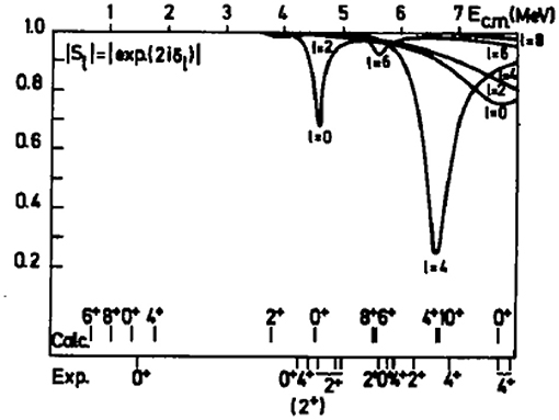
Figure 4. Reflection coefficients as a function of the center of mass energy (in MeV) of a ¹²C+¹²C head-on collision. The position of the resonances estimated from a GCM+GOA framework are compared to a set of experimental data. Figure taken from [57].

Other similar studies have been performed on the base of the GCM (without the GOA) and have made the connection to the resonating group method. Baye and Salmon looked at the ¹⁶O+⁴⁰Ca back angles scattering [58] along with the work of Friedrich et al. [59]. Also, Goeke et al. studied the ¹⁶O+¹⁶O collision in the framework of the quantized adiabatic time-dependent Hartree-Fock approach which yields a collective equation of motion identical to the one of TDGCM+GOA [60].

After this series of applications, treating collisions with the TDGCM+GOA framework was progressively abandoned to the profit of other methods such as the time-dependent Hartree-Fock plus pairing [61]. One difficulty that could explain this transition is the numerical cost required to build the generator states at the self-consistent mean-field level (note that this cost is nowadays completely acceptable). Beyond this, deeper problems raised, for instance, by the conservation of the total angular momentum of the collision or the generation of a continuous manifold of generator states appear with this method. Overall, the resulting cross-sections give only rough and qualitative estimations of the experimental data. The position of resonances, as well as the absolute value of cross-sections, are both observables that are very challenging to predict due to their extreme sensitivity to the kinematics of the reaction as well as the internal structure of the nuclei.

3.2.2. Fission Dynamics

The prediction of the fission fragments characteristics from a dynamical description is a domain where the TDGCM+GOA performs successfully. Fission involves heavy nuclei and begins with large collective motions that are mostly adiabatic. These two factors make the TDGCM+GOA framework built on constrained HFB solutions a suitable candidate. Moreover, the important width of the measured fission yields is the fingerprint of large quantum fluctuations of the one-body density of the compound system. Handling these fluctuations is precisely the purpose of the GCM.

The quest to predict fission yields from a dynamical TDGCM+GOA calculation began in the 1980s with the work of Berger et al. exploring the rupture of the neck between prefragments in terms of different collective coordinates [62, 63]. The first calculation of the mass distribution of fission fragments was later on performed among the same group for ²³⁸U [41]. The authors have described the fissioning system's dynamics using the two collective coordinates: q₂₀ and q₃₀ associated with the quadrupole and octupole moments of the compound nucleus. The [64] reports the same technique applied to a few other actinides with a qualitative reproduction of the experimental values. Younes and Gogny further proposed an alternative set of collective variables in [65]. Still, an impediment to this approach was its numerical cost, from the determination of the generator states (up to 40, 000 states in a 2-dimensional description) to the time integration of the collective Schrödinger equation. The development of new tools based on state-of-the-art numerical methods enables today's continuation of this work. For instance, the code FELIX [66, 67] solves the collective GOA dynamics efficiently based on a spectral element method. Also, the use of Bayesian processes to determine the best-suited parameters of a harmonic oscillator basis induced a significant speedup of some Hartree-Fock-Bogoliubov solvers.

In the last couple of years, we have seen a fast increase in the number of fission studies relying on this technique. All papers focused on the actinide region emphasize similar results. In this region, the potential energy landscape presents mostly one asymmetric fission valley. The exact topology of this surface reflects the internal organization of the nucleons that would correspond to the shell effects in a microscopic-macroscopic picture. By starting from a collective state localized in the low deformation first potential well, the dynamics mostly populates the configurations of the asymmetric channel. The left panel of Figure 5 shows the resulting yields obtained on an experimentally well-known nucleus, namely ²⁴⁰Pu.

FIGURE 5

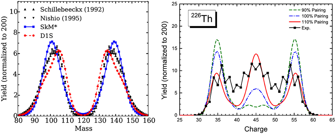
Figure 5. (Left) Fragment mass distribution for the low energy neutron induced fission ²³⁹Pu(n,f). Two TDGCM results obtained with the Gogny D1S and Skyrme SkM^* effective interactions are compared to two sets of experimental data. Reprinted figure with permission from [68]. Copyright 2016 by the American Physical Society. (Right) Fragment charge distribution obtained for a low energy fission of ²²⁶Th. The TDGCM+GOA results based on the relativistic mean field PC-PK1 with different pairing strengths are compared to experimental data (black line with points). Reprinted figure with permission from [69]. Copyright 2017 by the American Physical Society.

The TDGCM+GOA captures within a few mass units the position of the asymmetric peaks that are, in fact, mostly determined by the position of the asymmetric valley in the collective space. A similar quality of results has been obtained with the same method for other actinides, such as ²³⁶U or ²⁵²Cf. Finally, this framework seems to be able to describe the transitions between symmetric and asymmetric fissions that are measured outside of the actinide region. The left panel of Figure 6 shows the prediction versus experiment comparison of such a transition in the neutron-rich Fermium isotopes [70]. In this chain of isotopes, the addition of a few neutrons to ²⁵⁴Fm changes the dominant fragmentation mode completely. This can be interpreted as different shell effects occurring because of the new neutrons, that change the potential energy of the intermediate configurations leading to fission. This perturbation favors the population of the symmetric mode for ²⁵⁸Fm.

FIGURE 6

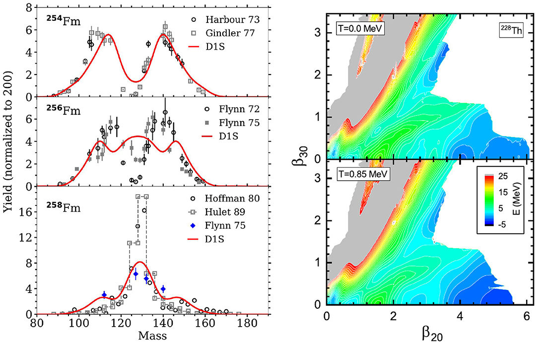
Figure 6. (Left) Primary fragment mass yields of Fermium isotopes obtained with the Gogny D1S effective interaction and compared with various experimental data sets after neutron evaporation. The open symbols stand for experimental data associated with spontaneous fission, whereas full symbols are related to thermal neutron-induced fission. Reprinted figure with permission from [70]. Copyright 2019 by the American Physical Society. (Right) Effect of temperature on the free energy surface of ²²⁸Th in the plane of deformation (β₂₀, β₃₀). Reprinted figure with permission from [73]. Copyright 2019 by the American Physical Society.

Several ingredients of the TDGCM+GOA framework for fission are still not adequately controlled and bring significant uncertainties on its predictions. Zdeb et al. [71] investigated in detail the impact of the choice of the initial state of the dynamics on the fission observables. They showed in particular that the global features of the fission yields (mostly the position and width of the peaks) are quite resilient to changes in the energy or the parity of the initial state. Furthermore, Tao et al. computed the fission yields from a relativistic mean-field approach [69] and looked at the sensitivity of the results to the pairing strength. The right panel of Figure 5 gives a clue of their results, showing the variation of the charge yields induced by a 10% variation of their nominal pairing strength in the case of the multimodal fission of ²²⁶Th. For this nucleus, we see that the pairing strength is an essential factor that drives the ratio between the yields of the symmetric and asymmetric modes. Finally, the same team explored the inclusion of temperature into the generator states as a way to better account for the diabatic aspects of the dynamics [72, 73]. The Figure 6 (right panel) shows that warming up the generator states changes slightly the topology of the potential energy surface. Increasing the temperature generally tends to smear out the shell effects and the structures in the potential energy surface. In the case of ²²⁶Th, it favors the symmetric fission and reduces the height of the asymmetric peaks of the mass yields by a factor ≃1.4.

Other components or approximations of the TDGCM+GOA, such as the perturbative cranking approximation for the collective inertia, may also bring their source of bias and uncertainty on the prediction.

3.3. Main Limitations

Despite its success in determining the fission fragment distribution, the TDGCM+GOA framework suffers from several shortcomings.

First, on the same ground as the exact TDGCM, its derivation relies on the knowledge of a many-body Hamiltonian. However, in all practical applications, it is used with an energy density functional (cf. section 2.5). Indeed, the GOA method does not require an explicit calculation of the off-diagonal elements of the energy kernel responsible for divergent behavior in GCM. However, the GOA's formal construction still depends on the existence and sound mathematical definition of these matrix elements to be a valid framework. In that sense, the GOA suffers from the same flaws as the exact TDGCM concerning the use of energy density functionals.

A second issue comes from the requirement that the function q → |ϕ(q)〉 is continuous and twice differentiable. The latter is a necessary condition to develop the formalism and, in particular, to compute the GOA metric and inertia. However, the standard construction of the family of generator states from constrained HFB solutions does not guaranty this property [38]. Different studies highlight discontinuities of this function in the treatment of fission, similar to the one visible in Figure 1. In the common (q₂₀, q₃₀) space of collective coordinates, a line of discontinuity is present in the vicinity of scission configurations. This feature limits the domain of validity of the collective dynamics and ultimately prevents the determination of the fission fragments characteristics after their complete separation.

Finally, we have seen that most of the current applications of TDGCM+GOA rely on constrained HFB solutions for the generator states. Certain diabatic aspects of the nuclear dynamics are then difficult to grasp with the corresponding GHW many-body wave function. This is the case of the dissipation as well as the viscosity of the shape dynamics predicted with Langevin methods [74, 75] or time-dependent Hartree-Fock-Bogoliubov calculations. Past and ongoing studies to improve the description of these effects include efforts to quantize the Langevin equation [76, 77], to couple the Langevin dynamics with the GCM [78] or to couple TDHFB trajectories with TDGCM [79]. Other techniques, such as the SCIM and TDGCM based on time-dependent generator states, are also promising avenues that we discuss in this review.

4. Schrödinger Collective-Intrinsic Model (SCIM)

Intrinsic degrees of freedom are often neglected in the microscopic modeling of the dynamics of reactions. However, including intrinsic degrees of freedom in a static GCM framework has already been performed, for instance, in [80, 81]. These studies show that taking into account two-quasiparticle excitations significantly improves the prediction of high spin levels, such as the 6⁺ states in medium mass isotopes as well as the prediction for β excitation bands and its transition probabilities to other rotational bands in heavier systems. On another topic, the TDHFB/SLDA methods [82, 83] and semi-classical approaches to the description of fission [84, 85] clue that dissipation (and therefore intrinsic degrees of freedom) are necessary to describe the fission fragments properties correctly. Therefore, a few collective degrees of freedom are not enough to adequately model such a reaction. Several paths can be taken to overcome this limitation without resorting to the determination of an exact solution of the GHW Equation (16). A strategy in development consists in using the TDGCM+GOA with finite-temperature inertia tensors and collective potential. However, the inclusion of statistical mechanics on top of the TDGCM framework still lacks a solid formalization. The idea of the Schrödinger Collective-Intrinsic Model (SCIM) [86–88] is to derive a local Schrodinger-like equation from a generalization of the GHW ansatz (3) that contains individual quasiparticle degrees of freedom. The transformation to a local equation relies on the symmetric moment expansion method [89, 90]. The full SCIM formalism can be found in [86–88] in the stationary case. However, we would like to present here a derivation of the time-dependent SCIM equations consistent with the ones given for the TDGCM and the TDGCM+GOA equations.

4.1. Main Assumptions

The SCIM involves four main assumptions. The first one is the expression of the state |Ψ(t)〉 that describes the evolution of the many-body wavefunction associated with the reaction. This expression is assumed to be a generalization of the GHW ansatz

$\begin{array}{ll}|\psi \left(t\right)\rangle ={\displaystyle \sum _k{\displaystyle \int \text{}\text{d}q|{\varphi }_k\left(q\right)\rangle }}{f}_k(q,t).& (61)\end{array}$

In [87], the authors consider a family of generator states associated with one collective coordinate q defined as the quadrupole moment of the system. The index k iterates over the labels of the sheets of collective space which correspond, in this case, to two quasiparticle excitations. Figure 7 shows the evolution of the excitation energies of the non-adiabatic points of the potential energy surface of ²³⁶U.

FIGURE 7

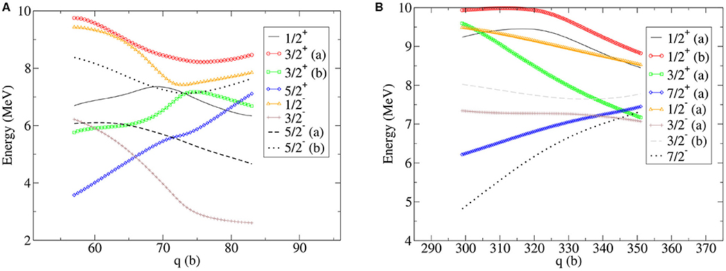
Figure 7. (Color online) Excitation energies as a function of the quadrupole moment constraint q and associated with 2-qp excitations of HFB states. The system under study is ²³⁶U around $\langle {\widehat{Q}}_{20}\rangle =70$ b (A) and $\langle {\widehat{Q}}_{20}\rangle =325$ b (B). The figures are taken from [86].

Note that the scope of expression (61) is broader than the only explicit inclusion of intrinsic DoF in the formalism. For example, it is used for K-mixing in the context of stationary angular-momentum-projected GCM on a triaxial configuration basis. In this case, the index k iterates over the values of K. The second assumption is the analyticity of the weight function f of the GCM ansatz (61) that allows the symmetrization of the GHW equations. The third assumption is the vanishing of the weight function and its derivatives at the boundaries of the integration domain. An implicit corollary of this property is the continuity of the functions q → |ϕ_k(q)〉. It turns out that this assumption is in practice not verified for a broad range of applications, for example, in the actinide region, as emphasized in section 3.3. These three assumptions lead to the symmetrized GHW equation

$\begin{array}{ll}{\displaystyle \sum _k{\displaystyle \int \text{d}}}\text{}s{e}^{is{P}/2}\left[{H}{[s]}_{lk}(q)-i{N}{[s]}_{lk}(q)\frac{\text{d}\text{}}{\text{d}\text{}t}\right]e^{is{P}/2}{f}_k(q,t)=0,& (62)\end{array}$

where the following notations are introduced

$\begin{array}{ll}{H}{\left[s\right]}_{lk}(q)={{H}}_{lk}(q+s/2,q-s/2)& (63)\end{array}$

$\begin{array}{ll}{N}{\left[s\right]}_{lk}(q)={{N}}_{lk}(q+s/2,q-s/2),& (64)\end{array}$

and where the Hermitian operator

$\begin{array}{ll}{P}=i\frac{\partial }{\partial q}& (65)\end{array}$

corresponds to the conjugate moment associated with the collective variables. The symmetrized GHW equation can be written in a more compact operator format as

$\begin{array}{ll}{\displaystyle \int \text{d}}\text{}s{e}^{is{P}/2}\left[{H}[s]-i{N}[s]\frac{\text{d}\text{}}{\text{d}\text{}t}\right]e^{is{P}/2}\text{f}(t)=0,& (66)\end{array}$

where f(t) denotes the function q ↦ f_k(q, t). The fourth and last assumption of the SCIM is the validity of the truncation of the symmetric moment expansion (SME) of the norm and Hamiltonian kernels of (66) up to order two. It was, for instance, verified numerically in the context of the study [87]. The SME of ${K}={N},{H}$, in the case of one collective variable,

$\begin{array}{ll}{K}={\displaystyle \sum _n}\frac{1}{n!}{\left\{{{K}}^{(n)},{P}\right\}}^{(n)},& (67)\end{array}$

is obtained through the properties of the so-called Symmetric Ordered Product of Operators (SOPO) ${\left\{{{K}}^{(n)},{P}\right\}}^{(n)}$ presented in Appendix 8 where ${{K}}^{(n)}$ is the moment of order n of ${K}\left[s\right]$ in the variable s

$\begin{array}{ll}{{K}}^{(n)}\equiv i^n{\displaystyle \int }\text{d}s{s}^n{K}\left[s\right].& (68)\end{array}$

The properties of the SOPO used to obtain these expressions are listed in Appendix 8.

The expression (67) can be generalized to the case of m collective variables,

$\begin{array}{ll}{K}={\displaystyle \sum _n}\frac{1}{n!}{\left\{{{K}}^{(n)},{P}\right\}}^{(n)},& (69)\end{array}$

where the index n iterates over all the m-tuples of positive integers and where we have introduced the following notations

$\begin{array}{ll}n!\equiv n_0!n_1!\cdots n_{m-1}!& (70)\end{array}$

$\begin{array}{ll}{\left\{{K},{P}\right\}}^{\left(n\right)}\equiv {\left\{\cdots {\left\{{\{{K},{{P}}_0\}}^{\left(n_0\right)},{{P}}_1\right\}}^{\left(n_1\right)}\cdots ,{{P}}_{m-1}\right\}}^{\left(n_{m-1}\right)}& (71)\end{array}$

$\begin{array}{ll}{{K}}^{(n)}\equiv {\displaystyle \int }\text{d}s\left[{\displaystyle \prod _k}{(i{s}_k)}^{n_k}\right]{K}\left[s\right].& (72)\end{array}$

Their second-order approximation in their SME development is then given by

$\begin{array}{ll}{N}\approx {\displaystyle \sum _{\overline{n}\le 2}\frac{1}{n!}}{\left\{{{N}}^{\left(n\right)},{P}\right\}}^{\left(n\right)}& (73)\end{array}$

$\begin{array}{ll}{H}\approx {\displaystyle \sum _{\overline{n}\le 2}\frac{1}{n!}}{\left\{{{H}}^{\left(n\right)},{P}\right\}}^{\left(n\right)}& (74)\end{array}$

where $\bar{n}$ is the sum of the elements of n. In the one-dimensional case, the expressions reduce to.

$\begin{array}{ll}{N}\approx {\displaystyle \sum _{n=0}^2}\frac{1}{n!}{\left\{{{N}}^{(n)},{P}\right\}}^{(n)},& (75)\end{array}$

$\begin{array}{ll}{H}\approx {\displaystyle \sum _{n=0}^2}\frac{1}{n!}{\left\{{{H}}^{(n)},{P}\right\}}^{(n)}.& (76)\end{array}$

4.2. Schrodinger Collective-Intrinsic Equation

The Schrödinger-like expression of the SCIM equations is given by

$\begin{array}{ll}\left[{{H}}^{\text{CI}}-i\frac{\text{d}}{\text{d}t}\right]\text{ g}(t)=0,& (77)\end{array}$

where g(t) is defined according to

$\begin{array}{ll}g(t)={{N}}^{1/2}\text{f}(t)& (78)\end{array}$

and normalized as

$\begin{array}{ll}{g}^{†}(t)\text{g}(t)={\displaystyle \int }\text{d}q{g}^{\star }(q,t)g(q,t)=1.& (79)\end{array}$

The operator ${{N}}^{1/2}$ is the only positive-definite hermitian square-root of ${{N}}^{1/2}$ and ${{N}}^{-1/2}$ is the inverse of the latter. Finally, using the hermicity of ${{N}}^{-1/2}$, the collective-intrinsic Hamiltonian ${{H}}^{\text{CI}}$ has the expression

$\begin{array}{ll}{{H}}^{\text{CI}}={{N}}^{-1/2}{H}{{N}}^{-1/2}.& (80)\end{array}$

An explicit form for ${{H}}^{\text{CI}}(q)$ is given by

$\begin{array}{ll}{{H}}^{\text{CI}}=\frac{1}{2}{\left\{{B},{P}\right\}}^{(2)}+{\left\{{T},{P}\right\}}^{(1)}+{V},& (81)\end{array}$

where the expressions of ${U}={B}/2$, ${T}$ and ${V}$ are given in [86–88]. By analogy with the TDGCM+GOA collective Hamiltonian (52), the first term of (81) can be interpreted as a kinetic term and ${B}$ as the inertia tensor, related to the mass tensor ${M}$ through the relation

$\begin{array}{ll}{B}={{M}}^{-1}.& (82)\end{array}$

Similarly, the third term of (81) is comparable to the potential term of the TDGCM+GOA. However, the last term

$\begin{array}{ll}{\left\{{T},{P}\right\}}^{(1)}=\frac{1}{2}\left[{T}\frac{\partial }{\partial q}+\frac{\partial }{\partial q}{T}\right],& (83)\end{array}$

contains first-order derivatives according to the collective variable, at the opposite of the TDGCM+GOA. In the Langevin equations, such a term corresponds to viscosity and arises in the SCIM from the coupling between intrinsic and collective degrees of freedom.

4.3. Choice of Quasiparticle Excitations

In [86–88], the generator states consist in

• constrained HFB states $|{\varphi }_{k=0}(q=\langle {\widehat{Q}}_{20}\rangle )\rangle$ describing the compound system at different elongations,

• intrinsic excitations of these HFB states

$\begin{array}{ll}|{\varphi }_{k>0}(q)\rangle =\widehat{X}{(q)}_k|{\varphi }_0(q)\rangle .& (84)\end{array}$

Note that the specific expression of $\widehat{X}{(q)}_k$ is never used in the derivations of the Schrodinger-like equation, and it is only assumed that all the states in the collective space are time-reversal to avoid complex-valued overlaps. In practice, the intrinsic excitations taken into account in the existing developments of SCIM are considering 2-qp excitations. The included HFB states are breaking the rotational and particle number symmetries. In order to avoid restoring these symmetries, the quasiparticle excitations are chosen according to the following rules

1. the operators ${\widehat{X}}_k$ are two quasiparticles operators,

2. all the states in the collective space have to be time-reversal invariant,

3. the chosen excitations have to preserve “as much as possible” the number of particles and K, the projection of the total angular moment on the symmetry axis,

4. and they must be associated with an excitation energy below 10 MeV.

The time-reversal condition limits the possible excitation operators to be

$\begin{array}{ll}\widehat{X}{\left(q\right)}_k={\alpha }_k{\widehat{\eta }}_{k_1}^{(q)†}{\widehat{\eta }}_{{\overline{k}}_2}^{(q)†}-{\widehat{\eta }}_{{\overline{k}}_1}^{(q)†}{\widehat{\eta }}_{k_2}^{(q)†}& (85)\end{array}$

$\begin{array}{ll}{\alpha }_k=\frac{1}{\sqrt{2}}\left(1+{\delta }_{k_1,k_2}\left(1-\frac{1}{\sqrt{2}}\right)\right),& (86)\end{array}$

where ${\widehat{\eta }}_{k_1}^{(q)†}$ is the creation operator of the quasiparticle k₁ associated with the HFB state

$\begin{array}{ll}|{\varphi }_0(q)\rangle ={\displaystyle \prod _l{\widehat{\eta }}_l^{\left(q\right)}|0\rangle .}& (87)\end{array}$

Additionally, the selected quasiparticles in $\widehat{X}{(q)}_k$ are assumed to have the same projection on the total angular moment on the symmetry axis K_k1 = K_k2 so that the K of the total system is unchanged. In case the HFB states are obtained with preserved parity, the same condition on π is added.

Couplings between collective and intrinsic excitations play a major role in many reactions. For instance, it is known to play a crucial role in the distribution of excitation energy between the nascent fragments produced by fission. The TDGCM+GOA enables a microscopic description of nuclear reactions without internal degrees of freedom, while Langevin-based methods allow the semi-classical description of the reaction with the inclusion of thermal effects. The SCIM leads to a local Schrodinger-like equation, much simpler to solve than the exact, non-local, Griffin-Hill-Wheeler equation while being based on fewer assumptions than the TDGCM+GOA or Langevin. The collective-intrinsic Hamiltonian includes a viscosity term that is known to be relevant to the description of nuclear reaction from Langevin's calculations. However, the method still involves the full calculation of the norm and Hamiltonian kernels, which is extremely time-consuming. Furthermore, the formalism is rather complex compared to other methods such as the TDGCM+GOA. At present, this method did not lead to any application beyond the works presented in [86–88], and still needs to be tested thoroughly against experimental data.

5. Quantum Mixture of Time-Dependent States

In its standard form, the TDGCM relies on the ansatz (3) that expands the many-body wave function on a family of time-independent generator states. The dynamics of the system is, therefore, entirely carried out by the time evolution of the collective wave function g(q) driven by Equation 30. Although successful in describing some nuclear phenomena like collective vibrations, such an expansion suffers from two significant drawbacks.

The first one resides in the large dimension of the ensemble of generator states required to describe processes like nuclear reactions correctly. Despite the efforts reported in sections 3 and 4 to reduce the collective Hamiltonian to a local approximation, this high dimension quickly becomes a hindrance to the numerical applications of TDGCM. An origin of this difficulty is the fact that all the many-body configurations populated at any time of the reaction must be represented in the set of generator states. In many situations, this expansion is not optimal in the sense that most of the associated weights are close to zero at a given time. To give an example, we may consider the translation motion of a localized particle. While the translated states at any positions are to be incorporated in a TDGCM description of its motion, the collective wave function at a given time only has a small spatial expansion. A natural idea is then to express the wave function as a linear superposition of a few time-dependent states that follow the expected particle's translation motion. It may even happen that one well-chosen time-dependent basis state is enough to describe the dynamics of the system very accurately. The time-dependent energy density functional treatment of the giant resonances in nuclear physics provides such an example [91, 92].

The second drawback of the TDGCM is the construction of a family of generator states before the determination of the system evolution. The equation of motion provides only the probability of the system to populate parts of this predefined space. For this approach to work, the physicist must rely on an a priori knowledge of the relevant states for the dynamics. For nuclear reactions, it typically means that one should correctly guess what will be the reaction's output channels and include an ensemble of states representative of these channels in the working space. Beyond the difficulty to generate states representative of the systems far from the initial state, the typical risks of this method are

• to miss important channels/states in the construction of the set of generator states,

• to include states that will not be populated at all but will still increase the numerical cost.

A solution to overcome these difficulties is the expansion of the ansatz (3) on a set of time-dependent states, as shown schematically in Figure 8. In this case, the many-body wave function of the system reads

$\begin{array}{ll}|\Psi (t)\rangle ={\displaystyle {\int }_{q\in E}f}(q,t)|\varphi \left(q,t\right)\rangle .& (88)\end{array}$

This very general ansatz brings more flexibility as the configuration basis can vary in time. However, this flexibility comes with additional complexity in the equation of motion for the collective wavefunction g(q, t) and the generator states |ϕ(q, t)〉. Studies in both chemistry and nuclear physics are exploring different strategies in the choice of generator states and the determination of the equation of motion of the system. We review these recent efforts in this section.

FIGURE 8

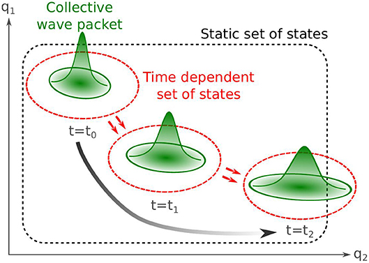
Figure 8. Schematic dynamics of a localized collective wave packet. With the TDGCM strategy (static set of generator states), most of the working space does not contribute, and part of the final state is not captured. In contrast, a small, well-chosen set of time-dependent states is sufficient to capture the system's dynamics entirely.

5.1. The Multiconfiguration Time-Dependent Hartree-Fock Approach

In 1990, Meyer et al. introduced the multiconfiguration time-dependent Hartree (MCTDH) approach to tackle the dynamics of molecules [93]. Contrary to the fermionic many-body problem, the system's degrees of freedom are distinct from each other and correspond typically to distances between some atoms of a molecule. Their associated wave function is assumed to be at any time a mixture of product states

$\begin{array}{ll}|\Psi (x_1,\cdots ,x_n,t)\rangle ={\displaystyle \sum _{i_1=0}^{m_1-1}\cdots }{\displaystyle \sum _{i_n=0}^{m_n-1}{c}_{i_1\cdots i_n}}\times |{\phi }_{i_1}^{(1)}(t)\rangle \cdots |{\phi }_{i_n}^{(n)}(t)\rangle ,& (89)\end{array}$

where at any time, the $\{|{\phi }_{i_k}^{(k)}(t)\}$ form a basis of the space associated with the kth degree of freedom, and the c_i1⋯in are the mixing coefficients between all the product states. The equation of motion of both the individual states and the mixing coefficients can then be obtained from applying the Dirac-Frenkel variational principle. This method was since applied to different dynamical processes in chemistry [94–96] and up to five degrees of freedom in the treatment of the inelastic cross-section of H₂O + H₂ [97]. Note that in 2003, Wang et al. proposed an extension of this method referred to as multilayers MCTDHF to tackle more degrees of freedom (up to a few thousand) [98].

A natural extension of this work to the fermionic many-body problem is the replacement of the product states by Slater determinants in the trial wavefunction. This extension was introduced in [99] and the new ansatz reads

$\begin{array}{ll}|\Psi (r_1,\cdots ,r_n,t)\rangle ={\displaystyle \sum _{i_1=0}^{m_1-1}\cdots }{\displaystyle \sum _{i_n=0}^{m_n-1}{c}_{i_1\cdots i_n}|}{\varphi }_{i_1\cdots i_n}(t)\rangle ,& (90)\end{array}$

with the time-dependent Slater determinants

$\begin{array}{ll}|{\varphi }_{i_1\cdots i_n}(t)\rangle ={\widehat{a}}_{i_1}^{†}(t)\cdots {\widehat{a}}_{i_n}^{†}(t)|0\rangle .& (91)\end{array}$

In this expression, ${â}_{i_k}^{†}(t)$ stands for the fermionic creation operator of a particle in a single-particle state |φ_ik(r, t)〉. This many-body wave function can then be injected into a time-dependent variational principle whose parameters are both the mixing coefficients c_i1⋯in and the single-particle wave functions |φ_ik〉. Note that there is no one-to-one mapping between the many-body state |ψ(t)〉 and the parameters of the right-hand side. In practical applications, the set of single-particle wave functions is assumed to be orthonormal at any time

$\begin{array}{ll}\langle {\phi }_i(t)|{\phi }_j(t)\rangle ={\delta }_{ij}.& (92)\end{array}$

This criterion lets some freedom in the choice of the c_ik and |φ_ik〉 for a given many-body wave function, leading to an additional degree of freedom in their associated equation of motion. A usual convention to fix this freedom consists in imposing the additional constraint

$\begin{array}{ll}\langle {\phi }_i(t)\left|\frac{\partial }{\partial t}\right|{\phi }_j(t)\rangle =0.& (93)\end{array}$

This choice stabilizes the single-particle states against rotations among the occupied states. If such rotation has to be described, only the mixing coefficients will be affected while the single-particle states will stay constant. This convention yields to equations of motion that are often more suited for the numerical time integration.

With this criterion, the Dirac-Frenkel variational principle applied to a two-body Hamiltonian system leads to the equation of motion for both the coefficients and the single-particle states

$\begin{array}{ll}i\hslash {ċ}_{i_1\cdots i_n}(t)={\displaystyle \sum _{i_1=0}^{m_1-1}}\cdots {\displaystyle \sum _{i_n=0}^{m_n-1}}\langle {\varphi }_{i_1\cdots i_n}(t)\left|\widehat{H}\right|{\varphi }_{i_1\cdots i_n}(t)\rangle c_{i_1\cdots i_m}(t)& (94)\end{array}$

$\begin{array}{ll}i\hslash |{\stackrel{.}{\phi }}_n(t)\rangle =\widehat{P}\left\{\widehat{t}|{\phi }_n(t)\rangle +{\displaystyle \sum _{pqrs}{({\rho }^{-1})}_{np}{\rho }_{qspr}^{(2)}{\widehat{h}}_{rs}|{\phi }_q(t)\rangle }\right\}& (95)\end{array}$

where $\widehat{t}$ is the one-body part of the Hamiltonian, ĥ is the mean-field potential that implicitly depends on the one-body density, ρ and ρ⁽²⁾ are the one- and two-body density matrices and $\widehat{P}$ is a projection operator on the orthogonal complement of the occupied single-particle states. Such equation of motions have then been numerically solved for chemical systems with six valence electrons [99], to study the two photons ionization of helium [100] or the dynamics of di-molecular molecules [101, 102]. In nuclear physics, the multiconfiguration Hartree-Fock approach has been applied in its static version to determine the structure of light nuclei mostly in the s-d shell [103, 104]. Such an expansion of the many-body state enables a good description of the low lying excitation spectrum with typically the first 2⁺ excitation reproduced within a few 100 keV. For the ground-state binding energy, this work still emphasizes a significant overestimation of the theory by 8.3 MeV in average in the s-d shell nuclei. This discrepancy would mostly come from (i) double-counting coming from the usage of energy functional that have been fitted at the mean-field level, (ii) the truncation of the configuration space that still cuts too early the population of single-particle states with the largest spatial expansion. Even though it would be interesting to study photoabsorption phenomena in light nuclei or diffusion between light nuclei, this method has not yet been applied in its dynamics version for nuclear physics. A generalization of the ansatz (90) to a superposition of Bogoliubov vacua and its corresponding equation of motion is yet to be formalized and tested.

5.2. Multiconfiguration With Time-Dependent Non Orthogonal States

The trial state of Equation (90) at the core of the MCTDHF method expands the wave function on a set of orthonormal Slater determinants. The orthonormality between such generator states simplifies the equation of motion as typically the norm kernel defined in Equation (6) is the identity at any time. In contrast, it may be more efficient in some situations to expand the many-body wave function on a set of non-orthogonal generator states (i.e., time-dependent Bogoliubov vacua with time-dependent deformations). Such a strategy was explored, for instance, in chemistry by mixing TDDFT trajectories with a shift in time to include memory effect [105] into the dynamics. This approach was proven to correctly include the description of dissipation in the two electrons dynamics of a Hooke's atom.

In nuclear physics, the idea of mixing time-dependent TDHF trajectories was already proposed in 1983 in the pioneering work of Reinhard et al. [106] to treat nuclear collisions. Starting back from the ansatz (90), the authors proposed to take as the time-dependent generator states a set of TDHF trajectories starting from different initial conditions. A time-dependent variational principle is then applied to obtain the equation of motion only for the mixing function f(q, t) (or the collective wave function g(q, t)). Such a principle is schematically pictured in Figure 9 (left panel).

FIGURE 9

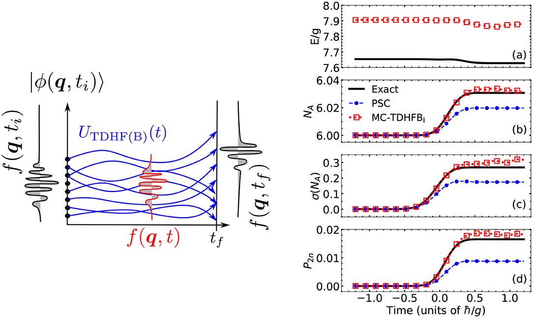
Figure 9. (Left) Schematic picture of a GCM mixing of TDHF(B) trajectories. (Right) Evolution of several observables during the dynamics of a simple model of collision between two superfluids. The total energy (a), the number of particles in the left subsystem (b), and its dispersion (c) as well as the probability to transfer one pair of fermions during the collision (d) are plotted against the time of the collision for the exact many-body solution (black line), a statistical mixture of TDHFB trajectories (blue circles) and a quantum mixture of the same TDHFB trajectories (red squares). Reprinted figure with permission from [107]. Copyright 2019 by the American Physical Society.

The idea behind this scheme is that the TDHF trajectories will carry most of the one-body dynamics of the system, whereas the weight function will encompass part of the two-body collisional dynamics, in such importance as to account for additional dissipation and fluctuation. In this paper, a GOA approximation was performed to determine the evolution of the collective wave function in a one-dimensional nuclear collision model. The results showed in particular that the widths of the internal excitation energy of the collision partners after the collision were increased by a factor of seven compared to a TDHF trajectory alone. This additional fluctuation is directly coming from the additional correlations tackled by the enriched ansatz for the many-body wave function.

Even though promising, applications of this method to realistic systems were not carried out. One possible explanation is the numerical cost associated with TDHF trajectories. However, the advances in numerical methods and the recent development of supercomputers induced a surge of interest for such studies. In particular, the inclusion of superfluidity in our time-dependent mean-field codes [82, 108] opened the possibility to predict collisions between open-shell nuclei. Along this line, Scamps et al. attempted to predict the transfer of pairs of fermions in the contact between two superfluids based on a statistical mixing of TDHFB trajectories [109–111]. The idea is that the one-body dynamics of the nuclear processes would be already well accounted for by TDHFB like trajectories, while a statistical ensemble of such trajectories would account for the additional fluctuation induced by the residual two-body collisions terms of the dynamics. Up to now, these methods were only tested on toy-model cases and collisions between a few light systems such as ²⁰O+²⁰O. Experimental data on such collisions still lack, which prevents a rigorous theory versus experiment comparison.

Nevertheless, the tests on exactly solvable models show that these semiclassical approaches manage to recover some crucial fluctuation related to the relative gauge angle between the reaction partners. In particular, they can predict the probability of one pair transfer with the proper order of magnitude in the perturbative regime where the nuclear interaction during the collision is weak compared to the pairing forces acting in each subsystem. Still, they partially miss the quantum interference between the TDHFB trajectories. Depending on the method's details, this may either lead to underestimating fluctuations of one-body observables or, in the worse case, predicting unphysical behavior such as particle transfer after the re-separation of the two reaction partners.

Coming back to a full quantum treatment of the problem, Regnier et al. recently attempted the full-fledged mixing of TDHFB trajectories in [107]. In this context, the time-dependent variational principle on the ansatz 90 leads to the equation of motion of the collective wave function g(q, t)

$\begin{array}{ll}\begin{array}{c}i\hslash \stackrel{.}{g}=\left(\tilde{{H}}-\tilde{{D}}+i\hslash {\stackrel{.}{{N}}}^{1/2}{{N}}^{-1/2}\right)g.\end{array}& (96)\end{array}$

This equation involves the collective operators $\tilde{{H}}$ and $\tilde{{D}}$ defined by the application of Equation (28) on the kernels

$\begin{array}{ll}{H}(q,q^{\prime })=\langle \varphi (q,t)\left|\widehat{H}\right|\varphi (q^{\prime },t)\rangle ,& (97)\end{array}$

$\begin{array}{ll}{D}(q,q^{\prime })=\langle \varphi (q,t)|i\hslash \frac{\partial }{\partial t}|\varphi (q^{\prime },t)\rangle .& (98)\end{array}$

All the kernels and collective operators involved now depend on time. Compared to the TDGCM on static generator states (Equation 30), this equation contains two additional terms. The first one contains the time derivative of the generator states, whereas the second one is linked to the time derivative of the norm kernel. These equations were numerically solved only in a simple case modeling the contact between two superfluid systems. The main results are summarized in the right panel of Figure 9. The full black line represents the system's exact many-body dynamics, and it is compared with a prediction obtained from a statistical mixture of TDHFB trajectories (the PSC method, dashed blue line) as well as the quantum mixing of the same TDHFB trajectories. While the statistical method recovers the good order of magnitude for most predictions, the inclusion of interference between the TDHFB trajectories significantly improves these results. In particular, a factor of two is highlighted between each method's predictions of the probability P_2n to transfer a pair of fermions during the collision.

At a time where performing series of independent time-dependent mean-field calculations in nuclear physics becomes possible, such a method could be a suitable candidate to tackle nuclear reactions with a complex interplay between one-body and many-body degrees of freedom. The caveat to its direct application on a realistic nuclear collision would still be the difficulty that current implementations of the nuclear mean-field dynamics formalisms rely on energy density functionals instead of a linear Hamiltonian (cf. section 2.5).

6. Conclusion

This review presents four variants of the Time-Dependent Generator Coordinates Method that is rooted in a configuration-mixing principle. This class of methods is of particular interest to microscopically describe heavy-fermion systems. It allows the physicist to focus the description on the correlations of interest through the choice of the collective coordinates. Most of the time, the collective coordinates are related to some of the first multipole moments of the intrinsic one-body density or some groups of symmetry operators. Such freedom makes the TDGCM extremely versatile. Still, its practical applications in nuclear physics are plagued by the usage of effective Hamiltonians or energy density functionals that lead to misbehaviors of the energy kernel, an essential ingredient shared by all the TDGCM approaches.

The Time-Dependent Generator Coordinate Method is the most direct implementation of the configuration-mixing principle. In this case, the only approximations are the expression of the nuclear Hamiltonian, and the restriction of the total Fock space to the one spanned by the configuration basis. The Griffin-Hill-Wheeler (GHW) Equation (3) is the corresponding equation of motion. The main limitation of this method arises from the non-locality of the GHW equation in the collective coordinates representation, leading to intensive parallel computation. By resorting to some approximations, it is possible to rewrite the GHW equations into local equations, reducing hereafter substantially the calculation needs. The Gaussian Overlap Approximation (GOA) transforms the GHW equations to a local Schrodinger-like equation essentially under the condition that the norm kernel is of Gaussian character. The TDGCM+GOA is the most widely used implementation of the TDGCM for the description of nuclear reactions and especially for fission. The Schrodinger Collective-Intrinsic Method is based on the truncation of the GHW equation in the second-order to obtain a local Schrodinger-like equation. In its current form, it still requires to calculate the full norm and Hamiltonian kernels. Finally, it is possible to generalize the standard TDGCM approach by expanding the many-body wave function on a set of time-dependent generator states. The recent progress of TDHFB solvers opens new possibilities for practical applications along this line.

Overall, most of these methods were first developed in the 1980s, at a time when they were quickly facing intractable numerical costs. The computational power at our disposal nowadays is an incentive to revisit the TDGCM approaches and look for new opportunities in the description of nuclear reactions. One of the most significant challenges in this path is the determination of energy density functionals or effective Hamiltonians, which are compatible with the GCM formalism and yield quantitative predictions of nuclear observables.

Author Contributions

All authors listed have made a substantial, direct and intellectual contribution to the work, and approved it for publication.

Funding

This work was performed at Los Alamos National Laboratory under the auspices of the National Nuclear Security Administration of the U.S. Department of Energy at Los Alamos National Laboratory under Contract No. 89233218CNA000001. Support for this work was provided through the Fission In R-process Elements (FIRE) Topical Collaboration in Nuclear Theory of the U.S. Department of Energy. It was partly performed under the auspices of the U.S. Department of Energy by the Lawrence Livermore National Laboratory (LLNL) under Contract No. DE-AC52-07NA27344.

Conflict of Interest

The authors declare that the research was conducted in the absence of any commercial or financial relationships that could be construed as a potential conflict of interest.

Acknowledgments

The authors would like to thank N. Schunck for his patience through the writing process of this paper as well as for fruitful comments on the manuscript.

Footnotes

1. ^For some applications, it may be convenient to add one or several discrete generator coordinates. We will then note the generator states as |ϕ_k(q)〉 where k is a vector of discrete labels. A typical example of a discrete label could be the K quantum number associated with the projection of the total spin onto a symmetry axis of the nucleus. Another example is provided in section 4.

2. ^Note that such a definition is possible for any observable $\widehat{O}$ due to the property

$\begin{array}{l}{Q}{O}={O}.\end{array}$

3. ^Note that due to the non-orthogonality of the generator states its sum over all the points q is not equal to 1.

4. ^Note that this assumes (i) that the integrals of G^1/2(a) are independent of the integration path (ii) that its evaluation properly approximates the average of G^1/2 on the path at the central point of the path [51].

5. ^Note that some higher-order correction terms in the potential are neglected here [see [48] for more details].

References

1. Bohr N, Wheeler JA. The mechanism of nuclear fission. Phys Rev. (1939) 56:426–450. doi: 10.1103/PhysRev.56.426

CrossRef Full Text | Google Scholar

2. Bohr A, Mottelson BR. Nuclear Structure. Singapore; River Edge, NJ: World Scientific (1998). doi: 10.1142/3530-vol1

CrossRef Full Text | Google Scholar

3. Scheid W, Greiner W. Theory of projection of spurious center of mass and rotational states from many-body nuclear wave functions. Ann Phys. (1968) 48:493–525. doi: 10.1016/0003-4916(68)90143-7

CrossRef Full Text | Google Scholar

4. Fink B, Kolb D, Scheid W, Greiner W. Spurious rotational states in deformed nuclear shell models. Ann Phys. (1972) 69:375–99. doi: 10.1016/0003-4916(72)90182-0

CrossRef Full Text | Google Scholar

5. Hill DL, Wheeler JA. Nuclear constitution and the interpretation of fission phenomena. Phys Rev. (1953) 89:1102–45. doi: 10.1103/PhysRev.89.1102

CrossRef Full Text | Google Scholar

6. Griffin JJ, Wheeler JA. Collective motions in nuclei by the method of generator coordinates. Phys Rev. (1957) 108:311–27. doi: 10.1103/PhysRev.108.311

CrossRef Full Text | Google Scholar

7. Bender M. Going beyond the self-consistent mean-field with the symmetry-restored generator coordinate method: from single-reference toward multi-reference energy density functional theory. Eur Phys J Spec Top. (2008) 156:217–28. doi: 10.1140/epjst/e2008-00619-9

CrossRef Full Text | Google Scholar

8. Egido JL. State-of-the-art of beyond mean field theories with nuclear density functionals. Phys Scr. (2016) 91:073003. doi: 10.1088/0031-8949/91/7/073003

CrossRef Full Text | Google Scholar

9. Krewald S, Rosenfelder R, Galonska JE, Faessler A. Selfconsistent generator coordinate method for giant monopole resonances. Nucl Phys A. (1976) 269:112–24. doi: 10.1016/0375-9474(76)90400-0

CrossRef Full Text | Google Scholar

10. Stoitsov MV, Ring P, Sharma MM. Generator coordinate calculations for breathing-mode giant monopole resonance in the relativistic mean-field theory. Phys Rev C. (1994) 50:1445–55. doi: 10.1103/PhysRevC.50.1445

PubMed Abstract | CrossRef Full Text | Google Scholar

11. Caurier E, Bourotte-Bilwes B, Abgrall Y. Microscopic treatment of the coupled monopole and quadrupole vibrations in light nuclei. Phys Lett B. (1973) 44:411–5. doi: 10.1016/0370-2693(73)90321-3

CrossRef Full Text | Google Scholar

12. Flocard H, Vautherin D. Generator coordinate calculations of giant resonances with the Skyrme interaction. Nucl Phys A. (1976) 264:197–220. doi: 10.1016/0375-9474(76)90428-0

CrossRef Full Text | Google Scholar

13. Abgrall Y, Caurier E. On the monopole and quadrupole isoscalar giant resonances in 4He, 16O, 20Ne and 40Ca. Phys Lett B. (1975) 56:229–31. doi: 10.1016/0370-2693(75)90381-0

CrossRef Full Text | Google Scholar

14. Vretenar D, Lalazissis GA, Behnsch R, Pöschl W, Ring P. Monopole giant resonances and nuclear compressibility in relativistic mean field theory. Nucl Phys A. (1997) 621:853–78. doi: 10.1016/S0375-9474(97)00192-9

CrossRef Full Text | Google Scholar

15. De Toledo Piza A, De Passos E. The kinematics of generator co-ordinates. Il Nuovo Cimento B. (1978) 45:1–30. doi: 10.1007/BF02904070

CrossRef Full Text | Google Scholar

16. Ring P, Schuck P. The Nuclear Many-Body Problem. Berlin: Springer Science & Business Media (2004).

Google Scholar

17. Löwdin PO, Mukherjee PK. Some comments on the time-dependent variation principle. Chem Phys Lett. (1972) 14:1–7. doi: 10.1016/0009-2614(72)87127-6

CrossRef Full Text | Google Scholar

18. Crank J, Nicolson P. A practical method for numerical evaluation of solutions of partial differential equations of the heat-conduction type. Adv Comput Math. (1996) 6:207–26. doi: 10.1007/BF02127704

CrossRef Full Text | Google Scholar

19. Reed M, Simon B. Methods of Modern Mathematical Physics. Princeton: Academic Press (1972).

Google Scholar

20. Robledo LM. Sign of the overlap of hartree-fock-bogoliubov wave functions. Phys Rev C. (2009) 79:021302. doi: 10.1103/PhysRevC.79.021302

CrossRef Full Text | Google Scholar

21. Anguiano M, Egido JL, Robledo LM. Particle number projection with effective forces. Nucl Phys A. (2001) 696:467–93. doi: 10.1016/S0375-9474(01)01219-2

CrossRef Full Text | Google Scholar

22. Lacroix D, Duguet T, Bender M. Configuration mixing within the energy density functional formalism: removing spurious contributions from nondiagonal energy kernels. Phys Rev C. (2009) 79:044318. doi: 10.1103/PhysRevC.79.044318

CrossRef Full Text | Google Scholar

23. Bender M, Duguet T, Lacroix D. Particle-number restoration within the energy density functional formalism. Phys Rev C. (2009) 79:044319. doi: 10.1103/PhysRevC.79.044319

CrossRef Full Text | Google Scholar

24. Duguet T, Bender M, Bennaceur K, Lacroix D, Lesinski T. Particle-number restoration within the energy density functional formalism: nonviability of terms depending on noninteger powers of the density matrices. Phys Rev C. (2009) 79:044320. doi: 10.1103/PhysRevC.79.044320

CrossRef Full Text | Google Scholar

25. Sheikh JA, Dobaczewski J, Ring P, Robledo LM, Yannouleas C. Symmetry restoration in mean-field approaches. arXiv [Preprint] arXiv:190106992. (2019).

Google Scholar

26. Ryssens W, Hellemans V, Bender M, Heenen PH. Solution of the Skyrme–HF+BCS equation on a 3D Mesh, II: a new version of the Ev8 code. Comput Phys Commun. (2015) 187:175–94. doi: 10.1016/j.cpc.2014.10.001

CrossRef Full Text | Google Scholar

27. Dönau F. Canonical form of transition matrix elements. Phys Rev C. (1998) 58:872–7. doi: 10.1103/PhysRevC.58.872

CrossRef Full Text | Google Scholar

28. Anguiano M, Egido JL, Robledo LM. Coulomb exchange and pairing contributions in nuclear Hartree–Fock–Bogoliubov calculations with the gogny force. Nucl Phys A. (2001) 683:227–54. doi: 10.1016/S0375-9474(00)00445-0

CrossRef Full Text | Google Scholar

29. Almehed D, Frauendorf S, Dönau F. Pairing correlations in high-K bands. Phys Rev C. (2001) 63:044311. doi: 10.1103/PhysRevC.63.044311

CrossRef Full Text | Google Scholar

30. Dobaczewski J, Stoitsov MV, Nazarewicz W, Reinhard PG. Particle-number projection and the density functional theory. Phys Rev C. (2007) 76:054315. doi: 10.1103/PhysRevC.76.054315

CrossRef Full Text | Google Scholar

31. Duguet T, Bonche P. Density dependence of two-body interactions for beyond-mean-field calculations. Phys Rev C. (2003) 67:054308. doi: 10.1103/PhysRevC.67.054308

CrossRef Full Text | Google Scholar

32. Robledo LM. Remarks on the use of projected densities in the density-dependent part of skyrme or gogny functionals. J Phys G: Nucl Part Phys. (2010) 37:064020. doi: 10.1088/0954-3899/37/6/064020

CrossRef Full Text | Google Scholar

33. Rodríguez-Guzmán R, Egido JL, Robledo LM. Correlations beyond the mean field in magnesium isotopes: angular momentum projection and configuration mixing. Nucl Phys A. (2002) 709:201–35. doi: 10.1016/S0375-9474(02)01019-9

CrossRef Full Text | Google Scholar

34. Bennaceur K, Idini A, Dobaczewski J, Dobaczewski P, Kortelainen M, Raimondi F. Nonlocal energy density functionals for pairing and beyond-mean-field calculations. J Phys G. (2017) 44:045106. doi: 10.1088/1361-6471/aa5fd7

CrossRef Full Text | Google Scholar

35. Yao JM, Bally B, Engel J, Wirth R, Rodríguez TR, Hergert H. Ab initio treatment of collective correlations and the neutrinoless double beta decay of 48Ca. arXiv:190805424. (2019). doi: 10.1103/PhysRevLett.124.232501

CrossRef Full Text | Google Scholar

36. Verriere M. Description de la Dynamique de la Fission Dans le Formalisme de la méthode de la Coordonnée génératrice dépendante du Temps. Université Paris-Saclay (2017). Available online at: https://tel.archives-ouvertes.fr/tel-01559158/document

Google Scholar

37. Verriere M, Dubray N, Schunck N, Regnier D, Dossantos-Uzarralde P. Fission description: first steps towards a full resolution of the time-dependent hill-wheeler equation. EPJ Web Conf. (2017) 146:04034. doi: 10.1051/epjconf/201714604034

CrossRef Full Text | Google Scholar

38. Dubray N, Regnier D. Numerical search of discontinuities in self-consistent potential energy surfaces. Comput Phys Commun. (2012) 183:2035–41. doi: 10.1016/j.cpc.2012.05.001

CrossRef Full Text | Google Scholar

39. Nishio K, Nakagome Y, Kanno I, Kimura I. Measurement of fragment mass dependent kinetic energy and neutron multiplicity for thermal neutron induced fission of plutonium-239. J Nucl Sci Technol. (1995) 32:404–14. doi: 10.1080/18811248.1995.9731725

CrossRef Full Text | Google Scholar

40. Tsuchiya C, Nakagome Y, Yamana H, Moriyama H, Nishio K, Kanno I, et al. Simultaneous measurement of prompt neutrons and fission fragments for 239Pu(nth,f). J Nucl Sci Technol. (2000) 37:941–8. doi: 10.1080/18811248.2000.9714976

CrossRef Full Text | Google Scholar

41. Goutte H, Berger JF, Casoli P, Gogny D. Microscopic approach of fission dynamics applied to fragment kinetic energy and mass distributions in U238. Phys Rev C. (2005) 71:024316. doi: 10.1103/PhysRevC.71.024316

CrossRef Full Text | Google Scholar

42. Bohr A. The coupling of nuclear surface oscillations to the motion of individual nucleons. Dan Mat Fys Medd. (1952) 26:1–40.

Google Scholar

43. Kumar K, Baranger M. Complete numerical solution of Bohr's collective Hamiltonian. Nucl Phys A. (1967) 92:608–52. doi: 10.1016/0375-9474(67)90636-7

CrossRef Full Text | Google Scholar

44. Libert J, Girod M, Delaroche JP. Microscopic descriptions of superdeformed bands with the Gogny force: configuration mixing calculations in the A≃190 mass region. Phys Rev C. (1999) 60:054301. doi: 10.1103/PhysRevC.60.054301

CrossRef Full Text | Google Scholar

45. Delaroche JP, Girod M, Libert J, Goutte H, Hilaire S, Péru S, et al. Structure of even-even nuclei using a mapped collective Hamiltonian and the D1S Gogny interaction. Phys Rev C. (2010) 81:014303. doi: 10.1103/PhysRevC.81.014303

CrossRef Full Text | Google Scholar

46. Fu Y, Mei H, Xiang J, Li ZP, Yao JM, Meng J. Beyond relativistic mean-field studies of low-lying states in neutron-deficient krypton isotopes. Phys Rev C. (2013) 87:054305. doi: 10.1103/PhysRevC.87.054305

CrossRef Full Text | Google Scholar

47. Matsuyanagi K, Matsuo M, Nakatsukasa T, Yoshida K, Hinohara N, Sato K. Microscopic derivation of the Bohr–Mottelson collective Hamiltonian and its application to quadrupole shape dynamics. Phys Scr. (2016) 91:063014. doi: 10.1088/0031-8949/91/6/063014

CrossRef Full Text | Google Scholar

48. Reinhard P, Goeke K. The generator-coordinate method and quantized collective motion in nuclear systems. Rep Prog Phys. (1987) 50:1–64. doi: 10.1088/0034-4885/50/1/001

CrossRef Full Text | Google Scholar

49. Krappe HJ, Pomorski K. Theory of Nuclear Fission. Springer (2012). Available online at: http://www.springer.com/us/book/9783642235146.

Google Scholar

50. Onishi N, Une T. Local Gaussian approximation in the generator coordinate method. Prog Theor Phys. (1975) 53:504–15. doi: 10.1143/PTP.53.504

CrossRef Full Text | Google Scholar

51. Gozdz A. An extended Gaussian overlap approximation in the generator coordinate method. Phys Lett B. (1985) 152:281–3. doi: 10.1016/0370-2693(85)90495-2

CrossRef Full Text | Google Scholar

52. Schunck N, Robledo LM. Microscopic theory of nuclear fission: a review. Rep Prog Phys. (2016) 79:116301. doi: 10.1088/0034-4885/79/11/116301

PubMed Abstract | CrossRef Full Text | Google Scholar

53. Holzwarth G. Four approaches to the function of inertia in a solvable model. Nucl Phys A. (1973) 207:545–64. doi: 10.1016/0375-9474(73)90861-0

CrossRef Full Text | Google Scholar

54. Góźdź A, Pomorski K, Brack M, Werner E. The mass parameters for the average mean-field potential. Nucl Phys A. (1985) 442:26–49. doi: 10.1016/0375-9474(85)90131-9

CrossRef Full Text | Google Scholar

55. Baran A, Sheikh J, Dobaczewski J, Nazarewicz W, Staszczak A. Quadrupole collective inertia in nuclear fission: cranking approximation. Phys Rev C. (2011) 84:054321. doi: 10.1103/PhysRevC.84.054321

CrossRef Full Text | Google Scholar

56. Reinhard PG, Goeke K. The generation coordinate method with conjugate parameters and its relation to adiabatic time-dependent hartree-fock. J Phys G. (1978) 4:L245. doi: 10.1088/0305-4616/4/9/006

CrossRef Full Text | Google Scholar

57. Berger J, Gogny D. A self-consistent microscopic approach to the 12C+ 12C reaction at low energy. Nucl Phys A. (1980) 333:302–32. doi: 10.1016/0375-9474(80)90235-3

CrossRef Full Text | Google Scholar

58. Baye D, Salmon Y. Generator-coordinate study of elastic 40Ca+ 40Ca scattering. Nucl Phys A. (1979) 323:521–39. doi: 10.1016/0375-9474(79)90123-4

CrossRef Full Text | Google Scholar

59. Friedrich H, Langanke K, Weiguny A. Elastic scattering of 16O on 40Ca at backward angles. Phys Lett B. (1976) 63:125–8. doi: 10.1016/0370-2693(76)90630-4

CrossRef Full Text | Google Scholar

60. Goeke K, Grümmer F, Reinhard PG. Three-dimensional nuclear dynamics in the quantized ATDHF approach. Ann Phys. (1983) 150:504–51. doi: 10.1016/0003-4916(83)90025-8

CrossRef Full Text | Google Scholar

61. Sekizawa K. TDHF Theory and its extensions for the multinucleon transfer reaction: a mini review. Front Phys. (2019) 7:20. doi: 10.3389/fphy.2019.00020

CrossRef Full Text | Google Scholar

62. Berger JF, Girod M, Gogny D. Microscopic analysis of collective dynamics in low energy fission. Nucl Phys A. (1984) 428:23–36. doi: 10.1016/0375-9474(84)90240-9

CrossRef Full Text | Google Scholar

63. Berger JF, Girod M, Gogny D. Time-dependent quantum collective dynamics applied to nuclear fission. Comput Phys Commun. (1991) 63:365–74. doi: 10.1016/0010-4655(91)90263-K

CrossRef Full Text | Google Scholar

64. Younes W, Gogny D. Fragment Yields Calculated in a Time-Dependent Microscopic Theory of Fission. Livermore, CA: Lawrence Livermore National Laboratory (2012). doi: 10.2172/1053671

CrossRef Full Text | Google Scholar

65. Younes W, Gogny D. Collective Dissipation from Saddle to Scission in a Microscopic Approach. Livermore, CA: Lawrence Livermore National Laboratory (2012). doi: 10.2172/1053675

CrossRef Full Text | Google Scholar

66. Regnier D, Verriére M, Dubray N, Schunck N. FELIX-1.0: a finite element solver for the time dependent generator coordinate method with the Gaussian overlap approximation. Comput Phys Commun. (2016) 200:350–63. doi: 10.1016/j.cpc.2015.11.013

CrossRef Full Text | Google Scholar

67. Regnier D, Dubray N, Verriére M, Schunck N. FELIX-2.0: new version of the finite element solver for the time dependent generator coordinate method with the Gaussian overlap approximation. Comput Phys Commun. (2018) 225:180–91. doi: 10.1016/j.cpc.2017.12.007

CrossRef Full Text | Google Scholar

68. Regnier D, Dubray N, Schunck N, Verriére M. Fission fragment charge and mass distributions in ²39Pu(n,f) in the adiabatic nuclear energy density functional theory. Phys Rev C. (2016) 93:054611. doi: 10.1103/PhysRevC.93.054611

CrossRef Full Text | Google Scholar

69. Tao H, Zhao J, Li ZP, Nikšić T, Vretenar D. Microscopic study of induced fission dynamics of Th 226 with covariant energy density functionals. Phys Rev C. (2017) 96:024319. doi: 10.1103/PhysRevC.96.024319

CrossRef Full Text | Google Scholar

70. Regnier D, Dubray N, Schunck N. From asymmetric to symmetric fission in the fermium isotopes within the time-dependent generator-coordinate-method formalism. Phys Rev C. (2019) 99:024611. doi: 10.1103/PhysRevC.99.024611

CrossRef Full Text | Google Scholar

71. Zdeb A, Dobrowolski A, Warda M. Fission dynamics of²52Cf. Phys Rev C. (2017) 95:054608. doi: 10.1103/PhysRevC.95.054608

CrossRef Full Text | Google Scholar

72. Zhao J, Nikšić T, Vretenar D, Zhou SG. Microscopic self-consistent description of induced fission dynamics: finite-temperature effects. Phys Rev C. (2019) 99:014618. doi: 10.1103/PhysRevC.99.014618

CrossRef Full Text | Google Scholar

73. Zhao J, Xiang J, Li ZP, Nikšić T, Vretenar D, Zhou SG. Time-dependent generator-coordinate-method study of mass-asymmetric fission of actinides. Phys Rev C. (2019) 99:054613. doi: 10.1103/PhysRevC.99.054613

CrossRef Full Text | Google Scholar

74. Usang MD, Ivanyuk FA, Ishizuka C, Chiba S. Correlated transitions in TKE and mass distributions of fission fragments described by 4-D Langevin equation. Sci Rep. (2019) 9:1–9. doi: 10.1038/s41598-018-37993-7

PubMed Abstract | CrossRef Full Text | Google Scholar

75. Miyamoto Y, Aritomo Y, Tanaka S, Hirose K, Nishio K. Origin of the dramatic change of fission mode in fermium isotopes investigated using Langevin equations. Phys Rev C. (2019) 99:051601. doi: 10.1103/PhysRevC.99.051601

CrossRef Full Text | Google Scholar

76. Parisi G, Wu YS. Perturbation theory without gauge fixing. Sci Sin. (1981) 24:483–96.

Google Scholar

77. Damgaard P, Tsokos K. Stochastic quantization with fermions. Nucl Phys B. (1984) 235:75–92. doi: 10.1016/0550-3213(84)90149-4

CrossRef Full Text | Google Scholar

78. Sadhukhan J, Nazarewicz W, Schunck N. Microscopic modeling of mass and charge distributions in the spontaneous fission of ²40Pu. Phys Rev C. (2016) 93:011304. doi: 10.1103/PhysRevC.93.011304

CrossRef Full Text | Google Scholar

79. Bulgac A, Jin S, Roche KJ, Schunck N, Stetcu I. Fission dynamics of 240Pu from saddle to scission and beyond. Phys Rev C. (2019) 100:034615. doi: 10.1103/PhysRevC.100.034615

PubMed Abstract | CrossRef Full Text | Google Scholar

80. Müther H, Goeke K, Allaart K, Faessler A. Single-particle degrees of freedom and the generator-coordinate method. Phys Rev C. (1977) 15:1467–76. doi: 10.1103/PhysRevC.15.1467

CrossRef Full Text | Google Scholar

81. Chen FQ, Egido JL. Triaxial shape fluctuations and quasiparticle excitations in heavy nuclei. Phys Rev C. (2017) 95:024307. doi: 10.1103/PhysRevC.95.024307

CrossRef Full Text | Google Scholar

82. Bulgac A, Magierski P, Roche KJ, Stetcu I. Induced fission of ²40Pu within a real-time microscopic framework. Phys Rev Lett. (2016) 116:122504. doi: 10.1103/PhysRevLett.116.122504

PubMed Abstract | CrossRef Full Text | Google Scholar

83. Bulgac A, Jin S, Stetcu I. Unitary evolution with fluctuations and dissipation. Phys Rev C. (2019) 100:014615. doi: 10.1103/PhysRevC.100.014615

CrossRef Full Text | Google Scholar

84. Sierk AJ. Langevin model of low-energy fission. Phys Rev C. (2017) 96:034603. doi: 10.1103/PhysRevC.96.034603

CrossRef Full Text | Google Scholar

85. Wada T, Carjan N, Abe Y. Multi-dimensional Langevin approach to fission dynamics. Nucl Phys A. (1992) 538:283–9. doi: 10.1016/0375-9474(92)90778-I

CrossRef Full Text | Google Scholar

86. Bernard R. Taking Into Account the Intrinsic Excitations and Their Couplings to Collective Modes in the Fission Process; Couplages Modes Collectifs - Excitations Intrinseques Dans le Processus de Fission. Université Pierre et Marie Curie (2011).

Google Scholar

87. Bernard R, Goutte H, Gogny D, Younes W. Microscopic and nonadiabatic Schrödinger equation derived from the generator coordinate method based on zero- and two-quasiparticle states. Phys Rev C. (2011) 84:044308. doi: 10.1103/PhysRevC.84.044308

CrossRef Full Text | Google Scholar

88. Younes W, Gogny DM, Berger JF. A Microscopic Theory of Fission Dynamics Based on the Generator Coordinate Method. Lecture Notes in Physics. Springer International Publishing (2019). Available online at: www.springer.com/us/book/9783030044220.

Google Scholar

89. Holzwarth G. The connection between the generator coordinate method and bose expansions. Nucl Phys A. (1972) 185:268–72. doi: 10.1016/0375-9474(72)90568-4

CrossRef Full Text | Google Scholar

90. Kerman AK, Koonin SE. Quantum theory of dissipation for nuclear collective motion. Phys Scr. (1974) 10:118–21. doi: 10.1088/0031-8949/10/A/020

CrossRef Full Text | Google Scholar

91. Scamps G, Lacroix D. Systematics of isovector and isoscalar giant quadrupole resonances in normal and superfluid spherical nuclei. Phys Rev C. (2013) 88:044310. doi: 10.1103/PhysRevC.88.044310

CrossRef Full Text | Google Scholar

92. Scamps G, Lacroix D. Systematic study of isovector and isoscalar giant quadrupole resonances in normal and superfluid deformed nuclei. Phys Rev C. (2014) 89:034314. doi: 10.1103/PhysRevC.89.034314

CrossRef Full Text | Google Scholar

93. Meyer HD, Manthe U, Cederbaum LS. The multi-configurational time-dependent Hartree approach. Chem Phys Lett. (1990) 165:73–8. doi: 10.1016/0009-2614(90)87014-I

CrossRef Full Text | Google Scholar

94. Manthe U, Meyer HD, Cederbaum LS. Wave-packet dynamics within the multiconfiguration Hartree framework: general aspects and application to NOCl. J Chem Phys. (1992) 97:3199–213. doi: 10.1063/1.463007

CrossRef Full Text | Google Scholar

95. Beck MH, Jäckle A, Worth GA, Meyer HD. The Multiconfiguration Time-Dependent Hartree (MCTDH) method: a highly efficient algorithm for propagating wavepackets. Phys Rep. (2000) 324:1–105. doi: 10.1016/S0370-1573(99)00047-2

CrossRef Full Text | Google Scholar

96. Meyer HD, Gatti F, Worth GA. Multidimensional Quantum Dynamics: MCTDH Theory and Applications. John Wiley & Sons (2009). doi: 10.1002/9783527627400

CrossRef Full Text | Google Scholar

97. Ndengué S, Scribano Y, Gatti F, Dawes R. State-to-state inelastic rotational cross sections in five-atom systems with the multiconfiguration time dependent Hartree method. J Chem Phys. (2019) 151:134301. doi: 10.1063/1.5119381

PubMed Abstract | CrossRef Full Text | Google Scholar

98. Wang H, Thoss M. Multilayer formulation of the multiconfiguration time-dependent Hartree theory. J Chem Phys. (2003) 119:1289–99. doi: 10.1063/1.1580111

PubMed Abstract | CrossRef Full Text | Google Scholar

99. Nest M, Klamroth T, Saalfrank P. The Multiconfiguration time-dependent Hartree–Fock method for quantum chemical calculations. J Chem Phys. (2005) 122:124102. doi: 10.1063/1.1862243

PubMed Abstract | CrossRef Full Text | Google Scholar

100. Hochstuhl D, Bonitz M. Two-photon ionization of helium studied with the multiconfigurational time-dependent Hartree–Fock method. J Chem Phys. (2011) 134:084106. doi: 10.1063/1.3553176

PubMed Abstract | CrossRef Full Text | Google Scholar

101. Kato T, Kono H. Time-dependent multiconfiguration theory for electronic dynamics of molecules in an intense laser field. Chem Phys Lett. (2004) 392:533–40. doi: 10.1016/j.cplett.2004.05.106

CrossRef Full Text | Google Scholar

102. Kato T, Kono H. Time-dependent multiconfiguration theory for electronic dynamics of molecules in intense laser fields: a description in terms of numerical orbital functions. J Chem Phys. (2008) 128:184102. doi: 10.1063/1.2912066

PubMed Abstract | CrossRef Full Text | Google Scholar

103. Robin C, Pillet N, Pe na Arteaga D, Berger JF. Description of nuclear systems with a self-consistent configuration-mixing approach: theory, algorithm, and application to the C 12 test nucleus. Phys Rev C. (2016) 93:024302. doi: 10.1103/PhysRevC.93.024302

CrossRef Full Text | Google Scholar

104. Robin C, Pillet N, Dupuis M, Le Bloas J, Pe na Arteaga D, Berger JF. Description of nuclear systems with a self-consistent configuration-mixing approach. II. Application to structure and reactions in even-even s d -shell nuclei. Phys Rev C. (2017) 95:044315. doi: 10.1103/PhysRevC.95.044315

CrossRef Full Text | Google Scholar

105. Orestes E, Capelle K, da Silva ABF, Ullrich CA. Generator coordinate method in time-dependent density-functional theory: memory made simple. J Chem Phys. (2007) 127:124101. doi: 10.1063/1.2768368

PubMed Abstract | CrossRef Full Text | Google Scholar

106. Reinhard PG, Cusson RY, Goeke K. Time evolution of coherent ground-state correlations and the TDHF approach. Nucl Phys A. (1983) 398:141–88. doi: 10.1016/0375-9474(83)90653-X

CrossRef Full Text | Google Scholar

107. Regnier D, Lacroix D. Microscopic description of pair transfer between two superfluid fermi systems. II. Quantum mixing of time-dependent Hartree-Fock-Bogolyubov trajectories. Phys Rev C. (2019) 99:064615. doi: 10.1103/PhysRevC.99.064615

CrossRef Full Text | Google Scholar

108. Scamps G. Pairing dynamics in particle transport. Phys Rev C. (2012) 85:034328. doi: 10.1103/PhysRevC.85.034328

CrossRef Full Text | Google Scholar

109. Scamps G, Hashimoto Y. Superfluid effects in collision between systems with small particle number. EPJ Web Conf. (2017) 163:00049. doi: 10.1051/epjconf/201716300049

CrossRef Full Text | Google Scholar

110. Scamps G. Transfer probabilities for the reactions. Phys Rev C. (2017) 96:031602. doi: 10.1103/PhysRevC.96.031602

CrossRef Full Text | Google Scholar

111. Regnier D, Lacroix D, Scamps G, Hashimoto Y. Microscopic description of pair transfer between two superfluid fermi systems: combining phase-space averaging and combinatorial techniques. Phys Rev C. (2018) 97:034627. doi: 10.1103/PhysRevC.97.034627

CrossRef Full Text | Google Scholar

7. Appendix

7.1. Expression of the GOA Moments

The expression (58) involves some moments M^(K) and ${\tilde{M}}^{(K)}$ that we define here. We recall that we consider generator states that are Bogoliubov vacua. Any generator state is then fully characterized by its generalized density matrix ${R}(q)$

$\begin{array}{ll}{R}=\left[\begin{array}{cc}\rho & \kappa \\ -{\kappa }^{*}& 1-{\rho }^{*}\end{array}\right].& (99)\end{array}$

Additionally, each collective coordinate q_i is associated to a one-body observable ${\widehat{Q}}_i$ that is used as a constraint. Expressed in the basis of quasiparticles that diagonalizes ${R}(q)$, this operator takes the matrix form

$\begin{array}{ll}{{Q}}_i=\left[\begin{array}{cc}{Q}_i^{11}& Q_i^{12}\\ Q_i^{21}& Q_i^{22}\end{array}\right].& (100)\end{array}$

One can define the standard QRPA matrix ${M}$ in this same basis as detailed in [16]. With these notations, the moments M^(K) involved in the determination of the GOA inertia and metric tensors are

$\begin{array}{ll}{M}_{ij}^{(K)}=\frac{1}{2}(Q_i^{12*},Q_i^{12}){{M}}^{-K}\left(\begin{array}{c}{Q}_j^{12}\\ Q_j^{12*}\end{array}\right).& (101)\end{array}$

We also define the modified moments ${\tilde{M}}^{(K)}$ by,

$\begin{array}{ll}{\tilde{M}}^{(K)}=\left[\begin{array}{cc}1& 0\\ 0& -1\end{array}\right]M^{(K)}\left[\begin{array}{cc}1& 0\\ 0& -1\end{array}\right].& (102)\end{array}$

8. Bestiary of SOPO Properties

The Symmetric Ordered Product of Operators (SOPO) are defined, for any two operators ${A}$ and ${B}$, as

$\begin{array}{ll}{\left\{{A},{B}\right\}}^{(n)}=\frac{1}{2^n}{\displaystyle \sum _{k=0}^n}\left(\genfrac{}{}{0.0pt}{}{n}{k}\right){{B}}^k{A}{{B}}^{n-k}.& (103)\end{array}$

They can be equivalently defined recursively through their relation with the anti-commutator

$\begin{array}{ll}{\left\{{A},{B}\right\}}^{(1)}=\frac{1}{2}\left\{{A},{B}\right\}& (104)\end{array}$

$\begin{array}{ll}{\left\{{A},{B}\right\}}^{(n+1)}=\frac{1}{2}\left\{{\left\{{A},{B}\right\}}^{(n)},{B}\right\}.& (105)\end{array}$

The SOPO are used to obtain the Symmetric Moment Expansion (SME) of the symmetrized GHW Equation (66), based on

$\begin{array}{ll}{e}^{\alpha {B}/2}{A}{e}^{\alpha {B}/2}={\displaystyle \sum _{p=0}^{\infty }}\frac{{\alpha }^p}{p!}{\left\{{A},{B}\right\}}^{(p)},& (106)\end{array}$

For any operators ${A}$, ${B}$, and ${C}$, the following relation is satisfied

$\begin{array}{ll}{A}{\left\{{B},{P}\right\}}^{(n)}{C}={\displaystyle \sum _{k=0}^n}{\left\{{{B}}_{(n,k)}^{A,C},{P}\right\}}^{(k)},& (107)\end{array}$

where the operators ${{B}}_{(n,k)}^{A,C}$ are given by

$\begin{array}{ll}{{B}}_{(n,k)}^{A,C}=\frac{i^{n-k}}{2^{n-k}}{\displaystyle \sum _{r=0}^{n-k}\left\{{(-1)}^r\left(\begin{array}{c}n\\ k+r\end{array}\right)\left(\begin{array}{c}k+r\\ r\end{array}\right){{A}}^{[r]}{B}{{C}}^{[n-k-r]}\right\},}& (108)\end{array}$

and where ${{A}}^{\left[r\right]}$ the short-hand notation for the local operator associated with the kernel

$\begin{array}{ll}{{A}}^{\left[r\right]}(q)=\frac{{\partial }^r{A}}{\partial q^r}(q).& (109)\end{array}$