Fluid Meniscus Algorithms for Dynamic Pore-Network Modeling of Immiscible Two-Phase Flow in Porous Media

1 Introduction

Flow of multiple immiscible fluids inside a porous medium shows a range of complex characteristics during transient as well as in steady state [1, 2]. A number of factors, such as the capillary forces at the fluid menisci, viscosity contrast, wettability and geometry of the system, make the properties of multiphase flow very different compared to single phase flow. When a non-wetting fluid displaces a wetting fluid the flow is called drainage whereas the opposite is called imbibition. During drainage, a less-viscous fluid displacing a more-viscous fluid in a porous medium creates a variety of fingering patterns, whereas a more viscous fluid displacing a less-viscous one shows a stable displacement front [3, 4]. The fingering patterns show different properties depending on whether the flow is dominated by capillary or viscous forces and correspondingly they are named as the capillary and viscous fingerings respectively [5, 6]. The capillary fingering patterns appear during slow displacement process and are well described by invasion percolation [7, 8], whereas the viscous fingering patterns appear during fast displacement and can be modeled by diffusion limited aggregation (DLA) model [9, 10]. If both the fluids are continuously fed into the porous medium, the initial transients will eventually die out and the system enters to a steady state when the macroscopic properties fluctuate around a steady average. It has been discovered that under steady-state conditions the two-phase flow rate does not obey the Darcy type linear relation between the total flow rate and pressure drop in the capillary dominated regime. Rather, it was found to have a power law dependence on the total pressure drop [11–16].

Two-phase flow in porous media has extensively been studied using laboratory experiments [3–6, 17, 18], statistical models [7, 9, 19] and numerical simulations [4, 20, 21]. There is also significant theoretical developments to describe the steady-state properties [22–25]. In recent years, due to the vast advancements in computer power and in high resolution scanning techniques for pore-space reconstruction, the computational methods became the leading tools for studying the two-phase flow. There are different modeling approaches. The direct numerical simulations, such as the volume-of-fluid method [26] and the level-set method [27, 28], perform discretization of the pore space into smaller cells and solve the Navier-Stokes equation. A popular voxel-based simulation technique is the lattice Boltzmann method (LBM) which solves the Boltzmann transport equations for different species of lattice gases at the discretized pore space [29–31]. These techniques all provide detailed information on the flow propagation at pore scale and are useful where the actual shape of the pores matter. However, due to the discretization of the pores, these models become computationally expensive with increasing system size when studying up-scaling problems.

In this regard, a computationally efficient method that can treat much larger systems is the pore-network modeling [32, 33]. In this modeling technique, a porous matrix is modeled by a network of links (pore throats) that are connected at nodes (pore bodies). The actual shapes of the pore space are replaced with simplified geometries and the average flow properties for each pore is considered to model the flow of the system. Unlike the voxel-based methods that discretize the pore space in smaller grids, in pore-network simulations one pore is the smallest computational unit. This simplification looses detailed description of fluid arrangements inside a pore, however it allows the pore-network models to apply for large systems and thereby studying their statistical properties. There are two main ingredients in a pore-network model: 1) solving the local pressure drops at pores and 2) displacing fluids accordingly. Based on these two ingredients, there are two major groups of pore-network models, quasi-static models and dynamic models. The quasi-static models are intended for the flow that is dominated by capillary forces, so that the viscous forces can be neglected. The displacement of fluids in the quasi-static models are performed by filling a whole pore at a time with invasion percolation-type algorithms [5, 7, 34, 35] where the filling of pores are decided by capillary entry pressures or by determining the stability of a meniscus for a given contact angle [36, 37]. Quasi-static models can successfully describe the equilibrium properties of two-phase flow at capillary dominated regime [38–40], however they are unable to capture the dynamic effects from the interaction between viscous and capillary forces at higher flow rates. This interaction between the viscous and capillary forces at the pore scale are taken into account in the dynamic pore-network models where the fluids inside pores are displaced under both the viscous and capillary pressure drops [41–43]. The viscous pressure drops are calculated by solving flow equations for fully developed viscous flow inside the pores and the capillary pressure drops are obtained from local fluid configurations inside a pore. There are many factors that make the dynamic models computationally more complex to implement compared to the quasi-static models and efficient algorithms are therefore necessary. One such factor is the mixing of fluids at the nodes and distributing them to the neighboring links while conserving the volumes of each fluid.

In this article, we present in detail a set of algorithms to model the displacements of two fluids in the links of a pore network and to distribute them to the neighboring links after they pass through nodes. The configuration of two fluids inside the pores in these algorithms at any instant are marked explicitly by the positions of all the menisci between the fluids. These menisci are displaced in small steps under the instantaneous viscous and capillary pressure drops at the pores. We call the algorithms as meniscus-dynamics algorithms which execute the transport of the fluids in the network. This is different from other pore-network models, such as in [41], where the meniscus positions are only available implicitly from the volumetric saturation of the fluid elements inside a pore, or from the model in [42] where a meniscus is moved through a whole volume element at each time step. Explicit positions of all the menisci in this meniscus-tracking model provide more detailed fluid configuration at any time. This not only provides straightforward calculation of capillary pressures from the meniscus positions but also resolves different dynamical events such as the retraction of invasion fronts after a Haines jump [44–47].

This meniscus-tracking approach to model the fluid transport in pore-network model was first introduced by Aker et. al. in the late nineties [43] to study transient two-phase flow – i.e. drainage – in a pore network. Those algorithms were restricted to regular networks with open boundary conditions and could only simulate drainage displacements, that is, when a non-wetting fluid invades a porous medium filled with a wetting fluid. Volumes of these two fluids as they pass through the nodes were not conserved in that model. Since then, the model and the algorithms were in continuous development to apply for different flow types and for different pore-networks. By implementing bi-periodic boundary conditions, steady-state flow was simulated by Knudsen et al. [48], however, the rules to transport the menisci were based on certain events at the nodes and can only be applied to a regular square network in two dimensions. Different driving conditions used in experiments, such as the injection of two fluids through alternating inlets at constant fractional flow [11] were also not implemented there. Alternate injection of fluids for steady-state flow was implemented in [50] and recently steady-state flow in irregular pore networks was simulated in [15, 49]. However, all the previous studies were performed for specific flow types or boundary conditions, and description of any universal set of meniscus algorithms were lacking in those works. This is the first time we present a complete model with a general set of meniscus algorithms which can be applied to simulate both the drainage displacements and the steady-state flow in different network geometries and driving conditions. Moreover, we present them here with all technical details so that the reader may reproduce the model.

The meniscus algorithms we present here do not need any further modifications when altering the network connectivity or topology and can be applied to regular or irregular networks. Both the transient and steady-state two-phase flow under different driving conditions, such as constant external pressure drop or constant flow rate, can be simulated. Furthermore, the algorithms also do not depend on different boundary conditions, such the injection of fluids in a network with open boundary or the flow in a network with periodic boundary. As we will see, these algorithms are simple and straight-forward to implement, however they are capable to capture the essential statistical properties of immiscible two-phase flow. This we will show by implementing these algorithms in a dynamic pore network model and reproducing a few fundamental results of transient and steady-state flow. When the statistical properties are concerned, fine details of dynamics are generally dropped out. This makes it possible to model the fluid displacements with simplified meniscus dynamics rules, while still preserving the fundamental statistical properties. Moreover, a set of universal algorithms that do not depend on the network geometry or the flow conditions are highly significant for the development of any commercial tool for multiphase flow simulations.

The article is structured as follows. In Section 2, we will present the governing equations that describe the two-phase flow at the pore level. We will then describe how we solve the equations to find the local pressures at the nodes at any time step. In Section 3, we present in detail the meniscus-dynamics algorithms which transport the fluids inside the links and distribute them to the next connected links after they pass a node. The algorithms are divided into three functions, which will be presented in the subsections. In Section 4, we will describe how different boundary conditions can be implemented in this model. As the exact computational code for a complete simulation will vary according to the system setup and boundary conditions, we will present the model in an algorithmic way. If necessary, the reader may contact the corresponding author to obtain a simplified code for a specific simulation. In order to provide the validation of the model, we will present a few examples in Section 5 where we will reproduce a number of fundamental results of two-phase flow using the model. Both the transient and steady-state flow will be simulated and the corresponding results will be presented in Subsections 5.1 and5.2 respectively. Finally, we will draw our conclusions in Section 6.

2 Flow Equations

We consider immiscible flow of two incompressible Newtonian fluids through a network of pores, where one of the fluids is more wetting than the other with respect to the pore walls. We denote the less and more wetting fluids as the non-wetting (n) and wetting (w), respectively. For a given network, two dimensionless macroscopic parameters that characterize the dynamics of two-phase flow are the capillary number (Ca) and the viscosity ratio (M). The capillary number is a measure of the ratio of viscous to capillary forces in the system. These parameters are defined as,

$\text{Ca}=\frac{{\mu }_{\mathrm{e}}Q}{\gamma A}\text{and}M=\frac{{\mu }_{\mathrm{n}}}{{\mu }_{\mathrm{w}}}(1)$

where Q is the total flow rate, γ is the interfacial tension between two fluids and A is the cross-sectional pore area of the network. ${\mu }_{\mathrm{n}}$ and ${\mu }_{\mathrm{w}}$ are the viscosities of the two phases. In case of transient studies ${\mu }_{\mathrm{e}}$ is the viscosity of the more viscous phase, whereas for steady-state flow ${\mu }_{\mathrm{e}}$ is considered as the saturation-weighted effective viscosity of the two phases. Hydraulic properties of a pore-network depend on the geometrical shape of the individual pores, as well as on the network topology, that is, the connectivity and spatial organization of the nodes and links of the network [52]. With our model, we can consider pore networks in two (2D) or three (3D) dimensions with different topologies as illustrated in Figure 1. In A, we show a crop of a Hele-Shaw cell filled with a monolayer of glass beads [50] that is widely used as a two-dimensional porous medium in laboratory experiments. Such a porous medium may be modeled by a two-dimensional network of pores as shown in B with disorder in the link radii. A porous medium in 3D, a sample of sand-pack [49, 51], is shown in C and the reconstructed network from the sample is shown in D. Different techniques for reconstructing the pore-network from the scanned images of a sample can be found in a wide range of literature [53–57].

FIGURE 1

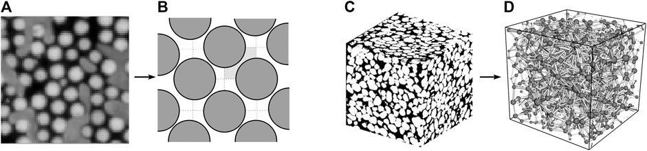
FIGURE 1. An overview of the network representation of two and three dimensional porous media. Figure (A) shows a $10\text{mm}\times 10\text{mm}$ crop of a $42\text{cm}\times 85\text{cm}$ Hele-Shaw cell, filled randomly with a monolayer of $1\text{mm}$-diameter glass beads, indicated by the white circles [50]. The black and gray colors in the image show the wetting and non-wetting fluids. Such a system can be modeled by a two-dimensional network of hour-glass shaped links as shown in (B), where the distribution in link radii and node positions can be tuned according to the system properties. In (B), the dark gray circles represent the beads and white represents the pores. The links are separated by dotted lines and the intersection of two such lines defines the position of a node. One link is colored by light gray. We like to point out that, (B) is not an exact reconstruction of the image shown in (A), rather it is a simplified illustration. In (C), we show a three dimensional Micro CT image of sand-pack (sample F42A in [51]) and the corresponding reconstructed pore network is shown in (D).

In network representation, a pore is typically consists of two wider pore bodies that are connected by a narrower pore throat as shown in Figure 2A. In our modeling approach, we assign the total pore space to a composite link and the nodes do not contain any volume. The centers of the pore bodies correspond to the positions of nodes. This introduces a variation in the cross-sectional area along the length of the link which is modeled by a simplified hourglass shape as shown in Figure 2B. The interfacial pressure ($p_c$) therefore depends on the position of the meniscus as it moves along the link. The functional dependence of $p_c$ on the position, obtained from Young-Laplace equation, takes the form [58],

$\left|p_c\left(x_k\right)\right|=\frac{2\gamma \cos \theta }{r_j}\left[1-\cos \left(\frac{2\pi x_k}{l_j}\right)\right](2)$

where $r_j$ is the average radius of a link j and $x_k\in [0,l_j]$ is the position of the kth meniscus inside the link. Here γ is the surface tension and θ is the contact angle between the meniscus and the pore wall. If $p_a$ and $p_b$ are the local pressures at the two nodes a and b across the link, the instantaneous local flow rate $q_j$ inside the link from node a to b is proportional to the difference between the viscous pressure drop $\text{Δ}p$ ($=p_b-p_a$) across the link and the total capillary pressure drop due to all the menisci inside the link. This can be calculated by [59],

$q_j=-\frac{g_j}{l_j{\mu }_j}\left[\text{Δ}{p}_j-{\displaystyle \sum }_k{p}_c\left(x_k\right)\right](3)$

where the sum is over all the menisci inside the link j, taking into account the direction of the capillary forces. ${\mu }_j$ is the saturation-weighted viscosity of the fluids present inside the link at that instant, given by ${\mu }_j=s_{j,\text{n}}{\mu }_{\text{n}}+s_{j,\text{w}}{\mu }_{\text{w}}$. Here $s_{j,\text{n}}=l_{j,\text{n}}/l_j$ and $s_{j,\text{w}}=l_{j,\text{w}}/l_j$ are the fractions of the link length occupied by the non-wetting and wetting fluids respectively, so that $s_{j,\text{n}}+s_{j,\text{w}}=1$. The term $g_j$ is the mobility of the link that depends on the cross section. We model piston-like creep flow at low Reynolds number without any film flow and different cross-sectional shapes can therefore be taken into account by this mobility term $g_j$. For the regular network in 2D we chose the links to be cylindrical with circular cross section for which $g_j=a_j{r}_j^2/8$ for Hagen-Poiseuille flow [1], where $a_j=\pi r_j^2$ is the cross-sectional area. In the reconstructed 3D network, the pores are triangular in shape that is characterized by a shape factor (G) defined as the ratio between the effective cross-sectional area of the pore and the square of its circumference. The effective cross-sectional areas of each of the three pore parts, the two wider pore bodies at the ends and the narrow throat in the middle, are calculated from the relation $\alpha ={\rho }^2/\left(4G\right)$, where ρ is the radius of the inscribed circle in that pore part [60]. The mobility contribution from each part of the pore is then obtained from the relation $g=3{\rho }^2\alpha /20$ [61, 62] and the mobility term $g_j$ for the total link is then calculated from the harmonic average of the contribution from the three individual terms given by,

$\frac{l_j}{g_j}=\frac{{\lambda }_1}{g_1}+\frac{{\lambda }_2}{g_2}+\frac{{\lambda }_3}{g_3}(4)$

where ${\lambda }_{\mathrm{1,2,3}}$ and $g_{\mathrm{1,2,3}}$ are the lengths and mobilities of the pore parts respectively as shown in Figure 2A.

FIGURE 2

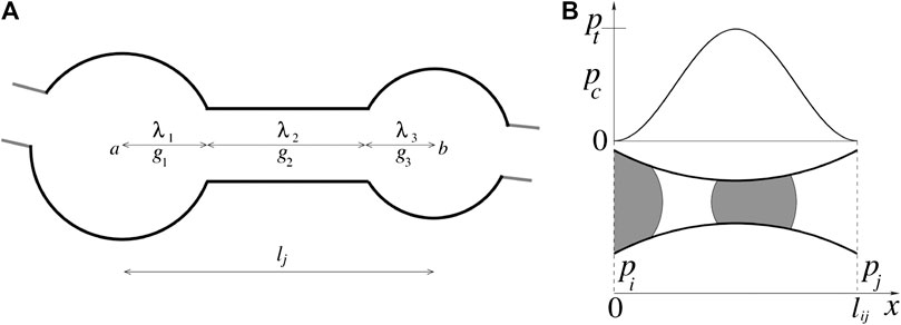
FIGURE 2. (A) Schematics of one pore in a reconstructed network which consists of three pore parts, two wider pore bodies at the ends and a narrow pore throat in the middle. ${\lambda }_{\mathrm{1,2,3}}$ and $g_{\mathrm{1,2,3}}$ are the lengths and mobility contributions from these three parts. The total length of the link is given by $l_j={\lambda }_1+{\lambda }_2+{\lambda }_3$ and the total mobility of the link is obtained from Eq. 4. This total pore space is modeled by an hour-glass shaped link as shown in (B) where the wetting and non-wetting fluids are colored by white and gray respectively. The variation in the interfacial pressure ($p_c$) due to this shape is modeled by Eq. 2 as shown above. Here $p_c$ is modeled by a cosine function, however one may consider some other functional form with a maximum in the middle that corresponds to the minimum of the pore radii at the narrow pore throat.

In order to move the fluids through the pores, the local pressures at nodes are needed to be solved at each time step. With the Kirchhoff equations, the net volume flux ($f_i$) through every node at each time step will be zero, that is, any node i,

$f_i={\displaystyle \sum _h{q}_h}=0,(5)$

where the subscript h runs over the links connected to the node i. This sum, along with Eqs. 2, 3, constructs a set of linear equations. We solve these equations with conjugate gradient solver [63] or the Cholesky factorization method [64] and the solutions of which at any time step provides the local node pressures $p_i$ at that step. The system can be driven by a constant global pressure drop $\text{Δ}P$ or a total flow rate Q with open or periodic boundary conditions. More details about implementing different boundary conditions will be presented in Section 4.

3 Meniscus-Dynamics Algorithms

After the fluid velocities inside all the links are known from the solution of Eq. 3, the next step is to displace the two fluids inside the links and to distribute them to the next links after they mix at the nodes. These are done by updating the meniscus positions between the two fluids at every time step. In our implementation, the full algorithm for the meniscus displacements is sub-divided into three intermediate functions, namely the (a) meniscus_move, (b) meniscus_create and (c) meniscus_merge, which are applied to each link and/or node at every time step. The meniscus_move function makes lateral displacements of the menisci in proportional to the fluid velocities in the respective links and calculates the amount of fluids that exit from each link to the connected node. The meniscus_create function then distribute these fluids from each node to the connected links with outward flow. The total pore space in our model is assigned to the composite links of the network where the competition between the viscous and capillary forces at any time step is taken care by Eq. 3. The nodes in our system do not contain any physical volume and this distribution of fluids from node to links is only an intermediate step. We therefore considered this distribution rule to be democratic, that is, it does not treat the two fluids differently. The volumes of the two fluids distributed to the links are therefore proportional to the ratio of the velocities in the outward links and to the ratio of the incoming volumes. These democratic rules are also possible to apply without any further change for a mixed wet system where wettability varies from pore to pore [65, 66], as all the changes in the contact angles can be accounted by Eq. 3 and no change in the meniscus algorithms are necessary. These two functions interpret the volume conservations of the two fluids together with the Kirchhoff laws. Finally, the third function meniscus_merge is used to merge bubbles inside any link and it limits the maximum number of menisci ($N_{\text{max}}$). This function is necessary as when fluids enter in the links from the nodes, new menisci are created at the entrance of the links which can make the meniscus number to increase indefinitely during the time stepping. In a real system, coalescence of bubbles occur inside the pores which limits the number of menisci. There are experimental studies to investigate the formation of bubbles and to find their characteristic size during flow through pore junctions [67], however, to our knowledge, there is no clear information available on the functional dependency of the maximum number of menisci or bubbles on the pore geometry and aspect ratio as well as on other flow parameters such as the fluid velocity, contact angle and surface tension. In order to get a detailed arrangement of fluids inside a pore, one needs to solve the flow equations at a much smaller scale, such as in Lattice Boltzmann simulations. In pore-network modeling, we are interested in the large-scale flow properties and not in the detailed configurations of fluids inside a pore. We therefore kept this number ($N_{\text{max}}$) as a tuning parameter in our algorithm which may be calibrated based on experimental observations. We constructed a merging algorithm that keeps the center of mass of the bubbles unchanged so that the overall fluid displacement does not get affected by the merging. We have performed a set of sensitivity test on the maximum meniscus number which we will present in Section 3.3.

In the following we present with all the technical details how these three functions can be implemented in any pore network. They are illustrated in Figure 3. We will verify a few identities in order to check whether they introduce any unphysical effect on fundamental flow properties.

FIGURE 3

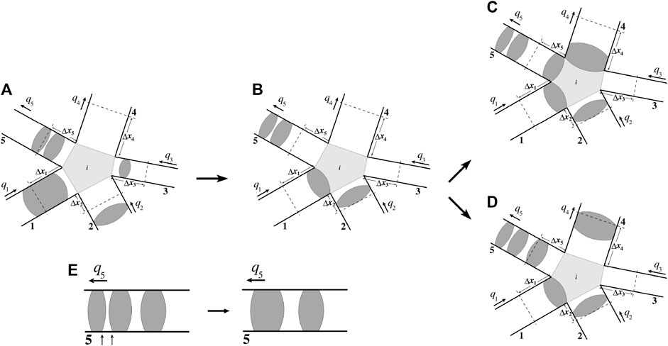
FIGURE 3. The three intermediate steps for the meniscus dynamics, the meniscus_move, meniscus_create and meniscus_merge, at every time step are illustrated here. Here five links, numbered as $j=1$, 2, 3, 4 and 5, are connected to the node i. However the above illustrations are also valid for any number of links. Wetting and non-wetting fluids inside the links are colored by white and dark gray respectively. All of the pore space are distributed to the links in this model and the area around the node i, colored by light gray, does not contain any real volume. (A) shows an example configuration of two fluids at a time step. Solution of the Kirchhoff equations as described in Section 2 provides the local flow rates $q_j$. Based on the directions of $q_j$ at this time step, say the links 1, 2 and 3 are identified as the incoming links whereas 4 and 5 are identified as the outgoing links here. Values of the displacements $\text{Δ}{x}_j$ for each link, calculated from $\text{Δ}{x}_j=q_j\text{Δ}t/a_j$ (see text) are shown by dashed lines. Every meniscus in a link j are moved toward (in the incoming links) or away from (in the outgoing links) the node by a distance $\text{Δ}{x}_j$ which is shown in (B). This is performed by the function meniscus_move. The total volume of the fluids ($a_1\mathit{\Delta }{x}_1+a_2\mathit{\Delta }{x}_2+a_3\mathit{\Delta }{x}_3$) which left the links 1, 2 and 3 into the node i is now to be placed at the beginning of the links 4 and 5, which will fill the volume $(a_4\mathit{\Delta }{x}_4+a_5\mathit{\Delta }{x}_5)$ and will create new menisci in the outgoing links as described in meniscus_create. There are two different ways of creating the new menisci, one is to place the wetting fluid first and the non-wetting next as shown in (C), and the other is to place the non-wetting fluid first and the wetting next as shown in (D). We adopt (C) and (D) alternatively at each consecutive time steps. (E) shows the meniscus_merge function for the link 5 when there are four allowed menisci. There link 5 has total six menisci before merging and the two bubbles around the two nearest menisci marked by the arrows are merged. The merging process are illustrated in more detail in Figure 4.

3.1 meniscus_move

The pore network consists of $N_{\text{L}}$ number of links that are connected to each other by $N_{\text{N}}$ number of nodes. We will use the subscript i for a node ($i=1,\dots ,N_{\text{N}}$) and the subscript j for a link ($j=1,\dots ,N_{\text{L}}$). The meniscus number inside a link is denoted by k. Inside the code, one also needs to mark the type of the menisci, for example, whether it is a meniscus at the beginning of a non-wetting bubble or at the end. This is necessary in order to calculate the direction of the capillary forces and also to measure the amount of two individual fluids that enter from a link to a node. Whether it is a regular network with constant coordination number for each node or an irregular network where the nodes have different coordination numbers, such as a reconstructed network from a real sample, it does not change any of the rules described in the following. In Figure 3, we illustrate them for an example of five links connected to a node i. At a time step, when all the pressures ($p_i$) at the nodes for an existing fluid configuration are known from the solutions of Kirchhoff equations, the flow rates $q_j$ inside the links are obtained from Eq. 3. A time interval ($\text{Δ}t$) is then decided in such a way that a meniscus inside any link does not move more than $10\text{\%}$ of corresponding link length at that time step. In order to do so, the link-velocities $c_j$ are calculated from local flow rates $q_j$ by $c_j=q_j/a_j$, where $a_j$ is the cross-sectional area of the link j. The time step is then calculated as

$\text{Δ}t=\frac{0.1l_j}{c_{j,\text{max}}},(6)$

where $c_{j,\text{max}}$ is the largest fluid velocity among all the links and $l_j$ is the length of that link. For the time evolution, we use an explicit Euler-type procedure. This works well for a large range of capillary numbers with only the time step criterion mentioned in Eq. 6. In order to ensure numerical stability at low capillary numbers, however, the sensitivity of interfacial pressure jumps to perturbations in meniscus positions must also be taken into account when choosing the time step, see [68]. This puts a limit on the maximum time step size that is independent of flow rate and thus becomes a severe criterion when flow rates are low. In [68] computational efficiency was improved at low capillary numbers by a semi-implicit method for a different type of meniscus algorithms. Here, however, we consider only capillary numbers that are large enough for Eq. 6 to be sufficient to ensure numerical stability. We will show some simulation results in Section 5.1 for $\text{Ca}={10}^{-5}$ and in our tests, we could run simulations at capillary numbers as low as $\text{Ca}={10}^{-6}$, though the simulations were highly time consuming. Simulations with capillary numbers lower than that are not doable within reasonable computational time.

After deciding the time step, menisci inside each link j are to be moved in the direction of $q_j$ by a distance,

$\text{Δ}{x}_j=c_j\text{Δ}t(7)$

as shown in Figures 3A,B. Here, the links have uniform cross-sectional area in terms of the mobility, so all the menisci inside the same link move by the same distance. The positions of all the menisci inside any link ($x_{j,k}$) are then updated, $x_{j,k}=x_{j,k}+\text{Δ}{x}_j$. By doing this, if any of the menisci moves outside any link ($x_{j,k}>l_j$), it is deleted from the list of menisci. The set of $p_i$s at the nodes decide which links, among all the links connected to a node, have fluids that flow toward the node and have fluids that flow away from the node at that time step. We name these links respectively as the incoming links and the outgoing links for that node. In the example shown in Figure 3 the links 1, 2 and 3 are the incoming links and the links 4 and 5 are the outgoing links for the node i at that time step. Due to the displacement of the menisci by an amount $\text{Δ}{x}_j$, a node i receives a certain volume (${\varphi }_{i,j}$) of wetting and/or non-wetting fluids from an incoming link j, given by ${\varphi }_{i,j}=a_j\text{Δ}{x}_j=q_j\text{Δ}t$ that leaves from the end of an incoming link j. The total volume of fluids ($V_i$) received by a node i from all of its incoming links is therefore,

$V_i={\displaystyle \sum _{j\in I}{\varphi }_{i,j}}=V_i^{\mathrm{w}}+V_i^{\mathrm{n}},(8)$

where $V_i^{\text{w}}$ and $V_i^{\text{n}}$ respectively are the total volume of wetting and non-wetting fluids arrived from all the incoming links to the node i. Here $j\in \text{I}$ denotes the set of all the incoming links connected to i. We point out that, in order to apply this meniscus_move function for the whole network, one can loop through all links j, move the menisci by the distance $\text{Δ}{x}_j$ and add up the amount of fluids that exit from the link to the connected node in the direction of the link-flow. This will produce the arrays of $V_i^{\text{w}}$ and $V_i^{\text{n}}$ at the end of the loop which will contain the incoming volume flux at each of the nodes at that time step. The marking of the meniscus types, as mentioned before, will allow here to calculate the individual terms $V_i^{\text{w}}$ and $V_i^{\text{n}}$. This is illustrated in Figure 3.

3.2 meniscus_create

After the function meniscus_move is performed over all the links, the list of the volumes $V_i^{\text{w}}$ and $V_i^{\text{n}}$ of incoming fluids for all the nodes are generated for that time step. As all of the pore space in this model is assigned to the links of the network and the nodes do not contain any physical volume, the total volume of incoming fluids ($V_i$) to a node are to be injected at the beginning of the outgoing links at the same time step. This will create new bubbles and menisci at the beginning of the outgoing links. The total volume of fluids that will enter from a node i to an outgoing link j is given by, ${\varphi }_{i,j}=q_j\text{Δ}t$, and due to the balancing of the Kirchhoff equations it ensures that ${\displaystyle {\sum }_{j\in I}{\varphi }_{i,j}}={\displaystyle {\sum }_{j\in O}{\varphi }_{i,j}}$ where $j\in \text{I}$ and $j\in \text{O}$ respectively denote the set of all incoming and outgoing links for the node i. However, we still need to find out the volumes of each individual fluid for any outgoing link, that is, how much of the wetting (${\varphi }_{i,j}^{\text{w}}$) and the non-wetting (${\varphi }_{i,j}^{\text{n}}$) volumes will enter into j. As illustrated in Section 3, we adopt a “democratic” rule to calculate this, that means both the wetting and non-wetting fluids get the same preference and the volumes depend on the flow rates $q_j$ of the respective outgoing links. For any outgoing link j, ${\varphi }_{i,j}^{\text{w}}$ and ${\varphi }_{i,j}^{\text{n}}$ are therefore calculated as,

${\varphi }_{i,j}^{\text{w}}=q_j{V}_i^{\text{w}}\text{Δ}t/V_i\text{and}{\varphi }_{i,j}^{\text{n}}=q_j{V}_i^{\text{n}}\text{Δ}t/V_i(9)$

which imply that the ratio of the volumes of a fluid among all the outgoing links are the same as the ratio between flow rates among those links. Distributing the fluids in this way also preserves the volume conservation of each individual fluid, that is,

${\displaystyle \sum _{j\in \text{O}}{\varphi }_{i,j}^{\text{w}}}=V_i^{\text{w}}\text{and}{\displaystyle \sum _{j\in \text{O}}{\varphi }_{i,j}^{\text{n}}}=V_i^{\text{n}}.(10)$

In each link, the wetting and non-wetting bubbles can be placed in two different ways, the non-wetting fluid at the beginning and the wetting fluid at the next, as shown in Figure 3C or in the other way as shown in Figure 3D. Here we adopt C or D alternatively at every consecutive time steps. One can also chose C or D randomly at every time step. This is equivalent of assuming that at some time step the wetting fluid coming from the incoming nodes pass the node before the non-wetting fluid enters the node, and the situation is the opposite in the other case.

As we mentioned before, the competition between the viscous and capillary forces only appear in Eq. 3 in our model. The meniscus displacement algorithms are therefore democratic and do not treat the wetting and the non-wetting fluids differently. This means, when the surface tension is set to zero, the capillary forces disappear and one will obtain [69],

$Q_{\text{w}}\left(S_{\text{w}},M\right)=Q_{\text{n}}\left(1-S_{\text{w}},1/M\right)(11)$

where $Q_{\text{n}}$ and $S_{\text{n}}$ are the total non-wetting flow rate and the non-wetting saturation. If we further set ${\mu }_{\text{w}}={\mu }_{\text{n}}$ when the surface tension is zero, the two fluids essentially become identical which will flow with equal velocity. This leads to,

$F_{\text{n}}=S_{\text{n}}(12)$

where, $F_{\text{n}}=Q_{\text{n}}/Q$, the non-wetting fractional flow in the steady state. These conditions can be used as preliminary tests for the meniscus functions whether they are implemented properly in the code. The precise way to measure the fractional flow and other measurable quantities will be presented in Section 5.

3.3 meniscus_merge

After the two functions meniscus_move and meniscus_create are executed for each link, we look for any link in which the number of menisci exceeds the maximum number $N_{\text{max}}$. Notice that, restricting the number of menisci inside a link does not necessarily impose any restriction on the minimum or maximum size of a bubble. In order to find out the best possible algorithm and to test its sensitivity, we performed numerical simulations with a network of $64\times 64$ links forming a diamond lattice in 2D with disorder in the link radii. We start with a simple merging rule A (merge_back), where we identified two nearest non-wetting bubbles inside a link. Among these two non-wetting bubbles, only one, say the one in the front toward the flow direction, is moved back toward the other bubble and then merged. The length of this merged non-wetting bubble is the sum of the two bubbles before merging which maintains the volume conservation. This reduces the meniscus count by two inside the link and the meniscus positions are updated accordingly. This is illustrated in Figure 4A. However, when we measure the non-wetting fractional flow for zero surface tension with equal viscosities of the fluids, that is for two identical fluids, we find a deviation from Eq. 12. This is shown in Figure 5A where a small but systematic deviation from the diagonal $F_{\text{n}}=S_{\text{n}}$ line can be observed which is unphysical. This effect is a consequence of displacing the non-wetting bubble opposite to the flow which introduces a decrease in the non-wetting fractional flow. We then tried the next rule B (merge_cm), where instead of merging two nearest non-wetting bubbles, we identified any two nearest menisci and merge the two bubbles across them. With this process, both the non-wetting or wetting bubbles can be merged whichever are the nearest. Moreover, instead of moving only one bubble toward the other, here we moved both the bubbles toward each other by such a distance so that the center of mass of these two bubbles does not change after merging. We illustrate this in Figure 4B. This rule shows satisfactory $F_{\text{n}}=S_{\text{n}}$ behavior at the zero capillary pressure as shown in Figure 5B. We then measured $F_{\text{n}}$ at finite capillary numbers $\text{Ca}=0.1$ and 0.01, and check the sensitivity and the qualitative behavior of the results. They are shown in the top row of Figure 6 for maximum bubble counts $N_{\text{max}}=2$ and 3. The $F_{\text{n}}$ vs. $S_{\text{n}}$ plot generally shows an S-shaped behavior for finite Ca in experiments and simulations [70, 71]. There are capillary barriers associated with the narrow pore throats which the fluids need to overcome. Consequently, the fluids flow with different velocities and the phase with larger volume fraction wins. The non-wetting fractional flow curve therefore stays under the diagonal for lower non-wetting saturation and above the diagonal for higher non-wetting saturation. Due to the direction of capillary forces between the wetting and non-wetting phases, the curves do not cross the diagonal at the middle. This makes fractional flow curve S-shaped when plotted against the saturation. When the saturation of a fluid is very high, it percolates through the system by trapping the other fluid in small clusters and the fractional flow of the percolating fluid become close to 1. However, for the merging scheme merge_cm (B), we see that the curve deviates from a typical S-shape and approaches to the diagonal line at higher saturation values ($S_{\text{n}}>0.8$). This seems an artificial effect introduced by the merging scheme B. It seems that, as we moved both the bubbles toward each other while merging, small bubbles connected to different links at the nodes got disconnected and started flowing. Moreover, the results also seem to be sensitive on the meniscus count. We therefore updated the merging scheme further on. In the third and final rule C (merge_cmnn), we added one additional criteria compared to B. There we made sure that any fluid bubble that is in contact to a node, does not get disconnected from the node during the merging process. In order to do so, if one of the two nearest bubbles are connected to a node, we did not move that bubble during the merging process and only moved the other one. Everything else in this rule C are the same as rule B. With this merging scheme, we found exact match of fractional flow with Eq. 12 at zero surface tension and also obtained the expected qualitative behavior for non-zero capillary pressure. These are shown in Figure 5C and in the bottom row of Figure 6 respectively. Moreover, while changing the maximum bubble count with this merging scheme, we find no noticeable difference in the qualitative behavior of $F_{\text{n}}$ with the change in $N_{\text{max}}$. This is shown in Figure 7 for $N_{\text{max}}=2$, 3, 4 and 5. We therefore finally adopt the merge_cmnn as the merging scheme.

FIGURE 4

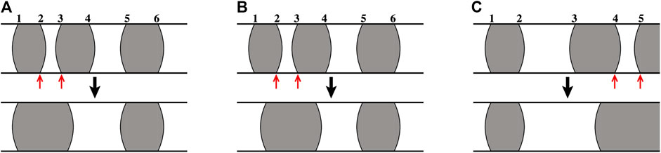
FIGURE 4. Illustration of the meniscus_merge function for maximum meniscus count $N_{\text{max}}=4$. The top row shows the meniscus positions before merging and the bottom row shows after merging. White and gray represent the two fluids inside the links. The nearest two menisci are indicated by red arrows. In (A) we show the simplest possible try, namely the merge_back scheme. The link had six menisci before merging among which the menisci 2 and 3 are the nearest. We merge them by moving only one bubble toward the other, so the meniscus 1 does not change its position, only the meniscus 4 is moved toward 1 by a distance that is equal to the distance between 2 and 3. In (B) we show the next possible try, namely the merge_cm. Here instead of moving the meniscus 4 toward 1, we move both 1 and 4 toward each other by such distances so that the center of mass of the two bubbles do not change after merging. The third and final meniscus merging scheme is merge_cmnn, which is same as (B) with an additional criteria as illustrated in (C). In the situation when one of the two nearest bubbles is connected to a node, such as the non-wetting bubble connected to the meniscus 5 in (C), it will get disconnected from the node according to the merging scheme (B). We avoid this disconnection of any bubble from a node by moving only the other bubble in such a situation as shown in (C). So to merge the nearest menisci 4 and 5, we only move the meniscus 3 toward the node. The merge_cmnn scheme is therefore a combination of (B) and (C) which we adopt here.

FIGURE 5

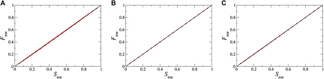
FIGURE 5. Plot of steady-state non-wetting fractional flow F_n as a function of non-wetting saturation S_n for zero capillary pressure at the menisci. The three plots correspond to the three merging schemes (A) merge_back, (B) merge_cm and (C) merge_cmnn as described in Section 3.3. A small but systematic deviation from the diagonal F_n = S_n line can be observed for A.

FIGURE 6

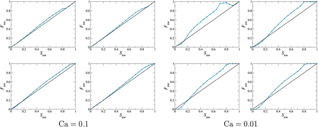
FIGURE 6. Steady-state fractional flow at finite capillary numbers $\text{Ca}=0.1$ and 0.01 with the merging rules B: merge_cm (top row) and C: merge_cmnn (bottom row). The left and right plots for each capillary number correspond to $N_{\text{max}}=2$ and 3 respectively. With B, $F_{\text{n}}$ approaches toward the diagonal line at higher saturation $S_{\text{n}}>0.8$ for the first three plots.

FIGURE 7

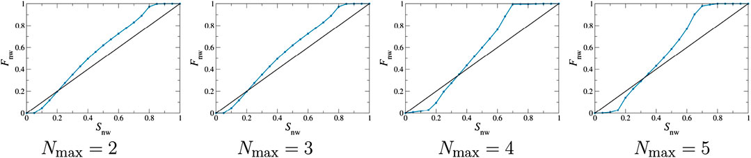
FIGURE 7. We show the effect of changing the maximum number of menisci (N_max) with the merging scheme C, the merge_cmnn. The steady‐state non-wetting fractional flow is plotted as a function of non-wetting saturation for N_max= 2, 3, 4 and 5. With such a change in the meniscus count, no noticeable difference is observed in the qualitative behavior in F_n.

4 Boundary Conditions

Simulations of different types of flow need proper boundary conditions to be implemented. The drainage displacement simulations can be performed with open boundary conditions (OB) where two opposite edges can be used as the inlets and outlets and the other edges are kept closed. Depending on the setup, all or some of the nodes and links at the inlet edge can be considered to inject a fluid. Depending on whether the system is driven under constant pressure drop or constant flow rate, either the node pressures ($p_i$) or the link flow rates ($q_j$) at the inlets are to be set externally. We also need to set the node fluxes ($V_i^{\text{w}}$ and $V_i^{\text{n}}$) at the inlets depending upon the type of fluid injected. For the injection of non-wetting fluid, all the $V_i^{\text{n}}$s are set to be one and the $V_i^{\text{w}}$s are set to be zero for all the inlet nodes. With these, we solve the equations for pressures and flow rates for all the other nodes and links inside the network.

The open boundary conditions can also be used for steady-state flow for the setup that is generally used in laboratory experiments [12]. There, instead of injecting one fluid, two fluids are injected simultaneously through alternate inlets. For this setup, all we need to do is to set the inlet node fluxes accordingly, all the $V_i^{\text{n}}$s are set to one for the non-wetting inlets and all the $V_i^{\text{w}}$s are set to one for the wetting inlets. The inlet flow rates define the total flow rate (Q) and the fractional flow $F_{\text{n}}=Q_{\text{n}}/\left(Q_{\text{n}}+Q_{\text{w}}\right)$. Here, $Q_{\text{n}}={\displaystyle {\sum }_{\text{n}}^{\prime }{q}_j}$ and $Q_{\text{w}}={\displaystyle {\sum }_{\text{w}}^{\prime }{q}_j}$ where ${\Sigma }_{\text{n}}^{\prime }$ and ${\Sigma }_{\text{w}}^{\prime }$ indicate the sum over all non-wetting and wetting inlets respectively. The fractional flow $F_{\text{n}}$ is an external parameter in this setup and the saturation $S_{\text{n}}$ is decided by the system.

Another way to simulate the steady-state flow is by implementing periodic boundary (PB) conditions in the direction of overall flow, which is generally not possible in the experiments. In the open boundary setup, the injection of two fluids via alternate inlets in the experiments creates boundary effects and makes spatially homogeneous steady-state regime smaller. With the periodic boundaries, such boundary effects can be avoided and relatively smaller systems may be used for similar statistics. For this, the inlet and outlet edges are connected so that the fluids leaving at the outlets, enter the system again through the inlets. The links that connect the inlets and outlets are called as the ghost links. The network therefore becomes a closed system and the two fluids keep flowing through the system. The saturation $S_{\text{n}}$ therefore is a control parameter here and the fractional flow is decided by the system. This is illustrated in Figure 8 for 2D and 3D networks. In case of 2D, periodic boundary conditions are applied in both directions which makes the flow equivalent to the flow on the surface of a torus as shown in B. For the reconstructed network in 3D, the opposite inlet and outlet edges are not identical. Therefore, to apply to periodic boundary conditions to this network we double the system by a mirror copy of the network in the direction of the flow, as shown by the two cuboids in D. This makes the inlets and outlets at the opposite edges identical, which we then connect with the ghost links to make the system periodic. With the periodic boundary, the inlets are seen as the neighbors of the outlets for the meniscus-dynamics algorithms. Here, the global pressure drop $\text{Δ}P$ to drive the flow needs to be added with the node pressure drops across the ghost links while solving Eqs. 3, 5.

FIGURE 8

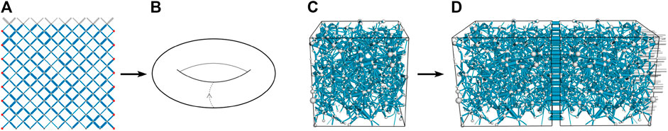
FIGURE 8. Implementation of periodic boundary conditions for 2D and 3D networks. A 2D regular network is shown in (A) where periodic boundary conditions are applied in both the directions. Here the overall flow is in the upward direction and the gray links at the top row represent the ghost links. The links are drawn as cylindrical tubes for the simplicity of drawing, but they are hourglass shaped in terms of the capillary pressure. The nodes are marked by small dots where the red dots at the left and right edges represent identical nodes. This makes the flow essentially on the surface of a torus as shown in (B) where the arrow represents the effective flow direction. For 3D, a network reconstructed from Beria sandstone is shown in (C) where the overall flow is from left to right. Periodic boundary conditions are applied in the direction of flow by adding a mirror copy of the the network as shown in (D). The ghost links at the right are colored by gray.

The structure of the complete simulation with all the meniscus dynamics functions is the following:

(1) Network: construct or read

(2) Define: boundary conditions

(3) Initialize: random or sequential fluid distribution

(4) for$t=1$ to $timesteps$do

(5)  Solve the pressure field

(6)  for$j=1$ to $totallinks$do

(7)   meniscus_move(j)

(8)  end for

(9)  for$j=1$ to $totallinks$do

(10)  meniscus_create(j)

(11)  meniscus_merge(j)

(12) end for

(13) Calculate measurable quantities at t

(14) end for

During initialization, the initial positions of all the menisci in each link need to be defined depending on the saturation and how we want to start the simulation. Then after solving the pressure field, the meniscus_move function is to be performed on all the links which will generate the array of the node fluxes $V_i^{\text{w}}$ and $V_i^{\text{n}}$ for each node i. These arrays will then be used as the input to the meniscus_create function which will create the new menisci in the links. The code for the first three steps in the above method will vary according to different requirements of the simulation.

5 Applications and Validation

As stated earlier, the meniscus algorithms in this pore-network model has the flexibility to be applied for different network topologies and boundary conditions. Moreover, we can study both the transient and the steady-state properties. In our simulations, we consider a network of links forming a tilted square lattice at an angle ${45}^{\circ }$ with the direction of applied pressure drop in 2D. The length of each link ($l_j$) is $1\text{mm}$ and their radii ($r_j$) are taken from a uniform distribution of random numbers in the range from $0.1\text{mm}$ to $0.4\text{mm}$. In 3D, we consider a network that is reconstructed from a real sample of Berea sandstone by using micro-CT scanning [49, 51]. The reconstructed network contains 2,274 links that are connected via 1,163 nodes and has a physical dimension of ${1.8}^3{\text{mm}}^3$. We doubled this network by adding a mirror image of itself in the direction of the applied pressure drop in order to apply periodic boundary conditions. In the following, we present some of the fundamental results of transient and steady-state of two-phase flow in porous media by using this pore-network model. All the following results are obtained only by changing the parameter values and the boundary conditions as necessary, while using the exactly same algorithms for meniscus displacements.

5.1 Drainage Displacements

As described in the introduction, when a non-wetting fluid is invaded into a porous medium filled with a wetting fluid, it generates different types of invading flow patterns depending on the capillary number and viscosity ratio. A less viscous fluid displacing a high viscous fluid creates viscous fingering patterns at a high Ca [6, 17] and capillary fingering patterns at low Ca [8]. The capillary and viscous fingering patterns resemble with the invasion percolation [7] and diffusion limited aggregation (DLA) models [9] respectively. Alternatively, when a high viscous fluid displaces a low viscous fluid, a stable displacement front is observed. In order to verify whether our pore-network model can reproduce these different flow patterns during the drainage, we run different simulations for different values of the capillary number $\text{Ca}$ and viscosity ratio M. In our simulations, we set $\gamma \cos \theta =0.03$ N/m. The results are highlighted in Figure 9. Here $M={\mu }_{\text{n}}/{\mu }_{\text{w}}$ where ${\mu }_{\text{n}}$ and ${\mu }_{\text{w}}$ are the viscosities of the invading blue non-wetting fluid and the defending gray wetting fluid. In the top row the low viscous non-wetting fluid displaces the more viscous fluid where one can observe the development of the viscous fingering pattern. In the second row $M={10}^2$, and a more viscous blue fluid is displacing the less viscous gray fluid and a compact and stable displacement front is observed [5]. Flow patterns in the third row correspond to capillary fingering which are generated with the simulations at a very low capillary number $\text{Ca}={10}^{-5}$. These fingering patterns are more fractal than the viscous fingering and depend strongly on the system disorder. For a more quantitative measurement of the different regimes, one can measure the fractal dimensions of the fingering patterns. We like to point out that, these three different transient regimes are generated only by altering the values of the flow rate Q and the viscosities of the two fluids to set the values of Ca and M, and no modification in the meniscus dynamics algorithms were made between different simulations.

FIGURE 9

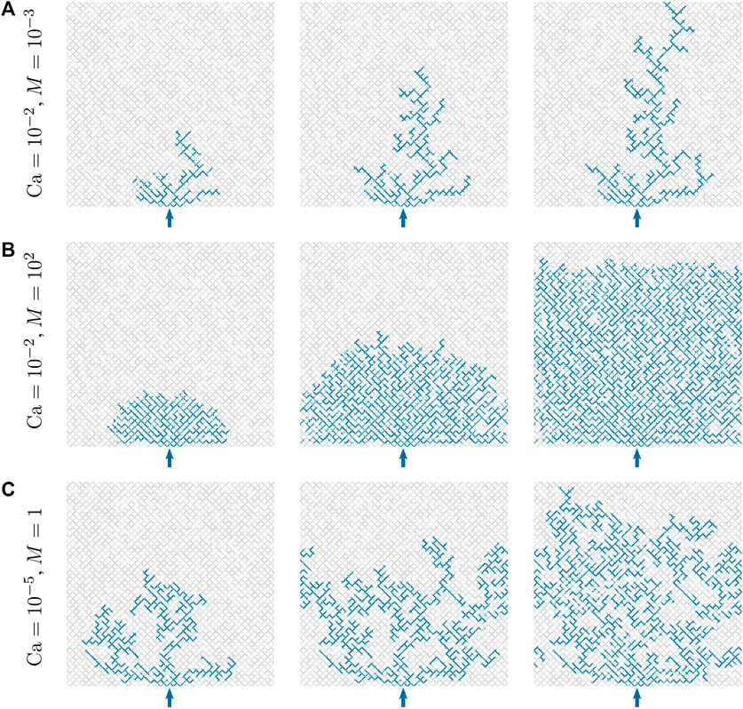
FIGURE 9. Development of transient flow patterns during the drainage simulations in a disordered square network of 64 × 64 links. The network is initially filled with wetting fluid (gray) and the non-wetting fluid (blue) is injected through four inlet nodes at the bottom edge of the network, shown by the arrow, with a constant flow rate. The top edge of the network is kept open which works as the outlet. Periodic boundary conditions are applied in the horizontal direction, therefore the left and right edges are connected together. Only the capillary number Ca and the viscosity ratio M are altered during these simulations and all other flow parameters and the algorithms for meniscus dynamics are exactly the same. The flow patterns show the different regimes of transient two-phase flow, namely (A) the viscous fingering (B) the stable displacement and (C) the capillary fingering. We like to point out that, though we adopted “democratic” rules for meniscus algorithms, it is the solution of the flow equations that lead the fluids to generate these different flow patterns.

5.2 Steady State

Steady-state flow can be simulated by implementing either open or periodic boundary conditions as shown in Figure 10. In the open boundary simulation shown in the first row, the wetting and non-wetting fluids are injected through alternate injection points at the bottom edge of the network. The top edge is kept open through which fluids leave the system. The two edges on the sides are connected through periodic boundary which can also be kept closed if necessary. The simulations are performed at constant fractional flow by setting the flow rates at the inlet links. Due to the traces of the injections near the inlet edge, a long enough system is necessary for the open boundary simulations to obtain a region of spatially homogeneous steady-state flow away from the inlets. The second row of Figure 10 shows simulation with periodic boundary conditions in both directions. Here the system is closed and the control parameter is the fluid saturation. In the third row, we show the simulation with a three dimensional reconstructed Berea network where the periodic boundary condition is applied in the direction of the overall flow. The total flow rate is controlled in these simulations and we measure the global pressure drop ($\text{Δ}P$). By plotting $\text{Δ}P$ as a function of the injected pore-volumes as shown in the right of each row, we identify the steady states, that is when $\text{Δ}P$ fluctuates around an average value.

FIGURE 10

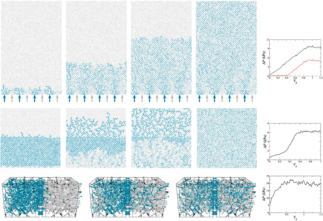
FIGURE 10. Steady-state simulations at $\text{Ca}=0.001$ and $M=1$ with different boundary conditions. The wetting and non-wetting fluids are colored by gray and blue. The top row shows simulation with open boundary at $F_{\text{w}}=0.5$ with a 2D diamond network of $64\times 100$ links. The next two rows respectively show simulations with periodic boundary for $S_{\text{w}}=0.5$ with a 2D network of $64\times 64$ links and with a 3D reconstructed network of Berea sandstone. The directions of the overall flow is from the bottom to top for 2D simulations and from the left to right for 3D simulations. For each system, the measured global pressure drops ($\text{Δ}P$) as a function of the pore volumes ($V_{\text{p}}$) of fluids passed are shown at the right where the red and black curves for the first system show the pressure drops at the middle and at the inlet of the system with respect to the outlet row.

In the following, we present two sets of simulation results with this dynamic pore network model to show the agreement with the steady-state properties of two-phase flow. First, we will present the effective rheological properties where the total flow rate shows non-linear dependence on the pressure drop in the capillary dominated regime [12–15]. Next, we will measure seepage velocities and will verify the relations between them [25]. We will also describe in detail how to measure the different quantities from the simulation, such as the flow rates and the seepage velocities of different fluid components.

Effective Rheology and Crossover from Linear to Non‐linear Flow Regime

When two Newtonian fluids flow through a porous media, it was found experimentally [11–13, 15], numerically [14, 15] and with mean field calculations [14] that, in the regime when capillary forces compete with the viscous forces, that is, in the low capillary number regime, the total flow rate Q in the steady state does not follow the linear Darcy relation and varies quadratically with the excess pressure drop. This can be written as,

$\begin{array}{cc}Q=0,& P\le P_t\\ \sim {\left(\Delta P-P_t\right)}^2,& P>P_t\end{array}(13)$

where ($P_t$) is a global yield threshold pressure ($P_t$) below which there is no flow through the system. Study also shows that the non-linear behavior depends on the distribution of the threshold pressures as well as on the system geometry [72]. This is related to the capillary pressures at the menisci that create threshold barriers at the pore throats. These pores start opening while increasing the pressure drop, which leads the total flow rate Q to increase faster than the increase in $\text{Δ}P$. At sufficiently high pressure drop, all the pores start flowing and there is a crossover to a linear regime.

In order to verify this non-linear rheological behavior with our model, we performed steady-state simulations with the 2D square network and the 3D Berea network. The details of the networks were described in Section 5. Simulations are performed at constant total flow rate Q and the average global pressure drop $\text{Δ}P$ is measured in the steady state. Here the steady-state was achieved by using periodic boundary conditions. For 2D, the data is averaged over 20 different samples. The results are presented in Figure 11 where we plot the overall flow rate Q as a function of ($\text{Δ}P-P_t$). The threshold pressures $P_t$ are calculated by plotting $\text{Δ}P$ vs. $\sqrt{Q}$ as shown in the insets. When the results follow Eq. 13, it will produce straight lines for the lower values of $\text{Δ}P$, where the intercepts of the straight lines at y-axis correspond to the values of $P_t$. The results show two distinct regimes, a quadratic regime with slope $\approx 2$ satisfying Eq. 13 at the low pressure drops and a linear regime with slope $\approx 1$ at high pressure drops. More simulation results on this non-linear rheological properties for different flow parameters and network geometries can be found in [15], where the meniscus algorithms were used for steady-state flow and the results were compared with experiments.

FIGURE 11

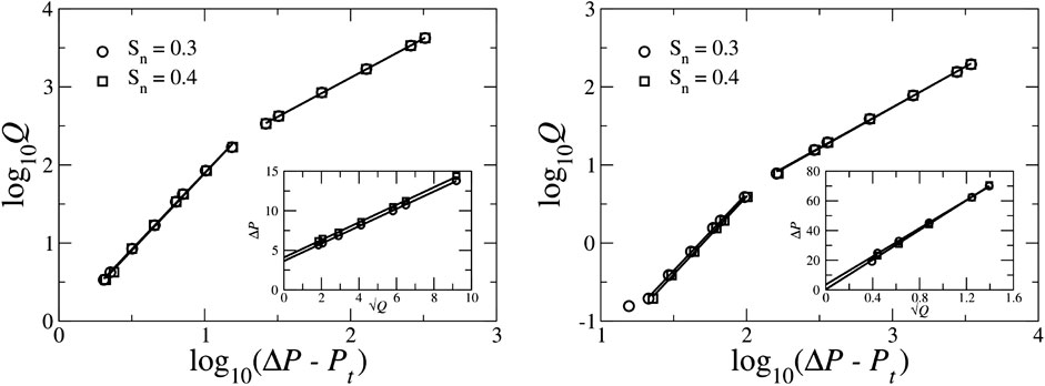
FIGURE 11. Variation of the total volumetric flow rate Q (${\text{mm}}^3/\text{s}$) with the overall pressure drop $\text{Δ}P$ (kPa) in the steady state for square and Berea networks. In the inset, $\text{Δ}P$ is plotted against $\sqrt{Q}$ for the low Ca regime where the intercepts at the y-axis correspond to the values of threshold pressures ($P_t$). For 2D, we find $P_t=3.65$kPa and 4.09 kPa for $S_{\text{n}}=0.3$ and 0.4 respectively. For the Berea network in 3D, we find $P_t=3.54$kPa and 0.32kPa for $S_{\text{n}}=0.3$ and 0.4 respectively. Using these values, we plot ${\text{log}}_{10}Q$ vs. ${\text{log}}_{10}\left(\text{Δ}P-P_t\right)$ which shows two distinct regimes at low and high pressures. For the linear regime, the slopes are obtained as $0.99\pm 0.01$ and $1.00\pm 0.01$ for 2D and $1.03\pm 0.01$ and $1.04\pm 0.01$ for 3D for the two saturations respectively. For the quadratic regime, the slopes are obtained as $1.96\pm 0.02$ and $1.98\pm 0.03$ for 2D and $1.98\pm 0.03$ and $1.99\pm 0.04$ for 3D.

Relation between Seepage Velocities

We will now measure the seepage velocities of the fluids in the steady state with this model and will verify the relations between them. When the system is driven under a constant pressure drop $\text{Δ}P$, a set of equations relating the wetting and non-wetting seepage velocities ($v_{\text{w}}$, $v_{\text{n}}$) to the total seepage velocity v and the fluid saturations can be derived using the Euler homogeneity property of the total flow rate Q in the steady state [25]. These relations necessitate a new velocity function, namely the co-moving velocity ($v_m$), which is a characteristic of the porous medium. The seepage velocities for the wetting and non-wetting fluids are defined as

$v_{\text{w}}=\frac{Q_{\text{w}}}{A_{\text{w}}}\text{and}{v}_{\text{n}}=\frac{Q_{\text{n}}}{A_{\text{n}}}(14)$

respectively, where $Q_{\text{w}}$ and $Q_{\text{n}}$ are the volumetric flow rates of the two fluids in the direction of the applied pressure drop. Quantitatively, $Q_{\text{w}}$ and $Q_{\text{n}}$ are defined as the volume of the wetting and non-wetting fluids that pass through any cross section of the system, perpendicular to the overall flow direction, per unit time. $A_{\text{w}}$ and $A_{\text{n}}$ are the wetting and non-wetting pore areas defined as the areas occupied by the wetting and non-wetting fluids along any orthogonal cross section through the system. This is illustrated in Figure 12 where $\text{Δ}P$ is applied in the positive x direction. The length of the systems in this direction is L. A cross section normal to the x direction is shown by an orange straight line for the 2D network and by an orange grid plane for the 3D network. Orthogonal views of these cross sections are shown underneath where the gray and blue patches show the pore areas occupied by the wetting and non-wetting fluids respectively. The sum of the areas of individual colors correspond to the wetting and non-wetting pore areas $A_{\text{w}}$ and $A_{\text{n}}$ along this cross section. For a homogeneous porous medium the average values of $A_{\text{w}}$ and $A_{\text{n}}$ remain same for any orthogonal cross section of the system in the steady state. Here we measure $A_{\text{w}}$ and $A_{\text{n}}$ by averaging the pore areas over all possible cross sections along x. The total pore area A related to all the fluids is therefore given by $A=A_{\text{w}}+A_{\text{n}}=\varphi A_s$ where ϕ is the porosity and $A_s$ is the average cross-sectional area of the total system including the pore space and the solid. With this, we can express the fluid saturations $S_{\text{w}}$ and $S_{\text{n}}$ in terms of the pore areas by $S_{\text{w},\text{n}}=V_{\text{w},\text{n}}/V_p=\left(A_{\text{w},\text{n}}L\right)/\left(AL\right)=A_{\text{w},\text{n}}/A$. The total flow rate Q of the two fluids is the sum of the wetting and non-wetting flow rates given by $Q=Q_{\text{w}}+Q_{\text{n}}=A_{\text{w}}{v}_{\text{w}}+A_{\text{n}}{v}_{\text{n}}$. Correspondingly, the total seepage velocity v associated with the total flow rate Q is defined by,

$v=\frac{Q}{A}(15)$

and we can find,

$v=S_{\text{w}}{v}_{\text{w}}+S_{\text{n}}{v}_{\text{n}}(16)$

by using the relations mentioned above.

FIGURE 12

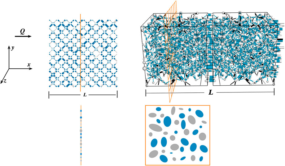
FIGURE 12. Description of the system to measure the flow rates (Q, $Q_{\text{w}}$, $Q_{\text{n}}$), the pore areas (A, $A_{\text{w}}$, $A_{\text{n}}$) and the seepage velocities (v, $v_{\text{w}}$, $v_{\text{n}}$) for the 2D and 3D networks. The global pressure drop $\text{Δ}P$ is applied in the x direction which is the direction of overall flow. A random cross section of the system normal to the direction of overall flow is shown by the orange line for 2D and by the orange grid plane for 3D. The normal view of the cross sections are shown underneath where the gray and blue patches show the occupation by wetting and non-wetting fluids in the cross section. The total gray and blue areas correspond to the wetting and non-wetting pore areas respectively and the sum of them correspond to the total pore area along this cross section. The averages of these areas over all the possible cross sections lead to the measurement of A, $A_{\text{w}}$ and $A_{\text{n}}$. In this figure, the gray and blue patches shown in the normal view of the cross sections do not reflect the actual occupations of the fluids in the above networks and are given as illustration purpose only.

In our network simulations, we have the information about the local flow rates $q_i$ and the meniscus positions for each link i at any time step. When the system is driven under constant pressure drop ($\text{Δ}P$), calculating the average flow rates and the pore areas along any orthogonal cross section of the network from the local flow rates are not straight forward, specially in case of an irregular network. For a regular network in 2D, all the links are of the same length $l_j=1\text{mm}$ and they are oriented along the same angle (${45}^{\circ }$) with respect to the overall flow direction. The sum of the local flow rates through each row of links normal to the flow direction is therefore the same for any row and the flow rates can therefore be measured by summing over all the links of the network and then dividing by the number of rows. This given by,

$Q=\frac{1}{N_L}{\displaystyle \sum _j{q}_j},Q_{\text{w}}=\frac{1}{N_L}{\displaystyle \sum _j{s}_{\text{w},j}{q}_j}\text{and}{Q}_{\text{n}}=\frac{1}{N_L}{\displaystyle \sum _j\left(1-s_{\text{w},j}\right)q_j}(17)$

where $N_L$ is the number of rows along L, i. e. 64 here. Similarly, we can calculate the cross-sectional areas as,

$A=\frac{1}{N_L}{\displaystyle \sum _j{a}_j},A_{\text{w}}=\frac{1}{N_L}{\displaystyle \sum _j{s}_{\text{w},j}{a}_j}\text{and}{A}_{\text{n}}=\frac{1}{N_L}{\displaystyle \sum _j\left(1-s_{\text{w},j}\right)a_j}(18)$

where $a_j$ is the cross-sectional area of the link j, projected into the plane normal to the flow direction. The wetting saturations of the links $s_{\text{w},j}$ are provided by the meniscus positions. Here the individual terms corresponding to the wetting and non-wetting phases are multiplied with the corresponding link saturations as the probability that a cross section through a link will pass through the wetting or non-wetting phase is proportional to the link saturation of that phase.

For an irregular network that is considered here in 3D, the links are of different lengths and oriented in different directions. In that case, measurement of the flow rates and the areas by summing over all the links and dividing by the number of rows using Eqs. 17, 18 will lead to wrong results. In this case, we measure these quantities in the following way. Let us consider an orthogonal cross-sectional plane at a random position through which we like to measure the flow rates (see Figure 12). The probability that any link j will pass through this plane will be proportional to $l_{x,j}/L$ where $l_{x,j}$ is the length of the link j in the x direction, the direction of the overall flow. After the link is selected, the probability that the plane will pass through the wetting fluid inside the link will be proportional to the local wetting saturation $s_{\text{w},j}$ of the link. Considering these probabilistic terms, the total flow rates Q, $Q_{\text{w}}$ and $Q_{\text{n}}$ through a random orthogonal cross section can therefore be calculated from the sum of the local flow rates over the links which pass through this cross section,

$Q=\frac{1}{L}{\displaystyle \sum _j{l}_{x,j}{q}_j},Q_{\text{w}}=\frac{1}{L}{\displaystyle \sum _j{l}_{x,j}{s}_{\text{w},j}{q}_j}\text{and}{Q}_{\text{n}}=\frac{1}{L}{\displaystyle \sum _j{l}_{x,j}\left(1-s_{\text{w},j}\right)q_j}(19)$

where L is the length of the network in the x direction. The areas can be measured in the similar way given by,

$A=\frac{1}{L}{\displaystyle \sum _j{l}_{x,j}{a}_j},A_{\text{w}}=\frac{1}{L}{\displaystyle \sum _j{l}_{x,j}{s}_{\text{w},j}{a}_j}\text{and}{A}_{\text{n}}=\frac{1}{L}{\displaystyle \sum _j{l}_{x,j}\left(1-s_{\text{w},j}\right)a_j}(20)$

For the regular 2D network, $l_{x,j}$ are the same for all the links ($=l$) and we recover Eqs 17, 18 by using $N_L=L/l$. After measuring the flow rates and the pore areas, the seepage velocities v, $v_{\text{w}}$ and $v_{\text{n}}$ are calculated using Eqs. 14, 15. Results are averaged over time in the steady state.

The calculation of v, $v_{\text{w}}$ and $v_{\text{n}}$ from the measurements of the flow rates and the pore areas should satisfy Eq. 16. In Figure 13 (top row), we plot $S_{\text{w}}{v}_{\text{w}}+S_{\text{n}}{v}_{\text{n}}$ against the total seepage velocity v where we used Eqs. 17, 18 for 2D and Eqs. 19, 20 for 3D. The plots show exact match of Eq. 16 for the whole range of parameters.

FIGURE 13

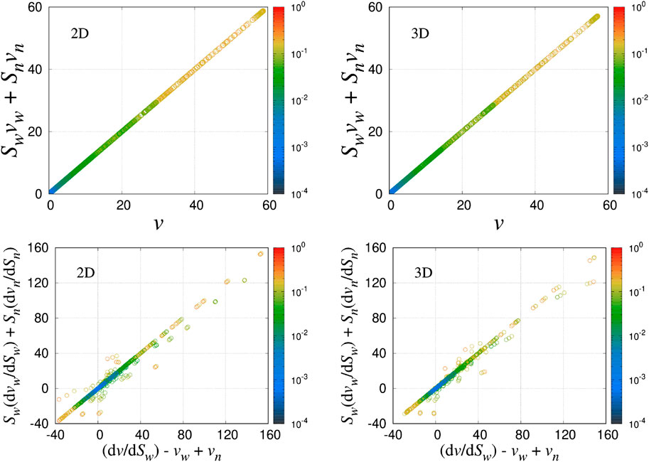
FIGURE 13. Plots of $S_{\text{w}}{v}_{\text{w}}+S_{\text{n}}{v}_{\text{n}}$ against the total seepage velocity v for 2D and 3D are shown in the top. The flow rates and pore areas to calculate $v_{\text{w}}$, $v_{\text{n}}$ and v are measured using Eqs. 17, 18 for 2D and using 19 and 20 for 3D. The velocities are in the unit of $\text{mm}/\text{s}$. The colors represent the capillary numbers which are in the range of $0.0007-0.2985$ for 2D and $0.001-0.271$ for 3D. The measurements show the exact match of Eq. 16 for both 2D and 3D. In the bottom, we plot the co-moving velocity $v_m$ calculated using Eq. 26, $v_m=S_{\text{w}}\left(\text{d}{v}_{\text{w}}/\text{d}{S}_{\text{w}}\right)+S_{\text{n}}\left(\text{d}{v}_{\text{n}}/\text{d}{S}_{\text{n}}\right)$ vs. the same using Eq. 25, $v_m=\left(\text{d}v/\text{d}{S}_{\text{w}}\right)-v_{\text{w}}+v_{\text{n}}$ for the square and Berea networks. The data shows good a agreement with Eqs. 26, 25 for the whole range of capillary numbers.

The total flow rate Q in the steady state is a homogeneous function of order one of the pore areas $A_{\text{w}}$ an $A_{\text{n}}$, that is, if we scale the three areas by $A\to \lambda A_{\text{w}}$, $A_{\text{n}}\to \lambda A_{\text{n}}$ and $A_s\to \lambda A_s$ by keeping the porosity ϕ constant, the volumetric flow rate Q scales as, $Q\left(\lambda A_{\text{w}},\lambda A_{\text{n}}\right)=\lambda Q\left(A_{\text{w}},A_{\text{n}}\right)$. This property of Q leads to a new set of equations between the seepage velocities. Complete derivations of the equations can be found in Ref. [25] and here we will present them in brief and will use them to validate our model. Taking the derivative of the homogeneity equation of Q with respect to λ and then setting $\lambda =1$ we get,

$v=S_{\text{w}}{\left(\frac{\partial Q}{\partial A_{\text{w}}}\right)}_{A_{\text{n}}}+S_{\text{n}}{\left(\frac{\partial Q}{\partial A_{\text{n}}}\right)}_{A_{\text{w}}}.(21)$

These two partial derivatives in the above equation have the units of velocity and correspondingly they define two thermodynamic velocities ${\widehat{v}}_{\text{w}}$ and ${\widehat{v}}_{\text{n}}$ given by,

${\widehat{v}}_{\text{w}}={\left(\frac{\partial Q}{\partial A_{\text{w}}}\right)}_{A_{\text{n}}}\text{and}{\widehat{v}}_{\text{n}}={\left(\frac{\partial Q}{\partial A_{\text{n}}}\right)}_{A_{\text{w}}}.(22)$

With these definitions Eq. 21 becomes,

$v=S_{\text{w}}{\widehat{v}}_{\text{w}}+S_{\text{n}}{\widehat{v}}_{\text{n}},(23)$

which has the similar form of Eq. 16. However, this does not imply that the thermodynamic velocities ${\widehat{v}}_{\text{w}}$ and ${\widehat{v}}_{\text{n}}$ are the same as the seepage velocities $v_{\text{w}}$ and $v_{\text{n}}$ that we measure. These two types of velocities can be related by a new velocity function is $v_m$ given by,

${\widehat{v}}_{\text{w}}=v_{\text{w}}+S_{\text{n}}{v}_m\text{and}{\widehat{v}}_{\text{n}}=v_{\text{n}}-S_{\text{w}}{v}_m(24)$

which fulfill both Eqs. 16, 23. This velocity function $v_m$ is a function of the saturation $S_{\text{w}}$ and called as the co-moving velocity, which is a property of the pore-network. With this definition of $v_m$, we can derive two equations that are related to the variation of saturation,

$\frac{\text{d}v}{\text{d}{S}_{\text{w}}}=v_{\text{w}}-v_{\text{n}}+v_m(25)$

and

$S_{\text{w}}\frac{\text{d}{v}_{\text{w}}}{\text{d}{S}_{\text{w}}}+\left(1-S_{\text{w}}\right)\frac{\text{d}{v}_{\text{n}}}{\text{d}{S}_{\text{n}}}=v_m.(26)$

In order to verify whether our pore-network model with the set of meniscus algorithms described here do satisfy these equations, we perform a large number of simulations with a wide range of parameters for the 2D square network and the 3D Berea network. Five viscosity ratios, $M=0.5$, 1, 2, 5 and 10 are considered where the wetting viscosity is chosen as ${\mu }_{\text{w}}=0.1\text{Pa}.\text{s}$. The non-wetting viscosity ${\mu }_{\text{n}}$ is then chosen accordingly in order to set the value of M. For each value of M, three different values of the surface tension, $\gamma =0.02$, 0.03 and $0.04\text{N}/\text{m}$, are considered. For each set of M and γ, we considered a set of pressure drops $\left|\Delta P/L\right|=0.16$, 0.20, 0.40, 0.80, 1.0 and $2.0\text{MPa}/\text{m}$ for 2D and 10, 20, 40, 80 and $160\text{MPa}/\text{m}$ for 3D. These values of pressure drops are chosen in order to get capillary numbers $\text{Ca}$ in a range around ${10}^{-3}$ to ${10}^{-1}$. Specifically, we find $\text{Ca}$ in the range of $0.0007-0.2985$ for 2D and $0.001-0.271$ for 3D. For any set of parameters, saturations are varied in the range of 0–1 in the steps of 0.05 which correspond to 21 saturation values. This led to a total of 1890 independent simulations for 2D and 1575 simulations for 3D in steady state.

The seepage velocities are measured for all the simulations and the derivatives with respect to the saturations are measured with central difference technique. We calculate the values of $v_m=\left(\text{d}v/\text{d}{S}_{\text{w}}\right)-v_{\text{w}}+v_{\text{n}}$ (Eq. 25) and $v_m=S_{\text{w}}\left(\text{d}{v}_{\text{w}}/\text{d}{S}_{\text{w}}\right)+S_{\text{n}}\left(\text{d}{v}_{\text{n}}/\text{d}{S}_{\text{n}}\right)$ (Eq. 26) and plot in Figure 13 (bottom row). The results show good agreement with Eqs. 25, 26 for both square and Berea networks for the whole range of the capillary numbers as indicated by the color scale. The few data points that are outside the straight line mostly correspond to the simulations near $S_{\text{w}}=0$ or 1 where the system undergoes from two-phase to single phase regime that creates a jump in the derivatives.

Eqs. 16, 26 transform the wetting and non-wetting velocities ($v_{\text{w}}$, $v_{\text{n}}$) to (v, $v_m$) while varying the saturation. By inverting the velocity transformation, it is possible to find equations to transform the total velocity and the co-moving velocity (v, $v_m$) to ($v_{\text{w}}$, $v_{\text{n}}$), which are given by,

$v_{\text{w}}=v+S_{\text{n}}\left(\frac{\text{d}v}{\text{d}{S}_{\text{w}}}-v_m\right)\text{and}{v}_{\text{n}}=v-S_{\text{w}}\left(\frac{\text{d}v}{\text{d}{S}_{\text{w}}}-v_m\right).(27)$

With these equations we can verify the measured values of wetting and non-wetting seepage velocities $v_{\text{w}}$ and $v_{\text{n}}$ against the ones calculated from these equation. In Figure 14, we plot $v+S_{\text{n}}\left(\text{d}v/\text{d}{S}_{\text{w}}-v_m\right)$ and $v-S_{\text{w}}\left(\text{d}v/\text{d}{S}_{\text{w}}-v_m\right)$ against the measured value of $v_{\text{w}}$ and $v_{\text{n}}$ respectively. While calculating $v_{\text{w}}$ and $v_m$ using above equations, we used the values of $v_m$ that are obtained from Eq. 26. For the whole range of the capillary numbers, good match with Eq. 27 can be observed for both the square and the Berea networks.

FIGURE 14

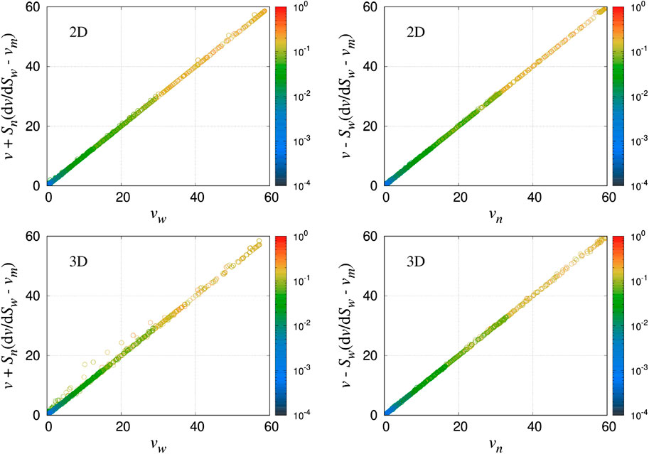
FIGURE 14. Plot of the wetting and non-wetting seepage velocities (mm/sec) calculated using Eq. 27 against the measured values of $v_{\text{w}}$ and $v_{\text{n}}$ for the square (top row) and Berea (bottom row) network. The derivatives are calculated using the central difference techniques. The color scale shows the capillary numbers.

Finally, we plot the co-moving velocity $v_m$ as a function of both $S_{\text{w}}$ and $\text{d}v/\text{d}{S}_{\text{w}}$ in Figure 15. Here $v_m$ was calculated using Eq. 25 in Figure 15. The data for $v_m$ roughly shows a planer form given by,

$v_m=a{S}_{\text{w}}+b\frac{\text{d}v}{\text{d}{S}_{\text{w}}}+c.(28)$

By fitting all the data points for the whole set of simulations, we find $a=-6.36\pm 0.25$, $b=0.94\pm 0.01$ and $c=5.00\pm 0.13$ for the square network and $a=-12.94\pm 0.62$, $b=0.88\pm 0.01$ and $c=10.10\pm 0.32$ for the Berea network. The planes using these parameters are shown in the respective figures with grid lines. The co-moving velocity is a property of the porous material and a function of the saturation $S_{\text{w}}$, total seepage velocity v and the variation of v while changing the saturation. Therefore it is not enough to specify only the $S_{\text{w}}$ and v to determine $v_m$, as $\text{d}v/\text{d}{S}_{\text{w}}$ depends on how the external parameters are controlled while varying $S_{\text{w}}$. The parameters a, b and c characterize this functional dependency. However, we have considered only a few samples in our simulations to explore the whole parameter space which lead to higher statistical errors and therefore more sample averages may be necessary to improve the statistics.

FIGURE 15

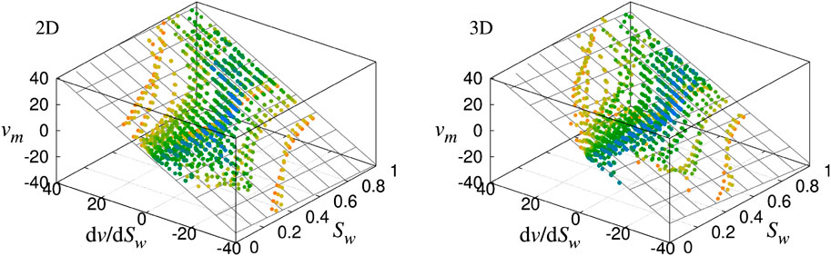
FIGURE 15. Plot of the co-moving velocity $v_m$ as a function of $S_{\text{w}}$ and $\text{d}v/\text{d}{S}_{\text{w}}$ for the square (2D) and Berea (3D) networks. The data shows a rough planner behavior.

6 Summary

We presented a detailed description of a set of algorithms for transporting fluids in a dynamic pore-network model of two-phase flow in porous media. The displacements of the fluids in this model are monitored by updating the positions of all the menisci with time. The fundamental concept of the algorithms is simple, at every time step all the menisci are displaced according to the velocity in the corresponding link and then all the fluids arriving at a node from the incoming links are distributed to the outgoing links. There, the distributed volumes are proportional to the ratio between the velocities in the outgoing links and the ratio between the incoming fluid volumes. We presented these algorithms with all the technical details so that it is possible for the reader to reproduce this model. We have illustrated that this pore-network model and the meniscus algorithms are applicable to both the regular and irregular network topologies in two and three dimensions. By reproducing some of the fundamental results of two-phase flow, we have shown that the model can be used to simulate both the transient and steady-state flow. The model is able to generate different drainage displacement patterns by altering the capillary number and viscosity ratios. In steady state, the model successfully reproduces the linear to non-linear transition in the effective rheological properties as well as the relations between the seepage velocities. For all the results presented here, we used the same meniscus dynamics algorithms without any modification.

Apart from the standard applications of two-phase flow, this model can also be very useful to study the effect of the pore-scale dynamics at low capillary numbers, such as the retractions of menisci after a Haines jump and the long-range capillary effects, which are not possible to capture with the quasi-static or percolation-based models as observed experimentally in [46]. There is also a number of possibilities for further developments. In a recent paper by Zhao et al. [4] ten different groups with different approaches to model two-phase flow in porous media were invited to reproduce fluid injection in a circular Hele-Shaw cell at different capillary numbers and wetting properties, ranging from drainage to strong imbibition, i.e., imbibition where film flow dominates the process. The conclusion of that work was, whereas all the different approaches were able to reproduce the drainage processes well, none succeeded in reproducing strong imbibition. An important mechanism during imbibition is wetting film flow along pore walls. Our presented work accounts the Darcy-like creep flow and modeling the film flow mechanisms within the same framework can also be done as demonstrated in the first attempt in [73]. Another possible development can be replacing the time integration with a Monte Carlo algorithm as proposed by Savani et al. [74] that can further improve the computational efficiency of this model. However, that method needs to be tested at low capillary numbers and was only been implemented for regular lattices. Other important phenomena such as wetting angle hysteresis is straight-forward to implement. Further applications such as the wettability alteration due to changes in the composition of the immiscible fluids can also be investigated with this model as demonstrated in [65, 66].

Data Availability Statement

The raw data supporting the conclusions of this article will be made available by the authors, without undue reservation.

Author Contributions

The meniscus algorithms in their latest form was developed by SS in collaboration with MG, MV, and AH. SS performed all the numerical simulations and the results were analyzed by all the authors. The analytical part related to the relation between the seepage velocities was developed by AH. SS wrote the first draft of the manuscript which then updated to its final form by all the authors.

Funding

SS was supported by the National Natural Science Foundation of China under grant number 11750110430. This work was partly supported by the Research Council of Norway through its Center of Excellence funding scheme, project number 262644.

Conflict of Interest

The authors declare that the research was conducted in the absence of any commercial or financial relationships that could be construed as a potential conflict of interest.

Acknowledgments

We thank our co-workers, past and present, who have been involved in developing this model through its various stages, Eyvind Aker, G. George Batrouni, Morten Grøva, Henning A. Knudsen, Knut Jørgen Måløy, Pål Eric Øren, Thomas Ramstad, Subhadeep Roy, Isha Savani and Glen Tørå.

References

1. Dullien FAL. Porous media: fluid transport and pore structure. San Diego, CA: Academic Press (1992)

Google Scholar

2. Bear J. Dynamics of fluids in porous media. Mineola, NY: Dover (1988).

Google Scholar

3. Løvoll G, Méheust Y, Toussaint R, Schmittbuhl J, Måløy KJ. Growth activity during fingering in a porous Hele-Shaw cell. Phys Rev E - Stat Nonlinear Soft Matter Phys (2004) 70:026301. doi:10.1103/PhysRevE.70.026301

CrossRef Full Text | Google Scholar

4. Zhao B, MacMinn CW, Primkulov BK, Y Chen, Valocchi AJ, Zhao J, et al. Comprehensive comparison of pore-scale models for multiphase flow in porous media. Proc Natl Acad Sci USA (2019) 116:13799. doi:10.1073/pnas.1901619116

PubMed Abstract | CrossRef Full Text | Google Scholar

5. Lenormand R, Touboul E, Zarcone C. Numerical models and experiments on immiscible displacements in porous media. J Fluid Mech (1988) 189:165. doi:10.1017/S0022112088000953

CrossRef Full Text | Google Scholar

6. Måløy KJ, Feder J, Jøssang T. Viscous fingering fractals in porous media. Phys Rev Lett (1985) 55:2688. doi:10.1103/PhysRevLett.55.2688

PubMed Abstract | CrossRef Full Text | Google Scholar

7. Wilkinson D, Willemsen JF. Invasion percolation: a new form of percolation theory. J Phys Math Gen (1983) 16:3365. doi:10.1088/0305-4470/16/14/028

CrossRef Full Text | Google Scholar

8. Lenormand R, Zarcone C. Invasion percolation in an etched network: measurement of a fractal dimension, Phys Rev Lett (1985) 54:2226. doi:10.1103/PhysRevLett.54.2226

PubMed Abstract | CrossRef Full Text | Google Scholar

9. Witten TA, Sander LM. Diffusion-limited aggregation, a kinetic critical phenomenon. Phys Rev E (1981) 47:1400. doi:10.1103/PhysRevLett.47.1400

CrossRef Full Text | Google Scholar

10. Paterson L. Diffusion-limited aggregation and two-fluid displacements in porous media. Phys Rev Lett (1984) 52:1621. doi:10.1103/PhysRevLett.52.1621

CrossRef Full Text | Google Scholar

11. Tallakstad KT, Knudsen HA, Ramstad T, Løvoll G, Måløy KJ, Toussaint R, Flekkøy EG, et al. Steady-state two-phase flow in porous media: statistics and transport properties. Phys Rev Lett (2009) 102:074502. doi:10.1103/PhysRevLett.102.074502

PubMed Abstract | CrossRef Full Text | Google Scholar

12. Tallakstad KT, Løvoll G, Knudsen HA, Ramstad T, Flekkøy EG, Måløy KJ. Steady-state, simultaneous two-phase flow in porous media: an experimental study. Phys Rev E - Stat Nonlinear Soft Matter Phys (2009) 80:036308. doi:10.1103/PhysRevE.80.036308

CrossRef Full Text | Google Scholar

13. Rassi EM, Codd SL, Seymour JD. Nuclear magnetic resonance characterization of the stationary dynamics of partially saturated media during steady-state infiltration flow. New J Phys (2011) 13:015007. doi:10.1088/1367-2630/13/1/015007

CrossRef Full Text | Google Scholar

14. Sinha S, Hansen A. Effective rheology of immiscible two-phase flow in porous media. Europhys Lett (2012) 99:44004. doi:10.1209/0295-5075/99/44004

CrossRef Full Text | Google Scholar

15. Sinha S, Bender AT, Danczyk M, Keepseagle K, Prather CA, Bray JM, et al. Effective rheology of two-phase flow in three-dimensional porous media: experiment and simulation. Transport Porous Media (2017) 119:77. doi:10.1007/s11242-017-0874-4

PubMed Abstract | CrossRef Full Text | Google Scholar

16. Gao Y, Lin Q, Bijeljic B, Blunt MJ. Pore-scale dynamics and the multiphase Darcy law. Phys Rev Fluids (2020) 5:013801. doi:10.1103/physrevfluids.5.013801

CrossRef Full Text | Google Scholar

17. Chen JD, Wilkinson D. Pore-scale viscous fingering in porous media, Phys Rev Lett (1985) 55:1892. doi:10.1103/PhysRevLett.55.1892

PubMed Abstract | CrossRef Full Text | Google Scholar

18. Saffman PG, Taylor GI. The penetration of a fluid into a porous medium or Hele-Shaw cell containing a more viscous liquid. Proc. Royal Soc. A: Math. Phys. Eng. Sc. (1958) 245:312. doi:10.1098/rspa.1958.0085

CrossRef Full Text | Google Scholar

19. Bensimon D, Kadanoff LP, Liang S, Shraiman BI, Tang C. Viscous flows in two dimensions. Rev Mod Phys (1986) 58:977. doi:10.1103/RevModPhys.58.977

CrossRef Full Text | Google Scholar

20. Koplik J, Lasseter TJ. Two-phase flow in random network models of porous media. Soc Petrol Eng J (1985) 25:89. doi:10.2118/11014-PA

CrossRef Full Text | Google Scholar

21. Gjennestad MA, Winkler M, Hansen A. Pore network modeling of the effects of viscosity ratio and pressure gradient on steady-state incompressible two-phase flow in porous media. Transp. Porous Med (2020) 132 (2):355–379. doi:10.1007/s11242-020-01395-z

CrossRef Full Text | Google Scholar

22. Hassanizadeh SM, Gray WG. Toward an improved description of the physics of two-phase flow. Adv Water Resour (1993) 16:53. doi:10.1016/0309-1708(93)90029-F

CrossRef Full Text | Google Scholar

23. Hilfer R. Macroscopic equations of motion for two-phase flow in porous media. Phys Rev E (1998) 58:2090. doi:10.1103/PhysRevE.58.2090

CrossRef Full Text | Google Scholar

24. Gray WG, Miller CT. Introduction to the thermodynamically constrained averaging theory for porous medium systems. Berlin, Germany: Springer (2014)

Google Scholar

25. Hansen A, Sinha S, Bedeaux D, Kjelstrup S, Gjennestad MA, Vassvik M. Relations between seepage velocities in immiscible, incompressible two-phase flow in porous media. Transport Porous Media (2018) 125:565. doi:10.1007/s11242-018-1139-6

CrossRef Full Text | Google Scholar

26. Raeini AQ, Blunt MJ, Bijeljic B. Modelling two-phase flow in porous media at the pore scale using the volume-of-fluid method. J Comput Phys (2012) 231:5653. doi:10.1016/j.jcp.2012.04.011

CrossRef Full Text | Google Scholar

27. Jettestuen E, Helland JO, Prodanovic M. A level set method for simulating capillary-controlled displacements at the pore scale with nonzero contact angles. Water Resour Res (2013) 49:4645. doi:10.1002/wrcr.20334

CrossRef Full Text | Google Scholar

28. Gjennestad MA, Munkejord ST. Modelling of heat transport in two-phase flow and of mass transfer between phases using the level-set method. Energy Proc (2015) 64:53. doi:10.1016/j.egypro.2015.01.008

CrossRef Full Text | Google Scholar

29. Gunstensen AK, Rothman DH, Zaleski S, Zanetti G. Lattice Boltzmann model of immiscible fluids. Phys Rev A (1991) 43:4320. doi:10.1103/PhysRevA.43.4320

PubMed Abstract | CrossRef Full Text | Google Scholar

30. Ramstad T, Øren PE, Bakke S. Simulation of two-phase flow in reservoir rocks using a lattice Boltzmann method. SPE J (2010) 15:917. doi:10.2118/124617-PA

CrossRef Full Text | Google Scholar

31. Aursjø O, Løvoll G, Knudsen HA, Flekkøy EG, Måløy KJ. A direct comparison between a slow pore scale drainage experiment and a 2D lattice Boltzmann simulation. Transport Porous Media (2011) 86:125. doi:10.1007/s11242-010-9611-y

CrossRef Full Text | Google Scholar

32. Blunt MJ. Flow in porous media-pore-network models and multiphase flow. Curr Opin Colloid Interface Sci (2001) 6:197. doi:10.1016/S1359-0294(01)00084-X

CrossRef Full Text | Google Scholar

33. Joekar-Niasar V, Hassanizadeh SM. Analysis of fundamentals of two-phase flow in porous media using dynamic pore-network models: a review. Crit Rev Environ Sci Technol (2012) 42:1895. doi:10.1080/10643389.2011.574101

CrossRef Full Text | Google Scholar

34. Chandler R, Koplik J, Lerman K, Willemsen JF. Capillary displacement and percolation in porous media. J Fluid Mech (1982) 119:249. doi:10.1017/S0022112082001335

CrossRef Full Text | Google Scholar

35. Blunt MJ. Physically-based network modeling of multiphase flow in intermediate-wet porous media. J Petrol Sci Eng (1999) 20:117. doi:10.1016/S0920-4105(98)00010-2

CrossRef Full Text | Google Scholar

36. Cieplak M, Robbins MO. Dynamical transition in quasistatic fluid invasion in porous media. Phys Rev Lett (1988) 60:2042. doi:10.1103/PhysRevLett.60.2042

PubMed Abstract | CrossRef Full Text | Google Scholar

37. Cieplak M, Robbins MO. Influence of contact angle on quasistatic fluid invasion of porous media. Phys Rev B Condens Matter (1990) 41:11508. doi:10.1103/PhysRevB.41.11508

PubMed Abstract | CrossRef Full Text | Google Scholar

38. Øren P-E, Bakke S, Arntzen OJ. Extending predictive capabilities to network models. SPE J (1998) 3:324. doi:10.2118/52052-PA

CrossRef Full Text | Google Scholar

39. Blunt MJ, Jackson MD, Piri M, Valvatne PH. Detailed physics, predictive capabilities and macroscopic consequences for pore-network models of multiphase flow. Adv Water Resour (2002) 25:1069. doi:10.1016/S0309-1708(02)00049-0

CrossRef Full Text | Google Scholar

40. Primkulov BK, Talman S, Khaleghi K, Shokri AR, Chalaturnyk R, Zhao B, et al. Quasistatic fluid-fluid displacement in porous media: invasion-percolation through a wetting transition. Phys. Rev. Fluids (2018) 3:104001. doi:10.1103/PhysRevFluids.3.104001

CrossRef Full Text | Google Scholar

41. Joekar-Niasar V, Hassanizadeh SM, Dahle H. Non-equilibrium effects in capillarity and interfacial area in two-phase flow: dynamic pore-network modelling. J Fluid Mech (2010) 655:38. doi:10.1017/S0022112010000704

CrossRef Full Text | Google Scholar

42. Hammond PS, Unsal E. A dynamic pore network model for oil displacement by wettability-altering surfactant solution. Transport Porous Media (2012) 92:789. doi:10.1007/s11242-011-9933-4

CrossRef Full Text | Google Scholar

43. Aker E, Måløy KJ, Hansen A, Batrouni GG. A two-dimensional network simulator for two-phase flow in porous media. Transport Porous Media (1998) 32:163. doi:10.1023/A:1006510106194

CrossRef Full Text | Google Scholar

44. Haines WB. Studies in the physical properties of soil. v. the hysteresis effect in capillary properties, and the modes of moisture distribution associated therewith. J Agric Sci (1930) 20:97. doi:10.1017/S002185960008864X

CrossRef Full Text | Google Scholar

45. Berg S, Ott H, Klapp SA, Schwing A, Neiteler R, Brussee N Real-time 3D imaging of Haines jumps in porous media flow. Proc Natl Acad Sci USA (2013) 110:3755. doi:10.1073/pnas.1221373110

PubMed Abstract | CrossRef Full Text | Google Scholar

46. Armstrong RT, Berg S. Interfacial velocities and capillary pressure gradients during haines jumps. Phys Rev E - Stat Nonlinear Soft Matter Phys (2013) 88:043010. doi:10.1103/PhysRevE.88.043010

CrossRef Full Text | Google Scholar

47. Måløy KJ, Furuberg L, Feder J, Jøssang T. Dynamics of slow drainage in porous media. Phys Rev Lett (1992) 68:2161. doi:10.1103/PhysRevLett.68.2161

CrossRef Full Text | Google Scholar

48. Knudsen HA, Aker E, Hansen A. Bulk flow regimes and fractional flow in 2D porous media by numerical simulations. Trannsp. Porous Med (2002) 47:99. doi:10.1023/A:1015039503551

CrossRef Full Text | Google Scholar

49. Ramstad T, Hansen A, Øren PE. Flux-dependent percolation transition in immiscible two-phase flows in porous media. Phys Rev E - Stat Nonlinear Soft Matter Phys (2009) 79:036310. doi:10.1103/PhysRevE.79.036310

CrossRef Full Text | Google Scholar

50. Erpelding M, Sinha S, Tallakstad KT, Hansen A, Flekkøy EG, Måløy KJ. History independence of steady state in simultaneous two-phase flow through two-dimensional porous media. Phys Rev E - Stat Nonlinear Soft Matter Phys (2013) 88:053004. doi:10.1103/PhysRevE.88.053004

CrossRef Full Text | Google Scholar

51.https://www.imperial.ac.uk/earth-science/research/research-groups/perm/research/pore-scale-modelling/micro-ct-images-and-networks/

Google Scholar

52. Vogel HJ, Roth K. Quantitative morphology and network representation of soil pore structure. Adv Water Resour (2001) 24:233. doi:10.1016/S0309-1708(00)00055-5

CrossRef Full Text | Google Scholar

53. Okabe H, Blunt MJ. Pore space reconstruction using multiple-point statistics. J Petrol Sci Eng (2005) 46:121. doi:10.1016/j.petrol.2004.08.002

CrossRef Full Text | Google Scholar

54. Øren P-E, Bakke S. Process based reconstruction of sandstones and prediction of transport properties. Transport Porous Media (2002) 46:311. doi:10.1023/A:1015031122338

CrossRef Full Text | Google Scholar

55. Øren P-E, Bakke S. Reconstruction of berea sandstone and pore-scale modeling of wettability effects. J Petrol Sci Eng (2003) 39:177. doi:10.1016/S0920-4105(03)00062-7

CrossRef Full Text | Google Scholar

56. Dong H. Micro-CT imaging and pore network extraction. [PhD thesis]. London (UK): Imperial College (2007).

Google Scholar

57. Dong H, Blunt MJ. Pore-network extraction from micro-computerized-tomography images. Phys Rev E - Stat Nonlinear Soft Matter Phys (2009) 80:036307. doi:10.1103/PhysRevE.80.036307

CrossRef Full Text | Google Scholar

58. Sinha S, Hansen A, Bedeaux D, Kjelstrup S. Effective rheology of bubbles moving in a capillary tube. Phys Rev E - Stat Nonlinear Soft Matter Phys (2013) 87:025001. doi:10.1103/PhysRevE.87.025001

CrossRef Full Text | Google Scholar

59. Washburn EW. The dynamics of capillary flow. Phys Rev (1921) 17:273. doi:10.1103/PhysRev.17.273

PubMed Abstract | CrossRef Full Text | Google Scholar

60. Mason G, Morrow NR. Capillary behavior of a perfectly wetting liquid in irregular triangular tubes. J Colloid Interface Sci (1991) 141:262. doi:10.1016/0021-9797(91)90321-X

CrossRef Full Text | Google Scholar

61. Langglois WE. Slow viscous flow. New York, NY: The Macmillan Company (1964)

Google Scholar

62. Jia P, Dong M, Dai L, Yao J. Slow viscous flow through arbitrary triangular tubes and its application in modelling porous media flows. Transport Porous Media (2008) 74:153. doi:10.1007/s11242-007-9187-3

CrossRef Full Text | Google Scholar

63. Batrouni GG, Hansen A. Fourier acceleration of iterative processes in disordered systems. J Stat Phys (1988) 52:747. doi:10.1007/BF01019728

CrossRef Full Text | Google Scholar

64. Press WH, Teukolsky SA, Vetterling WT, Flannery BP. Numerical recipes in C: The art of scientific computing. 2nd ed. New York, NY: Cambridge University Press (1992)

Google Scholar

65. Sinha S, Grøva M, Ødegården TB, Skjetne E, Hansen A. Local wettability reversal during steady-state two-phase flow in porous media. Phys Rev E - Stat Nonlinear Soft Matter Phys (2011) 84:037303. doi:10.1103/PhysRevE.84.037303

CrossRef Full Text | Google Scholar

66. Flovik V, Sinha S, Hansen A. Dynamic wettability alteration in immiscible two-phase flow in porous media: effect on transport properties and critical slowing down. Front Phys (2015) 3:86. doi:10.3389/fphy.2015.00086

CrossRef Full Text | Google Scholar

67. Garstecki P, Fuerstman MJ, Stone HA, Whitesides GM. Formation of droplets and bubbles in a microfluidic T-junction-scaling and mechanism of break-up. Lab Chip 6, 437 (2006) doi:10.1039/b510841a

PubMed Abstract | CrossRef Full Text | Google Scholar

68. Gjennestad MA, Vassvik M, Kjelstrup S, Hansen A. Stable and efficient time integration of a dynamic pore network model for two-phase flow in porous media. Front Phys (2018) 6:56. doi:10.3389/fphy.2018.00056

CrossRef Full Text | Google Scholar

69. Sinha S, Gjennestad MA, Vassvik M, Winkler M, Hansen A, Flekkøy EG. Rheology of high-capillary number two-phase flow in porous media. Front Phys (2019) 7:65. doi:10.3389/fphy.2019.00065

CrossRef Full Text | Google Scholar

70. Craig FF The reservoir engineering aspects of waterflooding. Richardson, TX: Monograph Series, Society of Petroleum Engineers (1971)

Google Scholar

71. Dake LP. Fundamentals of reservoir engineering. Amsterdam, Netherlands: Elsevier (1998)

Google Scholar

72. Roy S, Hansen A, Sinha S. Effective rheology of two-phase flow in a capillary fiber bundle model. Front Phys (2019) 7:92. doi:10.3389/fphy.2019.00092

CrossRef Full Text | Google Scholar

73. Tørå G, Øren PE, Hansen A. A dynamic network model for two-phase flow in porous media. Transport Porous Media (2012) 92:145. doi:10.1007/s11242-011-9895-6

CrossRef Full Text | Google Scholar

74. Savani I, Sinha S, Hansen A, Bedeaux D, Kjelstrup S, Vassvik M. A Monte Carlo algorithm for immiscible two-phase flow in porous media. Transport Porous Media (2016) 116:869. doi:10.1007/s11242-016-0804-x

CrossRef Full Text | Google Scholar