Fractional-Order Investigation of Diffusion Equations via Analytical Approach

1 Introduction

Fractional calculus (FC) can be considered as one of the extensions of traditional ordinary calculus. The roots of FC dates back to about 300 years. The idea of fractional calculus arises from the fact that Leibniz used a notation for the nth derivative in his publication as $\left({\text{d}}^{n}y/\text{d}{x}^n\right)$. $L^{\prime }H\widehat{o}pital$ posed a question to Leibniz about the derivative of order $\left(1/2\right)$ in 1,695 [1]. In nature derivatives that involve an integer order are local, whereas a fractional order is nonlocal. The mathematical groundwork for derivatives of a fractional order was laid through the combined efforts of several mathematicians such as Caputo, Miller and Ross, Liouville, Riemann, Podlubny, and others. Later on, several mathematicians devoted their work to this area. Fractional calculus has attracted a lot of interest due to its potential implementations in different scientific areas such as biology, viscoelasticity, engineering, fluid mechanics, and other fields of science [2–10].

From the above applications, mathematicians implemented different methods to solve some vital differential equations of fractional-orders (FDEs), particularly partial differential equations of fractional-orders (FPDEs). FPDEs are considered to be basic mathematical techniques used to model various physical phenomena more precisely than integer-order. The non-linear FPDEs determine different phenomena in engineering and applied sciences. In particular, non-linear FPDEs are the best sources to be utilize in different fields such as material sciences, physics, thermodynamics, chemistry, chemical kinetics, and several other basic processes [11–21]. Various methods to solve FDEs are used in the literature, such as the variational iteration method [22], the modified Adomian decomposition method (MADM) [23], the differential transformation method (DTM) [24], the optimal homotopy asymptotic method (OHAM) [25], and the homotopy perturbation method (HPM) [26].

In 2006, Daftardar-Gejji et al. introduced the iterative method (IM) to solve functional equations [27, 28]. IM is used to solve DEs, of both integers as well fractional-order. In this article, we used the Shehu transform method and the iterative technique and introduced a new technique called the Iterative Shehu Transform method [ISTM] to find the approximate solution of FPDEs. It has been observed that the suggested technique has a simple and effective implementation compared to other existing methods such as the homotopy perturbation method, the variational iteration method, and the Laplace Adomian decomposition method [29].

The diffusion equation is a PDE which expresses the phenomenon which transforms atoms or molecules from a higher construction. The Fick’s law of diffusion was first described by the physiologist Adolf Fick. Later on, Fick’s law was converted into the Diffusion equation. Researchers generalized the classical Diffusion law to obtain modified Diffusion equations such as the hybrid classical wave equation and slow diffusion [30]. There are several diffusion equation implementations such as filtration, electromagnetism, geochemistry, phase transition, cosmology, biochemistry, acoustics, and dynamics of biological groups [31].

In the present paper, we apply ISTM to solve diffusion equations of the form.

(1) One-dimensional diffusion equation having fractional-order of the form:

$\frac{{\partial }^{\alpha }\mu }{\partial {\tau }^{\alpha }}=\frac{{\partial }^2\mu }{\partial {\vartheta }^2}-\frac{\partial \mu }{\partial \vartheta }+\mu \frac{{\partial }^2\mu }{\partial {\vartheta }^2}-{\mu }^2+\mu ,0<\alpha \le 1,\tau \ge 0.$

Have the initial values

$\mu \left(\vartheta ,0\right)=g\left(\vartheta \right).$

(2) Two-dimensional diffusion equation with a fractional-order of the form:

$\frac{{\partial }^{\alpha }\mu }{\partial {\tau }^{\alpha }}=\frac{{\partial }^2\mu }{\partial {\vartheta }^2}+\frac{{\partial }^2\mu }{\partial {\zeta }^2},0<\alpha \le 1,\tau \ge 0.$

Have the initial values

$\mu \left(\vartheta ,\zeta ,0\right)=g\left(\vartheta ,\zeta \right).$

(3) Three-dimensional diffusion equation with a fractional-order of the form:

$\frac{{\partial }^{\alpha }\mu }{\partial {\tau }^{\alpha }}=\frac{{\partial }^2\mu }{\partial {\vartheta }^2}+\frac{{\partial }^2\mu }{\partial {\zeta }^2}+\frac{{\partial }^2\mu }{\partial {\omega }^2},0<\alpha \le 1,\tau \ge 0.$

Have the initial values

$\mu \left(\vartheta ,\zeta ,\omega ,0\right)=g\left(\vartheta ,\zeta ,\omega \right).$

2 Preliminaries

In this section, important definitions regarding the present research article are presented.

2.1 Definition

Fractional derivative Caputo operator is given as [7, 8].

$D_{\phi }^{\alpha }\mu \left(\vartheta ,\phi \right)=\frac{1}{\Gamma \left(k-\alpha \right)}{\displaystyle {\int }_0^{\phi }{\left(\phi -\rho \right)}^{k-\alpha -1}{\mu }^{\left(k\right)}\left(\vartheta ,\rho \right)\text{d}\rho },k-1<\alpha \le k,k\in N.$

2.2 Definition

Riemann-Liouville fractional integral [7, 8].

$I_{\tau }^{\alpha }g\left(\vartheta ,\tau \right)=\frac{1}{\Gamma \left(\alpha \right)}{\displaystyle {\int }_0^{\tau }{\left(\tau -\rho \right)}^{\alpha -1}g\left(\vartheta ,\rho \right)\text{d}\rho ,}\rho >0\left(k-1<\alpha \le k\right),k\in N.$

$I_{\tau }^{\alpha }$ stands for fractional integral.

2.3 Definition

Shehu transform (ST) [32–35].

Shehu transform function in set A is expressed by

$A=\{\nu \left(\tau \right):\exists ,{\rho }_1,{\rho }_2>0,\left|\nu \left(\tau \right)\right|\Vert <M{e}^{\left(\left|\tau \right|/{\rho }_i\right)},,\text{if} \tau \in \left[0,\infty \right).(1)$

The Shehu transformation which is defined by $S(.)$ for a function $\nu \left(\tau \right)$ is expressed as [32–35].

$S\left\{\nu \left(\tau \right)\right\}=V\left(s,\mu \right)={\displaystyle {\int }_0^{\infty }\nu \left(\tau \right)e^{\left(-s\tau /\mu \right)}\left(\tau \right)\text{d}\tau },\tau >0 s>0.(2)$

The Shehu transformation of a function $\nu \left(\tau \right)$ is $V\left(s,\mu \right)$: then $\nu \left(\tau \right)$ is called the inverse of $V\left(s,\mu \right)$ which is defined as

$S^{-1}\left\{V\left(s,\mu \right)\right\}=\nu \left(\tau \right),\text{for} \tau \ge 0, S^{-1}\text{is} \text{inverse} \text{Shehu}\text{ transformation}.(3)$

2.4 Definition

The fractional derivative in terms of ST [32–35].

The ST of the fractional derivative is described as

$S\left\{{\nu }^{\left(\alpha \right)}\left(\tau \right)\right\}=\frac{s^{\alpha }}{u^{\alpha }}V\left(s,u\right)-{\displaystyle \sum _{k=0}^{n-1}\left(\frac{s}{u}\right){\nu }^{\left(k\right)}{\left(0\right)}^{\alpha -k-1}},0<\alpha \le n.(4)$

2.5 Definition

The Mittag-Leffler function is expressed as [7, 8].

$E_{\alpha }\left(\omega \right)={\displaystyle \sum }_{q=0}^{\infty }\frac{{\omega }^q}{\Gamma \left(\alpha q+1\right)},\left(\alpha \in C,\mathrm{Re}\left(\alpha \right)>0\right).$

A further generalization of the equation is given in the form of

$E_{\alpha ,\beta }\left(\omega \right)={\displaystyle \sum _{q=0}^{\infty }\frac{{\omega }^q}{\Gamma \left(\alpha q+\beta \right)}};\left(\alpha ,\beta \in C,\mathrm{Re}\left(\alpha \right)>0\right),\mathrm{Re}\left(\beta \right)>0).$

3 Idea of ISTM

In this section, we use ISTM to determine the general solution of fractional-order diffusion equations [32–35].

$D_{\tau }^{\alpha }\mu \left(\vartheta ,\zeta ,\tau \right)+R\mu \left(\vartheta ,\zeta ,\tau \right)+N\mu \left(\vartheta ,\zeta ,\tau \right)=g\left(\vartheta ,\zeta ,\tau \right),k-1<\alpha \le k,k\in N,(5)$

${\mu }^i\left(\vartheta ,\zeta ,o\right)=h_i\left(\vartheta ,\zeta \right),i=\mathrm{0,1,2},\dots ,m-1,(6)$

where $D_{\tau }^{\alpha }\mu \left(\vartheta ,\zeta ,\tau \right)$ is the fractional-order Caputo derivative, $k-1<\alpha \le k$, explained by Eq. 5, R is a linear and N a non-linear operator while $p\left(\vartheta ,\zeta ,\tau \right)$ is an analytic function.

Applying Shehu transformation to Eq. 5, we obtain [32–35].

$S\left[D_{\tau }^{\alpha }\mu \left(\vartheta ,\zeta ,\tau \right)\right]+S\left[R\mu \left(\vartheta ,\zeta ,\tau \right)+N\mu \left(\vartheta ,\zeta ,\tau \right)\right]=S\left[g\left(\vartheta ,\zeta ,\tau \right)\right],$

and by using the property of Shehu transform differentiation, we obtain

$S\left[\mu \left(\vartheta ,\zeta ,\tau \right)\right]=\frac{u^{\alpha }}{s^{\alpha }}{\displaystyle \sum _{k=0}^{m-1}{\left(\frac{s}{u}\right)}^{\alpha -1-k}{\mu }^k\left(\vartheta ,\zeta ,0\right)+\frac{u^{\alpha }}{s^{\alpha }}S\left[g\left(\vartheta ,\zeta ,\tau \right)\right]-\frac{u^{\alpha }}{s^{\alpha }}S\left[R\mu \left(\vartheta ,\zeta ,\tau \right)+N\mu \left(\vartheta ,\zeta ,\tau \right)\right]}.(7)$

On taking inverse Shehu transform of Eq. 7, we obtain [32–35].

$\mu \left(\vartheta ,\zeta ,\tau \right)=S^{-1}\left[\frac{u^{\alpha }}{s^{\alpha }}\left({\displaystyle \sum _{k=0}^{m-1}{s}^{\alpha -1-k}{\mu }^k\left(\vartheta ,\zeta ,0\right)+S\left[g\left(\vartheta ,\zeta ,\tau \right)\right]}\right)\right]-S^{-1}\left[\frac{u^{\alpha }}{s^{\alpha }}S\left[R\mu \left(\vartheta ,\zeta ,\tau \right)+N\mu \left(\vartheta ,\zeta ,\tau \right)\right]\right].(8)$

Now, applying the iterative method,

$\mu \left(\vartheta ,\zeta ,\tau \right)={\displaystyle \sum _{i=0}^{\infty }{\mu }_i\left(\vartheta ,\zeta ,\tau \right)}.(9)$

In Eq. 9, the linear and nonlinear parts R and N, respectively, are decomposed as follows Eqs. 11, 12

$R\left({\displaystyle \sum _{i=0}^{\infty }{\mu }_i\left(\vartheta ,\zeta ,\tau \right)}\right)={\displaystyle \sum _{i=0}^{\infty }R\left[{\mu }_i\left(\vartheta ,\zeta ,\tau \right)\right]},(10)$

$N\left({\displaystyle \sum _{i=0}^{\infty }{\mu }_i\left(\vartheta ,\zeta ,\tau \right)}\right)=N\left[{\mu }_0\left(\vartheta ,\zeta ,\tau \right)\right]+{\displaystyle \sum _{i=1}^{\infty }\left\{N\left({\displaystyle \sum _{k=0}^i{\mu }_k(\vartheta ,\zeta ,\tau }\right)-N\left({\displaystyle \sum _{k=0}^{i-1}{\mu }_k\left(\vartheta ,\zeta ,\tau \right)}\right)\right\}}.(11)$

Substituting Eqs. 9, 11 in Eq. 8 yields

${\displaystyle \sum }_{i=0}^{\infty }{\mu }_i\left(\vartheta ,\zeta ,\tau \right)=S^{-1}\left[\frac{u^{\alpha }}{s^{\alpha }}\left({\displaystyle \sum _{k=0}^{m-1}{\left(\frac{u}{s}\right)}^{\alpha -1-k}{\mu }^k\left(\vartheta ,\zeta ,0\right)+S\left[g\left(\vartheta ,\zeta ,\tau \right)\right]}\right)\right]-S^{-1}\left[\frac{u^{\alpha }}{s^{\alpha }}S\left[{\displaystyle \sum _{i=0}^{\infty }R\left[{\mu }_i\left(\vartheta ,\zeta ,\tau \right)\right]+N\left[{\mu }_0\left(\vartheta ,\zeta ,\tau \right)\right]}+{\displaystyle \sum _{i=1}^{\infty }\left\{N\left({\displaystyle \sum _{k=0}^i{\mu }_k\left(\vartheta ,\zeta ,\tau \right)}\right)-N\left({\displaystyle \sum _{k=0}^{i-1}{\mu }_k\left(\vartheta ,\zeta ,\tau \right)}\right)\right\}}\right]\right].(12)$

We set

${\mu }_0\left(\vartheta ,\zeta ,\tau \right)=S^{-1}\left[\frac{u^{\alpha }}{s^{\alpha }}\left({\displaystyle \sum _{k=0}^{m-1}{\left(\frac{u}{s}\right)}^{\alpha -1-k}{\mu }^k\left(\vartheta ,\zeta ,0\right)+\frac{u^{\alpha }}{s^{\alpha }}L\left(g\left(\vartheta ,\zeta ,\tau \right)\right)}\right)\right],(13)$

${\mu }_1\left(\vartheta ,\zeta ,\tau \right)=-S^{-1}\left[\frac{u^{\alpha }}{s^{\alpha }}S\left[R[{\mu }_0\left(\vartheta ,\zeta ,\tau \right)\right]+N\left[{\mu }_0\left(\vartheta ,\zeta ,\tau \right)\right]\right],(14)$

${\mu }_{m+1}\left(\vartheta ,\zeta ,\tau \right)=-S^{-1}\left[\frac{u^{\alpha }}{s^{\alpha }}S\left[R\left({\mu }_m\left(\vartheta ,\zeta ,\tau \right)\right)\left\{N\left({\displaystyle \sum _{k=0}^m{\mu }_k\left(\vartheta ,\zeta ,\tau \right)}\right)-N\left({\displaystyle \sum _{k=0}^{m-1}{\mu }_k\left(\vartheta ,\zeta ,\tau \right)}\right)\right\}\right]\right],m\ge 1.(15)$

However, the m-term approximate solution of Eqs. 5, 6 is determined by

$\mu \left(\vartheta ,\zeta ,\tau \right)\cong {\mu }_0\left(\vartheta ,\zeta ,\tau \right)+{\mu }_1\left(\vartheta ,\zeta ,\tau \right)+{\mu }_2\left(\vartheta ,\zeta ,\tau \right)+\cdots +{\mu }_m\left(\vartheta ,\zeta ,\tau \right),m=\mathrm{1,2},\dots (16)$

4 Applications

In this section, we apply ISTM to obtain the solution of fractional order diffusion equation to show the accuracy and appropriateness of ISTM to solve exactly nonlinear FPDEs.

4.1 Example

Consider diffusion equation of fractional-order in one-dimension [31].

$\frac{{\partial }^{\alpha }\mu }{\partial {\tau }^{\alpha }}=\frac{{\partial }^2\mu }{\partial {\vartheta }^2}-\frac{\partial \mu }{\partial \vartheta }+\mu \frac{{\partial }^2\mu }{\partial {\vartheta }^2}-{\mu }^2+\mu ,0<\alpha \le 1,\tau >0.(17)$

Have the initial values

$\mu \left(\vartheta ,0\right)=\exp \vartheta .(18)$

Applying Shehu transformation to Eq. 17, we obtain

$S\left[\mu \left(\vartheta ,\tau \right)\right]=\frac{1}{s}\text{exp}\vartheta +\frac{u^{\alpha }}{s^{\alpha }}\left[S\left(\frac{{\partial }^2\mu }{\partial {\vartheta }^2}-\frac{\partial \mu }{\partial \vartheta }+\mu \frac{{\partial }^2\mu }{\partial {\vartheta }^2}-{\mu }^2+\mu \right)\right].(19)$

Taking inverse Shehu transform of Eq. 19

$\mu \left(\vartheta ,\tau \right)=\exp \vartheta +S^{-1}\left[\frac{u^{\alpha }}{s^{\alpha }}\left\{S\left(\frac{{\partial }^2\mu }{\partial {\vartheta }^2}-\frac{\partial \mu }{\partial \vartheta }+\mu \frac{{\partial }^2\mu }{\partial {\vartheta }^2}-{\mu }^2+\mu \right)\right\}\right].(20)$

Using iterative technique

$\begin{array}{l}{\mu }_0\left(\vartheta ,\tau \right)=\exp \vartheta ,\\ {\mu }_1\left(\vartheta ,\tau \right)=S^{-1}\left[\frac{u^{\alpha }}{s^{\alpha }}\left\{S\left(\frac{{\partial }^2{\mu }_0}{\partial {\vartheta }^2}-\frac{\partial {\mu }_0}{\partial \vartheta }+{\mu }_0\frac{{\partial }^2{\mu }_0}{\partial {\vartheta }^2}-{\mu }_0^2+{\mu }_0\right)\right\}\right]\\ =\exp \vartheta \frac{{\tau }^{\alpha }}{\Gamma \left(\alpha +1\right)},\end{array}$

$\begin{array}{l}{\mu }_2\left(\vartheta ,\tau \right)=S^{-1}\left[\frac{u^{\alpha }}{s^{\alpha }}\left\{S\left(\frac{{\partial }^2{\mu }_1}{\partial {\vartheta }^2}-\frac{\partial {\mu }_1}{\partial \vartheta }+{\mu }_1\frac{{\partial }^2{\mu }_1}{\partial {\vartheta }^2}-{\mu }_1^2+{\mu }_1\right)\right\}\right]\\ =\exp \vartheta \frac{{\tau }^{2\alpha }}{\Gamma \left(2\alpha +1\right)},\end{array}$

$\begin{array}{l}{\mu }_3\left(\vartheta ,\tau \right)=S^{-1}\left[\frac{u^{\alpha }}{s^{\alpha }}\left\{S\left(\frac{{\partial }^2{\mu }_2}{\partial {\vartheta }^2}-\frac{\partial {\mu }_2}{\partial \vartheta }+{\mu }_2\frac{{\partial }^2{\mu }_2}{\partial {\vartheta }^2}-{\mu }_2^2+{\mu }_2\right)\right\}\right]\\ =\exp \vartheta \frac{{\tau }^{3\alpha }}{\Gamma \left(3\alpha +1\right)},\end{array}$

$\begin{array}{l}{\mu }_4\left(\vartheta ,\tau \right)=S^{-1}\left[\frac{u^{\alpha }}{s^{\alpha }}\left\{S\left(\frac{{\partial }^2{\mu }_3}{\partial {\vartheta }^2}-\frac{\partial {\mu }_3}{\partial \vartheta }+{\mu }_3\frac{{\partial }^2{\mu }_3}{\partial {\vartheta }^2}-{\mu }_3^2+{\mu }_3\right)\right\}\right]\\ =\exp \vartheta \frac{{\tau }^{4\alpha }}{\Gamma \left(4\alpha +1\right)}.\end{array}$

Thus, in the form of a series, the analytical solution can be written as

$\begin{array}{l}\mu \left(\vartheta ,\tau \right)={\mu }_0\left(\vartheta ,\tau \right)+{\mu }_1\left(\vartheta ,\tau \right)+{\mu }_2\left(\vartheta ,\tau \right)+{\mu }_3\left(\vartheta ,\tau \right)+{\mu }_3\left(\vartheta ,\tau \right)+\cdots ,\\ =\exp \vartheta +\exp \vartheta \frac{{\tau }^{\alpha }}{\Gamma \left(\alpha +1\right)}+\exp \vartheta \frac{{\tau }^{2\alpha }}{\Gamma \left(2\alpha +1\right)}+\exp \vartheta \\ \frac{{\tau }^{3\alpha }}{\Gamma \left(3\alpha +1\right)}+\exp \vartheta \frac{{\tau }^{4\alpha }}{\Gamma \left(4\alpha +1\right)}+\cdots ,\end{array}$

$\begin{array}{c}\mu \left(\vartheta ,\tau \right)=\exp \vartheta \left(1+\frac{{\tau }^{\alpha }}{\Gamma \left(\alpha +1\right)}+\frac{{\tau }^{2\alpha }}{\Gamma \left(2\alpha +1\right)}+\frac{{\tau }^{3\alpha }}{\Gamma \left(3\alpha +1\right)}+\frac{{\tau }^{4\alpha }}{\Gamma \left(4\alpha +1\right)}+\cdots ,\right),\\ \mu \left(\vartheta ,\tau \right)=\exp \vartheta {\displaystyle \sum _{k=0}^{\infty }\frac{{\left(t^{\alpha }\right)}^k}{\Gamma \left(k\alpha +1\right)}=\exp \vartheta E_{\alpha }\left(t^{\alpha }\right)}.\end{array}$

When $\alpha =1$, the ISTM solution is

$\mu \left(\vartheta ,\tau \right)=\exp \vartheta {\displaystyle \sum _{k=0}^{\infty }\frac{{\left(t\right)}^k}{k!}}.(21)$

The exact solution is:

$\mu \left(\vartheta ,\tau \right)=\text{exp}\left(\vartheta +\tau \right).$

4.2 Example

Consider diffusion equation of fractional-order in two-dimension [31].

$\frac{{\partial }^{\alpha }\mu }{\partial {\tau }^{\alpha }}=\frac{{\partial }^2\mu }{\partial {\vartheta }^2}+\frac{{\partial }^2\mu }{\partial {\zeta }^2},0<\alpha \le 1,\tau \ge 0,(22)$

Having initial values

$\mu \left(\vartheta ,\zeta ,0\right)=\left(1-\zeta \right)\exp \vartheta .(23)$

Applying Shehu transformation to Eq. 22, we obtain

$S\left[\mu \left(\vartheta ,\zeta ,\tau \right)\right]=\frac{1}{s}\left(1-\zeta \right)\text{exp}\vartheta +\frac{u^{\alpha }}{s^{\alpha }}\left[S\left(\frac{{\partial }^2\mu }{\partial {\vartheta }^2}+\frac{{\partial }^2\mu }{\partial {\zeta }^2}\right)\right].(24)$

Taking inverse Shehu transform of Eq. 24

$\mu \left(\vartheta ,\zeta ,\tau \right)=\left(1-\zeta \right)\exp \vartheta +S^{-1}\left[\frac{u^{\alpha }}{s^{\alpha }}\left\{S\left(\frac{{\partial }^2\mu }{\partial {\vartheta }^2}+\frac{{\partial }^2\mu }{\partial {\zeta }^2}\right)\right\}\right].(25)$

Using an iterative technique

$\begin{array}{l}{\mu }_0\left(\vartheta ,\zeta ,\tau \right)=\left(1-\zeta \right)\exp \vartheta ,\\ {\mu }_1\left(\vartheta ,\zeta ,\tau \right)=S^{-1}\left[\frac{u^{\alpha }}{s^{\alpha }}\left\{S\left(\frac{{\partial }^2{\mu }_0}{\partial {\vartheta }^2}+\frac{{\partial }^2{\mu }_0}{\partial {\zeta }^2}\right)\right\}\right]\\ =\left(1-\zeta \right)\exp \vartheta \frac{{\tau }^{\alpha }}{\Gamma \left(\alpha +1\right)},\end{array}$

$\begin{array}{l}{\mu }_2\left(\vartheta ,\zeta ,\tau \right)=S^{-1}\left[\frac{u^{\alpha }}{s^{\alpha }}\left\{S\left(\frac{{\partial }^2{\mu }_1}{\partial {\vartheta }^2}+\frac{{\partial }^2{\mu }_1}{\partial {\zeta }^2}\right)\right\}\right]\\ =\left(1-\zeta \right)\exp \vartheta \frac{{\tau }^{2\alpha }}{\Gamma \left(2\alpha +1\right)},\end{array}$

$\begin{array}{l}{\mu }_3\left(\vartheta ,\zeta ,\tau \right)=S^{-1}\left[\frac{u^{\alpha }}{s^{\alpha }}\left\{S\left(\frac{{\partial }^2{\mu }_2}{\partial {\vartheta }^2}+\frac{{\partial }^2{\mu }_2}{\partial {\zeta }^2}\right)\right\}\right]\\ =\left(1-\zeta \right)\exp \vartheta \frac{{\tau }^{3\alpha }}{\Gamma \left(3\alpha +1\right)},\end{array}$

$\begin{array}{l}{\mu }_4\left(\vartheta ,\zeta ,\tau \right)=S^{-1}\left[\frac{u^{\alpha }}{s^{\alpha }}\left\{S\left(\frac{{\partial }^2{\mu }_3}{\partial {\vartheta }^2}+\frac{{\partial }^2{\mu }_3}{\partial {\zeta }^2}\right)\right\}\right]\\ =\left(1-\zeta \right)\exp \vartheta \frac{{\tau }^{4\alpha }}{\Gamma \left(4\alpha +1\right)}.\end{array}$

Thus, in the form of a series, the analytical solution can be written as

$\begin{array}{l}\mu \left(\vartheta ,\zeta ,\tau \right)={\mu }_0\left(\vartheta ,\zeta ,\tau \right)+{\mu }_1\left(\vartheta ,\zeta ,\tau \right)+{\mu }_2\left(\vartheta ,\zeta ,\tau \right)+{\mu }_3\left(\vartheta ,\zeta ,\tau \right)+{\mu }_3\left(\vartheta ,\zeta ,\tau \right)+\cdots ,\\ \mu \left(\vartheta ,\zeta ,\tau \right)=\left(1-\zeta \right)\exp \vartheta +\left(1-\zeta \right)\exp \vartheta \frac{{\tau }^{\alpha }}{\Gamma \left(\alpha +1\right)}+\left(1-\zeta \right)\exp \vartheta \frac{{\tau }^{2\alpha }}{\Gamma \left(2\alpha +1\right)}\\ +\left(1-\zeta \right)\exp \vartheta \frac{{\tau }^{3\alpha }}{\Gamma \left(3\alpha +1\right)}+\left(1-\zeta \right)\exp \vartheta \frac{{\tau }^{4\alpha }}{\Gamma \left(4\alpha +1\right)}+\cdots ,\end{array}$

$\begin{array}{c}\mu \left(\vartheta ,\zeta ,\tau \right)=\left(1-\zeta \right)\exp \vartheta \left(1+\frac{{\tau }^{\alpha }}{\Gamma \left(\alpha +1\right)}+\frac{{\tau }^{2\alpha }}{\Gamma \left(2\alpha +1\right)}+\frac{{\tau }^{3\alpha }}{\Gamma \left(3\alpha +1\right)}+\frac{{\tau }^{4\alpha }}{\Gamma \left(4\alpha +1\right)}+\cdots ,\right),\\ \mu \left(\vartheta ,\zeta ,\tau \right)=\left(1-\zeta \right)\exp \vartheta {\displaystyle \sum _{k=0}^{\infty }\frac{{\left(t^{\alpha }\right)}^k}{\Gamma \left(k\alpha +1\right)}}=\left(1-\zeta \right)\exp \vartheta E_{\alpha }\left(t^{\alpha }\right).\end{array}$

When $\alpha =1$, the ISTM solution is

$\mu \left(\vartheta ,\zeta ,\tau \right)=\left(1-\zeta \right)\exp \vartheta {\displaystyle \sum _{k=0}^{\infty }\frac{{\left(t\right)}^k}{k!}}.(26)$

The exact solution in closed form is:

$\mu \left(\vartheta ,\zeta ,\tau \right)=\left(1-\zeta \right)\exp \left(\vartheta +\tau \right).$

4.3 Example

Consider diffusion equation of fractional-order in two-dimension [31].

$\frac{{\partial }^{\alpha }\mu }{\partial {\tau }^{\alpha }}=\frac{{\partial }^2\mu }{\partial {\vartheta }^2}+\frac{{\partial }^2\mu }{\partial {\zeta }^2},0<\alpha \le 1,\tau \ge 0.(27)$

Having initial values

$\mu \left(\vartheta ,\zeta ,0\right)=\exp \left(\vartheta +\zeta \right).(28)$

Applying Shehu transformation to Eq. 27, we obtain

$S\left[\mu \left(\vartheta ,\zeta ,\tau \right)\right]=\frac{1}{s}\exp \left(\vartheta +\zeta \right)+\frac{u^{\alpha }}{s^{\alpha }}\left[S\left(\frac{{\partial }^2\mu }{\partial {\vartheta }^2}+\frac{{\partial }^2\mu }{\partial {\zeta }^2}\right)\right].(29)$

Taking inverse Shehu transform of Eq. 29

$\mu \left(\vartheta ,\zeta ,\tau \right)=\text{exp}\left(\vartheta +\zeta \right)+S^{-1}\left[\frac{u^{\alpha }}{s^{\alpha }}\left\{S\left(\frac{{\partial }^2\mu }{\partial {\vartheta }^2}+\frac{{\partial }^2\mu }{\partial {\zeta }^2}\right)\right\}\right].(30)$

Using iterative technique

$\begin{array}{l}{\mu }_0\left(\vartheta ,\zeta ,\tau \right)=\exp \left(\vartheta +\zeta \right),\\ {\mu }_1\left(\vartheta ,\zeta ,\tau \right)=S^{-1}\left[\frac{u^{\alpha }}{s^{\alpha }}\left\{S\left(\frac{{\partial }^2{\mu }_0}{\partial {\vartheta }^2}+\frac{{\partial }^2{\mu }_0}{\partial {\zeta }^2}\right)\right\}\right]\\ =2\exp \left(\vartheta +\zeta \right)\frac{{\tau }^{\alpha }}{\Gamma \left(\alpha +1\right)},\end{array}$

$\begin{array}{l}{\mu }_2\left(\vartheta ,\zeta ,\tau \right)=S^{-1}\left[\frac{u^{\alpha }}{s^{\alpha }}\left\{S\left(\frac{{\partial }^2{\mu }_1}{\partial {\vartheta }^2}+\frac{{\partial }^2{\mu }_1}{\partial {\zeta }^2}\right)\right\}\right]\\ =4\exp \left(\vartheta +\zeta \right)\frac{{\tau }^{2\alpha }}{\Gamma \left(2\alpha +1\right)},\end{array}$

$\begin{array}{l}{\mu }_3\left(\vartheta ,\zeta ,\tau \right)=S^{-1}\left[\frac{u^{\alpha }}{s^{\alpha }}\left\{S\left(\frac{{\partial }^2{\mu }_2}{\partial {\vartheta }^2}+\frac{{\partial }^2{\mu }_2}{\partial {\zeta }^2}\right)\right\}\right]\\ =8\exp \left(\vartheta +\zeta \right)\frac{{\tau }^{3\alpha }}{\Gamma 3\alpha +1},\end{array}$

${\mu }_4\left(\vartheta ,\zeta ,\tau \right)=S^{-1}\left[\frac{u^{\alpha }}{s^{\alpha }}\left\{S\left(\frac{{\partial }^2{\mu }_3}{\partial {\vartheta }^2}+\frac{{\partial }^2{\mu }_3}{\partial {\zeta }^2}\right)\right\}\right].=16\exp \left(\vartheta +\zeta \right)\frac{{\tau }^{3\alpha }}{\Gamma 4\alpha +1},$

Thus, in the form of a series, the analytical solution can be written as

$\begin{array}{c}\mu \left(\vartheta ,\zeta ,\tau \right)={\mu }_0\left(\vartheta ,\zeta ,\tau \right)+{\mu }_1\left(\vartheta ,\zeta ,\tau \right)+{\mu }_2\left(\vartheta ,\zeta ,\tau \right)+{\mu }_3\left(\vartheta ,\zeta ,\tau \right)+{\mu }_4\left(\vartheta ,\zeta ,\tau \right)+\cdots ,\\ \mu \left(\vartheta ,\zeta ,\tau \right)=\exp \left(\vartheta +\zeta \right)+2\exp \left(\vartheta +\zeta \right)\frac{{\tau }^{\alpha }}{\Gamma \left(\alpha +1\right)}+4\exp \left(\vartheta +\zeta \right)\frac{{\tau }^{2\alpha }}{\Gamma \left(2\alpha +1\right)}+8\exp \left(\vartheta +\zeta \right)\frac{{\tau }^{3\alpha }}{\Gamma \left(3\alpha +1\right)}+16\exp \left(\vartheta +\zeta \right)\frac{{\tau }^{4\alpha }}{\Gamma \left(4\alpha +1\right)}+\cdots ,\end{array}$

$\begin{array}{l}\mu \left(\vartheta ,\zeta ,\tau \right)=\exp \left(\vartheta +\zeta \right)\left(1+\frac{2{\tau }^{\alpha }}{\Gamma \left(\alpha +1\right)}+\frac{{\left(2{\tau }^{\alpha }\right)}^2}{\Gamma \left(2\alpha +1\right)}+\frac{{\left(2{\tau }^{\alpha }\right)}^3}{\Gamma \left(3\alpha +1\right)}+\frac{{\left(2{\tau }^{\alpha }\right)}^4}{\Gamma \left(4\alpha +1\right)}+\cdots ,\right),\\ \mu \left(\vartheta ,\zeta ,\tau \right)=\exp \left(\vartheta +\zeta \right){\displaystyle \sum _{k=0}^{\infty }\frac{{\left(t^{\alpha }\right)}^k}{\Gamma \left(k\alpha +1\right)}=\left(1-\zeta \right)\exp \vartheta E_{\alpha }\left(t^{\alpha }\right)}.\end{array}$

When $\alpha =1$, then the ISTM solution is

$\mu \left(\vartheta ,\zeta ,\tau \right)=\exp \left(\vartheta +\zeta \right){\displaystyle \sum _{k=0}^{\infty }\frac{{\left(t\right)}^k}{k!}}.(31)$

The exact solution is:

$\mu \left(\vartheta ,\zeta ,\tau \right)=\exp \left(\vartheta +\zeta +\tau \right).$

4.4 Example

Consider diffusion equation of fractional-order in three-dimension [31].

$\frac{{\partial }^{\alpha }\mu }{\partial {\tau }^{\alpha }}=\frac{{\partial }^2\mu }{\partial {\vartheta }^2}+\frac{{\partial }^2\mu }{\partial {\zeta }^2}+\frac{{\partial }^2\mu }{\partial {\omega }^2},0<\alpha \le 1,\tau \ge 0.(32)$

Having initial values

$\mu \left(\vartheta ,\zeta ,\omega ,0\right)=\sin \vartheta \sin \zeta \sin \omega .(33)$

Applying Shehu transformation to Eq. 32, we obtain

$S\left[\mu \left(\vartheta ,\zeta ,\omega ,\tau \right)\right]=\frac{1}{s}\sin \vartheta \sin \zeta \sin \omega +\frac{u^{\alpha }}{s^{\alpha }}\left[S\left(\frac{{\partial }^2\mu }{\partial {\vartheta }^2}+\frac{{\partial }^2\mu }{\partial {\zeta }^2}+\frac{{\partial }^2\mu }{\partial {\omega }^2}\right)\right].(34)$

Taking inverse Shehu transform of Eq. 34

$\mu \left(\vartheta ,\zeta ,\omega ,\tau \right)=\sin \vartheta \sin \zeta \sin \omega +S^{-1}\left[\frac{u^{\alpha }}{s^{\alpha }}\left\{S\left(\frac{{\partial }^2\mu }{\partial {\vartheta }^2}+\frac{{\partial }^2\mu }{\partial {\zeta }^2}+\frac{{\partial }^2\mu }{\partial {\omega }^2}\right)\right\}\right].(35)$

Using iterative technique

$\begin{array}{l}{\mu }_0\left(\vartheta ,\zeta ,\omega ,\tau \right)=\sin \vartheta \sin \zeta \sin \omega ,\\ {\mu }_1\left(\vartheta ,\zeta ,\omega ,\tau \right)=S^{-1}\left[\frac{u^{\alpha }}{s^{\alpha }}\left\{S\left(\frac{{\partial }^2{\mu }_0}{\partial {\vartheta }^2}+\frac{{\partial }^2{\mu }_0}{\partial {\zeta }^2}+\frac{{\partial }^2{\mu }_0}{\partial {\omega }^2}\right)\right\}\right]\\ =-3\sin \vartheta \sin \zeta \sin \omega \frac{{\tau }^{\alpha }}{\Gamma \left(\alpha +1\right)},\end{array}$

$\begin{array}{l}{\mu }_2\left(\vartheta ,\zeta ,\omega ,\tau \right)=S^{-1}\left[\frac{u^{\alpha }}{s^{\alpha }}\left\{S\left(\frac{{\partial }^2{\mu }_1}{\partial {\vartheta }^2}+\frac{{\partial }^2{\mu }_1}{\partial {\zeta }^2}+\frac{{\partial }^2{\mu }_1}{\partial {\omega }^2}\right)\right\}\right]\\ ={\left(-3\right)}^2\sin \vartheta \sin \zeta \sin \omega \frac{{\tau }^{2\alpha }}{\Gamma \left(2\alpha +1\right)},\end{array}$

$\begin{array}{l}{\mu }_3\left(\vartheta ,\zeta ,\omega ,\tau \right)=S^{-1}\left[\frac{u^{\alpha }}{s^{\alpha }}\left\{S\left(\frac{{\partial }^2{\mu }_2}{\partial {\vartheta }^2}+\frac{{\partial }^2{\mu }_2}{\partial {\zeta }^2}+\frac{{\partial }^2{\mu }_2}{\partial {\omega }^2}\right)\right\}\right]\\ ={\left(-3\right)}^3\sin \vartheta \sin \zeta \sin \omega \frac{{\tau }^{3\alpha }}{\Gamma \left(3\alpha +1\right)},\\ {\mu }_4\left(\vartheta ,\zeta ,\omega ,\tau \right)=S^{-1}\left[\frac{u^{\alpha }}{s^{\alpha }}\left\{S\left(\frac{{\partial }^2{\mu }_3}{\partial {\vartheta }^2}+\frac{{\partial }^2{\mu }_3}{\partial {\zeta }^2}+\frac{{\partial }^2{\mu }_3}{\partial {\omega }^2}\right)\right\}\right]\\ ={\left(-3\right)}^4\sin \vartheta \sin \zeta \sin \omega \frac{{\tau }^{4\alpha }}{\Gamma \left(4\alpha +1\right)}.\end{array}$

Thus, in the form of a series, the analytical solution can be written as

$\begin{array}{l}\mu \left(\vartheta ,\zeta ,\omega ,\tau \right)={\mu }_0\left(\vartheta ,\zeta ,\omega ,\tau \right)+{\mu }_1\left(\vartheta ,\zeta ,\omega ,\tau \right)+{\mu }_2\left(\vartheta ,\zeta ,\omega ,\tau \right)+{\mu }_3\left(\vartheta ,\zeta ,\omega ,\tau \right)+{\mu }_4\left(\vartheta ,\zeta ,\omega ,\tau \right)+\cdots ,\\ =\text{sin}\vartheta \text{sin}\zeta \text{sin}\omega -3\text{sin}\vartheta \text{sin}\zeta \text{sin}\omega \frac{{\tau }^{\alpha }}{\text{Γ}\left(\alpha +1\right)}+{\left(-3\right)}^2\text{sin}\vartheta \text{sin}\zeta \text{sin}\omega \frac{{\tau }^{2\alpha }}{\text{Γ}\left(2\alpha +1\right)}-{\left(3\right)}^3\text{sin}\vartheta \text{sin}\zeta \text{sin}\omega \frac{{\tau }^{3\alpha }}{\text{Γ}\left(3\alpha +1\right)}+{\left(3\right)}^4\text{sin}\vartheta \text{sin}\zeta \text{sin}\omega \frac{{\tau }^{4\alpha }}{\text{Γ}\left(4\alpha +1\right)}+\cdots ,\end{array}$

$\mu \left(\vartheta ,\zeta ,\omega ,\tau \right)=\sin \vartheta \sin \zeta \sin \omega \left(1-\frac{3{\tau }^{\alpha }}{\Gamma \left(\alpha +1\right)}+\frac{{\left(-3{\tau }^{\alpha }\right)}^2}{\Gamma \left(2\alpha +1\right)}+\frac{{\left(-3{\tau }^{\alpha }\right)}^3}{\Gamma \left(3\alpha +1\right)}+\frac{{\left(-3{\tau }^{\alpha }\right)}^4}{\Gamma \left(4\alpha +1\right)}+\cdots ,\right).$

When $\alpha =1,$ then the ISTM solution in a closed form:

$\mu \left(\vartheta ,\zeta ,\omega ,\tau \right)=\sin \vartheta \sin \zeta \sin \omega \left(1-3\tau +\frac{{\left(-3\tau \right)}^2}{2!}+\frac{{\left(-3\tau \right)}^3}{3!}+\frac{{\left(-3\tau \right)}^4}{4!}+\cdots ,\right).$

The exact solution is:

$\mu \left(\vartheta ,\zeta ,\omega ,\tau \right)={\exp }^{-3\tau }\sin \vartheta \sin \zeta \sin \omega .(36)$

5 Conclusion

In the present article, the fractional view analysis is analyzed using an efficient analytical technique. Fractional derivatives are expressed in a Caputo sense. The present method is tested to solve diffusion equation of fractional-order. After investigation, we show that the present method is the best tool to use to solve nonlinear fractional order problems. The exact and obtained solutions in closed contact has verified the reliability of the present technique. Moreover, the graphical representation has confirmed the convergence of the approximate solutions toward the exact solutions and provide the closed form solutions of the targeted problems. The convergence phenomenon has confirmed the reliability of the suggested method.if

FIGURE 1

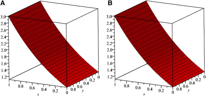
FIGURE 1. Exact solution (A) Exact (B) ISTM solutions of example one at $\alpha =1$. In Figure 1, the Exact and ISTM solutions of Example 1, at α=1 are plotted by using sub-graphs A and B respectively. The graphical representation has shown the closed contact between the exact and ISTM solutions.

FIGURE 2

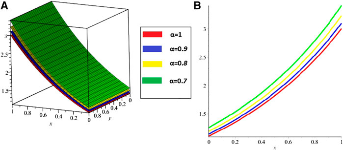
FIGURE 2. ISTM solution of example 1 (C) at various fractional-order α (D) the fractional-order solutions at $\xi =0.5$. In Figure 2, the ISTM solutions at different values of α are presented. The sub-graphs (C) and (D) represents 3D and 2D plots of fractional order solutions of Example 1. The convergence of the fractional solutions towards integer solutions is observed.

FIGURE 3

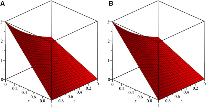
FIGURE 3. Exact solution (A) Exact (B) ISTM solutions of example 2 at $\alpha =1$. In Figure 3, the Exact and ISTM solutions of Example 2, at α=1 are plotted by using sub-graphs A and B respectively. The graphical representation has shown the closed contact between the exact and ISTM solutions of Example 2.

FIGURE 4

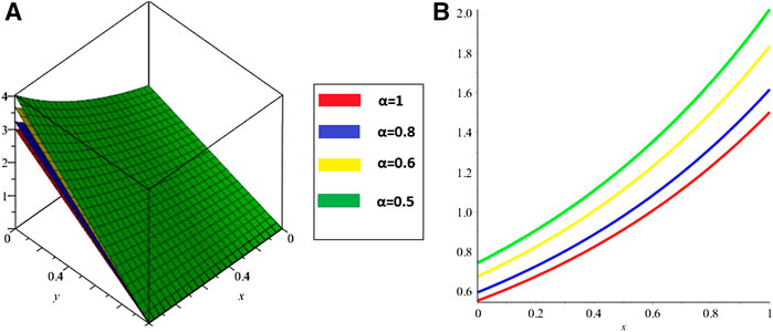
FIGURE 4. ISTM solution of example 2 (C) at various fractional-order α (D) the fractional-order solutions at $\xi =0.5$. In Figure 4, the ISTM solutions of Example 2 at different values of α are presented. The sub-graphs (C) and (D) represents 3D and 2D plots of fractional order solutions of Example 2. The convergence of the fractional solutions towards integer solutions is observed.

FIGURE 5

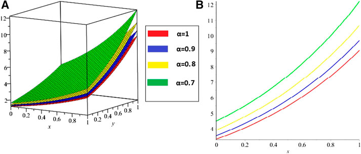
FIGURE 5. ISTM solution of example 3 (A) at various fractional-order α (B) the fractional-order solutions at $\xi =0.5$. In Figure 5, the ISTM solutions of Example 3 at different values of α are presented. The sub-graphs (A) and (B) represents 3D and 2D plots of fractional order solutions of Example 3. The convergence of the fractional solutions towards integer solutions is observed.

FIGURE 6

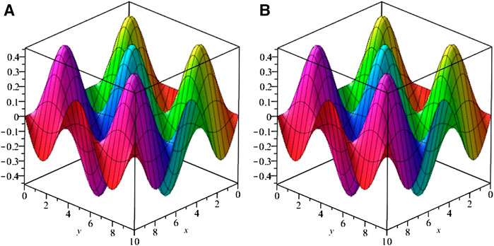
FIGURE 6. Exact solution (A)(B) ISTM solutions of example 4 at $\alpha =1$. In Figure 6, the Exact and ISTM solutions of Example 4, at α=1 are plotted by using sub-graphs A and B respectively. The graphical representation has shown the closed contact between the exact and ISTM solutions of Example 4.

FIGURE 7

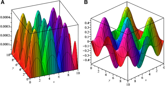
FIGURE 7. (C) Error graph (D) ISTM solutions of example 4 at $\alpha =\mathrm{0,5}$. In Figure 7, the sub-graphs (C) and (D) represent the ISTM Error and solution graphs of Example 4 respectively. The error graph has confirmed the higher accuracy of ISTM.

Data Availability Statement

Publicly available datasets were analyzed in this study. This data can be found here: N/A.

Author Contributions

Conceptualization, HK and SM; Methodology, HL; Software, LM; Validation, DB and HK; Formal Analysis, SM; Investigation, HK; Resources, HK; Writing—Original Draft Preparation, SM; Writing—Review and Editing, HK; Visualization, DB; Supervision, HK, DB; Project Administration, HL; Funding Acquisition, HL and LM

Conflict of Interest

The authors declare that the research was conducted in the absence of any commercial or financial relationships that could be construed as a potential conflict of interest.

Funding

Key Project of Science and Technology Plan of Sichuan Provincial Science and Technology Department (2017JY0199), Project of Education Department of Sichuan Province (JG2018-736).

References

1. Machado JAT, Baleanu D, Chen W, Sabatier J. New trends in fractional dynamics. J Vib Contr (2014) 20:963. doi:10.1177/1077546313507652

CrossRef Full Text | Google Scholar

2. Dumitru B, Kai D, Enrico S, Juan JT. Fractional calculus: models and numerical methods. World Sci (2012) 3:426. doi:10.1142/10044

CrossRef Full Text | Google Scholar

3. Khan H, Khan A, Al-Qurashi M, Shah R, Baleanu D. Modified modelling for heat like equations within Caputo operator. Energies (2020) 13(8):2002. doi:10.3390/en13082002

CrossRef Full Text | Google Scholar

4. Khan H, Shah R, Baleanu D, Kumam P, Arif M. Analytical solution of fractional-order hyperbolic telegraph equation, using natural transform decomposition method. Electronics (2019) 8(9):1015. doi:10.3390/electronics8091015

CrossRef Full Text | Google Scholar

5. Shah R, Khan H, Kumam P, Arif M. An analytical technique to solve the system of nonlinear fractional partial differential equations. Mathematics (2019) 7(6):505. doi:10.3390/math7060505

CrossRef Full Text | Google Scholar

6. Syam MI. Analytical solution of the fractional Fredholm integrodifferential equation using the fractional residual power series method. Complexity (2017) 2017:1–6. doi:10.1155/2017/4573589

CrossRef Full Text | Google Scholar

7. Ye H, Huang R. On the nonlinear fractional differential equations with Caputo sequential fractional derivative. Adv Math Phy (2015) 2015:1–9. doi:10.1155/2015/174156

CrossRef Full Text | Google Scholar

8. Podlubny I. Fractional differential equations: an introduction to fractional derivatives, fractional differential equations, to methods of their solution and some of their applications, Vol 198. Amsterdam, Netherlands: Elsevier (1998)

9. Sabatier JATMJ, Agrawal OP, Machado JT. Advances in fractional calculus, Vol. 4. Dordrecht, Netherlands: Springer (2007).

10. Baleanu D, Diethelm K, Scalas E, Trujillo JJ. Fractional calculus, vol 3 of series on complexityNonlinearity and Chaos. Singapore: World Scientific (2012)

11. Srivastava HM, Shah R, Khan H, Arif M. Some analytical and numerical investigation of a family of fractional‐order Helmholtz equations in two space dimensions. Math Methods Appl Sci (2020) 43(1):199–212. doi:10.1002/mma.5846

CrossRef Full Text | Google Scholar

12. Khan H, Shah R, Arif M, Bushnaq S. The Chebyshev wavelet method (CWM) for the numerical solution of fractional HIV infection of CD4+ T cells model. Int J Algorithm Comput Math (2020) 6(2):1–17. doi:10.1007/s40819-020-0786-9

CrossRef Full Text | Google Scholar

13. Shah R, Khan H, Baleanu D, Kumam P, Arif M. A semi-analytical method to solve family of Kuramoto-Sivashinsky equations. J Taibah Univ Sci (2020) 14(1):402–11. doi:10.1080/16583655.2020.1741920

CrossRef Full Text | Google Scholar

14. Wazwaz AM. The variational iteration method for solving linear and nonlinear systems of PDEs. Comput Math Appl (2007) 54(7-8):895–902. doi:10.1016/j.camwa.2006.12.059

CrossRef Full Text | Google Scholar

15. Khan H, Shah R, Kumam P, Baleanu D, Arif M. An efficient analytical technique, for the solution of fractional-order telegraph equations. Mathematics (2019) 7(5):426. doi:10.3390/math7050426

CrossRef Full Text | Google Scholar

16. Shah R, Khan H, Kumam P, Arif M, Baleanu D. Natural transform decomposition method for solving fractional-order partial differential equations with proportional delay. Mathematics (2019) 7(6):532. doi:10.3390/math7060532

CrossRef Full Text | Google Scholar

17. Khan H, Chu YM, Shah R, Baleanu D, Arif M. Exact solutions of the Laplace fractional boundary value problems via natural decomposition method. Open Physics (2020) 18(1):1178–1187.

Google Scholar

18. Khan H, Shah R, Kumam P, Baleanu D, Arif M. Laplace decomposition for solving nonlinear system of fractional order partial differential equations. Adv Differ Equ (2020) 2020(1):1–18.

PubMed Abstract | CrossRef Full Text | Google Scholar

19. Adomian G. Solving frontier problems decomposition method. Dordrecht, Netherlands: Kluwer Academic Publishers (1994)

CrossRef Full Text

20. Adomian G. The diffusion-Brusselator equation. Comput Math Appl (1995) 29(5):1–3. doi:10.1016/0898-1221(94)00244-f

CrossRef Full Text | Google Scholar

21. Eltayeb H, Bachar I, K1l1çman A. On conformable double Laplace transform and one dimensional fractional coupled burgers' equation. Symmetry (2019) 11(3):417. doi:10.3390/sym11030417

CrossRef Full Text | Google Scholar

22. Zhu J, Zhang YT, Newman SA, Alber M. Application of discontinuous Galerkin methods for reaction-diffusion systems in developmental biology. J Sci Comput (2009) 40(1-3):391–418. doi:10.1007/s10915-008-9218-4

CrossRef Full Text | Google Scholar

23. Alderremy AA, Khan H, Shah R, Aly S, Baleanu D. The analytical analysis of time-fractional Fornberg–Whitham equations. Mathematics (2020) 8(6):987. doi:10.3390/math8060987

CrossRef Full Text | Google Scholar

24. Shou D-H, He J-H. Beyond Adomian method: the variational iteration method for solving heat-like and wave-like equations with variable coefficients. Phys Lett (2008) 372(3):233–7. doi:10.1016/j.physleta.2007.07.011

CrossRef Full Text | Google Scholar

25. Ali I, Khan H, Shah R, Baleanu D, Kumam P, Arif M. Fractional view analysis of acoustic wave equations, using fractional-order differential equations. Appl Sci (2020) 10(2):610. doi:10.3390/app10020610

CrossRef Full Text | Google Scholar

26. Khan H, Shah R, Kumam P, Arif M. Analytical solutions of fractional-order heat and wave equations by the natural transform decomposition method. Entropy (2019) 21(6):597. doi:10.3390/e21060597

CrossRef Full Text | Google Scholar

27. Sarwar S, Alkhalaf S, Iqbal S, Zahid MA. A note on optimal homotopy asymptotic method for the solutions of fractional order heat- and wave-like partial differential equations. Comput Math Appl (2015) 70(5):942–53. doi:10.1016/j.camwa.2015.06.017

CrossRef Full Text | Google Scholar

28. Srivastava HM, Shah R, Khan H, Arif M. Some analytical and numerical investigation of a family of fractional‐order Helmholtz equations in two space dimensions. Math Methods Appl Sci (2020) 43(1):199–212.

CrossRef Full Text | Google Scholar

29. Shah R, Khan H, Baleanu D, Kumam P, Arif M. A novel method for the analytical solution of fractional Zakharov–Kuznetsov equations. Adv Differ Equ (2019) 2019(1):1–14. doi:10.1186/s13662-019-2441-5

CrossRef Full Text | Google Scholar

30. Jafari H. Iterative Methods for solving system of fractional differential equations. [PhD thesis]. Pune City (India): Pune University (2006)

31. Shah R, Khan H, Mustafa S, Kumam P, Arif M. Analytical solutions of fractional-order diffusion equations by natural transform decomposition method. Entropy (2019) 21(6):557. doi:10.3390/e21060557

CrossRef Full Text | Google Scholar

32. Cuahutenango-Barro B, Taneco-Hernández MA, Gómez-Aguilar JF. On the solutions of fractional-time wave equation with memory effect involving operators with regular kernel. Chaos, Solit Fractals (2018) 115:283–99. doi:10.1016/j.chaos.2018.09.002

CrossRef Full Text | Google Scholar

33. Gómez-Gardenes J, Latora V. Entropy rate of diffusion processes on complex networks. Phys Rev (2008) 78(6):065102. doi:10.1103/physreve.78.065102

CrossRef Full Text | Google Scholar

34. Maitama S, Zhao W. New integral transform: Shehu transform a generalization of Sumudu and Laplace transform for solving differential equations. https://arxiv.org/abs/1904.11370 (2019)

Google Scholar

35. Khan H, Farooq U, Shah R, Baleanu D, Kumam P, Arif M. Analytical solutions of (2+ time fractional order) dimensional physical models, using modified decomposition method. Appl Sci (2020) 10(1):122. doi:10.3390/app10010122

CrossRef Full Text | Google Scholar

36. Bokhari A, Baleanu D, Belgacem R. Application of Shehu transform to atangana‐baleanu derivatives. J Math Comput Sci (2019) 20:101–7. doi:10.22436/jmcs.020.02.03

CrossRef Full Text | Google Scholar

37. Belgacem R, Baleanu D, Bokhari A. Shehu transform and applications to caputo‐fractional differential equations. Inter J Analy Applica (2019) 17(6):917–27. https://doi.org/10.28924/2291-8639

Google Scholar