Characteristics of Principal Components in Stock Price Correlation

1 Introduction

The analysis of big data can reveal novel aspects of nature and society. However, data often contain noise, making it necessary to distinguish the signal from the noise. Principal component analysis (PCA), independent component analysis, machine learning, and other techniques have been applied to extract the meaningful components of various datasets. About 20 years ago, random matrix theory (RMT) was introduced to distinguish the components of a dataset from the noise. [1, 2] developed a “null-hypothesis” test based on RMT. In paticular, they compared the properties of empirical equal-time cross-correlation matrix to those of a random matrix and considered deviations from the random matrix case to suggest the presence of meaningful information. They compared the distribution of eigenvalues of this empirical cross-correlation matrix with the Marčenko-Pastur distribution [3], which is theoretically derived from so-called random Wishart matrices. They considered the eigenvector corresponding to the largest eigenvalue to represent the “market” itself. They also compared the distributions of the components of eigenvectors with the Porter-Thomas distribution [4], finding that the eigenvector corresponding to the largest eigenvalue differed remarkably from the Porter-Thomas distribution.

[5] confirmed the findings by [1, 2]; the meaningful part represents a market mode and group structures, such as industry categories and stocks with large market capitalization. [6] applied RMT to the equal-time cross-correlation matrix of assets listed on the first division of the Tokyo Stock Exchange (TSE). [7] clarified the structure of the meaningful part of the equal-time cross-correlation matrix of assets listed on the New York Stock Exchange (NYSE). [8] investigated the empirical equal-time cross-correlation matrix of stock price fluctuations on the National Stock Exchange of India, finding that this emerging market exhibited strong correlations in the movements of stock prices compared to developed markets such as the NYSE. [9] analyzed the empirical equal-time cross-correlation matrix of stock price fluctuations on the Tehran stock exchange and in the Dow Jones Industrial Average (DJIA), showing that the DJIA is more sensitive to global perturbations. [10] investigated the structures of networks constructed from principal components of the empirical equal-time cross-correlation matrices of stock price fluctuations on the Tehran stock exchange and in the DJIA. [11] constructed an autocorrelation matrix of a time series and analyzed it based on the random-matrix theory approach and fractional Gaussian noises.

[5] constructed a “filtered” cross-correlation matrix, from eigenvalues and eigenvectors outside the random matrix bound and applied this cross-correlation matrix to portfolio optimization [12]. The result they obtained shows that predicted risk was much closer to the realized risk than the traditional portofolio optimaization. [13] applied the portfolio optimization method to the stocks listed on the first division of the TSE and showed that the performance of the portfolio constructed by this method was usually better than that of market index such as TOPIX. [14] extended this portfolio optimization method to a case involving a short sale of stocks.

RMT is a powerful method for distinguishing meaningful components and noise in financial time-series data. The null hypothesis of randomness in this method assumes randomness in cross-correlation and autocorrelation. However, the autocorrelation of stock returns cannot be considered random (for example, see [15]. Thus, a new method is needed that preserves autocorrelation but randomizes cross-correlation. [16, 17] developed a method referred to as rotational random shuffling (RRS). In RRS, empirical time-series data are shuffled rotationally in the time direction with a periodic boundary condition imposed. Therefore, equal-time cross-correlation matrices constructed from RRS time series preserve almost all the autocorrelation information of each time series while randomizing cross-correlation. By comparing the distribution of eigenvalues of this RSS cross-correlation matrix with that of the empirical cross-correlation matrix, meaningful components and noise can be successfully distinguished.

It is natural to consider the application of RMT to different-time cross-correlation matrix. [18] introduced so-called complex Hilbert principal component analysis (CHPCA), in which the cross-correlation matrix is defined in the complex space. The components of eigenvectors of the complex cross-correlation matrix distribute in the complex plane, allowing the recognition of lead-lag relationships between components based on the difference in angle between them. [19] applied CHPCA to time-series data set for 483 assets representing the S&P 500 from 2008 to 2011 (1,009 business days) and constructed a correlation network in which pairs of assets with phase differences below a certain threshold were weighted based on correlation strength. [20] explored data from 1990 to 2012 for foreign exchanges and stock markets in 48 countries using CHPCA and extracted a significant lead-lag relationship between the markets. [21] applied CHPCA to a time-series data for assets listed on the NYSE from 2005 to 2014 and clarified lead-lag relationships among stocks, investment trusts, real estate investment trusts (REITs), and exchange traded funds (ETFs). [22, 23] applied CHPCA to the early warning indicators of financial crizes proposed by the Bank of Japan and explored changes in lead-lag relationships between indices before and after financial crizes.

When applying CHPCA to time series data, we need to explicitly extract the lead-lag relationship between the time series. [24, 25]; and [26] applied the Helmholtz-Hodge decomposition (HHD) to extract circular and gradient flows in a complex network. [27] applied CHPCA and HHD to monthly time series of 57 US macroeconomic indicators and five trade/money indexes, confirming statistically significant co-movements among these time series and identifying noteworthy economic events. [28] summarized CHPCA, RRS, and HHD and applied these methods to economic time-series data.

The purpose of the present paper is twofold. The first is to introduce a recently developed method to analyze stock return correlations. The second is to highlight a novel aspect of leading and lagging relations of business sectors in the market. In Section 2, log returns of stock prices are defined, and an empirical equal-time cross-correlation matrix is constructed for 445 assets from the S&P 500 from 2010 to 2019 (2,510 business days). A method is also presented for calculating the eigenvalues and eigenvectors of this cross-correlation matrix and applies RMT and RRS to distinguish the meaningful part from the noise. Furthermore, it is shown that the eigenvector corresponding to the largest eigenvalue represents the market mode and meaning components without the principal component represent group mode. In Section 3, the dataset is investigated using CHPCA, RRS, and HHD and lead-lag relationships among assets are discussed. In Section 4, an application of CHPCA to portfolio theory is sketched. Section 5 is devoted to summary and discussion.

2 Application of RMT and RRS

In this section, the equal-time cross-correlation matrix is defined. RMT is then applied to distinguish the meaningful components from the noise components. After that, RRS is introduced to distinguish the meaning components from the noise components.

2.1 Equal-Time Cross-Correlation Matrix

This paper investigates data for 445 assets from the S&P 500 for dates obtained 2010–2019 (2,510 business days). By denoting an opening price of stock n on day t as $o_n\left(t\right)$ and a closing price of stock n on day t as $c_n\left(t\right)$, the daily log return of stock n on day t is defined as

$r_n\left(t\right)=\ln \left[\frac{c_n\left(t\right)}{o_n\left(t\right)}\right](1)$

where $\ln$ represents the natural logarithm. Here, $n=\mathrm{1,2},\dots ,N=445$, and $t=\mathrm{1,2},\dots ,T=2510$. For each stock n, the time-average of $r_n\left(t\right)$ is denoted as $\langle r_n\rangle$, and the standard deviation of $r_n\left(t\right)$ is denoted as ${\sigma }_n$. These are defined by

$\langle r_n\rangle =\frac{1}{T}{\displaystyle \sum _{t=1}^T{r}_n\left(t\right)},{\sigma }_n=\sqrt{\frac{1}{T}{\displaystyle \sum _{t=1}^T{\left[r_n\left(t\right)-\langle r_n\rangle \right]}^2}}(2)$

A normalized log return of asset n is denoted as $w_n\left(t\right)$, and define it by

$w_n\left(t\right)=\frac{r_n\left(t\right)-\langle r_n\rangle }{{\sigma }_n}(3)$

Thus, a component of equal-time cross-correlation matrix is defined by

$C_{mn}=\frac{1}{T}{\displaystyle \sum _{t=1}^T{w}_m\left(t\right)w_n\left(t\right)}(4)$

The left panel of Figure 1 depicts an equal-time cross-correlation matrix. In this figure, shade indicates the strength of the positive correlation. White color corresponds to $C_{nn}=1$, with darker shades representing weaker correlations, and yet darker shades representing negative correlations. The darkest shade corresponds to $C_{mn}=-0.515641$. Because the stocks are arranged in industry codes orders, the block pattern seen in the figure roughly corresponds to a grouping by industry. The right panel of Figure 1 shows the distribution of components of the equal time cross-correlation matrix. This figure shows that nearly all correlations are positive. Furthermore, the right tail of the distribution is thicker than the left tail.

FIGURE 1

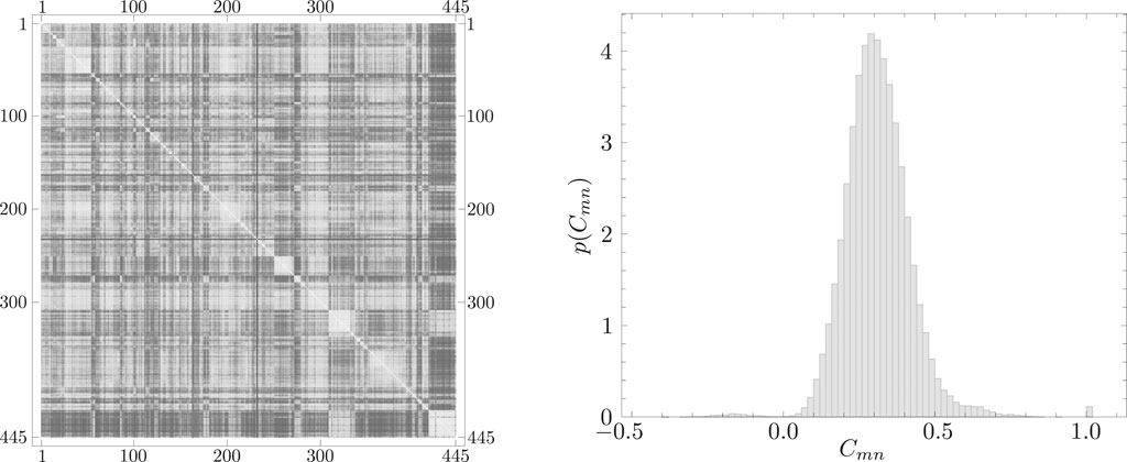
FIGURE 1. (Left) Visualization of the equal-time cross-correlation matrix for the data for 445 assets from S&P 500 from 2010 to 2019 (2,510 business days). The shade is proportional to correlation strength, with white color corresponding to $C_{nn}=1$ and the color becoming dark as the correlation becomes large-magnitude negative. (Right) The distribution $p\left(C_{mn}\right)$ of components of the equal-time cross-correlation matrix. The components are almost all positive. The right tail of the distribution is thicker than the left tail.

2.2 Application of RMT

Calculation of eigenvalues ${\lambda }_R$ for this cross-correlation matrix produces Figure 2. Here, subscript R represents the eigenvalue rankings. The left panel of Figure 2 shows the distribution of eigenvalues. The largest eigenvalue is ${\lambda }_1=143.516$, and the smallest eigenvalue is ${\lambda }_{445}=0.0638128$. The right panel of Figure 2 shows the distribution in the range of small eigenvalues. The solid line is the probability distribution function of the so-called Marčenko-Pastur distribution, which is derived from RMT in the limit $N\to \infty$ and $T\to \infty$ by fixing $Q=N/T$:

$p\left(\lambda \right)={\left(1-\frac{1}{Q}\right)}^{+}\delta \left(\lambda \right)+\frac{1}{2\pi Q}\frac{\sqrt{{\left(\lambda -{\lambda }_{-}\right)}^{+}{\left({\lambda }_{+}-\lambda \right)}^{+}}}{\lambda }(5)$

where ${\left(x\right)}^{+}=\max \left(0,x\right)$; $\delta \left(x\right)$ denotes Dirac’s delta function; and ${\lambda }_{\pm }$ is defined by

${\lambda }_{\pm }={\left(1\pm \sqrt{Q}\right)}^2(6)$

FIGURE 2

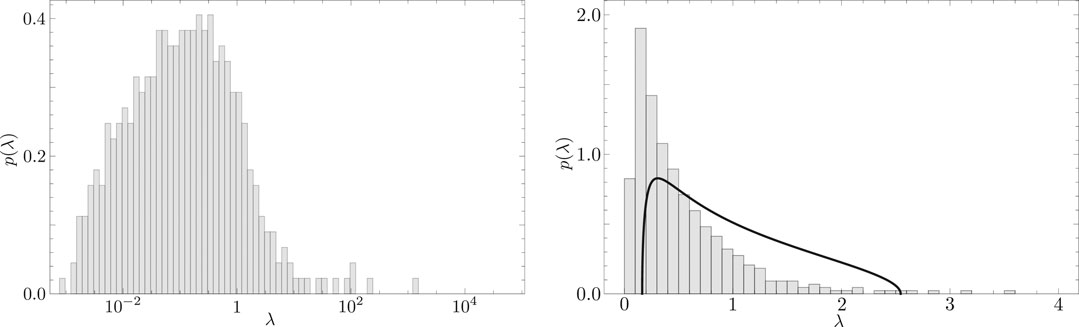
FIGURE 2. (Left) Distribution $p\left(\lambda \right)$ of eigenvalues λ of the empirical equal-time cross-correlation matrix. (Right) Empirically obtained distribution $p\left(\lambda \right)$ of eigenvalues λ in the range of small eigenvalues. The solid line is the Marčenko-Pastur distribution under RMT as the theoretical curve given by Eq. 5.

In this paper, ${\lambda }_{+}=2.01941$ denotes the upper bound of eigenvalue λ, and ${\lambda }_{-}=0.335172$ denotes the lower bound of λ.

In RMT extraction of the meaningful part of the correlation structure, empirical eigenvalues larger than ${\lambda }_{+}$ signify the meaningful part. In particular, in the cross-correlation matrix of stock returns, the largest eigenvalue corresponds to the market mode, and the remaining meaningful part correspond to group modes, such as, industry sectors. In this analysis, it was found that ${\lambda }_1>{\lambda }_2>\dots >{\lambda }_{17}>{\lambda }_{+}$, so, 17 meaningful components were retained.

In traditional PCA, Monte Carlo simulations and so-called scree graphs are used to extract meaningful components. In the present method, the time series of each stock is randomly shuffled to generate an equal-time cross-correlation matrix. This manipulation breaks both the autocorrelation and the cross-correlation. It is derived from a similar concept as the application of RMT. If we construct the equal-time cross-correlation matrix from those randomly shuffled time series, we can obtain the histogram shown in the left panel of Figure 3. The solid line in this figure corresponds to the Marčenko-Pastur distribution given by Eq. 5. From this figure, we can recognize the equivalence between the traditional PCA and the application of RMT.

FIGURE 3

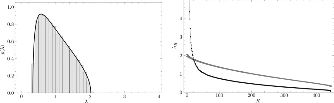
FIGURE 3. (Left) Distribution $p\left(\lambda \right)$ of eigenvalues λ of the equal-time cross-correlation matrix constructed from randomly shuffled time series. The solid line represents the Marčenko-Pastur distribution derived under RMT as the theoretical curve given by Eq. 5. (Right) Scree graph of eigenvalues. The abscissa represents eigenvalue rankings R, and the ordinate represents empirically obtained eigenvalues ${\lambda }_R$. The curve with error bars depicts the simulated distribution of eigenvalues using random shuffling (RS). To obtain this curve, we repeated this manipulation 20 times and calculated the mean value and standard deviation. Each error bar represents three times the standard deviation. The thin line with filled circles depicts the distribution of eigenvalues of the empirical equal-time cross-correlation matrix. The meaningful part can be obtained by comparing these two distributions. If the upper bound for eigenvalues derived from the randomly shuffled cross-correlation matrix is denoted as ${\lambda }_{\max }$, then ${\lambda }_1>{\lambda }_2>\dots >{\lambda }_{19}>{\lambda }_{\max }=1.7947$. Hence, 19 meaningful components should be retained for this data set.

The right panel of Figure 3 shows the scree graph. In this figure, the abscissa corresponds to the eigenvalue rankings and the ordinate corresponds to the magnitude of eigenvalues. The curve with error bars in this figure depicts the eigenvalue distribution of the randomly shuffled cross-correlation matrix. The thin line with filled circles in this figure depicts the distribution of eigenvalues of the empirical equal-time cross-correlation matrix. If we denote the upper bound of eigenvalue derived from the randomly shuffled cross-correlation matrix as ${\lambda }_{\max }$, we obtain ${\lambda }_1>{\lambda }_2>\dots >{\lambda }_{19}>{\lambda }_{\max }=1.7947$. Hence, there are 19 meaningful components in the dataset.

2.3 Application of the RRS

As stated above, when we make a randomly shuffled cross-correlation matrix, we break both the autocorrelation and the cross-correlation conditions. However, it has been reported that the stock price has an autocorrelation tendency. Thus, we need to develop a method that preserves autocorrelation but randomizes the crosscorrelation. [16, 17] developed a method referred to as RRS. In RRS, we shuffle the empirical time-series data rotationally in the time direction and impose the periodic boundary condition:

$w_n\left(t\right)\to w_n\left(Mod\left[t+\tau ,T\right]\right)(7)$

Here, $\tau \in \left[0,T-1\right]$ is a (pseudo-) random integer that is different for each n. For example, if $\tau =1537$ for stock 1, $\tau =2128$ for stock 2, $\dots$, $\tau =138$ for stock N, the time series of normalized log returns is given by

$\begin{array}{l}{w}_1=\left\{w_1\left(1538\right),w_1\left(1539\right),\dots ,w_1\left(2510\right),w_1\left(1\right),w_1\left(2\right),\dots ,w_1\left(1537\right)\right\}\\ w_2=\left\{w_2\left(2129\right),w_2\left(2130\right),\dots ,w_2\left(2510\right),w_2\left(1\right),w_2\left(2\right),\dots ,w_2\left(2128\right)\right\}\\ ⋮⋮\\ w_N=\left\{w_N\left(139\right),w_N\left(140\right),\dots ,w_N\left(2510\right),w_N\left(1\right),w_N\left(2\right),\dots ,w_N\left(138\right)\right\}\end{array}$

Such a rotationally randomly shuffled time series allows the cross-correlation matrix to be constructed and eigenvalues to be calculated. An example is shown in the histogram in the left panel of Figure 4. The solid line in this figure corresponds to the Marčenko-Pastur distribution given by Eq. 5. This figure shows that the distribution of eigenvalues is almost the same as the Marčenko-Pastur distribution based on RMT except for the large eigenvalue range.

FIGURE 4

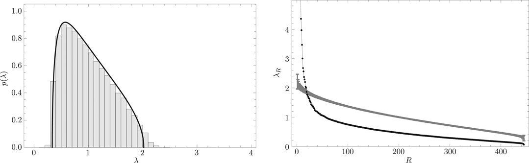
FIGURE 4. (Left) Distribution $p\left(\lambda \right)$ of eigenvalues λ of the equal-time cross-correlation matrix constructed by rotational random shuffling (RRS). The solid line represents the Marčenko-Pastur distribution derived under RMT as the theoretical curve given by Eq. 5. (Right) Scree graph of eigenvalues. The abscissa represents eigenvalue rankings R, and the ordinate represents empirically obtained eigenvalues ${\lambda }_R$. The thin line with filled circles depicts the empirically obtained distribution of eigenvalues of the empirical equal-time cross-correlation matrix. The curve with error bars depicts the simulated distribution of eigenvalues using RRS. To obtain this curve, this manipulation was repeated 20 times, after which the mean value and standard deviation were calculated. Each error bar represents three times the standard deviation. The thin line with filled circles in this figure depicts the distribution of eigenvalues of the empirical equal-time cross-correlation matrix. The meaningful part can be obtained by comparing these two distributions. If the upper bound for eigenvalues derived from the RRS cross-correlation matrix is denoted as ${\lambda }_{\max }$, then ${\lambda }_1>{\lambda }_2>\dots >{\lambda }_{19}>{\lambda }_{\max }=1.7947$. Hence, 19 meaningful components should be retained for this data set.

The right panel of Figure 4 shows the scree graph. In this figure, the abscissa corresponds to eigenvalue rankings, and the ordinate corresponds to eigenvalue magnitude. The curve with error bars in this figure depicts the eigenvalue distribution of the RRS cross-correlation matrix. The thin line with filled circles in this figure depicts the distribution of eigenvalues of the empirical equal-time cross-correlation matrix. Again, if the upper bound of eigenvalues derived from the RRS cross-correlation matrix is denoted as ${\lambda }_{\max }$, then ${\lambda }_1>{\lambda }_2>\dots >{\lambda }_{19}>{\lambda }_{\max }=1.7947$ is obtained. Hence, 19 meaningful components are retained. Although the numbers of meaningful components in RMT and RRS are equal, this result is a coincidence specific to the data set at hand.

Figure 5 shows the distribution of components of the top 20 eigenvectors, $v_1,\dots ,v_{20}$. The thin vertical lines in these figures separate business sectors. RMT suggests that the distribution of the components of each eigenvector is given by the Poter-Thomas distribution:

$p\left(v\right)=\frac{N}{2\pi }\exp \left(-\frac{N{v}^2}{2}\right)(8)$

FIGURE 5

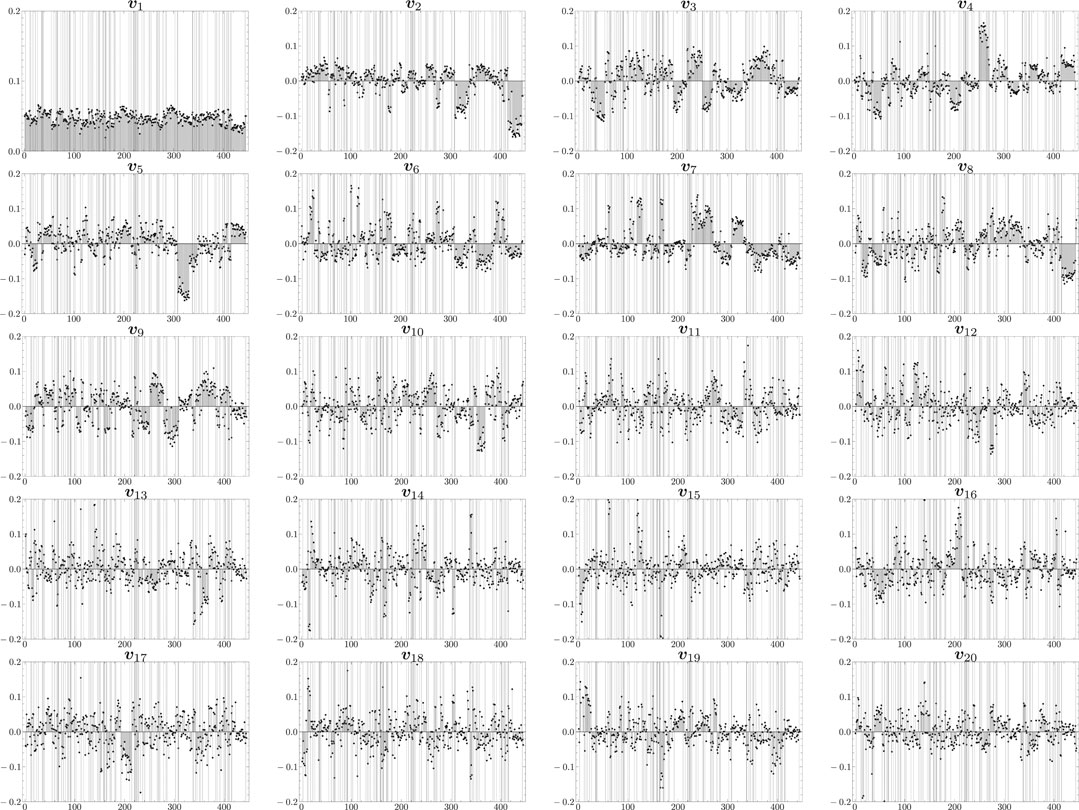
FIGURE 5. Distribution of components of the top 20 eigenvectors, $v_1,\dots ,v_{20}$. The abscissa represents n, and the ordinate represents to the components $v_{R,n}$ of eigenvector $v_R$. Here, R is the eigenvalue rankings. The thin vertical lines in these figures separate business sectors.

The first eigenvector $v_1$ consists of components of similar magnitude and is referred to as the market mode. In the second eigenvector, there is a negative peak in the rightmost sector, which corresponds to the utility sector. In the third eigenvector, there is a negative peak in the left sector, which corresponds to the bank sector. In the fourth eigenvector, there is a positive peak in the middle sector, which corresponds to the oil and gas equipment and service sector. In the fifth eigenvector, there is a negative peak in the right middle sector, which corresponds to the REIT sector. The panels from the sixth eigenvector to the 20th eigenvector have peaks in some sectors containing a small number of assets. However, sometimes it is difficult to extract the meaning of each principal component. Thus, the correlation matrix was split into three parts:

$\begin{array}{l}C={\displaystyle \sum _{R=1}^N{\lambda }_R{v}_R{v}_R^T}\\ ={\lambda }_1{v}_1{v}_1^T+{\displaystyle \sum _{R=2}^{19}{\lambda }_R{v}_R{v}_R^T}+{\displaystyle \sum _{R=20}^N{\lambda }_R{v}_R{v}_R^T}\\ =C_{Market}+C_{Group}+C_{Noise}\end{array}(9)$

It is important to understand why the largest eigenvalue and the corresponding eigenvector are referred to as representing the market mode. The market index on day t is denoted as $w_M\left(t\right)$ and defines it by the scalar product of $w\left(t\right)$ and the first eigenvector $v_1$:

$w_M\left(t\right)=w\left(t\right)\cdot v_1(10)$

i.e., weighting the average return with the weight given by the first eigenvector. On the other hand, the S&P 500 is used to characterize the entire market. The normalized log return on day t from open to close of the S&P 500 is denoted as $w_{SP}\left(t\right)$. Figure 6 shows the scatter plot of $w_M\left(t\right)$ vs. $w_{SP}\left(t\right)$. This figure shows that $w_M\left(t\right)$ and $w_{SP}\left(t\right)$ exhibit a strong, positive correlation. The dashed line in this figure shows a linear function with the slope given by Pearson’s correlation index $\rho =0.852$ and with the intercept equal to 0. This correlation coefficient is almost the same as that obtained by [5].

FIGURE 6

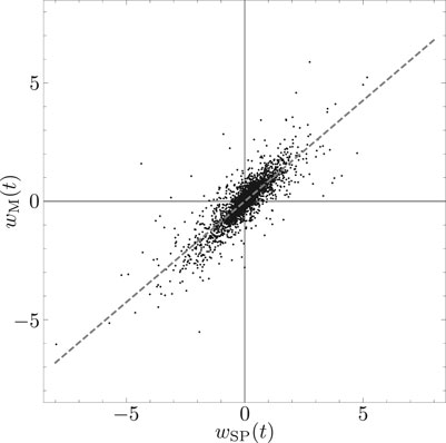
FIGURE 6. Scatter plot of the normalized S&P 500 index $w_{SP}\left(t\right)$ and the normalized market index $w_M\left(t\right)$. The dashed line is linear function with slope ρ, which is Pearson’s correlation index, equal to 0.852, and intercept equal to 0.

3 Application of CHPCA and HHD

In this section, the complex correlation matrix is defined. RRT is then applied to distinguish the meaning components from the noise components, and CHPCA is introduced. After that, HHD is presented in order to clarify the lead-lag relationships among assets.

3.1 Complex Correlation Matrix

A simple definition of different-time correlation is given by $Corr\left[w_m\left(t\right),w_n\left(t+\Delta t\right)\right],\left(\Delta t=1,\dots ,T-1\right)$. However, if N and T are extremely large, a huge number of combinations must be investigated. Therefore, a complex correlation matrix is introduced to overcome this problem.

We consider the Fourier transform of the daily log returns of asset n as represented by

$r_n\left(t\right)={\displaystyle \sum _{k=0}^T\left[a_n\left({\omega }_k\right)\cos \left({\omega }_{k}t\right)+b_n\left({\omega }_k\right)\sin \left({\omega }_{k}t\right)\right]}(11)$

where ${\omega }_k=2\pi k/T\ge 0$. The Hilbert transform of $r_n\left(t\right)$ is given by

${\widehat{r}}_n\left(t\right)={\displaystyle \sum _{k=0}^T\left[b_n\left({\omega }_k\right)\cos \left({\omega }_{k}t\right)-a_n\left({\omega }_k\right)\sin \left({\omega }_{k}t\right)\right]}(12)$

We define a complex log return ${\tilde{r}}_n\left(t\right)$ as

${\tilde{r}}_n\left(t\right)=r_n\left(t\right)+i{\widehat{r}}_n\left(t\right)={\displaystyle \sum _{k=0}^T{c}_n\left({\omega }_k\right)e^{-i{\omega }_{k}t}}(13)$

where i denotes an imaginary unit defined by $i^2=-1$. For each asset n, we define a time average $\langle {\tilde{r}}_n\rangle$ and a standard deviation ${\tilde{\sigma }}_n$ as follows.

$\langle {\tilde{r}}_n\rangle =\frac{1}{T}{\displaystyle \sum _t^T{\tilde{r}}_n\left(t\right)},{\tilde{\sigma }}_n=\sqrt{\frac{1}{T}{\displaystyle \sum _{t=1}^T{\left|{\tilde{r}}_n\left(t\right)-\langle {\tilde{r}}_n\rangle \right|}^2}}(14)$

We define the normalized complex log return ${\tilde{w}}_n\left(t\right)$ as

${\tilde{w}}_n\left(t\right)=\frac{{\tilde{r}}_n\left(t\right)-\langle {\tilde{r}}_n\rangle }{{\tilde{\sigma }}_n}(15)$

Thus, the time-average of ${\tilde{w}}_n\left(t\right)$ is zero, and its standard deviation is one. Each component of the complex correlation matrix is defined by

${\tilde{C}}_{mn}=\frac{1}{T}{\displaystyle \sum _{t=1}^T{\tilde{w}}_m\left(t\right){\tilde{w}}_n^{†}\left(t\right)}(16)$

Herein, $†$ represents the transposed complex conjugate.

The elements of the complex correlation matrix distribute on the complex plane, as shown in the upper left panel of Figure 7. The lower left panel of Figure 7 shows the distribution of the real parts of the elements of the complex correlation matrix. This distribution is almost the same as for the case of the equal-time cross-correlation matrix shown in the right panel of Figure 1. The upper right panel of Figure 7 shows the distribution of the imaginary parts of the elements of the complex correlation matrix. This panel shows a symmetrical distribution.

FIGURE 7

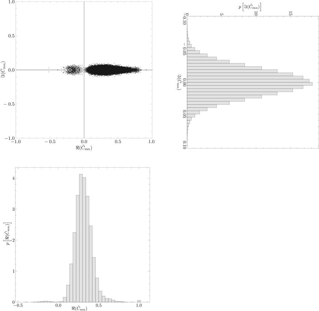
FIGURE 7. (Upper left) Distribution of the elements ${\tilde{C}}_{mn}$ of the complex correlation matrix $\tilde{C}$ in the complex plane $\left[\Re \left({\tilde{C}}_{mn}\right),\Im \left({\tilde{C}}_{mn}\right)\right]$. (Upper right) Distribution $p\left[\Im \left({\tilde{C}}_{mn}\right)\right]$ of the elements of the imaginal part $\Im \left({\tilde{C}}_{mn}\right)$ of the complex correlation matrix. (Lower left) Distribution $p\left[\Re \left({\tilde{C}}_{mn}\right)\right]$ of the elements of the real part $\Re \left({\tilde{C}}_{mn}\right)$ of the complex correlation matrix.

3.2 Complex Hilbert Principal Component Analysis

Figure 8 is obtained by calculating the eigenvalues ${\lambda }_R$ for the cross-correlation matrix. As in Section 2.2, here the subscript R again represents the eigenvalue rankings. The left panel of Figure 8 shows the distribution of the logarithms of eigenvalues. The largest eigenvalue is ${\lambda }_1=143.71$, and the smallest eigenvalue is ${\lambda }_{445}=0.0442842$. The right panel of Figure 8 shows the distribution in the small eigenvalue region. The solid line is the Marčenko-Pastur distribution given by Eq. 5 with $Q=2N/T$.

FIGURE 8

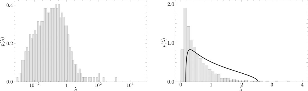
FIGURE 8. (Left) Distribution $p\left(\lambda \right)$ of eigenvalues λ of the empirical equal-time cross-correlation matrix. (Right) Empirically obtained distribution $p\left(\lambda \right)$ of eigenvalues λ in the range of small eigenvalues. The solid line is the Marčenko-Pastur distribution derived under RMT as the theoretical curve given by Eq. 5 with $Q=2N/T$.

Figure 9 shows the scree graph. In this figure, the abscissa corresponds to the eigenvalue rankings and the ordinate corresponds to eigenvalue magnitudes. The curve with error bars in this figure shows the eigenvalue distribution of the RRS complex correlation matrix. The thin line with filled circles in this figure depicts the distribution of eigenvalues of the empirical complex cross-correlation matrix. If we again denote the upper bound for eigenvalues derived from the RRS cross-correlation matrix as ${\lambda }_{\max }$ we again obtain ${\lambda }_1>{\lambda }_2>\dots >{\lambda }_{16}>{\lambda }_{\max }=2.18894$. Hence, 16 meaningful components are retained for this dataset.

FIGURE 9

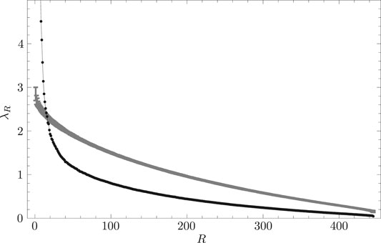
FIGURE 9. Scree graph of eigenvalues. The abscissa represents eigenvalue rankings R, while the ordinate represents empirically obtained eigenvalues ${\lambda }_R$. The curve with error bars in this figure shows the eigenvalue distribution of the RRS complex correlation matrix. To obtain this curve, this manipulation was repeated 20 times, after which the mean value and standard deviation were calculated. Each error bar represents three times the standard deviation. The thin line with filled circles in this figure depicts the distribution of eigenvalues of the empirical equal-time cross-correlation matrix. The meaningful part can be obtained by comparing these two distributions. If the upper bound for eigenvalues derived from the RRS cross-correlation matrix is denoted as ${\lambda }_{\max }$, then ${\lambda }_1>{\lambda }_2>\dots >{\lambda }_{16}>{\lambda }_{\max }=2.18894$. Hence, 16 meaningful components should be retained for this data.

Figure 10 shows the distribution of each component for the top 16 eigenvectors $v_1,\dots ,v_{16}$ in the complex plane. In this case, the Poter-Thomas distribution, which is the null hypothesis of randomness, is given by

$p\left(v\right)=\frac{N}{\pi }\exp \left(-N{\left|v\right|}^2\right)(17)$

FIGURE 10

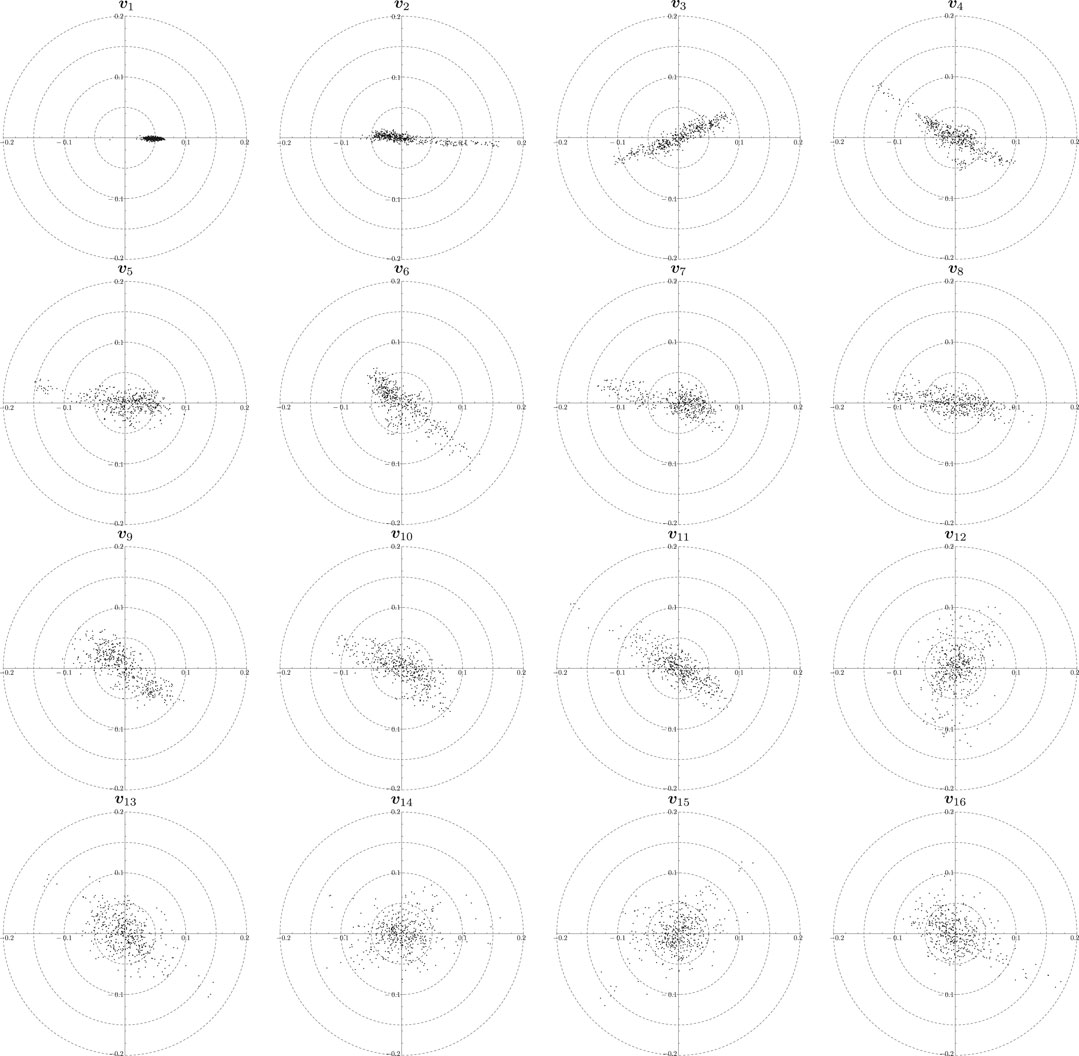
FIGURE 10. Distribution of components of the top 16 eigenvectors, $v_1,\dots ,v_{16}$. In each figure, the abscissa represents $\Re \left(v_{R,n}\right)$, and the ordinate represents $\Im \left(v_{R,n}\right)$. Here, R is the eigenvalue rankings.

In the complex plane, we regard the clockwise direction from the positive real axis as corresponding to leading components, whereas the counterclockwise direction from the positive real axis corresponds to the lagging components. Components of the first eigenvector $v_1$ distribute along the positive real axis. This means that the phase difference, i.e., the difference between leading and lagging, is small for the first eigenvector. Thus, we refer to the first eigenmode as the market mode. On the other hand, components of the 2nd to 16th eigenvectors distribute over a wide region in the complex plane. This behavior suggests group structure.

3.3 Helmholtz-Hodge Decomposition

We decompose the complex correlation matrix into the meaningful part and the noise part as

$\begin{array}{l}\tilde{C}={\displaystyle \sum _{R=1}^N{\lambda }_R{v}_R{v}_R^{†}}\\ ={\displaystyle \sum _{R=1}^{16}{\lambda }_R{v}_R{v}_R^{†}}+{\displaystyle \sum _{R=17}^N{\lambda }_R{v}_R{v}_R^{†}}\\ ={\tilde{C}}_{Principal}+{\tilde{C}}_{Noise}\end{array}(18)$

where $†$ represents taking the complex conjugate of a vector. The left panel of Figure 11 shows the meaningful part of the complex correlation matrix. The introduction of a lower bound for the magnitudes of elements of the principal part of the complex correlation matrix produces, the right panel of Figure 11. The components of the real matrix $F$ are the absolute values of the components of this constrained meaningful correlation matrix. Here, $F$ is considered the weighted adjacency matrix. The components of this matrix can then be written as

$F_{mn}=F_{mn}^{\left(c\right)}+F_{mn}^{\left(p\right)}(19)$

where $F_{mn}^{\left(c\right)}$ corresponds to the circular flow in the network defined by

${\displaystyle \sum _{n=1}^N{F}_{mn}^{\left(c\right)}}=0(20)$

FIGURE 11

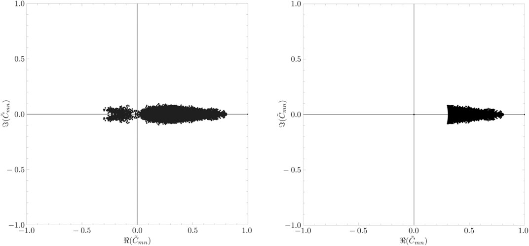
FIGURE 11. (Left) Distribution of the components of the meaningful part of the complex correlation matrix. (Right) Distribution of the components of the constrained meaningful part of the complex correlation matrix.

On the other hand, $F_{mn}^{\left(p\right)}$ corresponds to the gradient flow in the network defined by

$F_{mn}^{\left(p\right)}={\gamma }_{mn}\left({\varphi }_m-{\varphi }_n\right)(21)$

Here, ${\varphi }_m$ is the Helmholtz-Hodge potential. By using Eqs 16, 17 can be rewritten as

${\displaystyle \sum _{n=1}^N\left[F_{mn}-{\gamma }_{mn}\left({\varphi }_m-{\varphi }_n\right)\right]}=0(22)$

By solving Eq. 18, we obtain the Helmholtz-Hodge potential shown in Figure 12. In this figure, the leading components show a small value of the Helmholtz-Hodge potential, while the lagging components show a large value.

FIGURE 12

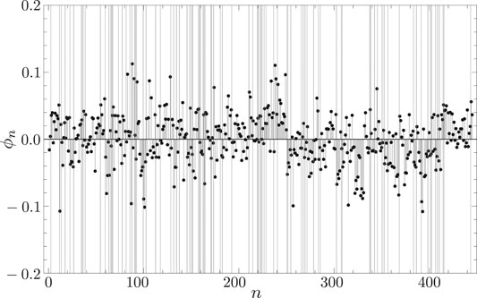
FIGURE 12. Distribution of Helmholtz-Hodge potential for each asset. The abscissa represents n, while the ordinate represents Helmholtz-Hodge potential ${\varphi }_n$. The thin vertical lines in this figure separate business sectors.

The average values $\langle \varphi \rangle$ of the Helmholtz-Hodge potential for some major sectors are shown in Table 1. This table shows that the semiconductors industry is the most strongly leading, while the drug manufacturing industry is the most strongly lagging. On the other hand, [28] explored 483 assets from the S&P 500 for 4-years from 2008 to 2011 (1,009 business days). He obtained the result that the financial sector is the most strongly leading, while the telecommunications and service sector is the most strongly lagging. Therefore, we suspect that the lead-lag structure depends on the gross market conditions of the period investigated. However, clarifying this suspicion is a problem for future study.

TABLE 1

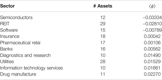
TABLE 1. Helmholtz-Hodge potentials $\langle \varphi \rangle$ for some major business sectors.

4 Application of CHPCA to the Portfolio Theory: A Sketch

As a problem for future study, we consider the application of CHPCA to construct a portfolio by following Markowitz’s portfolio theory [12]. We represent the fraction of wealth invested in asset n as ${\xi }_n$. If we denote the number of assets as K, ${\xi }_n$ is normalized by

${\displaystyle \sum _{n=1}^K{\xi }_n}=1(23)$

By using the complex log return of each asset ${\tilde{r}}_n$ defined by Eq. 9, we define the complex log return of the portfolio ${\tilde{r}}_P$ as

${\tilde{r}}_P={\displaystyle \sum _{n=1}^K{\xi }_n{\tilde{r}}_n}={\displaystyle \sum _{n=1}^K{\xi }_n{r}_n}+i{\displaystyle \sum _{n=1}^K{\xi }_n{\widehat{r}}_n}(24)$

However, the portfolio return must be a real number, so we need to impose the following constraint:

${\displaystyle \sum _{n=1}^K{\xi }_n{\widehat{r}}_n}=0(25)$

The risk of the portfolio is defined by the variance:

$\begin{array}{l}{\tilde{\sigma }}_P^2={\displaystyle \sum _{m=1}^K{\displaystyle \sum _{n=1}^K{\xi }_m{\xi }_n{\tilde{C}}_{mn}{\tilde{\sigma }}_m{\tilde{\sigma }}_n}}\\ ={\displaystyle \sum _{m=1}^K{\displaystyle \sum _{n=1}^K{\xi }_m{\xi }_n\Re \left({\tilde{C}}_{mn}\right){\tilde{\sigma }}_m{\tilde{\sigma }}_n}}+{\displaystyle \sum _{m=1}^K{\displaystyle \sum _{n=1}^K{\xi }_m{\xi }_n\Im \left({\tilde{C}}_{mn}\right){\tilde{\sigma }}_m{\tilde{\sigma }}_n}}\end{array}(26)$

Here again, the risk must be a real number, so we need to impose the following constraint:

${\displaystyle \sum _{m=1}^K{\displaystyle \sum _{n=1}^K{\xi }_m{\xi }_n\Im \left({\tilde{C}}_{mn}\right){\tilde{\sigma }}_m{\tilde{\sigma }}_n}}=0(27)$

Therefore, under the conditions given in Eqs 19, 21, 23, a portfolio can be created that minimizes risk under the assumed returns.

5 Conclusion

An analysis of price data for 445 assets from the S&P 500 from 2010 to 2019 (2,510 business days) provided the basis for an exploration of recent developments in distinguishing the meaningful part from the noise part in correlation structures in big data. Application of RMT to the equal-time cross-correlation matrix was found to be a useful method for obtaining the meaningful components of the correlation structure. However, the null hypothesis of randomness underlying RMT destroyed both real autocorrelation and real cross-correlation in the data. In order to preserve autocorrelation, we introduce RRS. In the case of this paper, the number of meaningful components for RMT and for RRS happened to be. We also introduced CHPCA for investigating the various different-time cross-correlations. By using both CHPCA and HHD, we clarified the lead-lag relationships for some major business sectors.

Data Availability Statement

Publicly available datasets were analyzed in this study. This data can be found here: https://en.wikipedia.org/wiki/List_of_S%26P_500_companies, https://github.com/datasets/s-and-p-500-companies.

Author Contributions

WS wrote this paper by himself.

Funding

This work was supported by JSPS KAKENHI Grant No. JP20228860 and National Bank Academic Research Promotion Foundation in 2019.

Conflict of Interest

The author declares that the research was conducted in the absence of any commercial or financial relationships that could be construed as a potential conflict of interest.

Acknowledgments

The author would like to thank Hiroshi Iyetomi, Hideaki Aoyama, Yoshi Fujiwara, Yuichi Ikeda, Hiroshi Yoshikawa, and Irena Vodenska for useful discussions.

References

1. Laloux L, Cizeau P, Bouchaud J-P, Potters M. Noise dressing of financial correlation matrices. Phys Rev Lett (1999) 83:1467–70. doi:10.1103/physrevlett.83.1467

CrossRef Full Text | Google Scholar

2. Plerou V, Gopikrishnan P, Rosenow B, Nunes Amaral LA, Stanley HE. Universal and nonuniversal properties of cross correlations in financial time series. Phys Rev Lett (1999) 83:1471–4. doi:10.1103/physrevlett.83.1471

CrossRef Full Text | Google Scholar

3. Marčenko VA, Pastur LA. Distribution of eigenvalues for some sets of random matrices. Mathematics USSR-Sbornik (1967) 1:457–83. 10.1070.SM1967v001n04ABEH001994

Google Scholar

4. Porter CE, Thomas RG. Fluctuations of nuclear reaction widths. Phys Rev (1956) 104:483–91. doi:10.1103/physrev.104.483

CrossRef Full Text | Google Scholar

5. Plerou V, Gopikrishnan P, Rosenow B, Amaral LAN, Guhr T, Stanley HE. Random matrix approach to cross correlations in financial data. Phys Rev E, Stat Nonlinear, Soft Matter Phys (2002) 65:066126. doi:10.1103/physreve.65.066126

CrossRef Full Text | Google Scholar

6. Utsugi A, Ino K, Oshikawa M. Random matrix theory analysis of cross correlations in financial markets. Phys Rev E, Stat Nonlinear, Soft Matter Phys (2004) 70:026110. doi:10.1103/physreve.70.026110

CrossRef Full Text | Google Scholar

7. Kim D-H, Jeong H. Systematic analysis of group identification in stock markets. Phys Rev E Stat Nonlinear Soft Matter Phys (2005) 72:046133. doi:10.1103/physreve.72.046133

CrossRef Full Text | Google Scholar

8. Pan RK, Sinha S. Collective behavior of stock price movements in an emerging market. Phys Rev E Stat Nonlinear Soft Matter Phys (2007) 76:046116. doi:10.1103/physreve.76.046116

CrossRef Full Text | Google Scholar

9. Namaki A, Jafari GR, Raei R. Comparing the structure of an emerging market with a mature one under global perturbation. Physica A: Stat Mech its Appl (2011) 390:3020–5. doi:10.1016/j.physa.2011.04.004

CrossRef Full Text | Google Scholar

10. Namaki A, Shirazi AH, Raei R, Jafari GR. Network analysis of a financial market based on genuine correlation and threshold method. Physica A: Stat Mech its Appl (2011) 390:3835–41. doi:10.1016/j.physa.2011.06.033

CrossRef Full Text | Google Scholar

11. Jamali T, Jafari GR. Spectra of empirical autocorrelation matrices: a random-matrix-theory-inspired perspective. EPL (2015) 111:10001. doi:10.1209/0295-5075/111/10001

CrossRef Full Text | Google Scholar

12. Markowitz H. Portfolio selection*. J Finance (1952) 7:77–91. doi:10.1111/j.1540-6261.1952.tb01525.x

CrossRef Full Text | Google Scholar

13. Fujiwara Y, Souma W, Murasato H, Yoon H. Application of PCA and random matrix theory to passive fund management. in: H Takayasua, editors. Practical fruits of econophysics. Berlin, Germany: Springer (2006). p. 226–30.

Google Scholar

14. Souma W. Toward a practical application of econophysics: an approach from random matrix theory (written in Japanese). Appl Math (2005) 15:45–59. doi:10.11540/bjsiam.15.3˙239

CrossRef Full Text | Google Scholar

15. Lo AW, Craig MacKinlay A. An econometric analysis of nonsynchronous trading. J Econom (1990) 45:181–211. doi:10.1016/0304-4076(90)90098-e

CrossRef Full Text | Google Scholar

16. Iyetomi H, Nakayama Y, Aoyama H, Fujiwara Y, Ikeda Y, Souma W. Fluctuation-dissipation theory of input-output interindustrial relations. Phys Rev E Stat Nonlinear Soft Matter Phys (2011a) 83:016103. doi:10.1103/physreve.83.016103

CrossRef Full Text | Google Scholar

17. Iyetomi H, Nakayama Y, Yoshikawa H, Aoyama H, Fujiwara Y, Ikeda Y, et al. What causes business cycles? analysis of the Japanese industrial production data. J Jpn Int Economies (2011) 25:246–72. doi:10.1016/j.jjie.2011.06.002

CrossRef Full Text | Google Scholar

18. Arai Y, Yoshikawa T, Iyetomi H. Complex principal component analysis of dynamic correlations in financial markets. Front Artif Intelligence Appl (2013) 255:111–9. doi:10.3233/978-1-61499-264-6-111

CrossRef Full Text | Google Scholar

19. Arai Y, Yoshikawa T, Iyetomi H. Dynamic stock correlation network. Proced Comp Sci (2015) 60:1826–35. doi:10.1016/j.procs.2015.08.293

CrossRef Full Text | Google Scholar

20. Vodenska I, Aoyama H, Fujiwara Y, Iyetomi H, Arai Y. Interdependencies and causalities in coupled financial networks. PLoS One (2016) 11:e0150994. doi:10.1371/journal.pone.0150994

PubMed Abstract | CrossRef Full Text | Google Scholar

21. Souma W, Aoyama H, Iyetomi H, Fujiwara Y, Vodenska I. Construction and application of new analytical methods for stock correlations: toward the construction of prediction model of the financial crisis (written in Japanese). JWEIN (2016) 1–8.

Google Scholar

22. Souma W, Iyetomi H, Yoshikawa H. Application of complex Hilbert principal component analysis to financial data. in IEEE 41st Annual Computer Software and Applications Conference (COMPSAC); 2017 July 4–8; Turin, Italy. New York, NY: IEEE (2017) 2:391–4.

Google Scholar

23. Souma W, Iyetomi H, Yoshikawa H. The leading and lagging structure of early warning indicators for detecting financial crises (written in Japanese). RIETI Pol Discussion Paper Ser 18-P-005 (2018). p. 1–26.

Google Scholar

24. Kichikawa Y, Iyetomi H, Iino T, Inoue H. Hierarchical and circulating flow structure in an interfirm transaction network. Book of abstracts (2017) 12. Available from: https://core.ac.uk/download/pdf/148338502.pdf#page=27.

Google Scholar

25. Iyetomi H, Ikeda Y, Mizuno T, Ohnishi T, Watanabe T. International trade relationship from a multilateral. Book of abstracts (2017) 253. Available from: https://core.ac.uk/download/pdf/148338502.pdf#page=27.

Google Scholar

26. Kichikawa Y, Iyetomi H, Iino T, Inoue H. Community structure based on circular flow in a large-scale transaction network. Appl Netw Sci (2019) 4:92. doi:10.1007/s41109-019-0202-8

CrossRef Full Text | Google Scholar

27. Iyetomi H, Aoyama H, Fujiwara Y, Souma W, Vodenska I, Yoshikawa H. Relationship between macroeconomic indicators and economic cycles in United States. Scientific Rep (2020) 10:1–12. doi:10.1038/s41598-020-70100-3

CrossRef Full Text | Google Scholar

28. Iyetomi H. Collective phenomena in economic systems. in: H Aoyama, Y Aruka, and H Yoshikawa, editors Complexity, heterogeneity, and the methods of statistical Physics in economics. Berlin, Germany: Springer (2020). p. 177–201.

CrossRef Full Text | Google Scholar