Automated Close-Loop System for Three-Dimensional Characterization of Spatiotemporal Optical Vortex

Recent rapid advances in spatiotemporal optical pulses demand accurate characterization of the spatiotemporal structure of the produced light fields. We report an automated close-loop characterization system that is capable of reconstructing the three-dimensional intensity and phase structures of spatiotemporal wavepacket illustrated by characterizing spatiotemporal optical vortex in the spatiotemporal domain. The characterization technique is based on interfering a much shorter probe pulse with different slices of the object wavepacket along the temporal axis. A close-loop control program is developed to realize full automation of the data collection and reconstruction process. Experimental results of the intensity and phase distributions show that the designed close-loop system is efficient in quantitatively characterizing the generated spatiotemporal optical vortex. Such a linear characterization system can also be extended to measure many other kinds of spatiotemporal wavepacket and may find broad applications in spatiotemporal wavepacket studies.

1 Introduction

Optical vortex beam carrying orbital angular momentum (OAM) is widely known as a beam with phase singularity caused by a spiral wavefront [1–3]. In 1992, Allen et al. recognized that the special helical phase for a vortex beam could be expressed as $\mathit{exp}\left(il\theta \right)$, where l is the topological charge and θ is the azimuthal angle [4]. In the same year, Bazhenov et al. obtained controllable vortex beams by using diffraction on computer-synthesized gratings [5]. Owing to its unique properties, vortex beams have been widely studied and applied in many fields, such as particle manipulation [6–8], free-space optical communication [9–12], quantum information encoding [13], optical measurement [14], super-resolution imaging [15, 16], and laser processing and material processing [17].

Many methods have been developed to generate OAM beams. Such beams carrying photons with discrete OAM are readily realizable in the laboratory nowadays. For example, a reconfigurable spiral phase plate was proposed to create optical vortices with tunable operating wavelengths and topological charges [18]. Moreover, a fiber structure of a square core and ring refractive index profile had been demonstrated to convert the circular polarized Gaussian modes into optical OAM modes. By breaking the circular symmetry of the waveguide, the circular polarized fundamental modes in the square core could be coupled into the ring region to generate higher-order OAM modes through the transference of spin angular momentum and OAM [19]. Furthermore, the effective indices of an optical fiber had been designed for maximal separation of each vector mode, facilitating the use of OAM modes for space-division multiplexing. This kind of fiber could support up to 16 OAM modes [20]. In addition, liquid crystal spatial light modulator (SLM) has been commonly used in the generation of vortex beam [21]. An optical vortex array with controllable size and quantity had been created by employing a simple optical system based on SLM and mode converter [22]. An optical vortex whose dark hollow radius did not depend on the topological charge could be obtained in the Fourier transforming optical system with a computer-controlled liquid-crystal SLM [23]. The deformations caused by transmissive SLMs with nonlinear and incomplete phase modulation could be corrected by modifying the numerical optimization coherent phase diversity to improve on-axis optical vortex generation [24]. These traditional OAM can be measured by adopting the interference and diffraction properties of optical vortex [25].

The longitudinal OAM will lead to the electromagnetic energy of vortex beam circulating around an axis parallel to the propagation direction of the beam, as shown in Figure 1A, whereas transverse OAM will make the vortex circulate around an axis perpendicular to the propagation direction of the beam, as shown in Figure 1B. Most studies have been focused on the longitudinal OAM, while few literatures have been reported on the transverse OAM. Recent theoretical studies indicated that transverse OAM could be formed by introducing the temporal variations of the phase [26], that is, creating the spatiotemporal optical vortex (STOV). An optical field with a small fraction of the energy exhibits the transverse OAM via a nonlinear interaction between an extremely high-power pulse and air [27]. More recently, based on high-resolution SLMs, a linear method that could experimentally produce STOV with pure transverse OAM in a controllable manner was reported [28]. Spatiotemporal (ST) wavepacket can be pre-conditioned to overcome the ST astigmatism in the strong focusing, leading to the creation of STOV with sub-wavelength transverse sizes [29]. STOV offers new opportunities for controlling pulsed optical beams, which are expected to open many important applications that exploit the interactions of such ST wavepackets with matters. Accurate three-dimensional (3D) characterization of STOV is crucial for further studies of this kind of novel ST wavepackets. In this article, we present a close-loop characterization system that is capable of reconstructing the 3D intensity structure of STOV in ST domain and extracting its ST helical phase simultaneously. This linear characterization technique is based on the interference of a much shorter compressed probe pulse with the ST wavepacket to be characterized. Time delay of the probe pulse is adjusted by an electronically controlled translation stage to make the probe pulse interfere with the different slice of object wavepacket along the temporal axis. Control program based on National Instruments LabVIEW is developed to achieve automatic scan throughout the object wavepacket as well as data processing after all the interference patterns are collected.

FIGURE 1

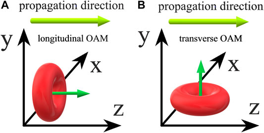
FIGURE 1. Comparison of vortex beams with longitudinal OAM (A) and transverse OAM (B). OAM, orbital angular momentum.

2 Linear Characterization of Spatiotemporal Optical Vortex

2.1 Three-Dimensional Reconstruction Principle

The three-dimensional reconstruction method is based on a noncollinear first-order cross-correlation [30–33]. This linear optical approach is simple to implement and suitable for the measurement of many kinds of pulses. The principle of this method is illustrated in Figure 2. A laser pulse is divided into two pulses, as shown in Figure 2A. One of them is directed to the pulse-shaping setup to generate the object wavepacket. The other is compressed to form an ultrashort pulse to act as a probe pulse. The probe pulse then interferes with the object wavepacket at different time slices, as shown in Figure 2B. The time delay of the object wavepacket slice is controlled by an electronically controlled translation stage.

FIGURE 2

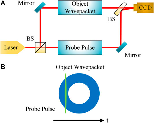
FIGURE 2. Three-dimensional reconstruction principle of object wavepacket. BS, beam splitter.

The intensity of the interference pattern collected by the CCD camera can be expressed as:

$I\left(\tau ,\overrightarrow{r}\right)\approx I_o\left(\overrightarrow{r}\right)+I_p\left(\overrightarrow{r}\right)+2\cos \left(\omega \left[\tau +\delta \left(\overrightarrow{r}\right)\right]\right)\times \sqrt{△t_p{i}_o}\left(\tau ,\overrightarrow{r}\right)\sqrt{I_p\left(\overrightarrow{r}\right)}(1)$

where $I_o\left(\overrightarrow{r}\right)$ is the intensity of the object wavepacket, $I_p\left(\overrightarrow{r}\right)$ is the intensity of the probe pulse, ω is the angular frequency of the laser pulse, τ is the time delay of the object wavepacket slice, $\overrightarrow{r}$ refers to the spatial domain $\left(x,y,z\right)$, and $\delta \left(\overrightarrow{r}\right)$ is the additional location-dependent delay due to the angle between the two pulses. $\Delta t_p$ is the duration of the probe pulse, and $i_o\left(\tau ,\overrightarrow{r}\right)$ is the object pulse intensity at different time slices. It can be found that $i_o\left(\tau ,\overrightarrow{r}\right)$ is proportional to $P^2\left(\tau ,\overrightarrow{r}\right)/I_p\left(\overrightarrow{r}\right)$, as shown in the following equation:

$i_o\left(\tau ,\overrightarrow{r}\right)=\frac{P^2\left(\tau ,\overrightarrow{r}\right)}{I_p\left(\overrightarrow{r}\right)}(2)$

where $P\left(\tau ,\overrightarrow{r}\right)$ is the amplitude of the coupling term in Eq 1, which can be given by

$P\left(\tau ,\overrightarrow{r}\right)=\frac{I\left(\tau ,\overrightarrow{r}\right)-I_o\left(\overrightarrow{r}\right)-I_p\left(\overrightarrow{r}\right)}{2\cos \left(\omega \left(\tau +\delta \left(\overrightarrow{r}\right)\right)\right)\times \sqrt{\Delta t_p}}(3)$

In each measurement, we need to obtain the intensities of the object wavepacket, the probe pulse, and the interference term. Since the object wavepacket intensity $I_o\left(\overrightarrow{r}\right)$ and the probe pulse intensity $I_p\left(\overrightarrow{r}\right)$ will remain nearly unchanged throughout the whole measurement, these two intensities just need to be measured once. Therefore, we only need to measure the intensity of the interference pattern $I\left(\tau ,\overrightarrow{r}\right)$ at each time delay. We can extract both the intensity and phase distributions from $i_o\left(\tau ,\overrightarrow{r}\right)$ (more details can be found in Ref. [30]). Here, we also measured the background beam $I_B\left(\overrightarrow{r}\right)$ to filter out the ambient noise. Finally, we can reconstruct the 3D ST structure of an STOV by stitching the intensity and phase of each time slice, which are obtained by processing the corresponding experimental data.

2.2 Pulsed Laser Source

In the experimental setup, a ytterbium (Yb)-doped fiber laser pumped by a 980-nm laser diode (Thorlabs BL976-PAG900) is adopted as the light source [34]. As shown in Figure 3, the pump beam is delivered to the gain fiber by a wavelength division multiplexing coupler. The diffraction grating pair is exploited to compensate the normal group velocity dispersion of the fiber. Mode-locked operation is achieved through nonlinear polarization evolution (NPE), which is implemented with the quarter waveplates and half waveplates. The 1030-nm pulse beam is taken directly from the NPE ejection port, namely reflected by the polarization beam splitter (BS).

FIGURE 3

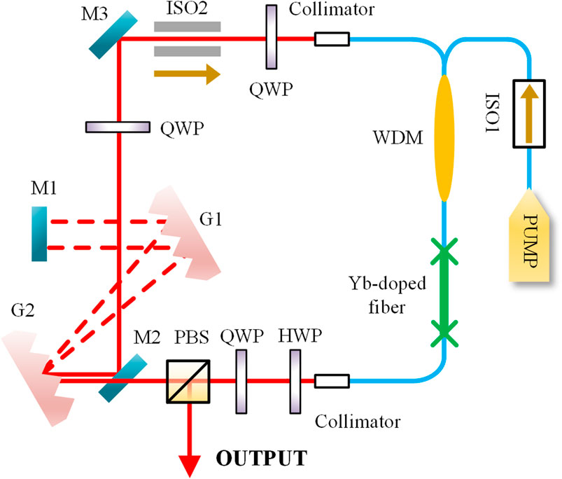
FIGURE 3. Fiber laser. G, grating; M, mirror; ISO, isolator; PBS, polarization beam splitter; PUMP, pump source; QWP, quarter waveplate; HWP, half waveplate; WDM, wavelength division multiplexer.

2.3 Automatic Characterization Setup

The experimental setup for the generation and automatic characterization of the STOV is shown in Figure 4. The pulse beam with about 3 ps duration from fiber laser is first expanded by beam expander (BE) 1 and then splitted into two pulses by nonpolarizing BS1. One of them is directed to the pulse shaper to generate the STOV [28], which acts as the object wavepacket. The pulse shaper consists of the diffraction grating 1 (G1), cylindrical lens, and the SLM. In the pulse shaper, the G1 and the cylindrical lens will perform a time-to-frequency Fourier transformation on the incident chirped mode-locked pulses. Subsequently, a spiral phase on the SLM is displayed to the transformed wavepacket in the spatial frequency–frequency domain ($k_x-\omega$ plane). Then, the reflected wavepacket from the SLM passes through the same grating–cylindrical lens pair, which conducts an inverse Fourier transformation from the $k_x-\omega$ plane to the spatial-temporal domain ($x-t$ plane). The spiral phase will be conserved after the inverse Fourier transformation, forming a chirped STOV.

FIGURE 4

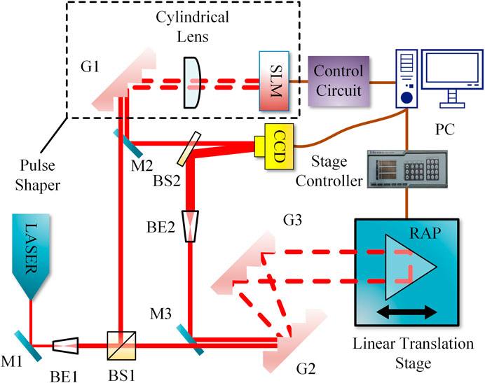
FIGURE 4. Experimental setup for the automatic characterization of the STOV. G, grating; M, mirror; BS, beam splitter; RAP, right angular prism; PC, personal computer; Linear translation stage: one-dimensional electronically controlled translation stage; SLM, spatial light modulator; BE, beam expander; LASER, pulsed laser source.

The other pulse is used as the probe after it is compressed by a parallel grating pair to about 90 fs. A right angular prism serving as retro-reflector is fixed on a linear translation stage (Zolix MAR20-65) to function as a computer-controlled time delay line. Then, the probe pulse is expanded by BE2 and directed to CCD by BS2, which overlaps with the object wavepacket at a small angle to form interference fringes. The scan throughout the object wavepacket is automatically performed by a control program based on LabVIEW.

2.4 Control Program

Hundreds of interference patterns need to be collected to reconstruct the 3D ST structure of STOV, with one interference pattern captured for each position of the linear stage. Manual collection and processing will be tedious and inaccurate. Therefore, a program is developed to execute this process automatically. An automated program not only can reduce the measurement time but also increase the accuracy of collected data.

In our experimental setup, the SC300-1A controller is used to control the stage with minimum incremental motion of $2\text{μm}$, and the Ophir Optronics BeamGage software is employed to control the CCD camera for data acquisition. Both of them are controlled by LabVIEW program and can be combined together to achieve close-loop control. Meanwhile, calling MathWorks MATLAB program is also integrated in LabVIEW control program for data processing.

The function modules in the program to establish the connection with the stage and BeamGage are shown in Figure 5. The commands in Figure 5A are used to connect the corresponding port to open the stage. Since the stage moves over a very short distance in the experiments, the parameter ‘pitch’ of the stage should be set to 1 when the stage is started to ensure the displacement precision of the stage. Commands in Figure 5B are utilized to start BeamGage software to control the CCD and set its configuration. The commands in Figure 6A are used for moving the stage, and the commands in Figure 6B are employed to export the interference fringes data collected by CCD in the corresponding format.

FIGURE 5

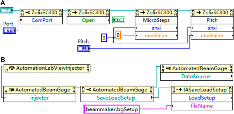
FIGURE 5. Function modules in the control program to establish the connection with the stage (A) and BeamGage (B).

FIGURE 6

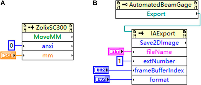
FIGURE 6. Function modules to control stage (A) and CCD (B) in data acquisition.

Based on the two modules in Figure 6, we can build up a state machine used for automatic data acquisition, which is the kernel of the close-loop control program. The block diagram of state transfer and LabVIEW program for the state machine are shown in Figures 7A,B, respectively. First, the BeamGage acquisition commands are called to put CCD into working state. Then, commands in Figure 6A are called to move the stage with specified displacement. After that, the state machine is suspended to wait for 2 s to stabilize the interference fringes captured by the CCD. Subsequently, CCD is paused by calling the stop command of BeamGage in the LabVIEW program. Next, the commands in Figure 6B are called twice to export the data of the captured interference pattern in both JPEG and ASCII formats. The JPEG image is used for directly viewing the saved interference pattern, while the ASCII file is for data processing. Afterward, the state machine puts the CCD into work again. The above state transfer will be repeated many times until the scan of the STOV to be measured is finished. By using the state machines, we can both improve the stability of the close-loop control program and enable instant stop at any state during the operation of the program.

FIGURE 7

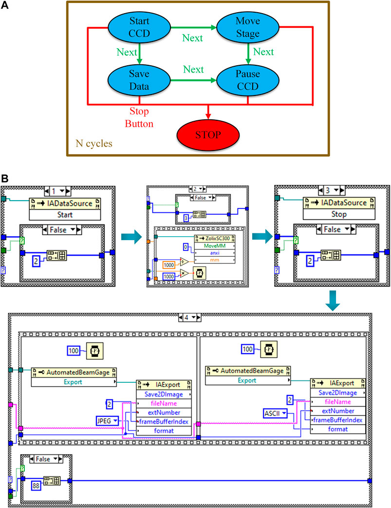
FIGURE 7. State machine for automatic data acquisition. (A) Block diagram of state transfer, N cycles are required for scan throughout the STOV to be measured and (B) LabVIEW program for State machine.

Integration of the aforementioned functional modules establishes the close-loop control program for automatic data acquisition. The program flowchart is shown in Figure 8, and the corresponding graphical user interface is shown in Figure 9. When the program is started, the CCD will be turned on automatically. After that, the program will enter standby mode and wait for the next command. At this time, one can choose to execute any of the following instructions: save the current captured data (‘Save’ button in the ‘Data acquisition and processing’ panel), open the stage (‘Open Stage’ button in the ‘Control’ panel), or close the CCD (‘Close CCD’ button in the ‘Control’ panel). When the stage is opened, the stage can be moved by the ‘+’ and ‘–’ buttons with the input displacement. Meanwhile, the stage can also be set to desired parameters with ‘Setting’ button. In the ‘Data acquisition and processing’ panel, we can set the movement step of the stage, delay after movement, name of the saved file in each collection, and sample times needed to scan through the entire STOV. Then we can press the ‘Startup’ button to launch the state machine for automatic data acquisition. During the acquisition, all the buttons are disabled except the ‘Stop’ button, which is designed to abort the state machine in an emergency. Finally, we can press the ‘3D Reconstruction’ button to process the collected data, extracting the phase distribution in the ST domain and reconstructing the 3D ST wavepacket.

FIGURE 8

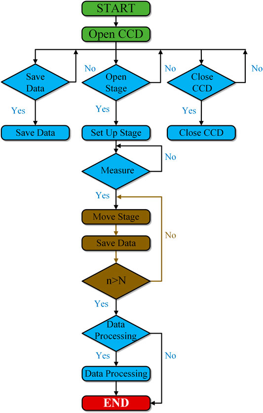
FIGURE 8. Flowchart of the automated control program.

FIGURE 9

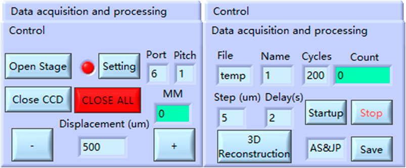
FIGURE 9. Graphical user interface for the automated control program.

3 Experimental Results

To illustrate the capability of the system, we apply a spiral phase of topological charge of 1 to the laser pulse in the spatial frequency–frequency domain through the SLM in the pulse shaper as an example [28]. The movement step of the stage is set to $5\text{μm}$. Based on the close-loop characterization system, about 200 frames of interference patterns are automatically collected by the CCD to scan through the generated ST wavepacket along the t-axis. Several typical interference fringes among the collected data are shown in Figure 10A. The first and fifth interference patterns are obtained near the beginning and end of the ST wavepacket, respectively. Obviously, the upper and lower fringes in each of them are almost aligned, indicating the phase difference between the upper and lower parts in each slice of the generated ST wavepacket is close to zero. The second and fourth interference patterns are captured at both sides near the center of the ST wavepacket, respectively. It is clear that the orientations of the misalignment between the upper and lower fringes are opposite in these two patterns. Hence, there exists phase difference between the upper and lower parts in each slice, and the phase differences in these two patterns are opposite. The third interference pattern is collected at the center of the ST wavepacket. The complete misalignment between the upper and lower fringes reveals that the phase difference between the upper and lower parts of this slice is about π.

FIGURE 10

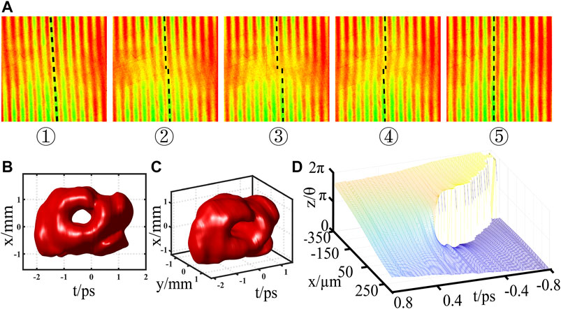
FIGURE 10. Characterization results of STOV with topological charge 1. (A) Experimentally measured interference fringes, (B) front view of the reconstructed 3D STOV, (C) side view of the reconstructed 3D STOV, and (D) extracted phase distribution in the ST domain.

With all the measured data, we can reconstruct the 3D structure of the ST wavepacket, as shown in Figures 10B,C. The reconstructed 3D ST wavepacket is depicted by isosurface at 15% of its maximum intensity, from which we can see a donut shape with hollow core in the $x-t$ plane. These two figures show the same reconstructed wavepacket at different view angles. Obviously, the experimental results are consistent with the simulation results in Figures 11A,B. The extracted ST phase distribution of the generated wavepacket is demonstrated in Figure 10D. Clearly, the phase varies from 0 to $2\text{π}$ in the ST domain, revealing the wavepacket carries ST OAM with topological charge of 1. The experimentally measured phase distribution is also consistent with the simulation result in Figure 11C. The measured results are slightly different from the simulation results. The simulation is based on an ideal assumption of the beam profiles in both spatial and temporal domain with perfect spiral phase modulation in the ST domain. However, in practice, the phase modulation error of the SLM, measurement error of the CCD, step resolution of linear translation stage, pulse width of the probe beam, actual pulse shape from the fiber laser, etc., will all deviate from the ideal situation. However, the key features of the reconstructed STOV agree well with the simulation results, namely, there exist hollow centers caused by phase singularity in both the experimentally reconstructed and theoretical 3D wavepacket in the $x-t$ domain. Meanwhile, both of the corresponding ST spiral phase distributions change from 0 to $2\text{π}$. To improve the accuracy of the measurement, we may further compress the pulse width of the probe beam, adjust the mode lock of the fiber laser to regulate the pulse shape along the time domain, optimize the phase modulation precision of the SLM, adopt translation stage with higher step resolution, and employ CCD with higher dynamic range. Hereby, we obtain both the 3D structure of the experimentally generated STOV and its ST helical phase, demonstrating the effectiveness of the close-loop characterization system in automatic data acquisition and process.

FIGURE 11

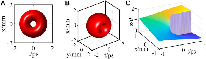
FIGURE 11. Simulation results of STOV with topological charge 1. (A) Front view of 3D STOV, (B) side view of 3D STOV, and (C) phase distribution.

4 Conclusion

In conclusion, we demonstrate an automated close-loop characterization system to reconstruct the 3D wavepacket of experimentally generated STOV and extract its ST helical phase. One pulse divided from the picosecond pulse laser is directed into the pulse shaper to create the STOV as the object wavepacket, while the other pulse is compressed to serve as the probe pulse. The time delay of the probe pulse is adjusted by an electronically controlled translation stage to make the probe pulse interfere with the different slice of object wavepacket along the time axis. A control program is developed to achieve the automatic scan through the object wavepacket and automatic data processing. STOV with topological charge of 1 in the ST domain is experimentally generated; 200 samples are automatically collected by employing the automatic characterization system. The reconstruction results show that the presented close-loop system is efficient in quantitatively characterizing both the 3D ST intensity and phase distributions of the generated STOV. Although the capability of this linear characterization method is demonstrated with STOV, this method can be extended to wavepackets with more general ST distributions, paving the way to further studies in this nascent field that may inspire a myriad of applications ranging from microscopy, plasma physics, laser machining, to quantum information processing.

Data Availability Statement

The raw data supporting the conclusions of this article will be made available by the authors, without undue reservation.

Author Contributions

JC proposed the idea. JC and KL performed the research and built the control system. QC, HH, and CW gave suggestions in data processing. QZ supervised the project. All authors contributed to the revision of the manuscript and approved the submitted version.

Funding

This work was supported by the National Natural Science Foundation of China (grant nos. 92050202, 61805142, 62075132, and 61875245); the Shanghai Science and Technology Committee (grant no. 19060502500), and the Natural Science Foundation of Shanghai (grant no. 20ZR1437600).

Conflict of Interest

The authors declare that the research was conducted in the absence of any commercial or financial relationships that could be construed as a potential conflict of interest.

References

1. Harwit M. Photon orbital angular momentum in astrophysics. Astrophysical J (2003) 597:1266. doi:10.1086/378623

CrossRef Full Text | Google Scholar

2. Mair A, Vaziri A, Weihs G, Zeilinger A. Entanglement of the orbital angular momentum states of photons. Nature (2001) 412:313–6. doi:10.1038/35085529

PubMed Abstract | CrossRef Full Text | Google Scholar

3. O’Neil AT, MacVicar I, Allen L, Padgett MJ. Intrinsic and extrinsic nature of the orbital angular momentum of a light beam. Phys Rev Lett (2002) 88:053601. doi:10.1103/PhysRevLett.88.053601

PubMed Abstract | CrossRef Full Text | Google Scholar

4. Allen L, Beijersbergen MW, Spreeuw R, Woerdman J. Orbital angular momentum of light and the transformation of laguerre-gaussian laser modes. Phys Rev A (1992) 45:8185. doi:10.1103/physreva.45.8185

PubMed Abstract | CrossRef Full Text | Google Scholar

5. Bazhenov VY, Soskin MS, Vasnetsov MV. Screw dislocations in light wavefronts. J Mod Opt (1992) 39:985–90. doi:10.1080/09500349214551011

CrossRef Full Text | Google Scholar

6. Ashkin A, Dziedzic JM, Bjorkholm JE, Chu S. Observation of a single-beam gradient force optical trap for dielectric particles. Opt Lett (1986) 11:288–90. doi:10.1364/ol.11.000288

PubMed Abstract | CrossRef Full Text | Google Scholar

7. Curtis JE, Koss BA, Grier DG. Dynamic holographic optical tweezers. Opt Commun (2002) 207:169–75. doi:10.1016/s0030-4018(02)01524-9

CrossRef Full Text | Google Scholar

8. La Porta A, Wang MD. Optical torque wrench: angular trapping, rotation, and torque detection of quartz microparticles. Phys Rev Lett (2004) 92:190801. doi:10.1103/physrevlett.92.190801

PubMed Abstract | CrossRef Full Text | Google Scholar

9. Djordjevic IB, Arabaci M. Ldpc-coded orbital angular momentum (oam) modulation for free-space optical communication. Opt Express (2010) 18:24722–8. doi:10.1364/oe.18.024722

PubMed Abstract | CrossRef Full Text | Google Scholar

10. Wang J, Yang J-Y, Fazal IM, Ahmed N, Yan Y, Huang H, et al. Terabit free-space data transmission employing orbital angular momentum multiplexing. Nat Photon (2012) 6:488–96. doi:10.1038/nphoton.2012.138

CrossRef Full Text | Google Scholar

11. Wang Z, Zhang N, Yuan X-C. High-volume optical vortex multiplexing and de-multiplexing for free-space optical communication. Opt Express (2011) 19:482–92. doi:10.1364/oe.19.000482

PubMed Abstract | CrossRef Full Text | Google Scholar

12. Zhu J, Zhu K, Tang H, Xia H. Average intensity and spreading of an astigmatic sinh-gaussian beam with small beam width propagating in atmospheric turbulence. J Mod Opt (2017) 64:1915–21. doi:10.1080/09500340.2017.1326638

CrossRef Full Text | Google Scholar

13. Vaziri A, Pan J.-W, Jennewein T, Weihs G, Zeilinger A. Concentration of higher dimensional entanglement: qutrits of photon orbital angular momentum. Phys Rev Lett (2003) 91:227902. doi:10.1103/physrevlett.91.227902

PubMed Abstract | CrossRef Full Text | Google Scholar

14. Lavery MPJ, Speirits FC, Barnett SM, Padgett MJ. Detection of a spinning object using light’s orbital angular momentum. Science (2013) 341:537–40. doi:10.1126/science.1239936

PubMed Abstract | CrossRef Full Text | Google Scholar

15. Yan L, Gregg P, Karimi E, Rubano A, Marrucci L, Boyd R, et al. Q-plate enabled spectrally diverse orbital-angular-momentum conversion for stimulated emission depletion microscopy. Optica (2015) 2(10):900–3. doi:10.1364/OPTICA.2.000900

16. Tamburini F, Anzolin G, Umbriaco G, Bianchini A, Barbieri C. Overcoming the Rayleigh criterion limit with optical vortices. Phys Rev Lett (2006) 97(16):163903. doi:10.1103/PhysRevLett.97.163903

17. Allegre OJ, Jin Y, Perrie W, Ouyang J, Fearon E, Edwardson SP, et al. Complete wavefront and polarization control for ultrashort-pulse laser microprocessing. Opt Express (2013) 21:21198–207. doi:10.1364/oe.21.021198

PubMed Abstract | CrossRef Full Text | Google Scholar

18. Algorri JF, Urruchi V, Garcia-Cámara B, Sánchez-Pena JM. Generation of optical vortices by an ideal liquid crystal spiral phase plate. IEEE Electron Device Lett (2014) 35:856–8. doi:10.1109/led.2014.2331339

CrossRef Full Text | Google Scholar

19. Yan Y, Zhang L, Wang J, Yang J-Y, Fazal IM, Ahmed N, et al. Fiber structure to convert a gaussian beam to higher-order optical orbital angular momentum modes. Opt. Lett. (2012) 37:3294–6. doi:10.1364/ol.37.003294

PubMed Abstract | CrossRef Full Text | Google Scholar

20. Brunet C, Ung B, Messaddeq Y, LaRochelle S, Bernier E, Rusch LA. Design of an optical fiber supporting 16 oam modes. In: Optical Fiber Communication Conference; 2014 Mar 9–Mar 14; San Francisco, CA, United States. IEEE (2014). p. Th2A–24. doi:10.1364/OFC.2014.Th2A.24

Google Scholar

21. Kumar A, Vaity P, Bhatt J, Singh RP. Stability of higher order optical vortices produced by spatial light modulators. J Mod Opt (2013) 60:1696–700. doi:10.1080/09500340.2013.852696

CrossRef Full Text | Google Scholar

22. Huang TD, Lu TH. Controlling an optical vortex array from a vortex phase plate, mode converter, and spatial light modulator. Opt Lett (2019) 44:3917–20. doi:10.1364/ol.44.003917

PubMed Abstract | CrossRef Full Text | Google Scholar

23. Ostrovsky AS, Rickenstorff-Parrao C, Arrizón V. Generation of the “perfect” optical vortex using a liquid-crystal spatial light modulator. Opt Lett (2013) 38:534–6. doi:10.1364/ol.38.000534

PubMed Abstract | CrossRef Full Text | Google Scholar

24. Cuartas-Vélez C, Restrepo R, Echeverri-Chación S, Uribe-Patarroyo N. Improving on-axis optical vortex generation by transmissive spatial light modulator using coherent phase diversity. In: Latin America Optics and Photonics Conference; 2016 Aug 22–Aug 26; Medellin, Colombia. Optical Society of America (2016). p. LW3D.4. doi:10.1364/LAOP.2016.LW3D.4

Google Scholar

25. Shen Y, Wang X, Xie Z, Min C, Fu X, Liu Q, et al. Optical vortices 30 years on: Oam manipulation from topological charge to multiple singularities. Light: Sci Appl (2019) 8:1–29. doi:10.1038/s41377-019-0194-2

PubMed Abstract | CrossRef Full Text | Google Scholar

26. Bliokh KY, Nori F. Spatiotemporal vortex beams and angular momentum. Phys Rev A (2012) 86:033824. doi:10.1103/physreva.86.033824

CrossRef Full Text | Google Scholar

27. Jhajj N, Larkin I, Rosenthal E, Zahedpour S, Wahlstrand J, Milchberg H. Spatiotemporal optical vortices. Phys Rev X (2016) 6:031037. doi:10.1103/physrevx.6.031037

CrossRef Full Text | Google Scholar

28. Chong A, Wan C, Chen J, Zhan Q. Generation of spatiotemporal optical vortices with controllable transverse orbital angular momentum. Nat Photon (2020) 14:350–4. doi:10.1038/s41566-020-0587-z

CrossRef Full Text | Google Scholar

29. Chen J, Wan C, Chong A, Zhan Q. Subwavelength focusing of a spatio-temporal wave packet with transverse orbital angular momentum. Opt Express (2020) 28:18472–8. doi:10.1364/oe.394428

PubMed Abstract | CrossRef Full Text | Google Scholar

30. Li H, Bazarov IV, Dunham BM, Wise FW. Three-dimensional laser pulse intensity diagnostic for photoinjectors. Phys Rev Spec Topics-Accelerators Beams (2011) 14:112802. doi:10.1103/physrevstab.14.112802

CrossRef Full Text | Google Scholar

31. Li Y, Chemerisov S. Manipulation of spatiotemporal photon distribution via chromatic aberration. Opt Lett (2008) 33:1996–8. doi:10.1364/ol.33.001996

PubMed Abstract | CrossRef Full Text | Google Scholar

32. Li Y, Chemerisov S, Lewellen J. Laser pulse shaping for generating uniform three-dimensional ellipsoidal electron beams. Phys Rev Spec Topics-Accelerators Beams (2009) 12:020702. doi:10.1103/physrevstab.12.020702

CrossRef Full Text | Google Scholar

33. Li Y, Lewellen JW. Generating a quasiellipsoidal electron beam by 3d laser-pulse shaping. Phys Rev Lett (2008) 100:074801. doi:10.1103/physrevlett.100.074801

PubMed Abstract | CrossRef Full Text | Google Scholar

34. Lim H, Ilday FO, Wise FW. Generation of 2-nj pulses from a femtosecond ytterbium fiber laser. Opt Lett (2003) 28:660–2. doi:10.1364/ol.28.000660

PubMed Abstract | CrossRef Full Text | Google Scholar