Dynamics of an SIR-Based COVID-19 Model With Linear Incidence Rate, Nonlinear Removal Rate, and Public Awareness

1. Introduction

The severity and the global scale of the COVID-19 pandemic have pushed research in many areas including the modeling of the disease dynamics with the goal of using such models to better understand the effects of intervention strategies on the disease control [1–5]. Several factors are known to affect the disease dynamics including the incidence rate, recovery rate, quarantine strategy, and awareness effects. Classical susceptible-infectious-removed (SIR) epidemic models were used extensively in the literature for modeling infectious diseases. These models are structured on the numbers of susceptible (S), infectious (I), and removed (recovered or deceased) individuals (R). When these classical models are used with the standard linear incidence rate and linear recovery rate they are known to predict at most one endemic static equilibrium and cannot exhibit bistability and periodic behavior. In fact, the model dynamic behavior depends mainly on the basic reproduction number. The disease is controlled and subsequently eliminated if the basic reproduction number is less than one and keeps spreading otherwise [6–8]. However, in practice infectious diseases can exhibit periodic oscillations and other nonlinear phenomena during the outbreak. Therefore, several studies attempted to model such nonlinear behavior. In this regard, nonlinear incidence rates were shown to play a key role in producing rich dynamics in epidemic models including periodic behavior [9–13].

The recovery rate is also an important parameter in the SIR model. Many of the studied SIR models in the literature assumed a constant recovery rate with the implicit assumption that health resources are sufficient to tackle the disease. However, the COVID-19 pandemic has shown that health services even in the most developed countries were overwhelmed during the first wave of the pandemic. It is therefore more realistic to consider a nonlinear recovery rate that incorporates factors such as hospitals capacity and efficiency of treatment. In this regard, various studies have analyzed epidemic models that incorporated nonlinear expressions of the recovery rate [14, 15]. Shan and Zhu [14], in particular, showed that the SIR model with linear incidence rate and nonlinear recovery rate can exhibit rich nonlinear phenomena such as saddle-node, backward, Hopf, and Bogdanov-Takens bifurcations.

Another parameter that can also affect the dynamics of the disease is public awareness and the role played by the media in raising such awareness. The media continuously alert the susceptible individuals regarding the severity of the disease and the need to take preventive measures which can lead to a decrease in the disease transmission [16, 17].

In this paper we propose to re-investigate the simple SIR model which is based on the standard incidence rate. We propose two modifications to the model: we assume a nonlinear removal rate that depends on hospital beds availability, and we model the media effects on public awareness in the form of a nonlinear rate with a saturation constant. We show that the proposed model can predict backward and Hopf bifurcations. Numerical simulations are provided to supplement the theoretical proofs. These simulations make use of parameter values fitted to COVID-19 data in Saudi Arabia.

A note should be made about the important issue of model validation. One objective of this work is to identify the parameters of the proposed model using real data pertinent to Saudi Arabia and then use the computed parameter values to analyze the static and dynamic behavior of the model. This parameter estimation is known as the inverse modeling problem. This inverse problem is important for model calibration and to allow public health officials to make reliable predictions about the pandemic. Various approaches were used in the literature for this purpose. These include least squares method that minimizes the sum of squared residuals [2] and variational method applied to time-depended model parameters [18]. Comunian et al. [19] provided a critical analysis of the inverse problem. The inverse problem is known to lack uniqueness of solutions [20] and also to lack the continuous dependence of the parameters to be identified on the data, so that any small errors in the data can lead to large discrepancies in the parameters to be identified. Moreover, the fitting can provide a tool for extracting some key quantities of interest, such as the basic reproduction number, that are not explicit in the epidemiological data streams. Unfortunately, as pointed out rightfully in [21] most epidemiological data streams are not designed for modeling. The challenge for data collection and fitting becomes more severe when the proposed model is highly structured. The balance between model structure and quality of fit was made clear in a number of studies concerning Saudi Arabia, where simple SIR models were shown to provide better fits to COVID-19 data than more complex network-based models [22, 23].

The rest of the paper is structured as follows. The model is presented in section 2, then in section 3 we study the model positivity, boundedness of its solutions and derive the basic reproduction number. Section 4 discusses the existence of equilibria while section 5 covers the stability of the disease-free equilibrium. In section 6, we study the bifurcations of the model. Numerical simulations are presented in section 7 followed by concluding remarks.

2. The Dimensional Model

The basic SIR model under study is described by the following set of equations:

$\begin{array}{ll}\frac{dS}{dt}=\mu N-\frac{{\beta }_{1}SI}{N}-\frac{{\beta }_{2}S{I}^2}{(M+I)N}-\mu S& (1)\end{array}$

$\begin{array}{ll}\frac{dI}{dt}=\frac{{\beta }_{1}SI}{N}+\frac{{\beta }_{2}S{I}^2}{(M+I)N}-(\gamma +\mu )I& (2)\end{array}$

$\begin{array}{ll}\frac{dR}{dt}=\gamma I-\mu R& (3)\end{array}$

In these equations, S and I denote the numbers of susceptible and infectious individuals. R, on the other hand, represents the removed (recovered or deceased) individuals. In order to simplify the model we did not include a separate equation for the deceased individuals. We assume a linear incidence rate β₁I with β₁ representing the transmission rate. The term $\frac{{\beta }_{2}I}{M+I}$ represents the decrease in the disease transmission as result of increased public awareness due to media. This awareness can lead the public to take preventive measures. The parameter M represents the half-saturation constant. We assume that β₁ is always larger than β₂.

A rigorous functional description of public awareness is quite challenging. The expression used to quantify public awareness due to media was adopted from [17], but it is not unique. Other expressions were proposed in literature. Liu et al. [12] modeled the psychological effects of media by assuming the transmission rate β₁ to be an exponential decreasing function that depends on numbers of reported infectious individuals. Feng et al. [16], on the other hand, used a simple constant parameter to quantify the effects of media on public awareness. The parameter γ represents the removal rate. Since the model considers R to represent both the recovered or deceased cases, γ also accounts for the fatality rate i.e., the rate at which infected people decease. Unlike many epidemic models where γ was assumed constant, we assume in this work that γ depends explicitly on the hospital-bed to population ratio (B) and the number of infectious individuals (I). The parameter (B) is generally considered by health authorities to be a key indicator of the adequacy of public health services [24]. The following relation which was first used in [14] is adopted in this work:

$\begin{array}{ll}\gamma (B,I)={\gamma }_0+({\gamma }_1-{\gamma }_0)\frac{B}{I+B}& (4)\end{array}$

γ₁ is the value taken by γ(B, I) when B → ∞ and/or the number of infectious individuals is very small i.e., I → 0. γ₁ therefore represents the maximum removal rate when the number of hospital beds is more than sufficient and/or when there are few infectious individuals. γ₀ is, on the other hand, the value taken by γ(B, I) when B → 0 and/or the number of infectious individuals is very large i.e., I → ∞. γ₀ therefore represents the minimum per capita removal rate that can be sustained in the face of a large number of infections. Both values of γ₀ and γ₁ also depend on the inherent characteristics of the specific disease (COVID-19). In fact, when B is large, then the health system can provide a good recovery rate, so that the removed individuals R includes mostly recovered people. On the other hand, when B is small, then the health system cannot provide care to infected persons, and removed persons are mostly deceased persons. In other words, γ₀ should be close to the “natural” fatality rate.

3. Model Analysis

The model is rendered partially dimensionless by defining:

$\begin{array}{l}s=\frac{S}{N},i=\frac{I}{N},r=\frac{R}{N},m=\frac{M}{N},b=\frac{B}{N}\end{array}$

Equations (1–3) become:

$\begin{array}{ll}\frac{ds}{dt}=\mu -{\beta }_{1}si-\frac{{\beta }_{2}s{i}^2}{(m+i)}-\mu s& (5)\end{array}$

$\begin{array}{ll}\frac{di}{dt}={\beta }_{1}si+\frac{{\beta }_{2}s{i}^2}{(m+i)}-(\gamma +\mu )i& (6)\end{array}$

$\begin{array}{ll}\frac{dr}{dt}=\gamma i-\mu r& (7)\end{array}$

with

$\begin{array}{ll}\gamma ={\gamma }_0+({\gamma }_1-{\gamma }_0)\frac{b}{i+b}.& (8)\end{array}$

The initial conditions of the system (5–8) are given by: s(0) = s₀ > 0, i(0) = i₀ ≥ 0, r(0) = r₀ ≥ 0.

In the following we prove that the proposed model is well-posed by showing that it satisfies the positivity condition.

It can be noted that by adding Equations (5–7) we can deduce that the time derivative of n(t): = s(t) + i(t) + r(t) is always zero and therefore n(t) = 1 for every t and the solutions are therefore always bounded.

3.1. Positivity of Solutions

We start by showing that the model solutions are always positive for non-negative initial conditions.

Theorem 1. Let s₀, i₀, r₀ ≥ 0. The solution of Equations (5–8) with (s(0), i(0), r(0)) = (s₀, i₀, r₀) is non-negative, that is s(t), i(t), r(t) ≥ 0, for t > 0.

Proof: The first equation (Equation 5) can be written as

$\begin{array}{l}\frac{ds(t)}{dt}=\mu -s(t)\left({\beta }_{1}i(t)-\frac{{\beta }_{2}i{(t)}^2}{(m+i(t))}-\mu \right),\\ \frac{ds(t)}{dt}=\mu -s(t)y(t)& (9)\end{array}$

where

$\begin{array}{l}y(t)={\beta }_{1}i(t)-\frac{{\beta }_{2}i{(t)}^2}{(m+i(t))}-\mu .\end{array}$

Integrating Equation (9) we obtain the following expression:

$\begin{array}{l}s(t)=\left({\displaystyle {\int }_0^t}\mu {\text{e}}^{{\int }_0^{\tau }y(u)\text{d}u}\text{d}\tau +s_0\right){\text{e}}^{-{\int }_0^{t}y(\tau )\text{d}\tau }>0.\end{array}$

This implies that s(t) is positive for all t. From Equation (6) we have:

$\begin{array}{ll}\frac{di(t)}{dt}\ge -(\gamma +\mu )i(t).& (10)\end{array}$

Integrating Equation (10) we obtain:

$\begin{array}{l}i(t)=i_0{\text{e}}^{-{\int }_0^t(\gamma +\mu )\text{d}\tau }>0.\end{array}$

It can also be shown in the same way that

$\begin{array}{l}\frac{dr(t)}{dt}\ge -\mu r(t)\end{array}$

which gives

$\begin{array}{l}r(t)=r_0{\text{e}}^{-{\int }_0^t\mu \text{d}\tau }>0.\end{array}$

We conclude therefore that the model solutions are always positive.

4. Existence and Classification of Equilibria

In this section we study the number of real and positive equilibrium solutions of the system (Equations 5–8). The model has always a disease-free equilibrium given by E₀(s, i, r) = (1, 0, 0). The non-trivial equilibria are obtained by setting the right sides of equations (Equations 5–7) to zero. The equilibrium condition of (7) is given by $r=\frac{\gamma }{\mu }i$ and Equations (5) and (6) are independent of r, so that they can be treated as an independent sub-system. From Equation (6) we have:

$\begin{array}{ll}s=\frac{(({\gamma }_0+\mu )i+b({\gamma }_1+\mu ))(m+i)}{(i+b)(({\beta }_1+{\beta }_2)i+{\beta }_{1}m)}& (11)\end{array}$

Substituting Equation (11) into Equation (5) leads to the following cubic polynomial:

$\begin{array}{ll}{E}_1(i)=a_3{i}^3+a_2{i}^2+a_{1}i+a_0=0& (12)\end{array}$

where a₀, a₁, a₂ and a₃ are defined by

$\begin{array}{l}{a}_3=-({\gamma }_0+\mu )({\beta }_1+{\beta }_2),\\ a_2=-({\gamma }_1+\mu )({\beta }_1+{\beta }_2)b-({\gamma }_0+\mu ){\beta }_{1}m\\ +({\beta }_1+{\beta }_2-{\gamma }_0-\mu )\mu ,\\ a_1=(-{\beta }_1({\gamma }_1+\mu )m+\mu ({\beta }_1+{\beta }_2-{\gamma }_1-\mu ))b\\ +\mu ({\beta }_1-{\gamma }_0-\mu )m,\\ a_0=\mu bm({{R}}_0-1)\end{array}$

where

$\begin{array}{ll}{{R}}_0=\frac{{\beta }_1}{{\gamma }_1+\mu }& (13)\end{array}$

is the basic reproduction number derived following the techniques presented in [25].

We can see from Equation (12) that the coefficient a₃ is always negative. The coefficient a₀, on the other hand, is positive when ${{R}}_0>1$ and negative when ${{R}}_0<1$. The possible number of positive roots can be obtained by the Descartes rule of signs as shown in Table 1.

TABLE 1

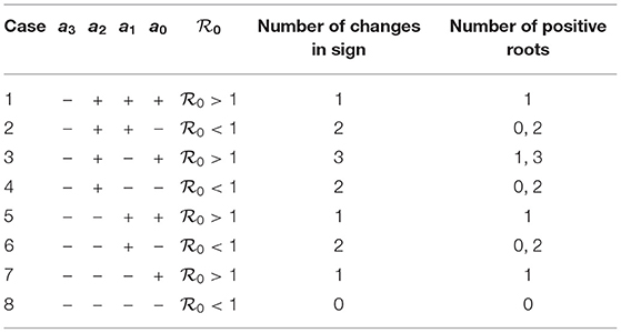
Table 1. Number of positive roots of Equation (12).

Theorem 2. The system (5-7)

1. has a unique steady state solution if ${{R}}_0>1$ and whenever cases 1, 5, and 7 are satisfied;

2. can have more than one steady state solution if ${{R}}_0>1$ and case 3 is satisfied;

3. can have two steady state solutions if ${{R}}_0<1$ and cases 2, 4, and 6 are satisfied.

The results of Table 1 can be described qualitatively using bifurcation diagrams. It can be seen from the table that for ${{R}}_0<1$ [cases (2,4,6,8)] there can be either two solutions or no solution. For ${{R}}_0>1$ there can be only one solution. The possibility of three solutions (case 3) can be ruled out since it can be shown that the cubic equation (Equation 12) for case 3 can not predict three positive solutions. Therefore, only two expected behavior can be found as far as the bifurcation diagram $({{R}}_0-i)$ is concerned. Figure 1A shows the case of two endemic equilibria for ${{R}}_0<1$ and one endemic equilibrium for ${{R}}_0>1$. Figure 1B shows, on the other hand, the case of the existence for ${{R}}_0<1$ of only the disease-free equilibrium (no endemic solution) and one endemic equilibrium for ${{R}}_0>1$.

FIGURE 1

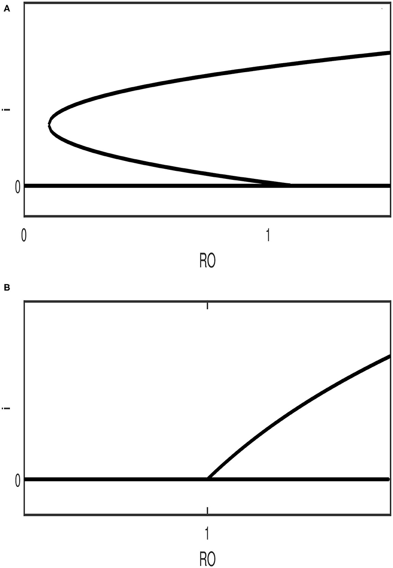
Figure 1. Qualitative diagrams showing the two possible bifurcation behavior expected in the model. (A) backward bifurcation; (B) forward bifurcation (The stability nature of the branches is ignored).

The steady state multiplicity for ${{R}}_0<1$ (Figure 1A) indicates the possible existence of a backward bifurcation where a stable endemic equilibrium coexists with the disease-free solution.

Before proceeding to the stability analysis, another useful relation can be obtained for the case of ${{R}}_0<1$. The analysis of the coefficients a_i(i = 0, 3) (Equation 12) shows that the following inequalities are always satisfied:

$\begin{array}{l}{\beta }_1-{\beta }_2-{\gamma }_1-\mu <{\beta }_1-{\beta }_2-{\gamma }_0-\mu <{\beta }_1-{\gamma }_0-\mu \\ \text{ since }{\gamma }_1>{\gamma }_0\text{and }{\beta }_2>0.& (14)\end{array}$

Therefore, if the last term in Equation (14) is negative i.e., β₁ ≤ μ + γ₀ the other terms of Equation (14) are also negative and therefore a₃ and a₂ are always negative which means that no positive solution can exist under this condition.

5. Stability of the Disease-Free Equilibrium

In this section we study the stability of the disease-free equilibrium point E₀.

Theorem 3. For the nonlinear dynamical system (Equations 5–6)

 1. if ${{R}}_0<1$ then E₀ is an attracting node;

 2. if ${{R}}_0>1$ then E₀ is a saddle;

 3. if ${{R}}_0=1$ then E₀ is non-hyperbolic, and

(a) if $a_{11}=\left(\frac{{\beta }_2}{m}+\frac{{\gamma }_1-{\gamma }_0}{b}-\frac{{{\beta }_1}^2}{\mu }\right)\ne 0$, E₀ is a saddle-node.

(b) if a₁₁ = 0 and $a_{22}=\left(\frac{{\beta }_2{\gamma }_1}{\mu m}+\frac{{\beta }_1({\gamma }_1-{\gamma }_0)}{\mu b}-\frac{{{\beta }_1}^2{\gamma }_1}{{\mu }^2}\right)<0$ then E₀ is an attracting node.

Proof: The Jacobian matrix J(E₀) of the system (Equations 5–6) at E₀ is given by

$\begin{array}{ll}J(E_0)=\left[\begin{array}{cc}-\mu & -{\beta }_1\\ 0& {\beta }_1-{\gamma }_1-\mu \end{array}\right].& (15)\end{array}$

The eigenvalues of the matrix Equation (15) are ${\lambda }_1={\beta }_1-{\gamma }_1-\mu =({\gamma }_1+\mu )({{R}}_0-1)$ and λ₂ = −μ. Therefore, we can see that if R₀ < 1 then E₀ is an attracting node and is a saddle if ${{R}}_0>1$.

In the case of ${{R}}_0=1$ the first eigenvalue is zero (λ₁ = 0) and E₀ is a non-hyperbolic point. In order to examine the nature of E₀ we make use of the center manifold theory. We first transform the model (Equations 5–6) into the origin. Let u = s−1 and v = i then we have:

$\begin{array}{ll}\frac{du}{dt}=\mu -{\beta }_1(u+1)v-\frac{{\beta }_2(u+1)v^2}{m+v}-\mu (u+1)& (16)\end{array}$

$\begin{array}{ll}\frac{dv}{dt}={\beta }_1(u+1)v+\frac{{\beta }_2(u+1)v^2}{m+v}-\left({\gamma }_0+\frac{({\gamma }_1-{\gamma }_0)b}{v+b}+\mu \right)v.& (17)\end{array}$

Expanding the system (Equations 16–17) in a second order Taylor series around (u, v) = (0, 0) yields

$\begin{array}{ll}\frac{du}{dt}=-\mu u-{\beta }_{1}v-{\beta }_{1}uv-\frac{{\beta }_2{v}^2}{m}& (18)\end{array}$

$\begin{array}{ll}\frac{dv}{dt}=({\beta }_1-{\gamma }_1-\mu )v+{\beta }_{1}uv+\left(\frac{{\beta }_2}{m}+\frac{{\gamma }_1-{\gamma }_0}{b}\right)v^2.& (19)\end{array}$

When ${{R}}_0=1$ then β₁ − γ₁ − μ = 0 and the system (Equations 18–19) becomes:

$\begin{array}{ll}\frac{du}{dt}=-\mu u-{\beta }_{1}v-{\beta }_{1}uv-\frac{{\beta }_2{v}^2}{m}& (20)\end{array}$

$\begin{array}{ll}\frac{dv}{dt}={\beta }_{1}uv+\left(\frac{{\beta }_2}{m}+\frac{{\gamma }_1-{\gamma }_0}{b}\right)v^2.& (21)\end{array}$

The Jacobian matrix of the system is

$\begin{array}{ll}J=\left[\begin{array}{cc}-\mu & -{\beta }_1\\ 0& 0\end{array}\right]& (22)\end{array}$

with eigenvalues

$\begin{array}{ll}\left[\begin{array}{c}0\\ -\mu \end{array}\right].& (23)\end{array}$

We can therefore rewrite the system (Equations 20–21) as follows:

$\begin{array}{ll}\frac{dx}{dt}=a_{11}{x}^2+{\beta }_{1}xy,& (24)\end{array}$

$\begin{array}{ll}\frac{dy}{dt}=-\mu y+a_{22}{x}^2+a_{33}xy& (25)\end{array}$

with

$\begin{array}{l}{a}_{11}=\left(\frac{{\beta }_2}{m}+\frac{{\gamma }_1-{\gamma }_0}{b}-\frac{{{\beta }_1}^2}{\mu }\right),\\ a_{22}=\left(\frac{{\beta }_2{\gamma }_1}{\mu m}+\frac{{\beta }_1({\gamma }_1-{\gamma }_0)}{\mu b}-\frac{{{\beta }_1}^2{\gamma }_1}{{\mu }^2}\right),\\ a_{33}=\frac{{\gamma }_1{\beta }_1}{\mu }.\end{array}$

If a₁₁ ≠ 0 i.e., $b\ne \frac{({\beta }_1^{2}m-{\beta }_2\mu )}{\mu m({\gamma }_1-{\gamma }_0)}$ then it can be seen from (Equations 24–25) that E₀ is a saddle-node.

If a₁₁ = 0 i.e., $b=\frac{({\beta }_1^{2}m-{\beta }_2\mu )}{\mu m({\gamma }_1-{\gamma }_0)}$ then we restrict the system (Equations 24–25) to the center manifold parameterized by $y=h(x)=c_1{x}^2+c_2{x}^3$ where c₁ and c₂ are parameters that need to be determined. The dynamics on the center manifold can be shown to be described by:

$\begin{array}{l}{x}^{\prime }=\frac{{\beta }_1{a}_{22}}{\mu }{x}^3+\text{higher orders}\\ y^{\prime }=-\mu y+\text{higher orders}.\end{array}$

Therefore, E₀ is stable if a₁₁ = 0 and a₂₂ < 0. Substituting the condition a₁₁ = 0 into a₂₂ yields

$\begin{array}{ll}{a}_{22}={\beta }_1^2-\frac{{\beta }_2\mu }{m}.& (26)\end{array}$

The condition a₂₂ < 0 requires that

$\begin{array}{ll}{\beta }_1^2<\frac{{\beta }_2\mu }{m},& (27)\end{array}$

otherwise point E₀ is unstable.

6. Bifurcation

6.1. Backward Bifurcation

In this section we set up the conditions under which the model exhibits a backward bifurcation.

Theorem 4. The system (Equations 5–6) exhibits a backward bifurcation whenever $b<b_{cr}=\frac{{\gamma }_1-{\gamma }_0}{\frac{{({\gamma }_1+\mu )}^2}{\mu }-\frac{{\beta }_2}{m}}$ and no backward bifurcation otherwise.

Proof: We examine the existence of a backward bifurcation using the methodology described in [26]. First, we make the transformation of variables as follows: x₁ = s, x₂ = i. The model (Equations 5–6) is rewritten as follows:

$\begin{array}{ll}\frac{d{x}_1}{dt}=f_1=\mu -{\beta }_1{x}_1{x}_2-\frac{{\beta }_2{x}_1{x_2}^2}{(m+x_2)}-\mu x_1& (28)\end{array}$

$\begin{array}{ll}\frac{d{x}_2}{dt}=f_2={\beta }_1{x}_1{x}_2+\frac{{\beta }_2{x}_1{x_2}^2}{(m+x_2)}-(\gamma +\mu )x_2.& (29)\end{array}$

We assume the bifurcation parameter to be β₁. The condition ${{R}}_0=1$ corresponds to ${\beta }_1={\gamma }_1+\mu :={\beta }_1^{*}$. For ${\beta }_1={\beta }_1^{*}$, the Jacobian matrix of the system (Equations 28–29) at the disease-free equilibrium E₀ = (1, 0) is given by

$\begin{array}{ll}J=\left[\begin{array}{cc}-\mu & -{\beta }_1\\ 0& {\beta }_1-{\beta }_1^{*}\end{array}\right].& (30)\end{array}$

The right eigenvector of this matrix at the zero eigenvalue is $W={(w_1,w_2)}^T=(-\frac{{\beta }_1^{*}}{\mu },1).$ Similarly, the left eigenvector is given by V = (v₁, v₂) = (0, 1). The stability parameters (a) and (b) that determine the conditions for the existence of a backward bifurcation can be found by the methodology explained in [26]. The coefficient (a) is given by:

$\begin{array}{ll}\text{a}={\displaystyle \sum _{k,i,j=1}^2}{v}_k{w}_i{w}_j\frac{{\partial }^2{f}_k}{\partial x_i\partial x_j},& (31)\end{array}$

which is reduced (since v₁ = 0 and v₂ = 1) to

$\begin{array}{ll}\text{a}=w_1{w}_1\frac{{\partial }^2{f}_2}{\partial x_1^2}+2w_1{w}_2\frac{{\partial }^2{f}_2}{\partial x_1\partial x_2}+w_2{w}_2\frac{{\partial }^2{f}_2}{\partial x_2^2}.& (32)\end{array}$

The different derivatives evaluated at E₀ are given by

$\begin{array}{l}\frac{{\partial }^2{f}_2}{\partial x_1^2}=0\\ \frac{{\partial }^2{f}_2}{\partial x_1\partial x_2}={\beta }_1^{*}\\ \frac{{\partial }^2{f}_2}{\partial x_2^2}=\frac{2({\gamma }_1-{\gamma }_0)}{b}+\frac{2{\beta }_2}{m}.\end{array}$

Substituting yields

$\begin{array}{ll}\text{a}=\frac{2({\gamma }_1-{\gamma }_0)}{b}+\frac{2{\beta }_2}{m}-\frac{2{\beta }_1(\mu +{\gamma }_1)}{\mu }& (33)\end{array}$

On the other hand, the bifurcation parameter b is given by

$\begin{array}{ll}\text{b}={\displaystyle \sum _{k,i=1}^2}{v}_k{w}_i\frac{{\partial }^2{f}_k}{\partial x_i\partial {\beta }_1}& (34)\end{array}$

which is reduced to

$\begin{array}{ll}\text{b}=w_2\frac{{\partial }^2{f}_2}{\partial x_1\partial {\beta }_1}+w_2\frac{{\partial }^2{f}_2}{\partial x_2\partial {\beta }_1},& (35)\end{array}$

and can be shown to be equal to 1.

We conclude therefore that since b = 1 is always positive then the system exhibits a backward bifurcation when a > 0. The condition a > 0 is equivalent to

$\begin{array}{ll}\frac{{\gamma }_1-{\gamma }_0}{b}>\frac{{({\gamma }_1+\mu )}^2}{\mu }-\frac{{\beta }_2}{m}& (36)\end{array}$

It can be seen that in the absence of media effects i.e., β₂ = 0 the condition Equation (36) can be satisfied for some values of hospital-bed to population ratio (b). However, in the presence of media effects β₂ ≠ 0 and if the right hand side of the inequality is negative i.e.,

$\begin{array}{ll}\frac{{\beta }_2}{m}>\frac{{({\gamma }_1+\mu )}^2}{\mu },& (37)\end{array}$

then the inequality (36) is always satisfied for any values of b. This means that media awareness also plays a critical role in the occurrence/absence of a backward bifurcation. If, on other hand, the inequality (37) is not satisfied then a backward bifurcation occurs when

$\begin{array}{ll}b<\frac{{\gamma }_1-{\gamma }_0}{\frac{{({\gamma }_1+\mu )}^2}{\mu }-\frac{{\beta }_2}{m}}& (38)\end{array}$

6.2. Hopf Bifurcation

In this section we study the Hopf bifurcation of Equations (5−−6). The Jacobian matrix is

$\begin{array}{ll}J(s,i)=\left[\begin{array}{cc}{J}_{11}& J_{12}\\ J_{21}& J_{22}\end{array}\right],& (39)\end{array}$

where

$\begin{array}{l}{J}_{11}=-[{\beta }_{1}i+\frac{{\beta }_2{i}^2}{m+i}+\mu ],\\ J_{21}=-[{\beta }_{1}s+\frac{{\beta }_{2}si(2m+i)}{{(m+i)}^2}],\\ J_{21}={\beta }_{1}i+\frac{{\beta }_2{i}^2}{m+i},\\ J_{22}={\beta }_{1}s+2\frac{{\beta }_{2}si}{m+i}-\frac{{\beta }_{2}s{i}^2}{{(m+i)}^2}+\frac{({\gamma }_1-{\gamma }_0)bi}{{(i+b)}^2}-{\gamma }_0\\ -\frac{({\gamma }_1-{\gamma }_0)b}{i+b}-\mu .& (40)\end{array}$

We use the fact that along the steady state solution we have

$\begin{array}{r}{\beta }_{1}i+\frac{{\beta }_2{i}^2}{m+i}+\mu =\frac{\mu }{s},\\ {\beta }_{1}s+\frac{{\beta }_{2}si}{m+i}-{\gamma }_0-\frac{({\gamma }_1-{\gamma }_0)b}{\text{I}+b}-\mu =0.\end{array}$

Thus, we have

$\begin{array}{l}{J}_{22}=\frac{{\beta }_{2}sim}{{(m+i)}^2}-\frac{({\gamma }_0-{\gamma }_1)bi}{{(i+b)}^2},\\ \text{Trace}\left(\text{J}\right)=J_{11}+J_{22}=-\left(\beta 1i+\frac{{\beta }_2{i}^2}{m+i}+\mu \right)+\frac{{\beta }_{2}sim}{{(m+i)}^2}\\ -\frac{({\gamma }_0-{\gamma }_1)bi}{{(i+b)}^2}.& (41)\end{array}$

We can write this equation as follows:

$\begin{array}{ll}\text{Trace(J)}=-\frac{\Phi (i)}{{(m+i)}^2{(i+b)}^2\mu }& (42)\end{array}$

where

$\begin{array}{ll}\Phi (i)=B_5{i}^5+B_4{i}^4+B_3{i}^3+B_2{i}^2+B_{1}i+B_0& (43)\end{array}$

with

$\begin{array}{l}{B}_5=\mu ({\beta }_1+{\beta }_2),\\ B_4={\mu }^2+2({\beta }_1+{\beta }_2)(b+m)\mu +{\beta }_2{\gamma }_{0}m,\\ B_3=\mu ({\beta }_1+{\beta }_2)b^2+{\beta }_1\mu m^2+m\mu (2\mu -{\beta }_2)\\ +((4{\beta }_1\mu +{\gamma }_0{\beta }_2+{\gamma }_1{\beta }_2+4{\beta }_2\mu )m\\ +\mu ({\gamma }_0-{\gamma }_1+2\mu ))b,\\ B_2={m_1}^2{\mu }^2+((2{\beta }_1\mu +{\gamma }_1{\beta }_2+2{\beta }_2\mu )m+{\mu }^2)b^2\\ +(2{\beta }_1\mu m^2+2\mu ({\gamma }_0-{\gamma }_1+2\mu -{\beta }_2)m)b\\ B_1=({\beta }_1\mu m^2+\mu (2\mu -{\beta }_2)m)b^2+\mu ({\gamma }_0-{\gamma }_1+2\mu )m^2{b}_1\\ B_0=b^2{m}^2{\mu }^2.& (44)\end{array}$

The coefficients of Equation (44) are always positive when the following condition holds

$\begin{array}{ll}{\beta }_2\le {\gamma }_0-{\gamma }_1+2\mu & (45)\end{array}$

Simple analysis shows that the maximum value of γ₁ when the right side of the condition (45) is positive satisfies

$\begin{array}{ll}{\gamma }_{1,max}\le 2\mu +{\gamma }_0.& (46)\end{array}$

The other condition of Hopf point Det(J) > 0 can also be readily derived. However, both Hopf conditions are not easily amenable to analytical manipulations and therefore numerical simulations are used to illustrate the Hopf-induced dynamics of the model.

7. Numerical Simulations

In order to carry out numerical simulations we needed first to choose carefully the values of model parameters that reflect the disease parameters in Saudi Arabia, a country that has recorded more than 362,000 cases as on December 25, 2020 [27]. Only two model parameters were assumed constant: the natural death rate μ which is 4.21 × 10⁻⁵ [28] and the hospital-bed to population ratio which is 22 per 10,000 [29]. The rest of model parameters (m, β₁, β₂, γ₀, γ₁) were fitted to COVID-19 data in the country. The fitting was carried out with the help of the optimization function (fmincon) of MATLAB. The COVID-19 data used for fitting consist of infected cases and removed (recovered and deceased) cases. The data was collected for a period of 90 days starting from March 2 (the day of the detection of the first COVID-19 case in the country) until June 2. The data is publicly accessible via the COVID-19 dashboard of the Saudi Ministry of Health [27]. The reason we restricted the data to this period is to be able to compare the obtained reproduction number with similar results available in the literature [30, 31].

Figure 2 shows the fitting results. Both the infected cases (Figure 2A) and removed cases (Figure 2B) show a reasonable quality of fit. Since the optimization task led to local optima, we were guided by the results reported in [22, 30, 31] in selecting initial conditions and bounds on the fitted model parameters. The optimum values of model parameters are shown in Table 2.

FIGURE 2

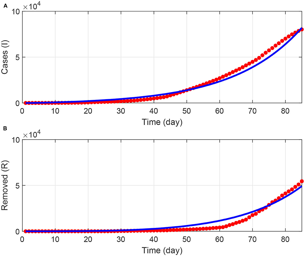
Figure 2. (A,B) Results of fitting the model to COVID-19 data in Saudi Arabia for a period of 90 days starting from March 2, 2020. Blue solid line (model predictions); red points (actual data).

TABLE 2

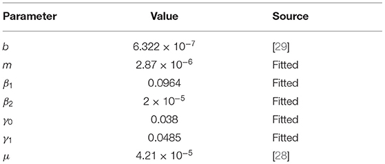
Table 2. Model parameters.

For bifurcation studies the basic reproduction number ${{R}}_0$ was taken to be the main bifurcation parameter so the transmission rate β₁ can be calculated by ${\beta }_1={{R}}_0({\gamma }_1+\mu )$ (Equation 13). The bifurcation diagrams were obtained using the continuation software AUTO [32]. Using the obtained values of model parameters, the condition (Equation 38) for a backward bifurcation to occur can be shown to be b < 2.01 × 10⁻⁴. Figure 3 shows an example of bifurcation diagrams in the (${{R}}_0-i$) plane for b = 6.322 × 10⁻⁷. This is the actual value of the dimensionless hospital-bed to population ratio, and can be seen to be much smaller than the aforementioned critical value. Saddle-node bifurcation can be seen to occur in this case. A static limit point LP appears at ${{R}}_0=0.803$. The diagram is also characterized by the presence of a Hopf point occurring at ${{R}}_0=0.896$. An unstable limit cycle can be seen to emerge from the Hopf point and disappears from homoclinic bifurcation. Here we have a situation where the disease-free equilibrium coexists with the endemic equilibrium for the range of basic reproduction number extending from HB $({{R}}_0=0.896)$ to $({{R}}_0=1)$.

FIGURE 3

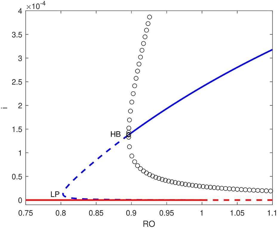
Figure 3. Bifurcation diagram for b = 6.322 × 10⁻⁷ showing a backward bifurcation. solid line (stable branch); dashed line (unstable branch); circles (unstable periodic branches); LP (static limit point); HB (Hopf point); blue line (endemic equilibrium); red line (disease free equilibrium).

Figures 4A,B show numerical simulations for the Hopf point and the limit cycle. Figure 4A shows the birth of a limit cycle close to the Hopf point while Figure 4B shows an example of time trace of an unstable limit cycle at $({{R}}_0=0.899)$. The oscillations grow in magnitude until they terminate as they collide with the static branch (S = 1).

FIGURE 4

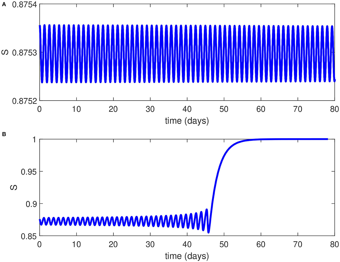
Figure 4. (A) Time trace close to the Hopf point ${{R}}_0=0.896$ of Figure 3. (B) Time trace for ${{R}}_0=0.899$ of Figure 3 showing unstable oscillations growing in magnitude until they collide with the static branch.

From an epidemiological perspective, the existence of a Hopf point in the model and the nature of the Hopf bifurcation (subcritical) has two effects on the dynamics of the disease transmission: (1) The endemic equilibrium coexists now with the disease-free solution for values of ${{R}}_0$ ranging from the Hopf point to ${{R}}_0=1$. This means that even if the basic reproduction number is reduced below unity, it is still possible for the pandemic to persist unless the reproduction number is reduced below the point associated with the Hopf point (HB, ${{R}}_0=0.896$). (2) The existence of a subcritical Hopf bifurcation (as opposed to supercritical when a stable limit cycle surrounds an unstable equilibrium point) means that the pandemic cannot have a stable periodic behavior and this is consistent with the current situation in the country which showed a steady decline in the disease active cases. Even if initial conditions (S, I) would fall close to the limit cycle, the resulting unstable oscillations would increase in magnitude but they will ultimately collapse and lead to the disease suppression (Figure 4B).

Figure 5 shows, on the other hand, the bifurcation diagram for b = 2.5 × 10⁻⁴, a value just larger than the aforementioned critical point. The backward bifurcation disappears and we have the occurrence of a forward bifurcation where the endemic equilibrium is the only stable point. A forward bifurcation is of course the outcome to aim for in a pandemic since if the basic reproduction number is reduced to a value below unity, then the disease outbreak is suppressed. Figures 3, 5 therefore showed the important role the number of hospital beds plays in the control of the pandemic. However from a practical point of view, the current hospital-bed to population ratio (22 per 10,000 people) is much smaller than the critical value. This means that a forward bifurcation is unlikely.

FIGURE 5

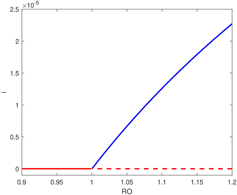
Figure 5. Bifurcation diagram for b = 2.5 × 10⁻⁴ showing forward bifurcation; solid line (stable branch); dashed line (unstable branch); blue line (endemic equilibrium); red line (disease free equilibrium).

Next, we examine the effects of variations in model parameters on the occurrence of the backward bifurcation. This can be suitably done by showing the location of the Hopf point when these parameters are varied, as shown in Figures 6A–E obtained also using AUTO. These figures are quite useful since they illustrate the range of the backward bifurcation, that is the range in term of ${{R}}_0$ of the stable coexistence of the endemic equilibrium with the disease-free equilibrium. This sensitivity analysis is also necessary given the unavoidable degree of uncertainty in the fitted values of model parameters.

FIGURE 6

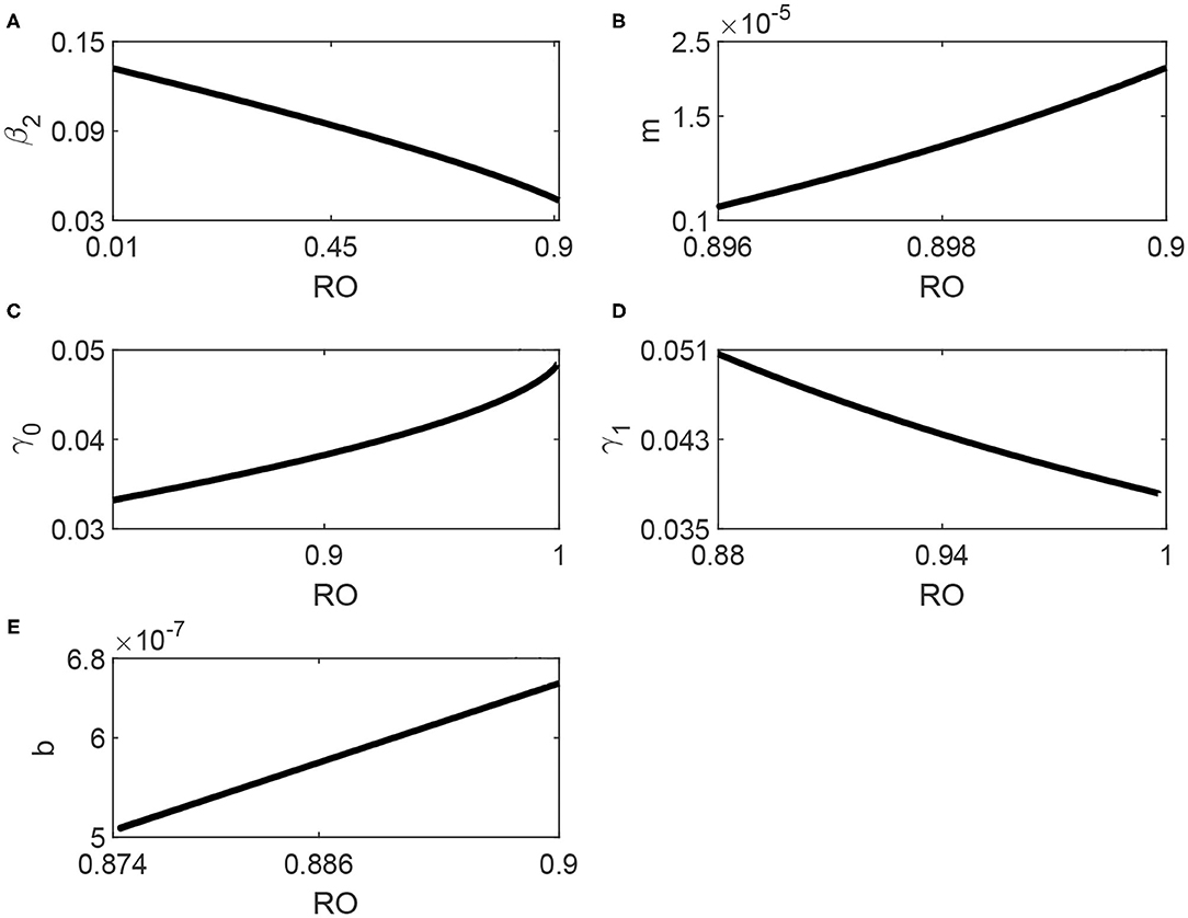
Figure 6. (A–E) Locus of the Hopf point of Figure 3 in terms of the model parameters.

We start with the effects of media shown in Figures 6A,B. The media effects are represented by two parameters: the awareness rate β₂ and the half-saturation constant m. It can be seen from Figure 6A that the range of backward bifurcation decreased in term of ${{R}}_0$ since the Hopf point moves to large values. The effect of m (Figure 6B) shows that as m increases the Hopf point moves to larger values of ${{R}}_0$ which means again a smaller range of coexistence with the disease-free equilibrium. We can therefore conclude that the media also have an important role in attenuating the backward bifurcation.

Figure 6C shows, on the other hand, the effects of the minimum removal rate γ₀. It can be seen that larger values of γ₀ decrease the range of the coexistence since the Hopf point moves to larger values and closer to 1. The effect of the maximum removal rate γ₁ is shown in Figure 6D. Unlike γ₀, it can be seen that as γ₁ decreases, the Hopf point moves to larger values of ${{R}}_0$. While it is true that the values of γ₀ and γ₁ depend on the inherent properties of the virus causing the COVID-19 disease, they also depend on health care and basic clinical resources [14]. Their role is therefore important in attenuating the backward bifurcation. Finally, Figure 6E shows that as the hospital-bed to population ratio b increases, the location of the Hopf point moves to larger values of ${{R}}_0$. This confirms the already obtained results that the backward bifurcation is reduced with the increase in available hospital beds.

8. Conclusions

The paper examined the dynamics of a SIR model applied to COVID-19 disease with two modifications: (1) the removal rate was assumed to be nonlinear and function of both the number of infectious individuals and hospital-bed to population ratio; (2) the model included public awareness due to media. The model was validated using COVID-19 data pertinent to Saudi Arabia. The model was shown to exhibit backward and Hopf bifurcations. The Hopf point is subcritical and unstable limit cycles terminate homoclinically. Therefore no stable periodic behavior occurred in the model for the chosen set of parameters. The main behavior observed in the model is a static coexistence of the disease-free equilibrium with the endemic point for a range of the basic reproduction number extending from the Hopf point to ${{R}}_0=1$. The analysis also showed the important role played by health care resources in term of hospital-bed to populations ratio as well as the minimum and maximum removal rates. In fact with the country's current health resources, a backward bifurcation is the most likely outcome and can be attenuated by the increase in the media awareness.

Data Availability Statement

The original contributions presented in the study are included in the article/supplementary material, further inquiries can be directed to the corresponding author/s.

Author Contributions

All authors listed have made a substantial, direct and intellectual contribution to the work, and approved it for publication.

Conflict of Interest

The authors declare that the research was conducted in the absence of any commercial or financial relationships that could be construed as a potential conflict of interest.

Acknowledgments

The authors extend their appreciation to the Deanship of Scientific Research at King Saud University for funding this work through research group no (RG-1441-188).

References

1. Chen TM, Rui J, Wang QP, Zhao ZY, Cui JA, Yin L. A mathematical model for simulation the phase-based transmissibility of novel coronavirus. Infect Dis Pov. (2020) 9:24. doi: 10.1186/s40249-020-00640-3

CrossRef Full Text | Google Scholar

2. Bentout S, Chekroun A, Kuniya T. Parameter estimation and prediction for corona virus disease outbreak 2019 (COVID-19) in Algeria. AIMS Public Health. (2020) 7:306–18. doi: 10.3934/publichealth.2020026

PubMed Abstract | CrossRef Full Text | Google Scholar

3. Belgaid Y, Helal M, Venturino E. Analysis of a model for Corona virus spread. Mathematics. (2020) 8:820. doi: 10.3390/math8050820

CrossRef Full Text | Google Scholar

4. Mishra AM, Purohit SD, Owolabi KM, Sharma YD. A nonlinear epidemiological model considering asymptotic and quarantine classes for SARS CoV-2 virus. Chaos Soliton Fract. (2020) 138:109953. doi: 10.1016/j.chaos.2020.109953

PubMed Abstract | CrossRef Full Text | Google Scholar

5. Kwuimy CAK, Nazari F, Jiao X, Rohani P, Nataraj C. Nonlinear dynamic analysis of an epidemiological model for COVID-19 including public behavior and government action. Nonlinear Dyn. (2020) 101:1545–59. doi: 10.1007/s11071-020-05815-z

PubMed Abstract | CrossRef Full Text | Google Scholar

6. Brauer F, Castillo-Chavez C. Mathematical Models in Population Biology and Epidemiology. New York, NY: Springer-Verlag (2001).

Google Scholar

7. Diekmann O, Heesterbeek JAP. Mathematical Epidemiology of Infectious Diseases: Model Building, Analysis and Interpretation. New York, NY: John Wiley & Sons Ltd. (2000).

Google Scholar

8. Hethcote HW. The mathematics of infectious disease. SIAM Rev. (2000) 42:599–653. doi: 10.1137/S0036144500371907

CrossRef Full Text | Google Scholar

9. Ruan S, Wang W. Dynamical behavior of an epidemic model with a nonlinear incidence rate. J Differ Equat. (2003) 188:135–63. doi: 10.1016/S0022-0396(02)00089-X

CrossRef Full Text | Google Scholar

10. Tang Y, Huang D, Ruan S, Zhang W. Coexistence of limit cycles and homoclinic loops in a SIRS model with a nonlinear incidence rate. SIAM J Appl Math. (2008) 69:621–39. doi: 10.1137/070700966

CrossRef Full Text | Google Scholar

11. Hu Z, Ma W, Ruan S. Analysis of SIR epidemic models with nonlinear incidence rate and treatment. Math Biosci. (2012) 238:12–20. doi: 10.1016/j.mbs.2012.03.010

PubMed Abstract | CrossRef Full Text | Google Scholar

12. Liu R, Wu J, Zhu H. Media/psychological impact on multiple outbreaks of emerging infectious diseases. Comput Math Methods Med. (2007) 8:612372. doi: 10.1080/17486700701425870

CrossRef Full Text

13. Wang W. Backward bifurcation of an epidemic model with treatment. Math Biosci. (2006) 201:58–71. doi: 10.1016/j.mbs.2005.12.022

PubMed Abstract | CrossRef Full Text | Google Scholar

14. Shan C, Zhu H. Bifurcations and complex dynamics of an SIR model with the impact of the number of hospital beds. J Differ Equat. (2014) 257:1662–88. doi: 10.1016/j.jde.2014.05.030

CrossRef Full Text | Google Scholar

15. Cui Q, Qiu Z, Liu W, Hu ZY. Complex dynamics of an SIR epidemic model with nonlinear saturate incidence and recovery rate. Entropy. (2017) 19:35. doi: 10.3390/e19070305

CrossRef Full Text | Google Scholar

16. Feng L, Jing S, Hu S, Wang DF, Huo HF. Modelling the effects of media coverage and quarantine on the COVID-19 infections in the UK. Math Biosci Eng. (2020) 17:3618–36. doi: 10.3934/mbe.2020204

PubMed Abstract | CrossRef Full Text | Google Scholar

17. Mohsen A, Al-Husseiny HF, Zhou X, Hattaf K. Global stability of COVID-19 model involving the quarantine strategy and media coverage effects. AIMS Public Health. (2020) 7:587–605. doi: 10.3934/publichealth.2020047

PubMed Abstract | CrossRef Full Text | Google Scholar

18. Marinov CT, Marinova RS. Dynamics of COVID-19 using inverse problem for coefficient identification in SIR epidemic models. Chaos Soliton Fract. (2020) 5:5100041. doi: 10.1016/j.csfx.2020.100041

CrossRef Full Text | Google Scholar

19. Comunian A, Gaburro R, Giudici M. Inversion of a SIR-based model: a critical analysis about the application to COVID-19 epidemic. Phys D. (2020) 413:132674. doi: 10.1016/j.physd.2020.132674

PubMed Abstract | CrossRef Full Text | Google Scholar

20. Giordano G, Blanchini F, Bruno R, Colaneri P, Di Filippo A, Di Matteo A, et al. Modelling the COVID-19 epidemic and implementation of population-wide interventions in Italy. Nat Med. (2020) 26:855–60. doi: 10.1038/s41591-020-0883-7

PubMed Abstract | CrossRef Full Text | Google Scholar

21. Keeling MJ, Dyson L, Guyver-Fletcher G, Holmes A, Semple MG, Tildesley MJ, et al. Fitting to the UK COVID-19 outbreak, short term forecasts and estimating the reproductive number. medRxiv. (2020). doi: 10.1101/2020.08.04.20163782

PubMed Abstract | CrossRef Full Text | Google Scholar

22. Alharbi Y, Alqahtani A, Albalawi O, Bakouri M. Epidemiological modeling of COVID-19 in Saudi Arabia: spread projection, awareness, and impact of treatment. Appl Sci. (2020) 10:5895. doi: 10.3390/app10175895

CrossRef Full Text | Google Scholar

23. Alrasheed H, Althnian A, Kurdi H, Al-Mgren H, Alharbi S. COVID-19 Spread in Saudi Arabia: modeling, simulation and analysis. Int J Environ Res Public Health. (2020) 17:7744. doi: 10.3390/ijerph17217744

PubMed Abstract | CrossRef Full Text | Google Scholar

24. Boaden R, Proudlove N, Wilson M. An exploratory study of bed management. J Manage Med. (1999) 13:234–50. doi: 10.1108/02689239910292945

CrossRef Full Text | Google Scholar

25. Van den Driessche P, Watmough J. Reproduction numbers and subthreshold endemic equilibria for compartmental models of disease transmission. Math Biosci. (2002) 180:29–48. doi: 10.1016/S0025-5564(02)00108-6

PubMed Abstract | CrossRef Full Text | Google Scholar

26. Castillo-Chavez C, Song B. Dynamical models of tuberculosis and their applications. Math Biosci Eng. (2004) 1:361–404. doi: 10.3934/mbe.2004.1.361

PubMed Abstract | CrossRef Full Text | Google Scholar

27. Saudi Arabia COVID-19 Dashboard. Available online at: https://covid19.moh.gov.sa/ (accessed November 2, 2020).

28. General Authority for Statistics. Available online at: https://www.stats.gov.sa/en/5305 (accessed November 2, 2020).

29. Saudi Ministry of Health. Available online at: https://www.moh.gov.sa/en/Pages/Default.aspx (accessed November 2, 2020).

Google Scholar

30. Aletreby W, Alharthy A, Faqihi F, Mady AF, Ramadan OE, Huwait BM, et al. Dynamics of SARS-CoV-2 outbreak in the Kingdom of Saudi Arabia: a predictive model, Saudi. Crit Care J. (2020) 4:79–83. doi: 10.4103/sccj.sccj_19_20

CrossRef Full Text | Google Scholar

31. Alshammari F. A Mathematical model to investigate the transmission of COVID-19 in the Kingdom of Saudi Arabia. Comput Math Method M. (2020) 2020:9136157. doi: 10.1155/2020/9136157

PubMed Abstract | CrossRef Full Text | Google Scholar

32. Doedel EJ, Kernevez JP. Auto: Software for Continuation and Bifurcation Problems in Ordinary Differential Equations. Pasadena, CA: Institute of Technology (1999).

Google Scholar