On Synthetic Instrument Response Functions of Time-Correlated Single-Photon Counting Based Fluorescence Lifetime Imaging Analysis

1 Introduction

Fluorescence lifetime imaging (FLIM) has become a versatile and powerful analytical tool for biomedical applications. Compared with fluorescence intensity imaging, FLIM is not only less susceptible to experimental artifacts in excitation/detection setups, optical paths, or fluorophore concentrations, but can also provide abundant cellular information [1–4]. FLIM offers a unique route for probing and visualizing intracellular physical parameters such as temperature, pH, O_2, and ion concentrations, and it can be promising for cancer diagnosis [5–9]. Furthermore, in combination with Föster resonance energy transfer (FRET) techniques, FLIM-FRET techniques are excellent tools for studying protein-protein interactions, cellular metabolisms, and conformational changes of proteins in living cells [10–12].

Measurements of fluorescence lifetimes can be carried out either directly in the time domain or indirectly in the frequency domain. In particular, time-correlated single-photon counting (TCSPC) has become the gold standard. It is prevailing among scientific communities for its abilities to offer better temporal resolution and signal-to-noize ratio (SNR) performances [13, 14]. A typical TCSPC FLIM system has an ultrafast pulse laser to excite the specimens and a single photon detector, either a photomultiplier tube (PMT) or a single-photon avalanche diode (SPAD), and a time-to-digital converter (TDC) to time-tag captured photons. By repeating this process, a temporal decay histogram can be built. The fluorescence decay measured in the time domain can be described by a sum of multiexponential decays [1]:

$f\left(t\right)={\displaystyle \sum _{i=1}^n{\alpha }_i{e}^{-t/{\tau }_i}}+\epsilon \left(t\ge 0\right)(1)$

where f(t) is the total fluorescence decay with n different exponential components. τ_i and α_i are the lifetime and corresponding fractional weight of the ith components, respectively. The sum of all fractional values, a1 + a2 +…, is normalized to 1 and ε represents the additional noise. However, since the duration of the excitation pulse and the temporal resolution of the TCSPC system cannot be ignored, the instrument response function (IRF) of the detection system should be considered. Therefore, the measured decay histogram y(t) is not the true fluorescence decay profile, f(t), of the specimens under inspection. Instead, it is f(t) convolved with the IRF, i(t).

$y\left(t\right)=f\left(t\right)\ast i\left(t\right)={\displaystyle \underset{\tau =0}{\overset{t}{\int }}f\left(\tau \right)}i\left(t-\tau \right)d\tau (2)$

The IRF is usually characterized by its full width at half maximum (FWHM), typically in several hundred picoseconds. It is a function of the uncertainties contributed from the laser excitation, the detector, and the TCSPC. To compensate the IRF and recover f(t), the IRF of the system needs to be measured in advance. And the fluorescence lifetimes of specimens are retrieved by the iterative deconvolution of a pre-defined single or multiple decay model with the measured IRF using nonlinear least-squares deconvolution (NLSD) methods. The result is compared with the recorded decay profile until the residual error is sufficiently small [14].

Ideally, the IRF of the system can be measured using a sample with an ultrashort lifetime [15]. In real FLIM systems, the samples can be dyes with a fluorescence lifetime about tens of picoseconds such as Erythrosine B, pinacyanol iodide, or Allura Red [16–19]. However, the sample lifetime is comparable to the temporal resolution of the TCSPC system. The measured IRF using these samples have a pronounced effect on the measurement of specimens like NAD(P)H, which has multiexponential decays with short lifetime components. In real experiments, the IRF signal is often hard to be detected because the quantum yield of fast decay fluorophores is low. Another drawback is that the spectral ranges of the dyes are limited. It is reported that the emission spectra of dyes with short fluorescence lifetimes only exist at the range larger than about 525 nm [20]. For example, the emission spectrum of pinacyanol iodide starts from 550 nm, and that of Allura Red is from 550 nm to 750 nm [16, 19]. No dye has been found with an emission spectrum covering all visible wavelengths. Therefore, it is difficult to find suitable dyes for every spectra window of interest. For a two-photon FLIM system, some other IRF measurement techniques based on Hyper-Rayleigh scattering (HRS) or second harmonic generation (SHG) have been proposed [21–23]. For example, the plasmon-enhanced gold luminescence can yield a wide-range ultrafast second-harmonic HRS signal, which can be used as a calibration sample for IRF measurements for a multiphoton FLIM system [22]. The second harmonic signal generated on the surface of urea crystals, potassium dihydrogen phosphate crystals or collagen fibers is also widely applied to measure the IRF [23]. However, there are still many restrictions that limit their performances. The HRS or SHG signals are easily corrupted by many artificial reflected or scattered signals in optical systems within the instrument.

Furthermore, the wavelengths of both HRS and SHG signals are only half of the excitation wavelength. Emission filters are required to ensure that signals are detected. For a multispectral FLIM system with multiple detectors, the situation becomes much more complex as the whole optical path should be rearranged to allow all detectors to detect signals effectively. Strictly speaking, the entire experimental setup should exactly keep the same with that for fluorescence lifetime measurements, or the measured IRF would be inaccurate. But this is difficult or impossible for many practical FLIM systems. Additionally, some detectors, especially for SPAD, have a wavelength-dependent temporal response known as the color effect [1]. In this case, the HRS or SHG signals cannot be used as the IRF should be measured within the same spectra with the fluorescence signals.

Measurements of IRF increase experimental complexity and burden. What is worse, for some clinic or in-vivo FLIM-based applications, the IRF cannot be measured. Hence, it is desirable to directly extract the IRF information from the recorded decay profiles without extra measurements. One method uses synthetic gaussian or single exponential decay function to approximate to IRF by adjusting its width and position to give the best fit to the fluorescence decay signal. Such a method shows good precision and a wide dynamic range that can resolve lifetimes close to the FWHM of the IRF. However, one critical drawback for TCSPC FLIM is time-consuming curve-fitting analysis. It becomes worse for the synthetic IRF due to an extra fitting and optimization to determine the synthetic function pixel by pixel. Another method uses an automatic synthetic IRF or differential synthetic IRF, widely adopted in commercial FLIM data analysis software, e.g., SPCImage (Becker and Hickl, Berlin, Germany). The calculation procedure of such a synthetic IRF can be divided into two steps: 1) the rising edge of the recorded decay profile is fitted with a suitable function R(t); 2) the synthetic IRF is then calculated as dR(t)/dt [24]. The synthetic IRF has been proved to yield precise fitting results in a deconvolution procedure. Nevertheless, the dynamic range of the synthetic IRF is limited. To obtain acceptable fitting results, the lifetimes of fluorescence signals should be several times longer than the FWHM of the IRF; otherwise, the analysis will be heavily biased. In this work, we proposed a new strategy to generate synthetic IRFs. This newly proposed synthetic IRF is directly extracted from the recorded summed decay histogram of all pixels, which has advantages: a broader dynamic range and higher accuracy. Bi-exponential fluorescence decay models were used in deconvolution procedures for more general FLIM-FRET applications. For better quantitively evaluations, simulated data was analyzed using a nonlinear least square deconvolution algorithm. Moreover, we also examined the fast deconvolution method’s deconvolution performance based on the Laguerre expansion with the proposed synthetic IRF. The real experimental FLIM-FRET data obtained from the two-photon FLIM system were further analyzed and compared using different automatic synthetic IRFs.

2 Theory and Method

For simplification, considering a single exponential decay f(t) = e^-t/τ. In order to evaluate i(t) from y(t), one can obtain the equation by performing both sides of Eq. 2 with the Laplace transform:

$I\left(s\right)=Y\left(s\right)/F\left(s\right)=sY\left(s\right)+\frac{1}{\tau }Y\left(s\right)(3)$

where Y(s), F(s), and I(s) are the Laplace transform pairs of y(t), f(t), and i(t), respectively. s is a complex-valued number. By performing the inverse Laplace transform on Eq. 3, The temporal IRF i(t) is then expressed as

$i\left(t\right)=\frac{dy\left(t\right)}{dt}+\frac{1}{\tau }y\left(t\right)(4)$

If the lifetime is large enough, the second item on the right side of Eq. 4 can be neglected, and the IRF can be directly estimated from the measured decay. This only holds for decay components with lifetimes much larger than the FWHM of IRF. However, if the lifetime is close to the FWHM of IRF, the estimated IRF is significantly shortened, which biases the calculated lifetimes toward longer values. As for multiexponential decays, since the overall decay is the linear combination of single exponential decays described in Eq. 1, the conclusion is also suitable for this situation. Thus, a compensation method needs to be proposed to extend the applied range of a synthetic IRF.

A series of noiseless decay curves with different lifetimes and their corresponding synthetic IRFs were analyzed to investigate the effect of a fast decay component on the synthetic IRF. A Gaussian function approximates the IRF with a typical FWHM, w = 300 ps, referred to as “the true IRF”, i₀(t). The measured decays were then generated by convolving single exponential decays with i₀(t) with 256 time-bins over a range of 10 ns. The synthetic IRF i_s(t) was obtained by calculating the measured decays' difference and setting the negative values to zero. Figure 1A shows the measured decays with three different lifetimes and their corresponding synthetic IRFs (i_s(t)). It is evident that as the lifetime τ increases, the difference between i_s(t) and i₀(t) diminishes as Eq. 4 suggests. On the contrary, when τ is approximate to w, for example, τ = 2w, the FWHM of i_s(t) is noticeably smaller than that of i₀(t). The results agree well with the above theoretical analysis. Another essential feature is that the fast decay components have more influence on the descending edge of the i_s(t), which accounts for the significant contribution to the decrement of the FWHM in i_s(t). For a smaller τ, the descending edge of i_s(t) has a steeper slope. On the contrary, the rising edge almost keeps unchanged as τ changes from 2w to 10w. To compensate for the influence of the fast decay component, one possible approach is to use the mirror symmetry of the rising edge to replace the descending edge. The new synthetic IRF can be then referred to as the mirror-symmetric synthetic IRF and denoted by i_m(t), which is calculated by

$i_m\left(t\right)=\frac{dy}{dt}u\left(t_0-t\right)+\frac{dy\left(t_0-t\right)}{dt}u\left(t-t_0\right)(5)$

where t₀ is the peak position of the i_s(t) and u(t) is the step function. Figure 1B shows the relative error of FWHM. The relative error is defined as | w_i -w|/w × 100 where w_i is the FWHM of i_s(t) or i_m(t). From Figure 1B, the error of i_s(t) shows an exponential increase when τ/w moves toward 1. In contrast, i_m(t) offers better performance. The error is much smaller than that of i_s(t) within the whole dynamic range. Even when the lifetime is the same as the FWHM of the IRF (τ = w), the error is still less than 10%. The precise evaluation of the IRF leads to better fitting results in the deconvolution procedure. Moreover, the dynamic range of the proposed IRF can be extended for faster decay components with a lifetime close to the FWHM of the IRF.

FIGURE 1

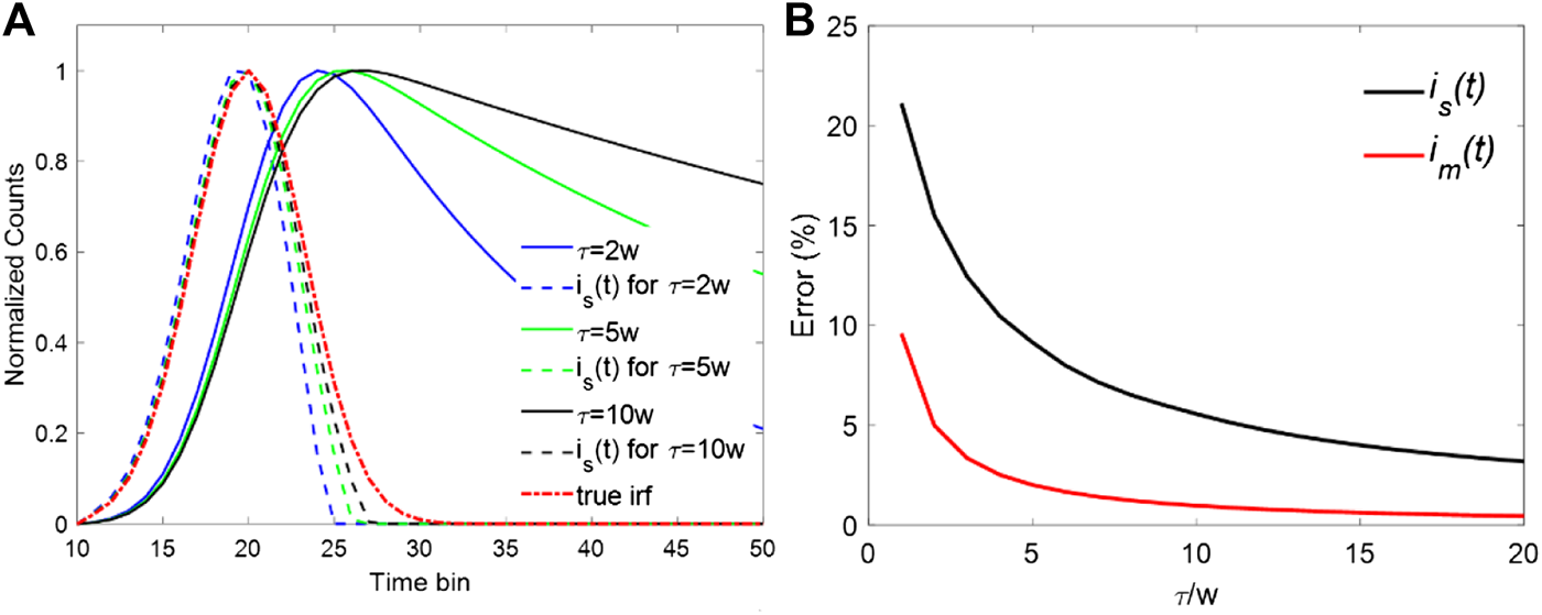
FIGURE 1. (A) Decay curves with different lifetimes and their synthetic IRFs. (B) Errors for i_s(t) and i_m(t) when τ/w is changing from 1 to 10.

3 Simulations on Fluorescence Lifetime Imaging Images

To compare the deconvolution performances of the two synthetic IRFs i_s(t) and i_m(t), both synthetic IRFs were tested with simulated TCSPC data. It is possible to calculate the bias accurately, and standard deviation since all simulated decays' parameters are already known. As shown in Eqs 1, 2, different synthetic IRFs are applied in the deconvolution procedure of TCSPC data with a various number of decay components. Here a bi-exponential decay with fast and slow decay components is considered. A bi-exponential decay model has broad applications and can be used to describe the quenched and unquenched states of fluorophores, the decays of endogenous fluorophores, and FRET donors, to name just a few [12]. A bi-exponential decay model is defined as

$f\left(t\right)=a{e}^{-t/{\tau }_1}+\left(1-a\right)e^{-t/{\tau }_2}(6)$

where τ₁ and τ₂ are the two different lifetimes and a is the proportion (0 < a < 1). The synthetic measured decays can then be generated by convolving f(t) and the pre-defined real IRF i_r(t)

$y\left(t_m\right)={\displaystyle \sum _{k=0}^m{i}_r\left(t_m-t_k\right)f\left(t_k\right)+{\epsilon }_m}m=\mathrm{1,2},\dots ,256(7)$

Here the observation window is T = 10 ns with 256 time-channels, and ε is the additive Poisson noise. i_r(t) has a Gaussian profile with w = 300 ps. In the simulations, a series of TCSPC FLIM images with 100 × 100 pixels were generated, and the total photon count per pixel within the observation window was assumed to be N_c. τ₂ is the longer lifetime and fixed at 2.8 ns, whereas τ₁ is a short lifetime varying from 0.2 to 1.0 ns. The proportion a ranges from 0.2 to 0.8 with a 0.2 step interval. Figures 2A,C show two examples of the simulated FLIM images' intensity map. The parameters in (a) and (b) are a = 0.4, τ₁ = 0.8 ns, τ₂ = 2.8 ns, N_c = 10,000 and a = 0.8, τ₁ = 0.4 ns, τ₂ = 2.8 ns, N_c = 5000, respectively. Due to the Poisson noise, the intensity of each pixel is slightly different and fluctuated around N_c. The corresponding phasor plots of (a) and (c) are shown in (b) and (d), respectively. In the phasor plots, the real and imaginary parts of the Fourier transform of the decay profile correspond to the horizontal and vertical coordinates, respectively. And the fluorescence decay detected in each pixel can be projected to a single point on a phasor plot [25–27]. In Figures 2B,D, the projected point of a single exponential decay is located on the semicircle, whereas that of a bi-exponential is located on the straight line between two different lifetimes. For a FLIM image with a relative lower N_c, the points are spread within a larger area, indicating that the noise has a pronounced effect on the decay profiles. The traditional method to estimate IRF is computationally complicated and inaccurate because the peak position varies due to the noise and jitter. Here, we propose a new approach to extract the IRF based on the measured FLIM images obtained by a single-channel scanning sensor: we estimated the IRF by summing all pixels' histograms together. Since the SNR of the Poisson noise is proportional to the photon count, the total decay can be regarded as a noise-free decay curve and is used for calculating the synthetic IRF. As shown in Figure 2E, the summed decay of all pixels, Y(t), and a decay in a pixel in Figure 2A are presented. Compared to a single decay curve, the noise has a negligible effect in Y(t). The two synthetic IRFs were then obtained from Y(t) and used for the deconvolution in each pixel.

FIGURE 2

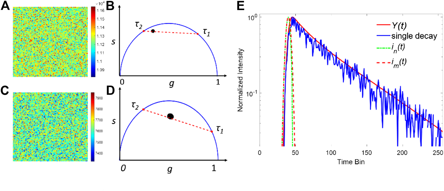
FIGURE 2. Simulated FILM images with a = 0.6, τ₁ = 0.8 ns, τ₂ = 2.8 ns, and N_c = 10,000 for (A) and a = 0.2, τ₁ = 0.4 ns, τ₂ = 2.8, and N_c = 5000 for (C). (B,D) are the corresponding phasor plots of (A,C). (E) Normalized intensity plots for Y(t) and the single decay in a pixel in (A). Generated synthetic IRFs using the total decay are depicted in dash lines.

Firstly, the nonlinear least-squares deconvolution (NLSD) based on the Levenberg-Marquardt algorithm was applied for recovering the parameters of the decays in Eq. 6. Figures 3A,C,E show the bias plots (Δa/a, Δτ₁/τ₁ and Δτ₂/τ₂) of the deconvolution fitting results using i_s(t) and i_m(t) with N_c = 10⁶. For better comparing i_s(t) and i_m(t), the photon counts were intendedly set to a high value so that the decay curves are less affected by noise. As a reference, a, τ₁and τ₂ were also calculated using the true IRF, i_r(t), for each pixel. The calculated a, τ₁ and τ₂ using i_s(t) have a larger bias within the whole dynamic range. When using i_s(t), Δa/a is generally larger than 10% and even reaches 100% when τ₁ is closed to 0.2 or 1 ns. The situation is worse for τ₁, where Δτ₁/τ₁ is around 100% for all cases, indicating that i_s(t) cannot be used for resolving τ₁. i_s(t) also failed to estimate τ₂ when τ₁ is closed to 1ns. In contrast, Δa/a, Δτ₁/τ₁ and Δτ₂/τ₂ are generally less than 1% using i_r(t). As for i_m(t), the biases are significantly reduced. The bias for all three parameters is lower than that of i_r(t). In particular, the bias of τ₂ for i_m(t) is the same as that of i_r(t).

FIGURE 3

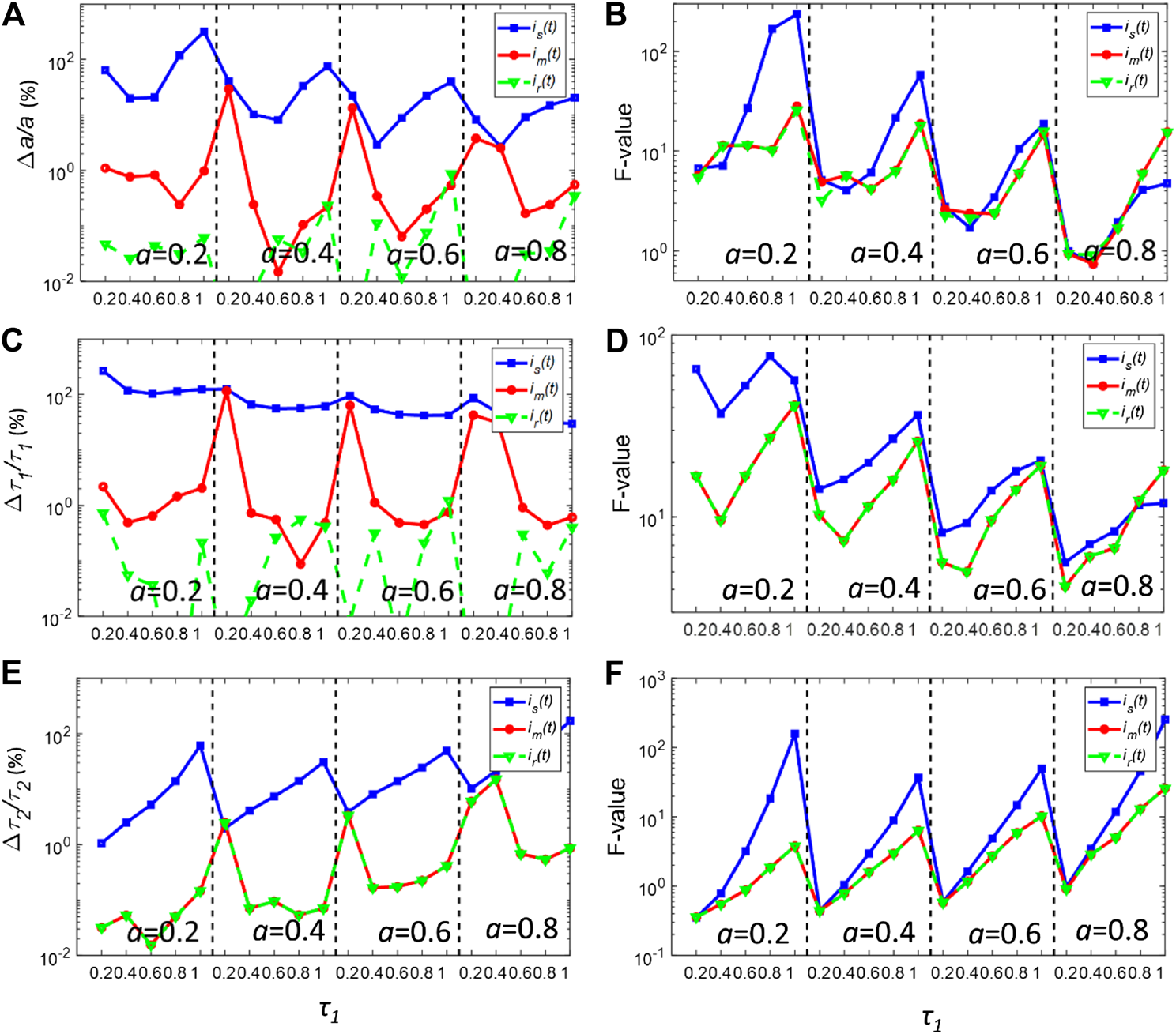
FIGURE 3. (A,C,E) normalized bias plots for a, τ₁ and τ₂ when N_c = 10⁶. The corresponding F-value plots are depicted in (B,D,F).

Figures 3B,D,E show the corresponding precision F-value = (σg/g)·N_c^0.5 (g = a, τ₁, or τ₂) plots for (a) (c) and (e), respectively, where σg is the standard deviation of g [28, 29]. For the ideal condition, F = 1. For most realistic FLIM analysis, F >> 1. The F-values for a, τ₁ and τ₂ using i_s(t) are in general larger than those using i_m(t) or i_r(t). Surprisingly, the F-values for i_m(t) and i_r(t) are nearly the same throughout the whole dynamic range. It also shows that using i_m(t) instead of i_s(t), the instability effect of the synthetic IRF on the deconvolution procedure can be eliminated.

The deconvolution performances of i_s(t) and i_m(t) under relatively low photon counts were also assessed. For many applications such as real-time FLIM imaging for investigating cell dynamics or high-throughput screening, the acquisition time is usually kept low, resulting in low photon counts in pixels. Figures 4A–F show the bias, and F-value plots for simulated fluorescence decays with N_c = 5000 in each pixel. In this case, the noise considerably distorts the decay curve. As shown in Figures 4A,C,E, all three IRFs yield worse bias performances compared with those shown in Figure 3. Also, the gaps between the bias plots for all three parameters decrease, showing that in low photon counts, the deconvolution procedure becomes insensitive to the differences between IRFs. Nevertheless, i_m(t) still shows better performances to resolve τ₂ when τ₁ is smaller than 1 ns. For determining τ₂, i_m(t) also yields similar performances with i_r(t). Moreover, i_m(t) has similar precision performances with i_r(t), showing smaller F-values for all variables compared with those of i_s(t). On the other hand, i_s(t) can yield an extremely large F-value for resolving τ₂. Therefore, it demonstrates that i_m(t) can provide a better estimation of the true IRF.

FIGURE 4

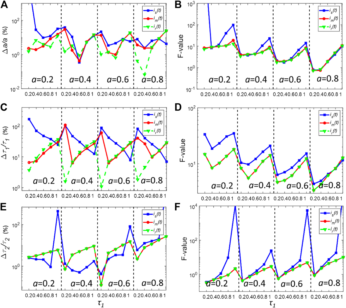
FIGURE 4. (A,C,E) Normalized bias plots for a, τ₁ and τ₂ when N_c = 5000. The corresponding F-value plots are depicted in (B,D,F).

Although NLSD fitting routines have been widely used for FLIM analysis, they still have intrinsic limitations. They are usually time-consuming and computationally intensive. Moreover, they are prone to overfitting problems when the fluorescence signal is heavily contaminated by noise. An alternative fast least-squares deconvolution based on Laguerre expansion (LSD-LE) was recently developed [30–34]. LSD-LE has been proven to be a robust and effective method showing much faster deconvolution speed than traditional methods. It also shows superior sensitivity in disease diagnoses. In brief, Eqs. 2, 6 can be rewritten in discrete forms；

$y\left(k\right)={\displaystyle \sum _{i=1}^{k}i\left(k-i\right)f\left(i\right)+\epsilon \left(k\right),}k=1,2,\dots ,N(8)$

$f\left(k\right)=a{e}^{-\left(k-1\right)t_s/{\tau }_1}+\left(1-a\right)e^{-\left(k-1\right)t_s/{\tau }_2}(9)$

where t_s is the time bin width. LSD-LE expands the fluorescence single f(t) onto an ordered set of orthonormal Laguerre basis functions b_l(k; α) as:

$\widehat{f}\left(k\right)={\displaystyle \sum _{l=0}^{L-1}{c}_l{b}_l\left(k;\alpha \right)}(10)$

where L is the Laguerre dimension and α (0<α < 1) is the scale parameter of LBF, and c_l is the lth expansion coefficient. The lth discrete LBF is defined as:

$b_l\left(k;\alpha \right)={\alpha }^{\left(k-1\right)}{\left(1-\alpha \right)}^{1/2}{\displaystyle \sum _{l=0}^{L-1}{\left(-1\right)}^i\left(\begin{array}{c}k\\ i\end{array}\right)\cdot \left(\begin{array}{c}l\\ i\end{array}\right)}{\alpha }^{1-i}{\left(1-a\right)}^i,l=0,1,\dots ,L-1(11)$

Under the Laguerre expansion, Eq. 9 becomes:

$y\left(k\right)={\displaystyle \sum _{i=0}^k{\displaystyle \sum _{l=0}^{L-1}{c}_{l}i\left(k-i\right)b_l\left(i;\alpha \right)+{\epsilon }_k}}(12)$

Equation 12 is the Laguerre expansion form of the fluorescence signal, which can be linearly parameterized by the expansion coefficient c_l. Also, the normalized sum of squared errors (NSSE) is defined as:

$NSSE={\left|\left|\widehat{f}-f\right|\right|}_2/{\left|\left|f\right|\right|}_2^2(13)$

To obtain the expansion coefficient c_l, the expansion of the fluorescence signal with LBFs becomes a fitting problem where NSSE reaches its minimal value. We would like to assess how i_s(t) behaves in Eq. 13. Therefore, the constrained LSD-LE is applied to recover the decay parameters using synthetic IRFs and the true IRF [30]. The LBF parameters were set as the optimized value as (α, L) = (0.92,16) [32]. The total photon counts in each pixel are N_c = 5000. The normalized bias and F-value plots are shown in Figures 5A–F. Not surprisingly, i_s(t) still has the worse performance (larger bias and F-value). It is unable to estimate τ₁ robustly. Meanwhile, it fails to recover τ₂ when τ₁ approaches 1 ns. i_m(t) has almost the same deconvolution results with the true IRF i_r(t) in terms of the bias and F-value. It further demonstrates that compensating the descending edge of synthetic IRF is an effective way to improve the precision and the applied lifetime range of the synthetic IRF.

FIGURE 5

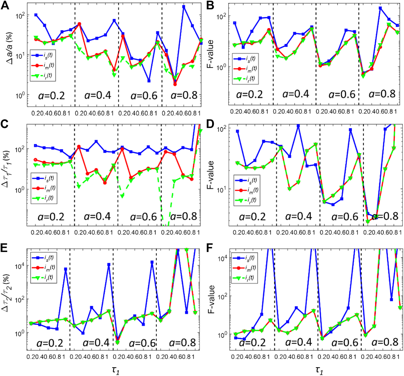
FIGURE 5. (A,C,E) Normalized bias plots for a, τ₁ and τ₂ when N_c = 5000 using LSD-LE method with (α, L) = (0.92,16). The corresponding F-value plots are depicted in (B,D,F).

4 Experimental Fluorescence Lifetime Imaging-Föster Resonance Energy Transfer Data Analysis

To evaluate the performances of the new automatic synthetic IRF in real experiments, FLIM-FRET imaging data of tSA201 cells transfected with eCFP-eYFP (enhanced green fluorescent protein and enhanced cyan fluorescence protein) pair were investigated. FLIM-FRET is a well-established technique for studying protein-protein interactions within a nanometer scale. FRET refers to the non-radiative energy transfer between an excited fluorescent molecule (the donor) and a non-excited different fluorescent molecule (the acceptor) when they are close, which leads to the shortening the donor lifetime. The eCFP-eYFP pair is the most widely used donor-acceptor pair in various in-vitro or in-vivo FRET applications. The lifetimes of the eCFP-eYFP pair with/without FRET are known priorly, thus serving as a reference to evaluate the FRET between interacting proteins. Here the FLIM-FRET technique was used to assess the proximity of interacting proteins.

A two-photon FLIM system including a confocal microscope (LSM 510, Carl Zeiss), a femtosecond Ti: sapphire laser modulated source (Chameleon, Coherent) with excitation wavelength 800 nm, and the TCSPC acquisition system (SPC-830, Becker and Hickl GmbH) was used to obtain IRF and FLIM data. The exciting laser source's duration is less than 200 fs, and the repetition rate is 80 MHz. The bin width of the TCSPC is 0.039 ns, and each measured histogram contains 256 time bins. Firstly, the IRF of the system was measured using the SHG signal from the urea ((NH₂)₂CO) microcrystal. A thin layer of urea crystal obtained from air-dry concentrated urea droplet was placed on a microscope slide and was covered by a coverslip. The emitted SHG signal was then collected by a photomultiplier (PCM-100, Becker & Hickl GmbH) after passing through a ×63 water-immersion objective lens (N.A. = 1.0) and a 650 nm short-pass filter. The emitted fluorescence signals from the cell samples were also collected using the same system except that a 535–590 nm bandpass filter was used.

The tSA201 cells were grown to 60% confluence on 13 mm glass coverslips located in 24 well plates. The cells were transfected with hP2Y₁₂-eCFP or co-transfected with hP2Y₁₂-eCFP and hP2Y₁-eYFP. After 48 h of transfection, the cells on the coverslips were washed once gently with PBS followed by fixation with ice-cold methanol for 10 min at room temperature. Then they were washed 3 times with PBS before they were mounted on to glass microscope slides with Mowiol. The microscope slides were then stored in the dark at room temperature overnight to allow the coverslips to dry, then held at 4°C for later use.

The analyzed results of tSA201cells with transfected co-transfected eYFP are shown in Figure 6. The eYFPs work as acceptors and their lifetimes increase when FRET occurs. Figure 6A shows the grey-scale fluorescence intensity image. Although the fluorescence intensity can be an indicator of FRET, it is susceptible to photobleaching and spectral cross-talk in FRET pairs, thus greatly limiting its application range in real scenarios. From the intensity image, it is difficult to evaluate the FRET among cells. The summed histogram Y(t) of all pixels and the measured IRF i_r(t) are shown in Figure 6B, in which i_r(t) has already been aligned with the rising edge of Y(t). Two synthetic IRFs i_s(t) and i_m(t) derived from Y(t) are shown in lines with markers. The main peaks of synthetic IRFs are well agreed with the measured IRF. Also, the pre-pulse in i_r(t) is slightly smaller than that in synthetic IRFs. The descending edge of i_s(t) is quite short in the log-scale plot because the negative part of i_s(t) is truncated to zero. This problem is mitigated by replacing the descending edge by the rising edge in i_m(t). The FWHM of i_m(t) is nearly the same with i_r(t). It is worth noting that there are many complex sub-structures of after-pulse in i_r(t), caused by ion-feedback in the PMT. However, the amplitudes of these after-pulses are two orders in the magnitude smaller than the peak of i_r(t); therefore, the effect of these after-pulses can be neglected. Figures 6C–F shows τ₁, τ₂, a and τ_amp-ave images for the bi-exponential model using the experimental IRF (i_r(t)) and constrained LSD-LE method with (α, L) = (0.92,16). The τ_amp-ave is the amplitude-average lifetime defined as τ_{amp_ave} = aτ₁ +(1-a)τ₂. The shorter lifetime τ₁ and longer lifetime τ₂ are depicted in Figures 6C,D, respectively. A better contrast can be observed form these two figures. The image of the proportion a is shown in Figure 6E, which is typically used to calculate the FRET efficiency. One remarkable phenomenon that can be observed from the image is the proportion a at the edges of the cells is relatively smaller than the surrounding, which is attributed to the lifetime of eYFP becoming longer due to a higher FRET efficiency. As a comparison, Figure 6F shows the amplitude-weighted average lifetime, from which we can observe the changed lifetime in the range of the whole cells.

FIGURE 6

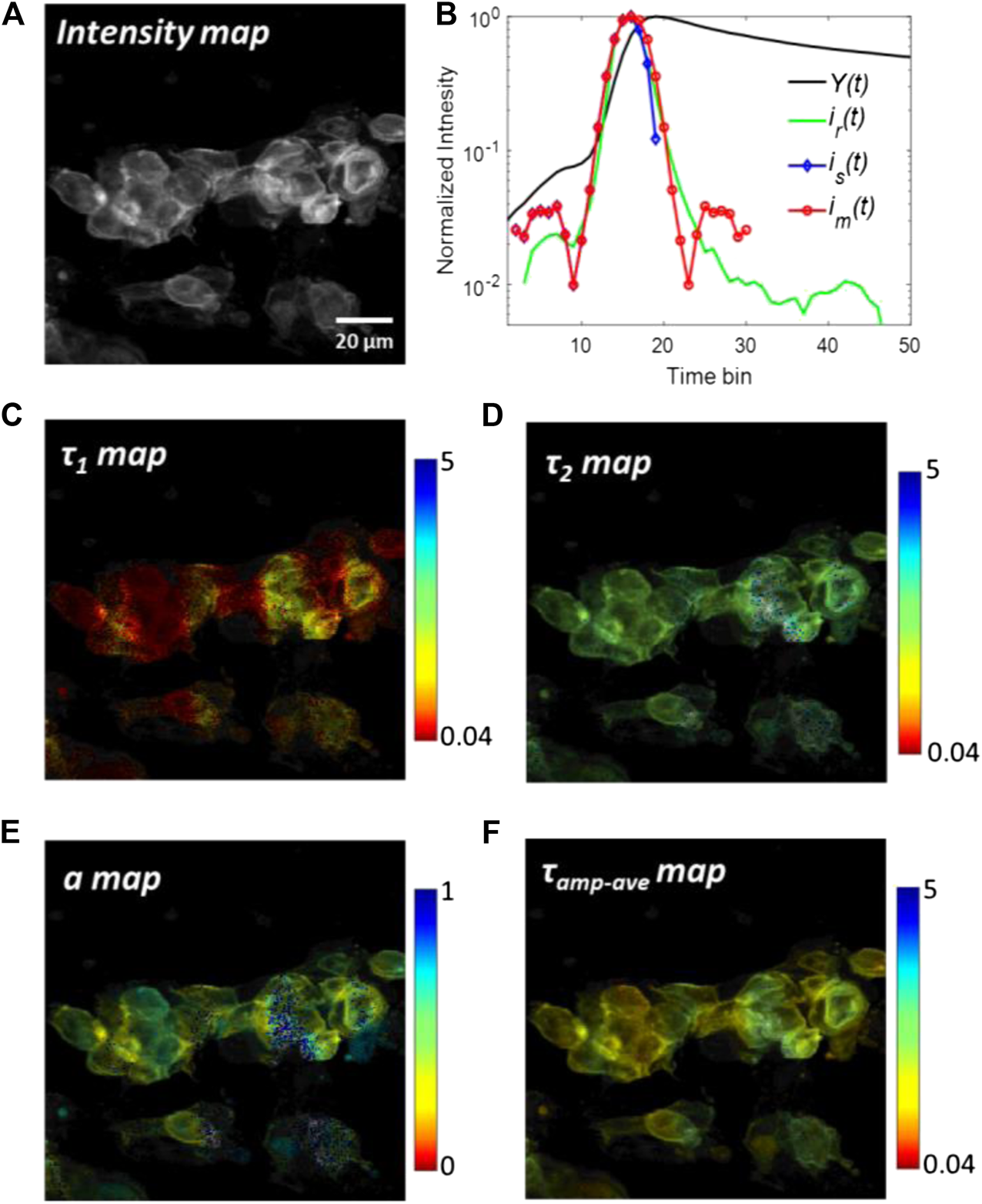
FIGURE 6. Analyzed results of tSA201 cells with co-transfected eYFP. (A) Grey-scale fluorescence intensity image. (B) Measured IRF, i_r(t), and the summed histogram, Y(t), are plotted with a green and black solid line, respectively. i_r(t) and i_m(t) are shown in dash lines with markers. (C–F)τ₁, τ₂, a, and τ_amp-ave images using the experimental IRF (i_r(t)) and constrained LSD-LE method with (α, L) = (0.92,16).

To compare the deconvolution performances of i_s(t) and i_m(t) with that of i_r(t), the corresponding lifetime images for two automatic synthetic IRFs were calculated. For a better comparison, the scatter plots of τ₁, τ₂, and two kinds of average lifetimes named amplitude-weighted average lifetime (τ_amp-ave) and intensity-weighted average lifetime (τ_int-ave) vs. α are shown in Figures 7A–D, respectively. τ_int-ave is also taken into consideration, defined as ${\tau }_{int-ave}=[a{\tau }_1^2+(1-a){\tau }_2^2]/[a{\tau }_1+(1-a){\tau }_2]$. For τ₁ and τ₂ in Figures 7A,B, it is easy to see that the lifetime distributions obtained from i_s(t) (dots with blue “+” marker) are significantly different from that of i_r(t) (green “.” marker). The clusters obtained by i_m(t) and i_s(t) are discernible. It demonstrates that the deconvolution results using i_s(t) can lead to a large bias compared to the results using i_r(t) and a wrong interpretation of the data. For example, for τ₁ with sub-nanosecond lifetime, α should be less than 0.8 according to the i_r(t) deconvolution results. Still, the results using i_s(t) leads to large dots distributions at α > 0.8 (top left corner in Figure 7A). This problem also happens for τ₂. On the other hand, for the proposed synthetic IRF i_m(t), the cluster shape of the data is almost identical with that of i_r(t), indicating that i_m(t) is more suitable for recovering the real parameters. As for the average lifetimes τ_amp-ave and τ_int-ave in Figures 7C,D, interestingly, the cluster shapes of three IRFs are similar, but the deviation of the results with i_s(t) from the other two is still noticeable. Compared to the cluster for i_r(t), the overall clusters for i_s(t) have a larger distribution range. Additionally, i_s(t) can yield an obvious artificial cluster at α = 0, which is eliminated for i_m(t). Hence, it is safe to prove that i_m(t) shows superior deconvolution performances than i_s(t). It is worth noting that, for lifetimes down to or even smaller than the FWHM of the IRF, for example, the gold nanoparticles used as the biomarkers, both the synthetic IRFs would lead to a large deviation as shown in Figure 1B. Therefore, synthetic IRFs are not suitable for deconvolution analysis. Although our synthetic can well approximate the true IRF, it does not consider the pre-pulse and sub-structure after the main peak of IRF. However, both only cause negligible effects in TCSPC measurements because their magnitudes are generally two orders smaller than the main peak.

FIGURE 7

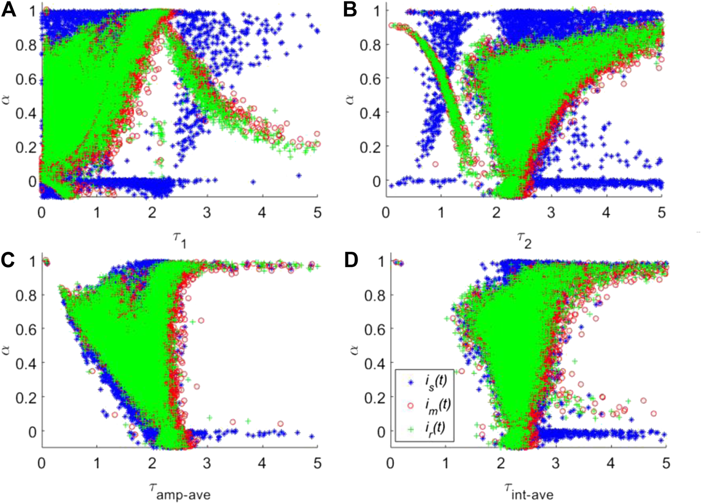
FIGURE 7. Calculated τ₁(A), τ₂(B), τ_amp-ave(C) and τ_int-ave(D) vs. α using three different IRFs, i_s(t), i_m(t) and i_r(t).

5 Conclusion

In conclusion, we proposed a strategy for obtaining the synthetic IRF of TCSPC based FLIM experiments. Compared to the simple differential synthetic IRF, the dynamic range of the mirror-symmetric synthetic IRF is significantly expanded. Even when the lifetime is close to the FWHM of the system’s true IRF, the proposed synthetic IRF can resolve the lifetime with high accuracy. At the same time, the accuracy is also much improved in the whole dynamic range. The proposed synthetic IRF was also applied to analyze bi-exponential decays with simulated data using both nonlinear least-square deconvolution and Laguerre expansion methods. The results show that the mirror-symmetric synthetic IRF has higher accuracy and a lower standard deviation. Additionally, the proposed synthetic IRF can resolve the more extended lifetime component in the whole dynamic range, unattainable in the simple differential synthetic IRF. We further investigated the proposed synthetic IRF with the real experimental FLIM-FRET data. Both simulated and experimental data show that the proposed synthetic IRF has superior performance than traditional synthetic IRF.

Data Availability Statement

The raw data supporting the conclusions of this article will be made available by the authors, without undue reservation.

Author Contributions

DX proposed the conceptualization and wrote the manuscript. MS and MC cultured and prepared the cell samples. NS and YC provided fluorescence lifetime imaging data and analysis. DL provided supervision and manuscript reviewing and editing. All authors reviewed the final manuscript.

Funding

The authors would like to acknowledge the Medical Research Scotland (1179-2017), Photon Force, Ltd., and the Engineering and Physical Sciences Research Council (EP/L01596X/1) for supporting this project. Photon Force supports the use of SPAD cameras in our project. The funder was not involved in the study design, collection, analysis, interpretation of data, the writing of this article or the decision to submit it for publication.

Conflict of Interest

The authors declare that the research was conducted in the absence of any commercial or financial relationships that could be construed as a potential conflict of interest.

References

1. Lakowicz JR. Principles of fluorescence spectroscopy. Boston, MA: Springer (2006).

Google Scholar

2. Datta R, Heaster TM, Sharick JT, Gillette AA, Skala MC. Fluorescence lifetime imaging microscopy: fundamentals and advances in instrumentation, analysis, and applications. J Biomed Opt (2020) 25(7):1. doi:10.1117/1.JBO.25.7.071203

CrossRef Full Text | Google Scholar

3. Suhling K, Hirvonen LM, Levitt JA, Chung P-H, Tregidgo C, Le Marois A, et al. Fluorescence lifetime imaging (FLIM): basic concepts and some recent developments. Med Photon (2015) 27:3–40. doi:10.1016/j.medpho.2014.12.001

CrossRef Full Text | Google Scholar

4. Ntziachristos V. Going deeper than microscopy: the optical imaging Frontier in biology. Nat Methods (2010) 7(8):603–14. doi:10.1038/nmeth.1483

PubMed Abstract | CrossRef Full Text | Google Scholar

5. Bower AJ, Sorrells JE, Li J, Marjanovic M, Barkalifa R, Boppart SA. Tracking metabolic dynamics of apoptosis with high-speed two-photon fluorescence lifetime imaging microscopy. Biomed 10(12):6408–21. doi:10.1364/BOE.10.006408

PubMed Abstract | CrossRef Full Text | Google Scholar

6. Okabe K, Inada N, Gota C, Harada Y, Funatsu T, Uchiyama S. Intracellular temperature mapping with a fluorescent polymeric thermometer and fluorescence lifetime imaging microscopy. Nat Commun (2012) 3(1):705. doi:10.1038/ncomms1714

PubMed Abstract | CrossRef Full Text | Google Scholar

7. Sagolla K, Löhmannsröben HG, Hille C. Time-resolved fluorescence microscopy for quantitative Ca2+ imaging in living cells. Anal Bioanal Chem (2013) 405(26):8525–37. doi:10.1007/s00216-013-7290-6

PubMed Abstract | CrossRef Full Text | Google Scholar

8. Schmitt FJ, Thaa B, Junghans C, Vitali M, Veit M, Friedrich T. eGFP-pHsens as a highly sensitive fluorophore for cellular pH determination by fluorescence lifetime imaging microscopy (FLIM). Biochim Biophys Acta Bioenerg (2014) 1837(9):1581–93. doi:10.1016/j.bbabio.2014.04.003

CrossRef Full Text | Google Scholar

9. Lukina MM, Shimolina LV, Kiselev NM, Zagainov VE, Komarov DV, Zagayanova EV, et al. Interrogation of tumor metabolism in tissue samples ex vivo using fluorescence lifetime imaging of NAD(P)H. Methods Appl Fluoresc (2020) 8(1):014002. doi:10.1088/2050-6120/ab4ed8

CrossRef Full Text | Google Scholar

10. Shivalingam A, Izquierdo MA, Le Marois A, Vyšniauskas A, Suhling K, Kuimova MK, et al. The interactions between a small molecule and G-quadruplexes are visualized by fluorescence lifetime imaging microscopy. Nat Commun (2015) 6(1):8178. doi:10.1038/ncomms9178

PubMed Abstract | CrossRef Full Text | Google Scholar

11. Tardif C, Nadeau G, Labrecque S, Côté D, Lavoie-Cardinal F. Fluorescence lifetime imaging nanoscopy for measuring Förster resonance energy transfer in cellular nanodomains. Neurophoton (2019) 6(1):015002. doi:10.1117/1.nph.6.1.015002

CrossRef Full Text | Google Scholar

12. Sparks H, Kondo H, Hooper S, Munro I, Kennedy G, Dunsby C, et al. Heterogeneity in tumor chromatin-doxorubicin binding revealed by in vivo fluorescence lifetime imaging confocal endomicroscopy. Nat Commun (2018) 9(1):2662. doi:10.1038/s41467-018-04820-6

PubMed Abstract | CrossRef Full Text | Google Scholar

13. Becker W. Advanced time-correlated single photon counting techniques. Berlin, Germany: Springer (2005)

Google Scholar

14. Becker W. Advanced time-correlated single photon counting applications. Berlin, Germany: Springer (2015)

Google Scholar

15. Luchowski R, Gryczynski Z, Sarkar P, Borejdo J, Szabelski M, Kapusta P, et al. Instrument response standard in time-resolved fluorescence. Rev Sci Instrum (2009) 80(3):033109. doi:10.1063/1.3095677

PubMed Abstract | CrossRef Full Text | Google Scholar

16. Chib R, Shah S, Gryczynski Z, Fudala R, Borejdo J, Zelent B, et al. Standard reference for instrument response function in fluorescence lifetime measurements in visible and near infrared. Meas Sci Technol (2016) 27(2):027001. doi:10.1088/0957-0233/27/2/027001

CrossRef Full Text | Google Scholar

17. Szabelski M, Ilijev D, Sarkar P, Luchowski R, Gryczynski Z, Kapusta P, et al. Collisional quenching of erythrosine B as a potential reference dye for impulse response function evaluation. Appl Spectrosc (2009) 63(3):363–8. doi:10.1366/000370209787598979

PubMed Abstract | CrossRef Full Text | Google Scholar

18. Szabelski M, Luchowski R, Gryczynski Z, Kapusta P, Ortmann U, Gryczynski I. Evaluation of instrument response functions for lifetime imaging detectors using quenched Rose Bengal solutions. Chem Phys Lett (2009) 471(1-3):153–9. doi:10.1016/j.cplett.2009.02.001

CrossRef Full Text | Google Scholar

19. van Oort B, Amunts A, Borst JW, van Hoek A, Nelson N, van Amerongen H, et al. Picosecond fluorescence of intact and dissolved PSI-LHCI crystals. Biophys J (2008) 95(12):5851–61. doi:10.1529/biophysj.108.140467

PubMed Abstract | CrossRef Full Text | Google Scholar

20. Wagnières GA, Star WM, Wilson BC. In vivo fluorescence spectroscopy and imaging for oncological applications. Photochem Photobiol (1998) 68(5):603–32. doi:10.1111/j.1751-1097.1998.tb02521.x

PubMed Abstract | CrossRef Full Text | Google Scholar

21. Habenicht A, Hjelm J, Mukhtar E, Bergström F, Johansson LB-Å. Two-photon excitation and time-resolved fluorescence: I. The proper response function for analysing single-photon counting experiments. Chem Phys Lett (2002) 354(5-6):367–75. doi:10.1016/s0009-2614(02)00141-0

CrossRef Full Text | Google Scholar

22. Talbot CB, Patalay R, Munro I, Warren S, Ratto F, Matteini P, et al. Application of ultrafast gold luminescence to measuring the instrument response function for multispectral multiphoton fluorescence lifetime imaging. Opt Express (2011) 19(15):13848–61. doi:10.1364/oe.19.013848

PubMed Abstract | CrossRef Full Text | Google Scholar

23.Recording the instrument response function of a multiphoton FLIM system, application note. Becker & Hickl GmbH (2008). Available from: http://www.becker-hickl.de/pdf/irf-mp04.pdf.

Google Scholar

24. Wolfgang B. The bh TCSPC Handbook. 8th ed. Available from: https://www.becker-hickl.com/literature/handbooks/the-bh-tcspc-handbook/ (Accessed September 2019).

Google Scholar

25. Digman MA, Caiolfa VR, Zamai M, Gratton E. The phasor approach to fluorescence lifetime imaging analysis. Biophys J (2008) 94(2):L14–6. doi:10.1529/biophysj.107.120154

PubMed Abstract | CrossRef Full Text | Google Scholar

26. Ranjit S, Malacrida L, Jameson DM, Gratton E. Fit-free analysis of fluorescence lifetime imaging data using the phasor approach. Nat Protoc (2018) 13(9):1979–2004. doi:10.1038/s41596-018-0026-5

PubMed Abstract | CrossRef Full Text | Google Scholar

27. Stringari C, Cinquin A, Cinquin O, Digman MA, Donovan PJ, Gratton E. Phasor approach to fluorescence lifetime microscopy distinguishes different metabolic states of germ cells in a live tissue. Proc Natl Acad Sci USA (2011) 108(33):13582–7. doi:10.1073/pnas.1108161108

PubMed Abstract | CrossRef Full Text | Google Scholar

28. Gerritsen HC, Asselbergs MA, Agronskaia AV, Van Sark WG. Fluorescence lifetime imaging in scanning microscopes: acquisition speed, photon economy and lifetime resolution. J Microsc (2002) 206(3):218–24. doi:10.1046/j.1365-2818.2002.01031.x

PubMed Abstract | CrossRef Full Text | Google Scholar

29. Li DD, Ameer-Beg S, Arlt J, Tyndall D, Walker R, Matthews DR, et al. Time-domain fluorescence lifetime imaging techniques suitable for solid-state imaging sensor arrays. Sensors (Basel) (2012) 12(5):5650–69. doi:10.3390/s120505650

PubMed Abstract | CrossRef Full Text | Google Scholar

30. Jo JA, Fang Q, Marcu L. Ultrafast method for the analysis of fluorescence lifetime imaging microscopy data based on the Laguerre expansion technique. IEEE J Sel Top Quantum Electron (2005) 11(4):835–45. doi:10.1109/JSTQE.2005.857685

CrossRef Full Text | Google Scholar

31. Jo JA, Fang Q, Papaioannou T, Marcu L. Fast model-free deconvolution of fluorescence decay for analysis of biological systems. J Biomed Opt (2004) 9(4):743–52. doi:10.1117/1.1752919

PubMed Abstract | CrossRef Full Text | Google Scholar

32. Liu J, Sun Y, Qi J, Marcu L. A novel method for fast and robust estimation of fluorescence decay dynamics using constrained least-squares deconvolution with Laguerre expansion. Phys Med Biol (2012) 57(4):843–65. doi:10.1088/0031-9155/57/4/843

PubMed Abstract | CrossRef Full Text | Google Scholar

33. Pande P, Jo JA. Automated analysis of fluorescence lifetime imaging microscopy (FLIM) data based on the Laguerre deconvolution method. IEEE Trans Biomed Eng (2011) 58(1):172–81. doi:10.1109/TBME.2010.2084086

PubMed Abstract | CrossRef Full Text | Google Scholar

34. Zhang Y, Chen Y, Chen Y, Li DD. Optimizing Laguerre expansion based deconvolution methods for analysing bi-exponential fluorescence lifetime images. Opt Express (2016) 24(13):13894–905. doi:10.1364/OE.24.013894

PubMed Abstract | CrossRef Full Text | Google Scholar