Event-Chain Monte-Carlo Simulations of Dense Soft Matter Systems

1 Event-Chain Monte-Carlo Algorithm

Since its first application to a hard disk system [1], Monte-Carlo (MC) simulations have been applied to virtually all types of models in statistical physics, both on-lattice and off-lattice. MC samples microstates $\left\{a,b,\dots \right\}$ of a thermodynamic ensemble statistically according to their Boltzmann weight ${\pi }_a=\text{exp}\left(-E_a/k_{B}T\right)$ (in the following, we use thermal units, k_BT = 1). One advantage of MC schemes over, for example molecular dynamics simulations, is that it only requires knowledge of microstate energies E_a rather than interaction forces. In its simplest form, the Metropolis-Hastings algorithm [1, 2], a MC simulation is easily implemented for any system by offering moves from a microstate a to a microstate b of the system and accepting or rejecting these moves according to the Metropolis rule for the Boltzmann distribution, i.e., based on the energy difference between states $\Delta E_{a\to b}=E_b-E_a$. The standard Metropolis rule is defined by the acceptance probability

$p^{\text{Metr}}\left(a\to b\right)=\min \left(1,\frac{{\pi }_b}{{\pi }_a}\right)=\min \left(1,\exp \left(-\Delta E_{a\to b}\right)\right)=\exp \left(-{\left[\Delta E_{a\to b}\right]}^{+}\right)(1)$

$\text{with} {\left[x\right]}^{+}\equiv \max \left(0,x\right)$

for a move $a\to b$. Together with the trial probability $p^{\text{trial}}\left(a\to b\right)$ that a move $a\to b$ is proposed we obtain the transition rate as the product $p\left(a\to b\right)=p^{\text{trial}}\left(a\to b\right)p^{\text{Metr}}\left(a\to b\right)$. The transition rates $p\left(a\to b\right)$ give rise to probability currents $J_{a\to b}={\pi }_{a}p\left(a\to b\right)$ from state a to b. Transition rates $p\left(a\to b\right)$ are given per MC time; likewise probability currents $J_{a\to b}$ have units probability per MC time, which must not be identified with an actual physical time. The Metropolis rule is designed to fulfill detailed balance of probability currents between any states a and b, i.e.,

$J_{a\to b}={\pi }_{a}p\left(a\to b\right)={\pi }_{b}p\left(b\to a\right)=J_{b\to a}.(2)$

The Metropolis rule (1) satisfies detailed balance for the Boltzmann distribution ${\pi }_a=\text{exp}\left(-E_a\right)$ if moves are also offered with a symmetric trial probability $p^{\text{trial}}\left(a\to b\right)=p^{\text{trial}}\left(b\to a\right)$ (which is typically fulfilled trivially for standard local MC moves). A characteristic of the Metropolis rule (1) is also that moves that are energetically downhill, $\text{Δ}{E}_{a\to b}<0$, are always accepted ($p^{\text{Metr}}\left(a\to b\right)=1$). We point out that detailed balance (for symmetric trial probabilities) and this maximal acceptance rate for energetically downhill moves determine the Metropolis rule for the Boltzmann distribution uniquely. The Metropolis acceptance rate for moves that are energetically uphill is exponentially small, however, resulting in frequent rejections.

Typical local MC moves, such as single spin flips in spin systems or single particle moves in off-lattice systems of interacting particles, are often motivated by the actual dynamics of the system. Sampling with local moves can become slow, however, in certain physically relevant situations, most notably, close to a critical point, where large correlated regions exist, or in dense systems, where acceptable moves become rare.

Cluster algorithms deviate from the local Metropolis MC rule and construct MC moves of large non-local clusters, ideally, in a way that the MC move of the cluster is performed rejection-free. For lattice spin systems, the Swendsen-Wang [3] and Wolff [4] algorithms are the most important cluster algorithms with enormous performance gains close to criticality, where they reduce the dynamical exponent governing the critical slowing down in comparison to local MC simulations. These cluster algorithms still fulfill detailed balance but based on a non-trivial trial probability that derives from the cluster construction rules.

The event-chain (EC) MC algorithm introduced by Krauth et al. [5] has been developed to decrease the autocorrelation time in hard disk or sphere systems. It performs rejection-free displacements of several spheres in a single MC move (see Figure 1) and can, therefore, also be classified as a cluster algorithm. The basic idea is to perform a displacement $\ell$ in a billiard-type fashion, transferring the displacement to the next disk upon a collision, which is called an event and gives the algorithm its name (see Figure 1). As opposed to cluster algorithms such as the Swendsen-Wang or Wolff algorithms, ECMC algorithms do no longer fulfill detailed balance but only global balance.

FIGURE 1

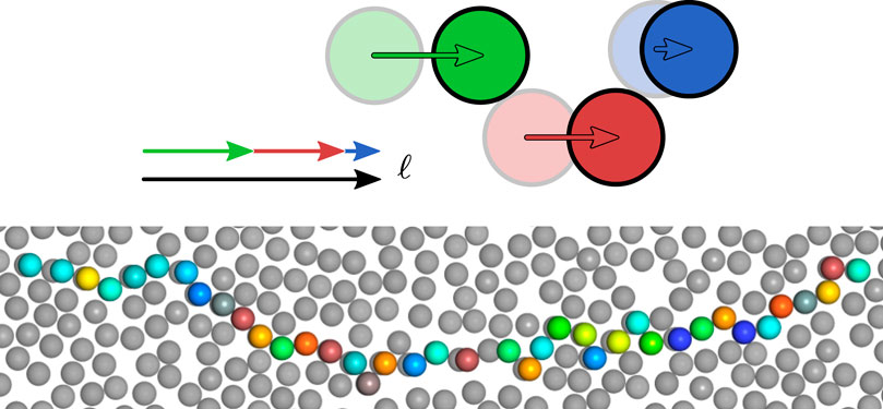
FIGURE 1. The upper scheme illustrates the billiard-type construction of an EC with a total displacement length $\ell$ and with three participating spheres. The lower picture shows the example of a typical EC in a dense hard-sphere system: the coherent movement of long line-like clusters in each ECMC move accelerates the sampling by nearly two orders of magnitude.

In the following, we will give an introduction into the ECMC algorithm starting with the example of simple hard sphere systems. We then discuss how the algorithm realizes the general concept of lifting moves, which is employed in order to achieve global balance. Finally, we review the adaptation and generalization of the ECMC algorithm from athermal systems with hard interactions to systems with soft potentials specified by an interaction energy. Many soft matter systems can be constructed from hard spheres as basic building blocks, eventually with additional interactions, for example spring-like connections to form a polymer chain. We discuss in some detail several applications of the EC algorithm in dense soft matter systems, namely polymer systems, liquid crystal systems as well as mixed systems such as liquid crystal colloids.

1.1 EC Algorithm for Hard Spheres

We consider the conceptually simple system of hard (impenetrable) disks (of diameter σ) in two dimensions in order to introduce the ECMC algorithm. Hard disks are the epitome of a system that is easily described and quickly implemented in a (naive) simulation [1], but exhibits a non-trivial phase transition that has been debated for a long time [6]. The two-dimensional melting phase transition is believed to be a two-step Kosterlitz-Thouless melting via an intermediate hexatic phase [7–9], which is, however, difficult to confirm unambiguously in simulations [10, 11].

In a hard disk system, an EC move is constructed by first selecting a random starting particle, an EC displacement direction, and a total displacement length $\ell$. Both direction and total displacement length $\ell$ are adjustable parameters of the algorithm (see Figure 1); the sampling of EC directions of directions (uniform or non-uniform) will determine whether detailed or global balance is fulfilled, while the displacement length $\ell$ can be adjusted for performance. We start the EC by moving the chosen particle in the EC direction, which is only possible until it touches another particle after a certain displacement r, which will be typically much smaller than the intended displacement $\ell$ in a dense system. Then, instead of declining such a move as in local MC schemes, the displacement r of the first particle is subtracted from the initial total displacement length and the remaining displacement $\ell -r$ is carried over to the hit particle, which we attempt to displace next by the remaining distance $\ell -r$. If also the displacement direction is carried over to the hit particle the EC is called straight; this is the case we will focus on in the following and which is illustrated in Figure 1. This procedure of lifting the EC to the next particle upon collision continues until no displacement length is left. Then an EC has been constructed that moved as a line-like cluster without the possibility of rejection, and we start over by choosing a new starting particle and a new random starting direction to construct the next EC with the same total displacement length $\ell$.

The total displacement length $\ell$ is an adjustable algorithm parameter, which determines the average number of disks $n_{\text{EC}}$ that are moved in an EC move (see Figure 1). This number is given by $n_{\text{EC}}\sim \ell /{\lambda }_0$, where ${\lambda }_0$ denotes the mean free path; in general, the efficiency of the EC algorithm depends crucially on $n_{\text{EC}}$. For smaller $\ell$, the efficiency decreases and approaches traditional local MC (corresponding to the case $\ell <{\lambda }_0$). For very large $\ell$, ECs comprise large parts of the system and give rise to motion similar to a collective translation of disks, which is also inefficient.

We note that the EC algorithm will be very well suited to simulate dense systems but does not allow to simulate maximally dense, i.e., jammed systems since an EC can not displace any particle if all particles touch each other. In jammed hard disk systems, the mean free path ${\lambda }_0$ approaches zero such that the number of participating disks $n_{\text{EC}}$ diverges, and the EC does no longer terminate or essentially comprises the entire system resulting in collective translation. This will happen for $n_{\text{EC}}\sim \ell /{\lambda }_0>N$. In a dense hard disk system of area $L^2$ and close to the close-packing volume fraction ${\eta }_{hcp}=\pi /2\sqrt{3}$, we have ${\lambda }_0\approx \sigma \left({\eta }_{hcp}-\eta \right)/2{\eta }_{hcp}$ resulting in a more concrete condition $\ell \mathrm{\lesssim }\left({\eta }_{hcp}-\eta \right)L^2/\sigma$ for the EC algorithm to remain effective close to close-packing.

We will show in the next section that the EC algorithm ensures global balance, regardless of how the EC displacement direction is chosen. If the EC displacement directions are chosen randomly the straight EC algorithm also satisfies detailed balance over many EC events. The most performant version of the straight EC algorithm, however, the so-called xy-version or irreversible straight EC algorithm, breaks detailed balance and uses only displacements along coordinate axes and only in positive direction. Breaking detailed balance but preserving global balance leads to performance gains. Ergodicity must also be ensured, which is done via periodic boundary conditions for the irreversible EC algorithm; moreover, several computations can be simplified for the xy EC algorithm. In Ref. [12], the irreversible EC simulations are roughly 70 times faster than a simulation employing local MC moves. We can obtain similar performance gains in dense soft matter systems.

1.2 Balance Conditions and Lifting for Hard Spheres

The standard Metropolis algorithm (1) employs detailed balance to ensure stationarity of the probability distribution of states by pairwise balancing of probability fluxes between microstates in condition (2). Since circular probability fluxes also fulfill the stationarity requirement for the probability distribution, detailed balance is not a necessary condition and, often, performance can be gained by finding an algorithm that fulfills the weaker condition of global balance,

${\displaystyle \sum }_b{J}_{b\to a}={\displaystyle \sum }_b{\pi }_{b}p\left(b\to a\right)={\pi }_a{\displaystyle \sum }_{c}p\left(a\to c\right)={\displaystyle \sum }_c{J}_{a\to c}={\pi }_a(3)$

(where the sums are over all microstates), which is simply the continuity equation for a stationary probability ${\pi }_a$, i.e., the Boltzmann distribution in our case. While the last equality in Eq. 3 is a trivial consequence of normalization, the second equality is the actual global balance condition. All quantities in Eq. 3 are transition probabilities per MC step; we call the algorithmic time measured in MC steps τ in the following. The algorithmic time τ measured in MC steps must not be identified with an actual physical time t as for any MC simulation.

Global balance algorithms should become particularly performant if maximal global balance is achieved, which means that probability backflow is forbidden leading to the additional constraint

$J_{a\to b}\ne 0\Rightarrow J_{b\to a}=0.(4)$

In particular, this implies a rejection-free algorithm, i.e., $J_{a\to a}=0$. Then we can also take a hydrodynamic point of view and see probability density as liquid mass density, unidirectional transition probabilities as liquid velocities, and the probability currents as liquid current densities. Then, maximal global balance corresponds to stationarity of the mass distribution in the presence of fluid flow, i.e., a divergence-free liquid current density.

In Figure 2, we show how maximal global balance is achieved in EC algorithms for a hard sphere system. In order to investigate balance conditions, it is often convenient to decompose the EC into infinitesimal moves $dw$, which add up to the total EC displacement $\ell$ in the end [13–15]. To ensure maximal global balance lifting transitions are introduced, which change an additional lifting variable that enlarges the state space of the system [16]. For hard sphere systems, the additional lifting variable is simply the number i of the active/moving particle. This will be the case throughout this article. The microstates are then characterized not only by the positions of all particles but also by specifying the active particle.

FIGURE 2

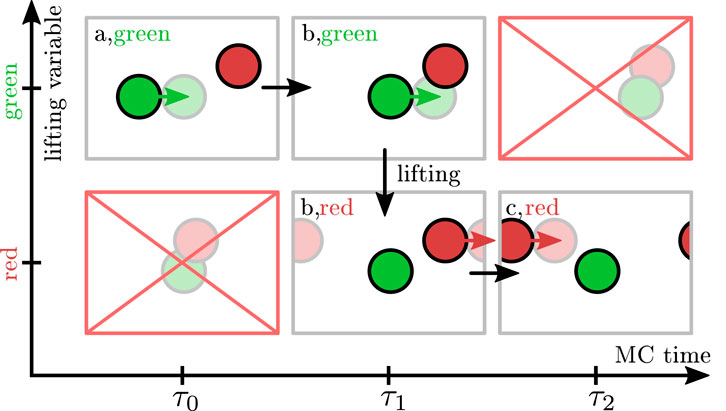
FIGURE 2. Scheme of the lifting formalism for hard spheres. The physical states are labeled with letters (a,b,c) and the lifting variable is indicated by color, i.e., the current active particle is indicated by a colored arrow. The EC displacement direction is to the right. Proposed infinitesimal displacements are indicated by opaque spheres. In case of a physical rejection at MC step ${\tau }_1$ the pivot particle is changed and rejection is avoided. Periodic boundaries ensure ergodicity. One way to read this scheme, is that the lower row is the displacement-reversed version (except trivial translations) of the upper row (obtained be reversing all displacements $dw\to -dw$), resulting in a central symmetry, especially (c,red) $=$ (a,green).

For infinitesimal EC moves, only two spheres can collide at once, and it is sufficient to consider a simplified setting of only two hard spheres (green and red) as shown in the cartoon in Figure 2, where proposed infinitesimal displacements are indicated by opaque spheres. The physical states are labeled with letters (A and b,c), and the lifting variable is indicated by color (red or green particle is active). Physical transitions change the physical states by changing particle positions; this happens by moving the active sphere in the EC displacement direction (i.e., to the right from (a,green) at ${\tau }_0$ to (b,green) at ${\tau }_1$ in Figure 2). If a physical transition leads to an overlap, instead of rejecting the move as in local MC, we perform a lifting transition and change the lifting variable with a lifting probability that exactly equals the rejection probability of the local MC rule in the EC algorithm. In Figure 2), this means that the active particle is changed to the red sphere if a collision is proposed at ${\tau }_1$. Then the red active particle continues to move (to the right from (b,red) to (c,red).

In this way, rejections are avoided, and the entire rejection probability flow is redirected to a lifting move probability flow, which ensures maximal global balance if all physical configurations are equally probable, i.e., if the Boltzmann distribution for hard spheres holds:

The total physical inflow $J_{\text{a},\text{green}\to \text{b},\text{green}}^{\text{phys}}$ to (b,green) equals the rejected physical flow $J_{\text{b},\text{green}\to \text{coll}}^{\text{phys}}$ (that would lead to collisions on the upper right picture) because it involves moving the same sphere by the same distance $dw$ and because physical states a and b are equally probable.

By construction of the EC algorithm, all collisions give rise to lifting such that the lifting flow $J_{\text{b},\text{green}\to \text{b},\text{red}}^{\text{lift}}$ equals the rejected physical flow $J_{\text{b},\text{green}\to \text{coll}}^{\text{phys}}$. This leads to $J_{\text{a},\text{green}\to \text{b},\text{green}}^{\text{phys}}=J_{\text{b},\text{green}\to \text{b},\text{red}}^{\text{lift}}$, so far.

Apart from a translation, the states a and c and the forbidden overlapping configurations (upper right and lower left pictures in Figure 2) are identical (please note the periodic boundary conditions).

Therefore, the missing physical inflow $J_{\text{coll}\to \text{b},\text{red}}^{\text{phys}}$ (from the forbidden overlapping configuration on the lower left picture) into state (b,red) equals the rejected physical flow $J_{\text{b},\text{green}\to \text{coll}}^{\text{phys}}$ and, thus, the lifting flow $J_{\text{b},\text{green}\to \text{b},\text{red}}^{\text{lift}}$.

Again, the missing physical inflow $J_{\text{coll}\to \text{b},\text{red}}^{\text{phys}}$ into state (b,red) equals the physical outflow $J_{\text{b},\text{red}\to \text{c},\text{red}}^{\text{phys}}$ from (b,red) because it involves moving the same sphere by the same distance $dw$ and because physical states b and c are equally probable.

All in all, we obtain

$J_{\text{a},\text{green}\to \text{b},\text{green}}^{\text{phys}}=J_{\text{b},\text{green}\to \text{b},\text{red}}^{\text{lift}}=J_{\text{b},\text{red}\to \text{c},\text{red}}^{\text{phys}},$

which are exactly the maximal global balance conditions for states (b,green) and (b,red) proving maximal global balance for any EC move on a state space that is extended by the lifting variable denoting the active particle. Global balance holds, regardless of how the EC displacement direction or displacement length is chosen. If the reverse EC displacement directions are offered with the same probability (for example by drawing EC directions completely uniformly in all directions) the resulting EC algorithm also satisfies detailed balance over the course of many EC moves.

For pair interactions between hard spheres the lifting variable is the particle number. We can also introduce hard walls to the system, which represent additional steric one-particle interactions. For such one-particle interactions, the lifting variable will not be the particle number (as there are no interaction partners, the active particle must stay the same) but the EC direction itself. It can be shown that classical reflection of the EC direction upon collision with the hard wall will ensure maximal global balance. Analogously to the forbidden overlapping configurations Figure 2, both the rejected outflow in a collision with a wall and the missing inflow from forbidden configurations are exactly equal to the lifting flow from reflected EC directions.

1.3 Soft Interaction Energies

In many applications other than pure hard core systems, we have to deal with systems containing hard core repulsion alongside with other soft interaction energies $\mathrm{ℰ}=\mathrm{ℰ}\left({\mathbf{r}}_1,\dots ,{\mathbf{r}}_N\right)$ that can depend on all particle positions ${\mathbf{r}}_n$ in a canonical ensemble. These are not handled by the hard sphere EC scheme described so far. One naive strategy to handle an additional interaction is the following: to ensure ergodicity, an EC is limited to a total displacement $\ell$, i.e., the sum of all particle displacements, after which a random new particle is chosen as active and a new isotropic direction is set. Interpreting a whole EC as a single MC move, an additional interaction will cause an energy change $\text{Δ}\mathrm{ℰ}$ when a hard sphere EC (which ignores the additional soft interaction) is executed. To properly sample the Boltzmann distribution in the presence of the additional interaction, the EC as a whole is then accepted or rejected by a standard Metropolis filter (1).

This strategy of handling additional interaction energies by re-introduction of Metropolis sampling and, thus, rejections will surely decrease the efficiency of the simulation. All advantages of the EC algorithm are effectively lost. There is, however, a way to include arbitrary $\mathcal{N}$-particle interaction energies into the EC framework. Within the lifting formalism it is possible to extend the algorithm from hard spheres to arbitrary pair potentials and continuous spin models by employing factorized Metropolis filters [13, 17, 18]; this concept can be further generalized to $\mathcal{N}$-particle interactions with $\mathcal{N}>2$ according to Ref. [15]. In principle, these expansions of the EC algorithm presented in the following can be reduced to our simple example of a two-sphere collision from Figure 2 by generalizing the notion of a collision [17]. Effectively, we assign a virtual hard sphere radius to each interaction, which determines which configurations are energetically forbidden and trigger a generalized collision. This can be done by introducing the so-called rejection distance, which is further explained in Figure 4.

In a pure hard sphere simulation, a sphere is continuously displaced until it hits another sphere which triggers a lifting event (or the total displacement reaches $\ell$). We can resolve all events into unique binary collisions or rejections, which then leads to a simple lifting probability flux during each event (see Figure 2). When a particle is displaced in the presence of continuous interaction energies, it is not clear which interaction causes the rejection, since the rejection in the standard Metropolis filter is based on the sum of all changes in all interaction energies (pair or many-particle interactions). In fact, the rejection is caused by all interactions at once. By using an infinitesimal factorized Metropolis filter one can handle each interaction independently.

Each particle i has a set $S_i$ of interactions with other particles; each interaction energy $\mathrm{ℰ}\in S_i$ depends on the position ${\mathbf{r}}_i$ of particle i and on the positions of other particles in the set $M_{\mathrm{ℰ}}$ of interaction partners participating in $\mathrm{ℰ}$. Pairwise interactions, such as elastic springs $\mathrm{ℰ}=E_{\text{spring}}\left(ij\right)$ in a bead-spring polymer or a van-der-Waals interaction between particles, are interactions with one other particle j ($M_{E_{\text{spring}}\left(ij\right)}=\left\{j\right\}$; all particles $j\ne i$ can be interaction partners); three-particle interactions such as a bending energy in a polymer are interactions $\mathrm{ℰ}=E_{\text{bend}}\left(jik\right)$ with two other particles $j,k$ that form two neighboring bonds with i and thus define a bond angle ($M_{E_{\text{bend}}\left(ijk\right)}=\left\{j,k\right\}$; all pairs $jk$ with $j\ne i,k\ne i$ can be interaction partners).

In the following, we consider again infinitesimal displacements $dw$ of particle i in the EC direction. Such an infinitesimal move changes the configuration from b to a and leads to the total energy change $d{E}_{i,b\to a}$, which is the sum of all changes in interactions in $S_i$, $d{E}_{i,b\to a}={\displaystyle \sum }_{\mathrm{ℰ}\in S_i}d{\mathrm{ℰ}}_{i,b\to a}$.

We construct a global balance algorithm starting from a Metropolis filter for the acceptance of physical moves based on the energy $d{E}_{i,b\to a}$. For soft interactions we switch, however, from the standard Metropolis filter (1) to a factorized one [13, 17, 18], where the Boltzmann weights for the sum $d{E}_{i,b\to a}={\displaystyle \sum }_{\mathrm{ℰ}\in S_i}d{\mathrm{ℰ}}_{i,b\to a}$ are factorized and the Metropolis acceptance rule is applied to each factor separately. This is equivalent to switching the sum and maximum operation on the energy changes regarding each interaction,

$p^{\text{fact}}\left(i,b\to a\right)=\text{exp}\left(-{\displaystyle \sum }_{\mathrm{ℰ}\in S_i}{\left[d{\mathrm{ℰ}}_{i,b\to a}\right]}^{+}\right)\approx 1-{\displaystyle \sum }_{\mathrm{ℰ}\in S_i}{\left[d{\mathrm{ℰ}}_{i,b\to a}\right]}^{+}.(5)$

It will be important that the factorized Metropolis filter still has the detailed balance property (2). The probability of rejecting the next infinitesimal step $1-p^{\text{fact}}$ is proportional to the sum of each infinitesimal energy change of each interaction. If one interaction causes a rejection, the whole move is rejected. Since we employ infinitesimal steps, only one interaction can reject at once. In analogy to the hard sphere case, these rejection events can be seen as a generalized collision events. In other words, the factorized Metropolis filter uniquely assigns a rejection to one specific interaction at the expense of an increased rejection rate, because energy increase from one interaction cannot be compensated by an energy decrease of another interaction.

The factorized Metropolis filter can now be used to construct a maximal global balance algorithm on an enlarged state space by redirecting all physical rejection events into lifting events. This is done analogously to the hard sphere case outlined above. If a rejection should take place according to the factorized Metropolis filter, we perform a compensating lifting move instead. We lift to one of the particles that participate in the interaction that caused the rejection. For a pair interaction this already determines the particle to lift to uniquely, for many-body interactions an additional rule is needed to select the particle to lift to properly [15]. Therefore, we first discuss the simpler case of pair interactions and show how we can realize maximal global balance.

1.3.1 Pair Interactions

For states in the enlarged state space, we use the notation $a_i$ for a physical state a with an active particle i. In the following we try to move the active particle i by an infinitesimal step $dw$ along the EC direction $\mathbf{d}$ resulting in a physical move from $a_i$ into $b_i$. For pairwise interactions $\mathrm{ℰ}\left(ij\right)$ (i.e., $S_i=\left\{\mathrm{ℰ}\left(ij\right)\right|j\ne i\}$) the transition rate is given by the factorized Metropolis filter

$p^{\text{phys}}\left(a_i\to b_i\right)=p^{\text{fact}}\left(i,a\to b\right)=\text{exp}\left(-{\displaystyle \sum }_{\mathrm{ℰ}\in S_i}{\left[-d{\mathrm{ℰ}}_{a_i\to b_i}\left(ij\right)\right]}^{+}\right)\approx 1-{\displaystyle \sum }_{\mathrm{ℰ}\in S_i}{\left[-d{\mathrm{ℰ}}_{a_i\to b_i}\left(ij\right)\right]}^{+}.(6)$

This transition rate is decreased by rejections if a move has $d{\mathrm{ℰ}}_{a_i\to b_i}\left(ij\right)>0$, i.e., is energetically uphill. If $p^{\text{phys}}\left(a_i\to b_i\right)>0$ because configuration $b_i$ can be reached by a move $dw$ of particle i from $a_i$, it follows that $p^{\text{phys}}\left(b_i\to a_i\right)=0$ because the EC direction is fixed, and we cannot reach $a_i$ from $b_i$ by moving i into the same direction $dw$ (we would need to move into the opposite direction $-dw$). Therefore, physical transitions are unidirectional.

Because only one pair interaction $\mathrm{ℰ}\left(ij\right)$ can reject at once in the factorized Metropolis filter, it is sufficient to consider the two interacting particles i and j in deriving the lifting probabilities $p_{\mathrm{ℰ}\left(ij\right)}^{\text{lift}}\left(b_i\to b_j|a_i\to b_i\right)$ from global balance, see Figure 3. We want to apply the global balance condition (3) to incoming physical and lifting flows to state $b_i$. Using detailed balance of the factorized Metropolis filter we obtain for the physical inflow from $a_i$ to $b_i$

$J_{a_i\to b_i}^{\text{phys}}={\pi }_{a_i}{p}^{\text{fact}}\left(i,a\to b\right)={\pi }_{b_i}{p}^{\text{fact}}\left(i,b\to a\right)={\pi }_{b_i}\left(1-{\left[-d{\mathrm{ℰ}}_{a_i\to b_i}\left(ij\right)\right]}^{+}\right)(7)$

Lifting moves from $b_j$ to $b_i$ are triggered by a move $dw$ of particle j into configuration $b_j$ from a different configuration $c_j$, which is obtained from $b_j$ by displacing particle j by $-dw$ ($c_j$ is analogous to the forbidden configuration on the lower left in Figure 2).

$J_{b_j\to b_i}^{\text{lift}}={\pi }_{b_j}{p}_{\mathrm{ℰ}\left(ij\right)}^{\text{lift}}\left(b_j\to b_i|c_j\to b_j\right)={\pi }_{b_i}{p}_{\mathrm{ℰ}\left(ij\right)}^{\text{lift}}\left(b_j\to b_i|c_j\to b_j\right)(8)$

with ${\pi }_{b_i}={\pi }_{b_j}={\pi }_b/N$ by symmetry in a N-particle system. Using the global balance condition (3) for flows to state $b_i$,

$J_{a_i\to b_i}^{\text{phys}}+J_{b_j\to b_i}^{\text{lift}}={\pi }_{b_i},(9)$

and dividing by ${\pi }_{b_i}$ we obtain the lifting probability as

$p_{\mathrm{ℰ}\left(ij\right)}^{\text{lift}}\left(b_j\to b_i|c_j\to b_j\right)={\left[-d{\mathrm{ℰ}}_{a_i\to b_i}\left(ij\right)\right]}^{+}={\left[d{\mathrm{ℰ}}_{c_j\to b_j}\left(ij\right)\right]}^{+}.(10)$

FIGURE 3

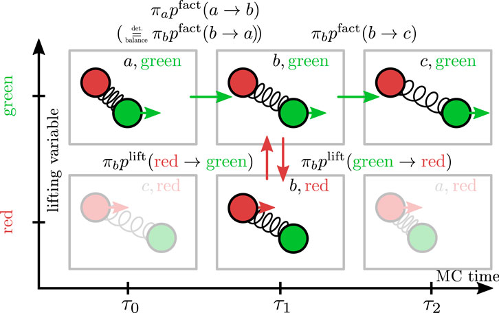
FIGURE 3. Scheme of the lifting formalism for a continuous pair interaction (notation see Figure 2). Using Eq. 5 in the global balance condition (3) for incoming and outgoing currents for state b and dividing by ${\pi }_b$ yields $p^{\text{lift}}(\text{red}\to \text{green})-{\left[d{\mathrm{ℰ}}_{b\to c}\right]}^{+}=p^{\text{lift}}(\text{green}\to \text{red})-\left[d{\mathrm{ℰ}}_{b\to a}\right]$, where $d{\mathrm{ℰ}}_{b\to c}=-d{\mathrm{ℰ}}_{b\to a}\equiv d\mathrm{ℰ}$ because of translational invariance. ${\left[d\mathrm{ℰ}\right]}^{+}=0$ leads to $p^{\text{lift}}(\text{red}\to \text{green})=0$, yielding $p^{\text{lift}}(\text{green}\to \text{red})={[-d\mathrm{ℰ}]}^{+}$ and vice versa, which assures maximal global balance. Detailed balance for physical transitions (green) ensures time reversibility, so that a reversed EC would redo the original one, while an EC itself satisfies maximal global balance. For clarity we completed the lower row to show translational symmetry.

The last equality holds for a translationally invariant pair interaction, where $d{\mathrm{ℰ}}_{c_j\to b_j}\left(ij\right)=-d{\mathrm{ℰ}}_{a_i\to b_i}\left(ij\right)$. In the other lifting direction, this implies

$p_{\mathrm{ℰ}\left(ij\right)}^{\text{lift}}\left(b_i\to b_j|a_i\to b_i\right)={\left[d{\mathrm{ℰ}}_{a_i\to b_i}\left(ij\right)\right]}^{+},(11)$

which leads to a rejection-free algorithm because the rejection probability of the physical moves (6) is exactly redirected into a lifting probability. We also conclude that $p_{\mathrm{ℰ}\left(ij\right)}^{\text{lift}}\left(b_j\to b_i\right)>0$ requires $p_{\mathrm{ℰ}\left(ij\right)}^{\text{lift}}\left(b_i\to b_j\right)=0$, i.e., also lifting transitions are unidirectional proving maximal global balance.

Global balance is established for each move $a_i\to b_i$ independently This generalizes the picture from Figure 2 to soft interactions. In fact, for hard spheres ${\left[d{\mathrm{ℰ}}_{a_i\to b_i}\left(ij\right)\right]}^{+}=0$ before a collision and ${\left[d{\mathrm{ℰ}}_{a_i\to b_i}\left(ij\right)\right]}^{+}=\infty$ at collision such that lifting to the colliding particle j happens with probability one upon collision, exactly as in Figure 2.

For an efficient implementation, an event-based approach is chosen [13, 17], in which we determine the distance to the next rejection. This rejection distance corresponds to the distance to the next collision for hard spheres.

The probability $p\left(w_{ij}\right)$ to reject and lift from particle i to particle j because of the interaction $\mathrm{ℰ}\left(ij\right)$ and after moving a distance in the interval $\left[w_{ij},w_{ij}+dw\right]$ is given by the probability to not encounter a rejection/lifting up to $w_{ij}$ and then lift with probability $p_{\mathrm{ℰ}\left(ij\right)}^{\text{lift}}\left(w_{ij}\right)dw={\left[d{\mathrm{ℰ}}_{a_i\to b_i}\left(ij,w_{ij}\right)\right]}^{+}$, see Eq. 11. As a result, we obtain a Poisson-type distribution for the rejection distance $w_{ij}$ of particle i caused by interactions with particle j,

$p\left(w_{ij}\right)=\text{exp}\left(-{{{\displaystyle \int }}^{\text{}}}_0^{w_{ij}}dw{\left[{\partial }_w\mathrm{ℰ}\left(ij,w\right)\right]}^{+}\right){\left[{\partial }_w\mathrm{ℰ}\left(ij,w_{ij}\right)\right]}^{+},(12)$

which depends on all uphill energy differences caused by particle j if particle i is moved, see Figure 4. Interpreting $-{\partial }_w\mathrm{ℰ}\left(ij,w\right)$ as force onto particle i exerted by particle j, the rejection length distribution depends on the line integral over all opposing forces.

FIGURE 4

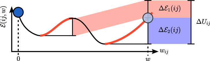
FIGURE 4. Event-driven approach to determine the rejection distance for a pair interaction between i and j. Condition (13) has to be solved for the rejection distance $w_{ij}$ at which an event/lifting occurs. The black curve is the interaction energy along the EC direction. Only on red segments with increasing energy a rejection can occur. Among all pair interactions, the rejection will be assigned to the interaction with the smallest rejection distance.

Transforming the probability distribution Eq. 12, we find that the distribution of the usable (i.e., uphill) energy $\text{Δ}{U}_{ij}={{{\displaystyle \int }}^{\text{}}}_0^{w_{ij}}dw{\left[{\partial }_w\mathrm{ℰ}\left(ij,w\right)\right]}^{+}$ is a simple exponential. It follows that the lifting distance $w_{ij}$ caused by particle j can be determined with the proper distribution by drawing a probability $u_{ij}=p\left(\text{Δ}{U}_{ij}\right)$ from a uniform distribution in $\left[\mathrm{0,1}\right]$, which translates into an exponentially distributed $\text{Δ}{U}_{ij}=-\text{ln}{u}_{ij}$, and by solving the equation

$-\text{ln}{u}_{ij}=\text{Δ}{U}_{ij}={{{\displaystyle \int }}^{\text{}}}_0^{w_{ij}}dw{\left[{\partial }_w\mathrm{ℰ}\left(ij,w\right)\right]}^{+}(13)$

for $w_{ij}$. This is illustrated in Figure 4. Because all interaction energies $\mathrm{ℰ}\left(ij\right)$ with different partners j are independent, rejection probabilities from the factorized Metropolis filter are additive by construction, and we have a Poissonian rejection length distribution, we can determine a rejection distance for all possible interaction energies, and the shortest distance triggers the next lifting event. This is analogous to the first-reaction method in a Gillespie algorithm [19]. In this sense, the rejection distance is a virtual collision radius, which can be assigned to each interaction, and the shortest collision radius triggers a generalized collision. This procedure based on (13) gives a simple and fast event-driven ECMC algorithm for arbitrary pair potentials.

1.3.2 $\mathcal{N}$-Particle Interactions

In many applications, also three-particle interactions occur. This happens, in particular, for extended objects, such as rods or polymers, which can be described by bead-spring models. One prominent example are semiflexible polymer chains with a bending energy. Because the local bending angle involves three neighboring beads in a discrete model, the bending energy is a three-particle intra-polymer interaction in terms of bead positions.

In Ref. [15], the EC algorithm has been generalized to three- and many-particle interactions, thus broadening the range of applicability of rejection-free EC algorithms considerably. For $\mathcal{N}$-particle interactions $\mathrm{ℰ}$, there are $\mathcal{N}-1$ interacting particles to which the EC can lift to avoid rejections.

In order to redirect the rejection probability ${\left[d{\mathrm{ℰ}}_{a_i\to b_i}\right]}^{+}$ from physical moves into lifting moves and, thus, a rejection-free algorithm, lifting to the set $M_{\mathrm{ℰ}}$ of $\mathcal{N}-1$ interaction partners should be done with the analogous probability

$p_{\mathrm{ℰ}}^{\text{lift}}\left(b_i\to b_{M_{\mathrm{ℰ}}}|a_i\to b_i\right)={\left[d{\mathrm{ℰ}}_{a_i\to b_i}\right]}^{+},(14)$

as for pairs, see Eq. 11. We need, in addition, a set of conditional lifting probabilities ${\lambda }_{ij}$ to assure maximal global balance. The ${\lambda }_{ij}$ specify the probabilities to lift to one of the $\mathcal{N}-1$ interaction partners $j\in M_{\mathrm{ℰ}}$$\left({\displaystyle \sum }_{j\in M_{\mathrm{ℰ}}}{\lambda }_{ij}=1\right)$; the total probability to lift to j becomes

$p_{\mathrm{ℰ}}^{\text{lift}}\left(b_i\to b_j|a_i\to b_i\right)={\left[d{\mathrm{ℰ}}_{a_i\to b_i}\right]}^{+}{\lambda }_{ij}.(15)$

We first consider the important case of a three-particle interaction (between particles i, j, k), see also Figure 5. Analogously to Eq. 10, the global balance condition (3) applied to flows to state $b_i$ requires a backward lifting probability

$p_{\mathrm{ℰ}\left(ijk\right)}^{\text{lift}}\left(b_j\to b_i|c_j\to b_j\right)+p_{\mathrm{ℰ}\left(ijk\right)}^{\text{lift}}\left(b_k\to b_i|c_k\to b_k\right)={\left[-d{\mathrm{ℰ}}_{a_i\to b_i}\left(ijk\right)\right]}^{+}.(16)$

FIGURE 5

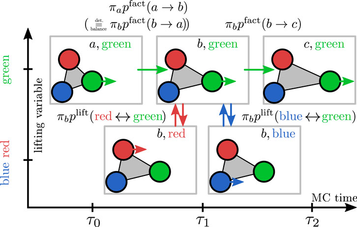
FIGURE 5. Conditional lifting in a system with three-particle interaction. The conditional lifting probabilities can be derived from the balance condition. Analogously to Figure 2 (i.e., using Eq. 5 and dividing by ${\pi }_b$) and decomposing the lifting probabilities according to Eq. 15 and choosing ${\lambda }_{\text{red}\to \text{green}}\equiv {\lambda }_{\text{green}}$, we get ${[-d{\mathrm{ℰ}}_{\text{green}}]}^{+}={\left[d{\mathrm{ℰ}}_{\text{red}}\right]}^{+}{\lambda }_{\text{green}}+{\left[d{\mathrm{ℰ}}_{\text{blue}}\right]}^{+}{\lambda }_{\text{green}}$ from the inflowing probability fluxes, leading to ${\lambda }_{\text{green}}={[-d{\mathrm{ℰ}}_{\text{green}}]}^{+}/\left({\left[d{\mathrm{ℰ}}_{\text{red}}\right]}^{+}+{\left[d{\mathrm{ℰ}}_{\text{blue}}\right]}^{+}\right)$. Note that this can be extended to match Eq. 20.

Inserting (15) this results in the condition

${\left[d{\mathrm{ℰ}}_{c_j\to b_j}\left(ijk\right)\right]}^{+}{\lambda }_{ji}+{\left[d{\mathrm{ℰ}}_{c_k\to b_k}\left(ijk\right)\right]}^{+}{\lambda }_{ki}={\left[-d{\mathrm{ℰ}}_{a_i\to b_i}\left(ijk\right)\right]}^{+}.(17)$

As for pairs, lifting from particle i to j will only take place (${\lambda }_{ij}>0$) if $d{\mathrm{ℰ}}_{a_i\to b_i}>0$ giving rise to a rejection of $a_i\to b_i$, and if the corresponding $d{\mathrm{ℰ}}_{c_j\to b_j}<0$ because of Eq. 17. Translational invariance of the interaction implies $d{\mathrm{ℰ}}_{a_i\to b_i}+d{\mathrm{ℰ}}_{c_k\to b_k}+d{\mathrm{ℰ}}_{c_j\to b_j}=0$. Writing out Eq. 17 analogously also for lifting to j and k, we can determine all conditional lifting probabilities uniquely [15],

${\lambda }_{ij}=\text{Θ}\left(d{\mathrm{ℰ}}_{a_i\to b_i}\right)\frac{{\left[-d{\mathrm{ℰ}}_{c_j\to b_j}\right]}^{+}}{{\left[d{\mathrm{ℰ}}_{a_i\to b_i}\right]}^{+}+{\left[d{\mathrm{ℰ}}_{c_k\to b_k}\right]}^{+}},(18)$

where $\text{Θ}\left(x\right)$ is the Heaviside step function.

For arbitrary $\mathcal{N}$, the global balance condition (17) generalizes to

${\displaystyle \sum }_{j\in M_{\mathrm{ℰ}}}{\left[d{\mathrm{ℰ}}_{c_j\to b_j}\right]}^{+}{\lambda }_{ji}={\left[-d{\mathrm{ℰ}}_{a_i\to b_i}\right]}^{+},(19)$

For $\mathcal{N}>3$, the choice of conditional lifting probabilities is not unique [15]. They can be fixed by the additional requirement ${\lambda }_{ji}\equiv {\lambda }_i$, that they are independent of the particle j we are lifting from as in (18). This leads to the simple general result

${\lambda }_{ij}=\text{Θ}\left(d{\mathrm{ℰ}}_{a_i\to b_i}\right)\frac{{\left[-d{\mathrm{ℰ}}_{c_j\to b_j}\right]}^{+}}{{\left[d{\mathrm{ℰ}}_{a_i\to b_i}\right]}^{+}+{{\displaystyle \sum }}_{k\in M_{\mathrm{ℰ}}\backslash \left\{i,j\right\}}{\left[d{\mathrm{ℰ}}_{c_k\to b_k}\right]}^{+}}.(20)$

Regardless of the number of interacting particles $\mathcal{N}$ in an interaction in $S_i$, the first step of calculating the rejection distance does not differ and is given by (13). For $\mathcal{N}=2$, the lifting destination when a rejection occurs is unambiguous, hence ${\lambda }_{ij}=1$. For $\mathcal{N}\ge 3$, the probability to lift from the active particle i to one of the other interacting particles $j\in M_{\mathrm{ℰ}}$ is also proportional to ${\lambda }_{ij}\propto {[-d{\mathrm{ℰ}}_j]}^{+}$ (see Eq. 20), which can be interpreted as the force which is exerted on the particle j by the interaction. Note that the conditional lifting probability vanishes when the particle, one would lift to, will increase the energy when moving along the current EC direction. We want to highlight that due to symmetry the sum of all forces must vanish ${\displaystyle \sum }_{j}d{E}_j=0$ and i can only trigger an event when $d{E}_i>0$ holds, which implies that for at least one other particle $d{E}_j<0$ must hold. In short, one most probably lifts to the particle, which decreases the interaction energy the fastest.

1.3.3 One-Particle Interactions

Finally, soft external one-particle potentials $\mathrm{ℰ}\left(i\right)$ frequently occur in soft matter systems, for example, as confining potentials, gravity, or external electric fields for charged particles. Such one-particle potentials are handled analogously to hard walls. Because there are no interaction partners the lifting variable is the EC direction $\mathbf{d}$. The lifting probability

$p_{\mathrm{ℰ}}^{\text{lift}}\left(\mathbf{d}\to d^{\prime }|a_i\to b_i\right)={\left[d{\mathrm{ℰ}}_{a_i\to b_i}\right]}^{+},(21)$

for lifting the EC direction to a reflected direction $d^{\prime }$ during an attempted move $a_i\to b_i$. The reflection can be performed with respect to the equipotential surface of $\mathrm{ℰ}\left(i\right)$, i.e., by lifting to $d^{\prime }=\left(1-2\mathit{P}\right)\mathbf{d}$, where $\mathit{P}$ is the projection operator onto the ${\nabla }_i\mathrm{ℰ}\left(i\right)$-direction. This has been shown to satisfy global balance [17].

1.4 ECMC Algorithm

In summary, an ECMC simulation, which we use for soft matter systems, can be structured as follows. Starting from a random particle i in a random EC direction $\mathbf{d}$ and with a certain EC total displacement $\ell$, the rejection distance $w_{ij}$ for each interaction $\mathrm{ℰ}\in S_i$ is calculated from Eq. 13 and as shown in Figure 4. The shortest distance determines which interaction caused the rejection. If the interaction consists of more than two particles, the conditional lifting probabilities ${\lambda }_{ij}$ are calculated from Eq. 20 and as illustrated in Figure 5. Then we lift to the corresponding interacting particle j after the corresponding rejection distance $w_{ij}$. For one-particle interactions causing the rejection we lift the EC direction by reflection.

1. choose a random EC direction $\mathbf{d}$, a total displacement $\ell$ and an active particle i,

2. calculate the minimal rejection distance $r_{M_{\mathrm{ℰ}}}={\text{min}}_{\mathrm{ℰ}\text{'}\in S_i}{w}_{i{M}_{\mathrm{ℰ}\text{'}}}$ for each $\mathrm{ℰ}$ according to Eq. 13,

3. if rejection is triggered by a three- or more particle interaction:select$j\in M_{\mathrm{ℰ}}$ by applying conditional lifting probabilities from Eqs (18) or (20) (see Figure 5),

4. move particle i: ${\mathbf{r}}_i={\mathbf{r}}_i+r\mathbf{d}$,

5. lift to rejecting particle $i\to j$ (or to new reflected EC direction $\mathbf{d}\text{'}$ if rejection is triggered by a one-particle interaction),

6. let$\ell =\ell -r$,

7. if$\ell =0$ goto 1 else goto 2

1.5 Additional ECMC Simulation Features

We want to highlight some useful properties of an ECMC simulation. First, using the factorized Metropolis filter each interaction is independent, making it easy to implement the algorithm in a highly modular manner.

Furthermore, the rejection distance distribution and lifting statistics is intimately linked to the pressure in the system. Without loss of generality, let the EC direction be in x-direction, then the pressure can be expressed by [13].

$\frac{P}{\rho k_{B}T}=\langle \frac{x_{\text{final}}-x_{\text{initial}}}{\ell }\rangle ,(22)$

where $\langle \dots \rangle$ denotes an ensemble average over multiple ECs with length $\ell$. Rewriting $x_{\text{final}}-x_{\text{initial}}=\ell +{\displaystyle \sum }_{\text{events}}\left(x_j-x_i\right)$, where $x_{i,j}$ are the x-coordinates of particles i and j, one sees that the excess length per EC length determines interaction specific contributions to the pressure of an ideal gas, i.e., attractive interactions with a negative excess length decrease the pressure, and repulsive interactions increase the pressure. This procedure does not need any additional computations. For hard spheres, the pressure is measured far more efficient than with the usual detour via the contact theorem.

Every configuration visited is weighted properly even if a hard sphere collision just happened. This can be exploited by special MC moves. This is not unconditionally true in a molecular dynamics simulation where, for instance, the statistics is skewed if measurements are taken on particle collisions. Inclusion of special many-particle MC moves can be beneficial for particular systems. For polymer melt simulations, we introduce a bead-swapping move [20], which switches positions of two hard spheres upon collision obeying a standard metropolis filter for the spring energies involved, as explained later.

Many simulation techniques based on single particle moves can benefit from massive parallelization if the simulation system can be efficiently divided into independent pieces. For ECMC algorithms, massive parallelization will not be optimal because of the cluster nature of EC moves [21]. In Ref. [21], a parallelization scheme for the EC algorithm was introduced, and extensive tests for correctness and efficiency were performed for the hard sphere system in two dimensions. For optimal parameters the algorithm achieves a speed up by a factor of roughly the number of cores used compared to a sequential EC simulation. For parallelization we use a spatial partitioning approach into simulation cells. We analyzed the performance gains for the parallel EC algorithm and find the criterion $\ell \sim L{\lambda }_0/\sqrt{n}\sigma$ for an optimal degree of parallelization, where n is the number of parallel threads, L the system size, and η the occupied area fraction. If the number n of parallel threads is chosen too large (massive parallelization), this choice for $\ell$ will drop below the optimal window $\ell <10{\lambda }_0$. Because massive parallelization is not optimal, the parallel EC algorithm will be best suited for commonly available multicore CPUs with shared memory. This ECMC parallelization scheme can also be applied to other soft matter systems such as polymer melts [20].

2 Applications

We now briefly present some soft matter systems where we successfully employed ECMC algorithms, namely a dense polymer melt, a network-forming system of polymers with a short range attraction, hard needle models of liquid crystal and liquid crystal colloids from a mixture of needles and hard spheres. In all of these systems the ECMC algorithm speeds up simulations considerably at high particle densities as compared to standard local MC simulations. The simulations for these soft matter applications have been performed within the highly modular polyeventchain framework, which is particularly suited for soft matter applications and will be presented in detail elsewhere. Jellyfish provides a similar EC framework with a focus on all atom simulations [22, 23].

2.1 Initialization and Simulation of Polymer Melts

The simulation of polymer melts by Molecular Dynamics (MD) or MC simulations is a challenging problem, in particular, for long chains at high densities, where polymers in the melt exhibit slow reptation and entanglement dynamics. For chain molecules of length N the disentanglement time increases $\propto N^3$ [24], which makes equilibration of long chain molecules in a melt a numerically challenging problem if only local displacement moves of polymer segments are employed as in a typical off-lattice MC simulation with fixed bond lengths [25–28] or fluctuating bond lengths [29], or in MD simulations [30–32], or for highly confined and therefore extremely packed melts [33]. In MD simulations, reptation dynamics has been successfully identified in the entangled regime [30–32, 34]. In MC simulation, reptation dynamics has been first identified in lattice models [35] or fluctuating bond lattice models [36] with Rouse-like local bond moves.

In MC simulations, non-local or collective MC moves can be introduced, for example, chain-topology changing double-bridging moves [37], which speed up equilibration; dynamic properties, however, are no longer realistic if such collective MC moves are employed. Likewise, reptation can also be introduced as explicit additional local MC reptation move [28, 38] (slithering snake moves) to obtain faster equilibration of a polymer melt but reptation dynamics is no longer dynamically realistic then.

In order to apply the above scheme of ECMC simulations to polymer melts, flexible polymers are modeled by a bead-spring model consisting of hard spheres, which are connected by harmonic springs [20]. These are the only additional soft pair interactions in the ECMC scheme for a flexible polymer melt. We choose the bond rest length to equal the hard-sphere diameter σ and a sufficiently large bond stiffness such that bond-crossing becomes inhibited by the impenetrable hard spheres and polymers remain entangled.

ECMC simulations can speed up MC simulations of polymers such that simulation speeds become comparable to MD simulation speeds and such that reptation dynamics can be clearly observed [20]. In each EC move, all beads that would collide successively during a short time interval in a MD simulation are displaced at once. This gives rise to a ECMC dynamics which is effectively very similar to the realistic MD dynamics and statements about polymer dynamics are still possible. In Ref. [20] we compared the ECMC algorithm to MD simulations implemented in LAMMPS regarding the equilibration of polymer melts. We utilized the time, that the positional fluctuation of the most inner bead of each polymer needs to reach the diffusive regime, as gauge to introduce an ad-hoc interpretation of time in the MC simulation (see Table I and Figure 5 in Ref. [20]). This showed that LAMMPS equilibrates more efficiently for moderate chain lengths. For long polymers ($N=500$) and when using an additional swap-move, ECMC simulations become equally performant, suggesting clear advantages for melts with even longer polymers.

The additional swap-move chanes the topology of entanglements locally. In contrast to the double-bridging move, which changes bonds, the swap move changes topology by changing bead positions. For this purpose we modify the EC move so that the EC does not directly transfer to the next bead upon hard sphere contact but, instead, a swap of the two touching spheres is proposed, see Figure 6. Such an additional swap move is EC specific and allows for a local change of entanglements. An analogous swap move in a standard MC algorithm needs to select pairs of beads such that the swap move has a reasonable acceptance rate (the particles have to be reasonably close). Moreover, the selection rule has to satisfy detailed balance (for example, simply proposing the nearest neighbor for swapping will lead to a violation of detailed balance). Therefore, there is no straightforward analogue of the EC swap move in a standard MC simulation with local moves.

FIGURE 6

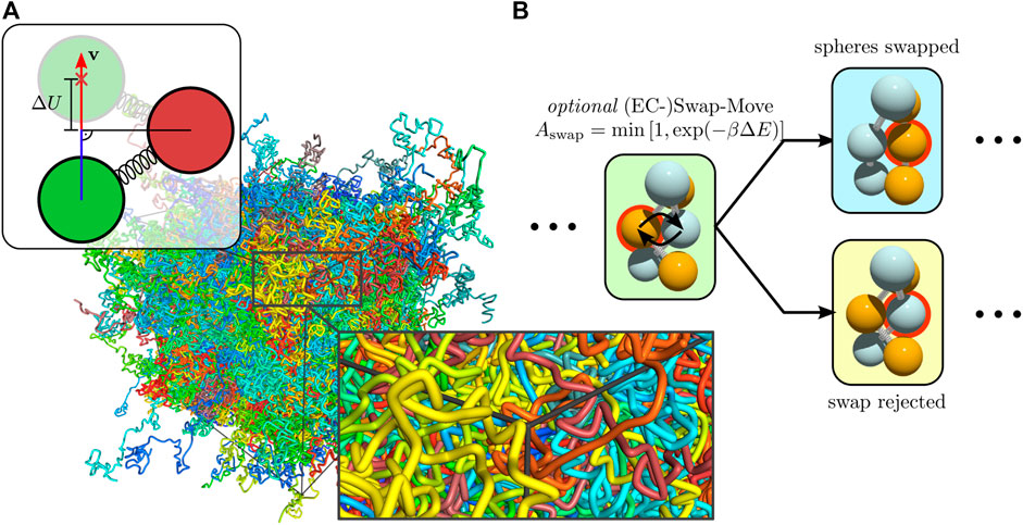
FIGURE 6. The background shows a polymer melt of flexible chains, which are presented as volumetric splines (A) Scheme for the rejection distance for hard sphere chains. If two bonded spheres do not collide, the active sphere can move freely until the minimal distance between both is reached. A usable energy $\text{Δ}E$ is drawn (see Figure 4) which determines where the rejection takes place (B) Scheme of a swap move. In case of a hard sphere collision, the energy difference of each involved springs is calculated when the beads would switch positions. The swap move is accepted with a standard Metropolis filter, otherwise the EC is continued normally. The active particle is marked by a red circle.

Here, we want to focus on another important aspect of EC moves in polymer melt simulations. EC moves can also be employed to generate initial configurations that are already representative of equilibrium configurations. This keeps the equilibration or warm-up phase of any subsequent simulation scheme (MC or MD) short. An early strategy to generate initial conditions is to slowly compress a very dilute equilibrated melt, which can take a long time for very dense target systems and becomes more difficult when chain lengths increase [30]. Another method that has been proposed first distributes the chains without interaction (phantom chains) and tries to resolve overlaps in a way which distorts the chain statistics as least as possible [30]. Over the years more sophisticated ways of resolving overlaps have been proposed, for instance a slowly increase of the strongly repulsive excluded volume potential [32]. This procedure is called push-off and the rate at which the potential is increased and the potential range is extended determines to a large extent how much the original statistics of the chains are disturbed. The method can also be applied to more realistic polymer models [39]. Recent work by Moreira et al. [40] shows how the procedure of Auhl et al. can be applied more efficiently and how the equilibration time can be shortened roughly by a factor of 6. An alternative strategy that performs even better for very long chains (again by a factor of $\sim 5$) has been introduced by Zhang et al. [41]. They employ a hierarchical approach, which uses sequential backmapping from a coarse-grained representation in order to re-introduce molecular details.

We present an EC-based scheme that is similar to the push-off scheme and takes advantage of the fact that the EC algorithm is well suited to resolve overlaps. To do this, ECs are started in random directions on any sphere that overlaps with at least one other sphere until all overlaps of this sphere are resolved. This procedure ignores spheres that overlap with the active sphere, so that the algorithm itself does not need to be changed. This procedure corresponds to locally rattling the polymer system, and can create enough space around the overlapping bead to insert it.

For relatively dense melts, Flory [44, 45] puts forward the hypothesis that the volume exclusion effect (chain swelling, $\langle R^2\rangle \sim N^{2\nu }$ with $\nu \ge 1/2$) is exactly compensated by the pressure generated by surrounding chains, so that a chain shows ideal behavior again. More recent results [42, 43] show that this hypothesis is only a good approximation. In particular, the tangent-tangent correlation of long ($N>500$) polymers in a melt falls algebraically, which deviates significantly from exponential decorrelation happening in the single polymer, i.e., free case.

This motivates the following scheme to generate pre-equilibrated polymer melts. Since excluded volume interactions between parts of a given chain are more or less screened as Flory suggests, we place phantom/ideal chains into the system in configurations that resemble non-reversal configurations by excluding a certain angular region for backward steps in generating the initial phantom chain configurations as described in Ref. [32]. This captures the structure of the chains on all length scales quite well, but comes with the downside that the asymptotic behavior of the end-to-end distance (the asymptotic Flory ratio $\langle R^2\rangle /\left(n\langle b^2\rangle \right)$) must be known beforehand to tune the excluded angular region accordingly. Luckily, the internal structure of the chains depends not strongly on the chain length and the asymptotic behavior can be determined in a faster system of shorter chains (here, we carried out one long run. Theoretical and numerical values for this ratio can be found in Ref. [46] and references therein).

The resulting phantom chain system is then equilibrated for a short time, so that the phantom chains will relax toward ideal chain configurations, i.e., the phantom chains contract starting from the initial non-reversal configurations. Then the hard sphere diameter is increased from $\sigma =0$ (phantom chains) to the target σ at once¹, which gives rise to overlaps. Then we use the EC rattling moves to resolve overlaps in the system. Switching on the hard sphere diameter will swell the chains and, therefore, have the opposite effect to the pre-equilibration. Both steps cancel each other well, resulting in high quality initial conditions. The quality can be assessed by comparison of equilibrium values of observables, such as $\langle R^2\rangle$, pair distribution $g\left(r\right)$, or bead distributions, with ensemble values given by the initial condition generation as shown in Figure 7.

FIGURE 7

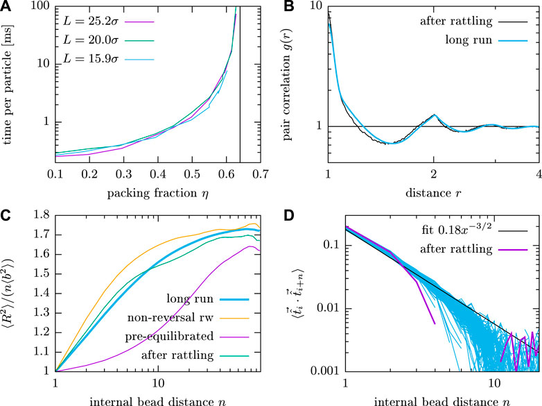
FIGURE 7. (A) Wall time per particle to generate rattled configurations of variable polymer number M with a fixed length of $N=200$. The wall time scales linearly in the numbers of particles, i.e., curves for different system sizes $L\times L$ are identical and diverge when the packing fraction $\eta =MN\left(\pi /6\right)\left({\sigma }^3/L^3\right)$ approaches the random closed packed limit ${\eta }_{rcp}\approx 0.64$ (indicated as vertical line). Preparation of even larger systems ($M\times N={10}^6$) for moderate η ($\approx 0.4$) take only $\approx {10}^3\text{s}$. Preparation of pure hard sphere systems ($N=1$) are roughly twice as fast. For the following we use $M=1000$ chains à $N=100$ beads at $\eta \approx 0.45$ ($\rho =0.85/{\sigma }^3$, i.e., $L\approx 49\sigma$). All data is generated on a single core of a i7-8650U (B) The pair correlation $g\left(r\right)$ is sensitive to the local structure of the hard spheres and resembles the equilibrium measurement quite well. The warm-up takes only a couple of minutes (C) The internal bead-to-bead distance $\langle R^2\rangle /\left(n\langle b^2\rangle \right)$ captures how well the polymers are equilibrated and has to be as close to the equilibrium result as possible because this observable equilibrates very slowly. For equilibration a chain needs to move its own size, which is slow due to reptational dynamics. Because of strong fluctuations the warm-up times have not been measured precisely, but are of the order of a couple of hours (D) The tangent correlation shows the correct non-ideal behavior of chains in the melt [42, 43]. The configuration after rattling resembles the equilibrium quite well. The warm-up takes only a couple of minutes.

For this procedure it is vital that the spring constant is quite large. Starting ECs on one particle until overlaps are resolved obviously breaks balance. Presumably, setting the spring constant to a relatively high value (in Figure 7$k=\mathrm{1,000}{k}_{B}T/{\sigma }^2$, where the rest length is identical to the hard sphere diameter $b_0=\sigma$) leads to less distortions along the chain.

In general, it is hard to quantitatively compare time scales and thus performance of the EC-based initialization scheme with other schemes from the literature. Hardware development over the years (Moore’s law, number of cores, etc.), underlying polymer models (volume exclusion: hard spheres vs. Lennard-Jones, bonding: harmonic springs vs. FENE vs. tangent hard spheres vs. united atom force fields), criteria of deciding when equilibrium is reached, or simply untested parameter dependencies (regarding system size, chain length, spring constants) can have non-trivial influence, even on an otherwise robust benchmark. Despite these problems to compare quantitatively, the proposed EC-based method seems comparable to other state-of-the-art methods. This has to be checked further in future work.

2.2 Self-Assembly of Filament Bundle Networks

The cytoskeleton is a mechanically important structure which consists of three classes of interacting filamentous proteins (microtubules, filamentous F-actin, intermediate filaments) in animal cells. The different constituents reflect the multi-functionality of the cytoskeleton and the different requirements with respect to force and time scales. F-actin structures in the cell cortex are most important for cell mechanics and cell motility [47, 48]. From the polymer physics point of view, F-actin is a semiflexible polymer since typical contours lengths are of the same order as its persistence length. Therefore, bending rigidity and thermal fluctuations are relevant to understand F-actin structures. Within the cell, F-actin forms locally very dense sub-cellular structures like bundles [49], networks and even networks of bundles to fulfill their biological functionality [47]. In vivo, bundles and also networks are held together by crosslinking proteins [50].

Also minimal cytoskeletal in vitro systems [50], some of which are confined to droplets [51, 52] or in microfluidic chambers [53–55], show formation of bundles and also networks of bundles under the influence of attractive interactions. In vitro, such attractive interactions can not only be induced by crosslinkers but also by counterions and depletion interactions.

The simulation of the cytoskeleton of a cell is a long-standing problem as its physical properties are often governed by the interplay of many long polymers, which are deformable by thermal fluctuations against their bending rigidity and subject to crosslinker-mediated attractive interactions [56]. Theoretical work on crosslinker-mediated bundling of semiflexible polymers [56–59] and the related problem of counterion-mediated binding of semiflexible polyelectrolytes [60] show a discontinuous bundling transition above a threshold concentration of crosslinkers or counterions. The nature of the crosslinkers can influence the mechanical properties of polymer bundles [61].

Simulations of few filaments clearly confirm bundling in a single transition [56]. The emerging bundles of semiflexible polymers (Figure 8) are typically rather densely packed which causes difficulties in equilibrating bundled structures in traditional MC simulations employing local moves. In Ref. [56], MC simulations showed evidence for kinetically arrested states with segregated sub-bundles; in Ref. [62], kinetically arrested bundle networks have been observed for rather small semiflexible polyelectrolyte systems. Further numerical progress requires a faster equilibration of dense bundle structures. Simulations of larger systems consisting of cytoskeletal filaments and crosslinkers [63–65] show different competing phases from isotropic networks to bundles and other aggregates, for example, with bond-orientational order. In Ref. [65], it was also pointed out that the dynamics of bundling and polymerization in combination with entanglement of polymers strongly influence the resulting structure. This raises the question to what extent bundled structures can reach a genuine equilibrium under realistic conditions.

FIGURE 8

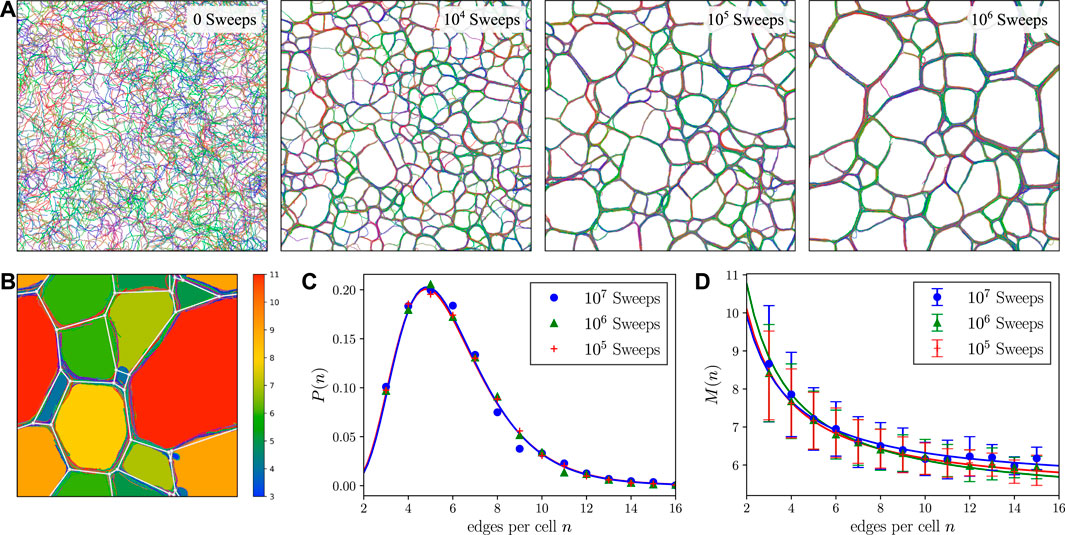
FIGURE 8. (A) A series of snapshots (after 0, ${10}^4$, ${10}^5$, ${10}^6$ sweeps; in a sweep, each sphere is moved once on average); demonstrating coarsening. The snapshots are taken from a simulation of $M=1000$ polymers à $N=100$ beads in a $400\sigma \times 400\sigma \times 10\sigma$ simulation box. The simulation is performed with the following parameters: bending constant $\kappa =30k_{B}T\sigma$, spring constant $k=100k_{B}T/{\sigma }^2$ and rest length $b_0=\sigma$, potential strength $g=0.7k_{B}T$ and range $d=0.4\sigma$. A random color is assigned to each polymer for clarity (B) Example of a simple graph representation (white balls and bonds) as overlay over a network snapshot generated by an automated procedure to identify vertices (white balls) and edges (white bonds) of the bundle network. The color of cells codes for the number of enclosing edges. All data in Figs. C and D is measured from such graphs. For clarity, we use a comparatively small system (C) Distribution $P\left(n\right)$ of the number of edges n per cell for different simulation times. The curves are obtained by fitting log-normal distributions to the data (D) Aboav-Weaire law $M\left(n\right)$ for different simulation times, which measures the mean edge counts of neighboring cells. Cells with a high number of edges tend to have neighboring cells with fewer edges and vice versa. Error bars represent one standard deviation. The Aboav-Weaire law, the fits of $P\left(n\right)$ in C as well as direct computation of the variance ${\mu }_2$ of the number of edges per cell yield similar values ${\mu }_2\sim 5.2$ for the simulation parameters given in A.

Further numerical progress requires a faster equilibration of dense bundle structures, for which the ECMC algorithm is ideally suited [21]. In comparison to polymer melts, two additional interactions have to be included in this system: (i) Polymers are semiflexible such that we have to include a bending rigidity of each bead-spring polymer, which is an example of a three-particle interaction between three neighboring hard sphere beads along a polymer. (ii) There is a short-range attraction, which mimics a crosslinker- or counterion-mediated attraction between polymers. Therefore, all beads also interact pairwise with a short-ranged attractive square well potential of strength g and range d. We choose a potential strength g well above the critical value for bundling [56, 59], and the range of the attractive square well potential is $d=0.4\sigma$, i.e., comparable to the filament radius (bead radius). Both additional interaction energies are incorporated in the ECMC polymer simulation. Again, it is important to note that we expect a qualitatively realistic MC dynamics from ECs, which resembles collisions in MD simulations. The performance can be further increases by parallelization as discussed above [21].

We have applied this ECMC algorithm to a system consisting of many² interacting semiflexible polymers, such as actin filaments, in a flat simulation box in three dimensions. Periodic boundary conditions are used only for the extended direction of the simulation box whereas the spatially short direction is non-periodic. Under the influence of the short-range attraction, we clearly observe formation of densely packed bundles. We also observe that, starting from an isotropic melt-like situation, it is not a single bundle that forms but the system evolves into a structure consisting of a network of bundles.

The simulation does not reach a truly equilibrated stationary state, but the network of bundles keeps evolving by coarsening processes as shown in Figure 8A. This clearly demonstrates that the assembly dynamics plays an important role in structure formation in these systems, as similarly suggested in Ref. [65]. As mentioned above, the ECMC dynamics is effectively very similar to the realistic MD dynamics. Therefore, the observed coarsening dynamics is not an artifact of the MC simulation but a generic property of this multi-filament system. On the time scales of our simulations (up to ${10}^7$ MC sweeps) the bundle system keeps evolving by coarsening and no genuine equilibrium state is reached.

Our preliminary results suggest that the bundle networks form structures similar to foams [66], which also continue to coarsen over time, see Figure 8. The dynamics of the coarsening process exhibits further analogies. It can be observed that cells in the bundle network, which enclose a comparatively large area, tend to increase their area at the expense of cells with smaller enclosed area. This behavior is known from foams as a consequence of the von Neumann law for the area growth rate of cells [67] and of the correlation between relative bubble volume and the number of sides [68]. However, the von Neumann law assumes an exchange of the enclosed medium by diffusion through the liquid interfaces and cannot be applied directly to the bundle networks considered here. Other empirical laws found in the context of foams like Aboav-Weaire law [69] for the mean number $M\left(n\right)$ of sides of cells surrounding an n-sided cell can also be applied very well to the emerging bundle networks (see Figure 8D). The Aboav-Weaire law is of particular interest since it provides an alternative approach to determine the variance ${\mu }_2$ of the mean number of edges per cell (denoted as $P\left(n\right)$ in Figure 8C). Comparison of the value of ${\mu }_2$ computed directly from the data to the values obtained from fit parameters of $P\left(n\right)$ and the Aboav-Weaire law yields a reasonable agreement.

While the structure formation in dry foams is driven by the minimization of interfacial energies and diffusion [70], it appears that the bundle networks coarsen by a zipping mechanism [71, 72] which leads – similar to the decrease in interfacial energy in foams – to a decrease of the polymer binding energy (i.e., to more adhesive contacts between polymers). At a fixed amount of polymers this gives rise to a minimization of bundle length, which plays an analogous role to the minimization of surface area in a classical three-dimensional foam. The foam-like bundle networks resemble the structures observed in different in vitro experiments [51, 53], where also polygonal cell structures of the self-assembled networks have been observed.

2.3 Liquid Crystals and Colloidal Suspensions

Composite soft matter systems such as colloidal mixtures containing different colloidal particles, often of different size, represent challenging systems for simulations because their physics are typically governed by effective interactions which arise if microscopic degrees of freedom of one species are integrated out. Effective interactions are essential to characterize stability and potential self-assembly into crystalline phases but hard to access in a microscopic particle-based simulation. The process of integrating out microscopic degrees of freedom corresponds to the numerical evaluation of a potential of mean force between the colloidal species of interest. In order to measure the potential of mean force for one colloidal species accurately, all degrees of freedom must be properly equilibrated.

As an example of such a colloidal mixture we consider a two-dimensional system of needles and colloidal disks. This serves as a simple model system for liquid crystal (LC) colloids, which are colloidal particles suspended in a liquid crystal. Such LC colloids exhibit anisotropic effective interactions between colloidal particles if the LC is in an ordered, e.g., nematic phase [73, 74]. A nematic LC phase forms a rich variety of defect-structures around a spherical inclusion such as Saturn-ring disclination rings or a satellite hedgehog for normal anchoring and boojums for planar anchoring [75–77]. In a dense nematic LC, the effective interactions can be governed both by depletion interactions [78] or by long-range elastic interactions mediated by director field distortions in the nematic hard needles. Because hard needles tend to align tangentially at a hard wall, we expect a quadrupolar elastic interaction, which is characteristic for planar anchoring at the colloidal disk [79–83] but also generic in two dimensions [84]. This interplay has been studied in Ref. [85] employing an ECMC simulation.

The colloidal mixture of hard disks suspended in a nematic host of hard needles is particularly challenging as the hard needle system must be fairly dense to establish a nematic phase. While particle-based simulations exist for dilute rods in the isotropic phase [86, 87], the regime of a nematic host is fairly unexplored up to now and simulations resorted to coarse-graining approaches [83]. So far, only single inclusions [88] or confining geometries [89] have been investigated by particle-based simulations. In order to measure the potential of mean force for larger colloidal disks accurately, all degrees of freedom of the needles but also the relatively slow degrees of freedom of the colloidal disks must be properly equilibrated. This is efficiently achieved by the ECMC algorithm.

The idea for the ECMC simulation of a needle system is to represent needles by their two endpoints, where only one endpoint is moving at a time [15]; the endpoints are connected by an infinitely thin, hard line. For efficient sampling, the distance of the two endpoints, i.e. the length l of the hard needle can fluctuate around its characteristic length $l_0$ in order to allow for independent motion of both endpoints in the MC simulation; the needle length l is restricted by a tethering potential $V_{\text{n}}\left(l\right)$ with $V_{\text{n}}\left(l\right)=0$ for $l/l_0\in [0.9,1.1]$ and infinite $V_{\text{n}}\left(l\right)$ else, such that $l_0$ is the effective needle length. This constitutes an additional pair potential in the ECMC framework.

In two dimensions, the needle-needle interaction simplifies effectively to a collision of an endpoint with another needle. The remaining MC move distance is lifted to one of the endpoints of this needle. Therefore, we have a fluid of endpoints with an effective three-particle interaction (two endpoints of a passive needle and the active endpoint). For needles the probability ${\lambda }_{ij}$ to which endpoint is lifted (see Eq. 20) is simply proportional to the distance to the other endpoint, i.e., it is lifted with higher probability to the closer endpoint.

In a composite colloidal problem the ECMC algorithm also faces the problem of lifting between different species. This can be performed exactly according to the same rules as lifting between a single species. In the presence of additional disks, MC displacement of needle endpoints is also lifted to disks if a needle collides with the disk and vice versa as illustrated in Figure 9A. The example of a needle system also shows that collision detection is often the computational bottleneck of ECMC simulations. Here, we use a sophisticated neighbor list system to achieve high simulation speeds also in the nematic phase. Each particle is confined to a container, which triggers an event when the particle leaves it. Then the neighbor list is updated, which ensures that the neighbor lists are always valid. Particles are added to the neighbor lists of the other particle and vice versa when their containers overlap. This way, for different particles different container shapes can be chosen. For the needles, a very narrow rectangle can be used, which limits the computational effort for calculating the distances to the next collision and makes the simulation significantly more efficient in the nematic phase. In particular, the anisotropy of the needles can be assigned particularly well without sacrificing any flexibility for the bookkeeping of the spheres. Furthermore, we optimize the updating of lists by putting them onto a collision grid.

FIGURE 9

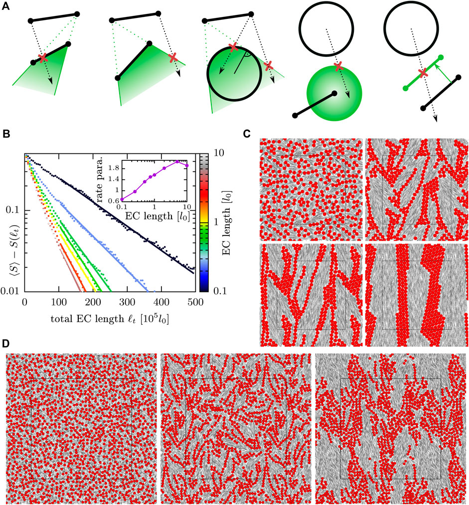
FIGURE 9. (A) List of all geometrical cases where rejections/lifting between needles and disks occur (first two depict needle-needle, the third needle-disk, and the last two ones sphere-needle collisions). If a needle is not hit at one of its endpoints (first and last picture) conditional lifting probabilities ${\lambda }_{ij}$ for a three-particle interaction are applied (B) Efficiency gains with increasing EC length $\ell$ for a two-dimensional needle system in a volume of $L\times L$ at density ${\rho }_{\text{n}}=10/l_0^2$. Starting at one random configuration an ensemble of simulations with different EC lengths are conducted. We show the difference between the nematic order parameter over time and the equilibrium value yielding an exponential. The decay rate of the order parameter is used as efficiency measure, where a simulation with $\ell =5l_0$ is 2.8 times more efficient than a simulation with $\ell =0.1$, where the latter took even 1.7 times the wall time, yielding a speed-up of $\approx 5$ between $\ell =0.1$ and $\ell =5=L/2$(C and D) Evolution of a mixture of hard needles of length ${ł}_0=1$ and hard disks with a diameter $\sigma =l_0$ indicating an effective interaction between disks, which favors parallel chaining (C) A system of size $20{ł}_0\times 20{ł}_0$ containing needles at density ${\rho }_{\text{n}}=20/l_0^2$ and 160 disks of diameter $\sigma =l_0$(D) a larger system of $40{ł}_0\times 40{ł}_0$ containing needles at density ${\rho }_{\text{n}}=10/l_0^2$ and 640 disks of diameter $\sigma =l_0$.

In Figure 9B, we show a detailed benchmarking for a two-dimensional pure needle system. With increasing EC length $\ell$, the sampling efficiency is increased, where an EC length comparable to the mean free path can be seen as the limit of a local MC simulation. In Figure 9B, we relax an isotropic initial configuration toward nematic equilibrium in a quite dense needle system at density ${\rho }_{\text{n}}=10/l_0^2$. The resulting relaxation of the nematic order parameter is exponentially, where we use the decay constant of the exponential as efficiency measure. For EC lengths approaching the system size, no further improvements occur as naively expected.

In three dimensions, hard needles introduce no excluded volume and therefore lack any phase transitions (we have checked with ECMC simulations not shown here that, independent of the density, the nematic order parameter vanishes for hard needles in equilibrium). In three dimensions hard spherocylinders are a natural extension of needles that introduces a non-vanishing excluded volume. As an additional proof of concept of our ECMC implementation with three-particle lifting, we investigate the series of liquid crystal phase transitions by monitoring the pressure as a function of increasing volume fraction, see Figure 10. We see a sequence of transitions from isotropic to nematic ordering, followed by a transition to smectic order, and ultimately, crystallization in complete agreement with literature results [90].

FIGURE 10

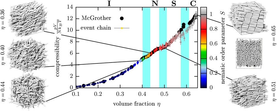
FIGURE 10. Phase diagram of hard spherocylinders (with diameter D and length $L=5D$) in three dimensions. We see four phases ($\mathbf{I}$—isotropic, $\mathbf{N}$—nematic, $\mathbf{S}$—smectic, $\mathbf{C}$—crystalline), in agreement with previous results by McGrother et al. [90] We added six snapshots at different volume fractions η to illustrate the different phases and phase transitions (also indicated by the blue regions).

For the colloidal mixture of hard disks suspended in a nematic host of hard needles, the ECMC simulation reveals a surprising and robust tendency for parallel chaining of disks along the director axis which seems to contradict the chaining in a ${45}^{\circ }$ angle with respect to the director axis as predicted by quadrupolar elastic interactions in two dimensions [82]. This is a result of a dominant short-range depletion interaction, which strongly favors parallel chaining [85]. The effective disk-disk interaction can be obtained as a potential of mean force by simulations of systems containing only two colloidal disks and is in good agreement with analytical calculations, where we add the depletion interaction mediated by needles on short scales and the elastic quadrupolar interaction mediated by a nematic needle LC which has weak planar anchoring at the colloidal disks and exhibits elastic anisotropy. Here, we demonstrate the validity of this results on a larger scale for systems containing many colloidal disks. Figures 9C,D show the equilibration process of 160 and 640 disks with diameter $\sigma =1$ in needle densities of ${\rho }_{\text{n}}=20/l_0^2$ and $10/l_0^2$, respectively, where $l_0$ is the equilibrium length of a needle. We clearly see that parallel chaining always corresponds to the equilibrium state of the composite system.

3 Discussion

We presented several applications that demonstrate how ECMC is an effective and fast simulation technique that is particularly suited for dense soft matter systems. Polymer melts, bundles of semiflexible polymers, and the composite system of a liquid crystal colloid are computationally challenging problems, where the ECMC techniques give an improved performance.

We started with an introduction to the algorithm, where we showed how arbitrary interactions between hard spheres can be easily included into the ECMC framework such that a multitude of soft matter systems can be modeled. On this algorithmic side, long-range interactions have not been covered explicitly here but can also be included in an effective manner [91].

Future developments will also address variations of the basic EC moves presented here in order to sample even more efficiently. On a generic collision, one interaction rejects the move and lifting occurs which means the current EC direction has a component parallel to the energy gradient of this specific interaction. One can resample the perpendicular parts of the EC direction in order to avoid reshuffling the EC direction from time to time, i.e., a finite EC length. This procedure has been recently developed and is called forward EC [92]. In specialized settings, the scheme seems very promising with regard to efficient sampling and should also be tested in the context of soft matter systems in the future.

On the application side in the soft matter field, we presented new results for the initialization and pre-equilibration of polymer melts, where a novel rattling algorithm based on ECs can be employed to efficiently remove overlaps in initial configurations. For large systems of semiflexible polymers with a short-range attraction, we demonstrated that ECMC simulations are capable to follow the formation of large networks of bundles and their subsequent foam-like coarsening behavior, see Figure 8. For a two-dimensional hard disk and needle model for LC colloids, the structure formation by parallel chaining of disks could be followed for large systems over large time scales as shown in Figure 9. Here we find that increasing the EC length, i.e., increasing the cluster size in our EC algorithm gives rise to considerable performance gains.

In summary, we addressed compact quasi-zero-dimensional hard sphere particles, one-dimensional hard rods or hard needles, and one-dimensional polymers as constituents in soft matter ECMC simulations. A natural extension for future work is the development of ECMC algorithms for two-dimensional triangulated surfaces with local elastic properties, which are impenetrable for other simulation objects, e.g., hard spheres or polymers. This will allow us to study fluctuating triangulated elastic membranes and, in a compound polymer-membrane system, polymer networks confined to elastic capsules. It was shown that the boundary conditions significantly contribute to the network structure [53]. The elastic properties of a triangulated surface can be described by a set of elastic energies such as the TRBS model [93], where elastic constants like Young’s modulus and Poisson ratio are adjustable and also bending stiffness can be included [94].

The actual implementation will be a very challenging problem. The interaction of a triangle with a point or a hard sphere is an effective 4-particle interaction. The rejection distance is efficiently calculable by the Möller “Trumbore intersection algorithm. To implement non-intersecting surfaces, interactions between two triangles have to be introduced, which can lead to a 6-particle interaction. Therefore, membrane simulations would also represent a further test of the general framework for $\mathcal{N}$-particle interactions in the EC algorithm [15]. The conditional lifting probabilities will look similar to the case of hard needles.

Based on the extensive experiences with EC based simulations presented here, we think this simulation technique is suitable to tackle large (biological) systems. In order to verify and evaluate the EC algorithm for triangulated surfaces, we can investigate the crumpling transition [95]. In Ref. [96], the necessary biophysical conditions for the formation of tubular membrane protrusions have been investigated and, it has been suggested that actin filaments polymerizing against a soft membrane are sufficient to form protrusions, which seems a suitable next system to explore the possibilties of EC algorithms for dense soft matter systems.

Data Availability Statement

The raw data supporting the conclusions of this article will be made available by the authors, without undue reservation.

Author Contributions

TAK conceived research, performed simulations, evaluated data, wrote and revised manuscript, acquired research funding; DM, LPW, CFV performed simulations, evaluated data; JK conceived research, wrote and revised manuscript.

Funding

TAK received support by the Deutsche Forschungsgemeinschaft (DFG) (Grant No. KA 4897/1–1).

Conflict of Interest

The authors declare that the research was conducted in the absence of any commercial or financial relationships that could be construed as a potential conflict of interest.

Footnotes

¹In our previous work [21] we suggested a steady increase of the hard sphere diameter (similar to the slow push-off) rather than introducing the full diameter at once, but actually implemented the procedure outlined here because of an implementation error. Therefore, the procedure in Ref. [21] was described wrongly, but still produced overlap-free, high quality initial conditions.

²We tried as many as $M=5000$ polymers à $N=200$ beads [20]. Since the system should be large enough when the typical cell scale is much smaller than the system size, we use smaller systems to improve the statistics and to get to coarsening.

References

1. Metropolis N, Rosenbluth AW, Rosenbluth MN, Teller AH, Teller E Equation of state calculations by fast computing machines. J Chem Phys (1953) 21:1087–92. doi:10.1063/1.1699114

CrossRef Full Text | Google Scholar

2. Hastings WK Monte Carlo sampling methods using Markov chains and their applications. Biometrika (1970) 57:97–109. doi:10.1093/biomet/57.1.97

CrossRef Full Text | Google Scholar

3. Swendsen RH, Wang J Nonuniversal critical dynamics in Monte Carlo simulations. Phys Rev Lett (1987) 58:86–8. doi:10.1103/PhysRevLett.58.86

PubMed Abstract | CrossRef Full Text | Google Scholar

4. Wolff U Collective Monte Carlo updating for spin systems. Phys Rev Lett (1989) 62:361–4. doi:10.1103/PhysRevLett.62.361

PubMed Abstract | CrossRef Full Text | Google Scholar

5. Bernard EP, Krauth W, Wilson DB Event-chain Monte Carlo algorithms for hard-sphere systems. Phys Rev E (2009) 80:056704. doi:10.1103/PhysRevE.80.056704

CrossRef Full Text | Google Scholar

6. Strandburg K Two-dimensional melting. Rev Mod Phys (1988) 60:161–207. doi:10.1103/RevModPhys.60.161

CrossRef Full Text | Google Scholar

7. Kosterlitz JM, Thouless DJ Ordering, metastability and phase transitions in two-dimensional systems. J Phys C (1973) 6:1181–203. doi:10.1088/0022-3719/6/7/010

CrossRef Full Text | Google Scholar

8. Halperin BI, Nelson DR Theory of two-dimensional melting. Phys Rev Lett (1978) 41:121–4. doi:10.1103/PhysRevLett.41.121

CrossRef Full Text | Google Scholar

9. Young AP Melting and the vector Coulomb gas in two dimensions. Phys Rev B (1979) 19:1855–66. doi:10.1103/PhysRevB.19.1855

CrossRef Full Text | Google Scholar

10. Mak CH Large-scale simulations of the two-dimensional melting of hard disks. Phys Rev E (2006) 73:065104. doi:10.1103/PhysRevE.73.065104

CrossRef Full Text | Google Scholar

11. Bernard EP, Krauth W Two-step melting in two dimensions: first-order liquid-hexatic transition. Phys Rev Lett (2011) 107:155704. doi:10.1103/PhysRevLett.107.155704

PubMed Abstract | CrossRef Full Text | Google Scholar

12. Engel M, Anderson JA, Glotzer SC, Isobe M, Bernard EP, Krauth W Hard-disk equation of state: first-order liquid-hexatic transition in two dimensions with three simulation methods. Phys Rev E (2013) 87:042134. doi:10.1103/PhysRevE.87.042134

CrossRef Full Text | Google Scholar

13. Michel M, Kapfer SC, Krauth W Generalized event-chain Monte Carlo: constructing rejection-free global-balance algorithms from infinitesimal steps. J Chem Phys (2014) 140:054116. doi:10.1063/1.4863991

PubMed Abstract | CrossRef Full Text | Google Scholar

14. Michel M, Mayer J, Krauth W Event-chain Monte Carlo for classical continuous spin models. EPL (Europhysics Lett (2015) 112. 20003. doi:10.1209/0295-5075/112/20003

CrossRef Full Text | Google Scholar

15. Harland J, Michel M, Kampmann TA, Kierfeld J Event-chain Monte Carlo algorithms for three- and many-particle interactions. EPL (Europhysics Letters) (2017) 117:30001. doi:10.1209/0295-5075/117/30001

CrossRef Full Text | Google Scholar

16. Diaconis P, Holmes S, Neal RM Analysis of a nonreversible Markov chain sampler. Ann Appl Probab (2000) 10:726–52. doi:10.1214/aoap/1019487508

CrossRef Full Text | Google Scholar

17. Peters EAJF, de With G Rejection-free Monte Carlo sampling for general potentials. Phys Rev E (2012) 85:026703. doi:10.1103/PhysRevE.85.026703

CrossRef Full Text | Google Scholar

18. Nishikawa Y, Michel M, Krauth W, Hukushima K Event-chain algorithm for the Heisenberg model. Phys Rev E (2015) 92:63306. doi:10.1103/PhysRevE.92.063306

CrossRef Full Text | Google Scholar

19. Gillespie DT Stochastic simulation of chemical kinetics. Annu Rev Phys Chem (2007) 58:35–55. doi:10.1146/annurev.physchem.58.032806.104637

PubMed Abstract | CrossRef Full Text | Google Scholar

20. Kampmann TA, Boltz HH, Kierfeld J Monte Carlo simulation of dense polymer melts using event chain algorithms. J Chem Phys (2015) 143:044105. doi:10.1063/1.4927084

PubMed Abstract | CrossRef Full Text | Google Scholar

21. Kampmann TA, Boltz HH, Kierfeld J Parallelized event chain algorithm for dense hard sphere and polymer systems. J Comput Phys (2015) 281:864–75. doi:10.1016/j.jcp.2014.10.059

CrossRef Full Text | Google Scholar

22. Faulkner MF, Qin L, Maggs AC, Krauth W All-atom computations with irreversible Markov chains. J Chem Phys (2018) 149:064113. doi:10.1063/1.5036638

PubMed Abstract | CrossRef Full Text | Google Scholar

23. Höllmer P, Qin L, Faulkner MF, Maggs A, Krauth W JeLLyFysh-Version1.0 — a Python application for all-atom event-chain Monte Carlo. Comput Phys Commun (2020) 253:107168. doi:10.1016/j.cpc.2020.107168

CrossRef Full Text | Google Scholar

24. Doi MSFE. The theory of polymer dynamics. London: Clarendon Press (1986).

25. Curro JG Computer simulation of multiple chain systems—the effect of density on the average chain dimensions. J Chem Phys (1974) 61:1203–7. doi:10.1063/1.1681994

CrossRef Full Text | Google Scholar

26. Baumgärtner A, Binder K Dynamics of entangled polymer melts: a computer simulation. J Chem Phys (1981) 75:2994–3005. doi:10.1063/1.442391

CrossRef Full Text | Google Scholar

27. Khalatur P, Pletneva SG, Papulov Y Monte Carlo simulation of multiple chain systems: the concentration dependence of osmotic pressure in two- and three-dimensional spaces. Chem Phys (1984) 83:97–104. doi:10.1016/0301-0104(84)85224-6

CrossRef Full Text | Google Scholar

28. Haslam AJ, Jackson G, McLeish TCB An investigation of the shape and crossover scaling of flexible tangent hard-sphere polymer chains by Monte Carlo simulation. J Chem Phys (1999) 111:416–28. doi:10.1063/1.479292

CrossRef Full Text | Google Scholar

29. Rosche M, Winkler RG, Reineker P, Schulz M Topologically induced glass transition in dense polymer systems. J Chem Phys (2000) 112:3051–62. doi:10.1063/1.480880

CrossRef Full Text | Google Scholar

30. Kremer K, Grest GS Dynamics of entangled linear polymer melts: a molecular—dynamics simulation. J Chem Phys (1990) 92:5057–86. doi:10.1063/1.458541

CrossRef Full Text | Google Scholar

31. Pütz M, Kremer K, Grest GS What is the entanglement length in a polymer melt?. Europhys Lett (2000) 49:735–41. doi:10.1209/epl/i2000-00212-8

CrossRef Full Text | Google Scholar

32. Auhl R, Everaers R, Grest GS, Kremer K, Plimpton SJ Equilibration of long chain polymer melts in computer simulations. J Chem Phys (2003) 119:12718–28. doi:10.1063/1.1628670

CrossRef Full Text | Google Scholar

33. Ramos PM, Karayiannis NC, Laso M Off-lattice simulation algorithms for athermal chain molecules under extreme confinement. J Comput Phys (2018) 375:918–34. doi:10.1016/j.jcp.2018.08.052

CrossRef Full Text | Google Scholar

34. Hsu HP, Kremer K Static and dynamic properties of large polymer melts in equilibrium. J Chem Phys (2016) 144:154907. doi:10.1063/1.4946033

PubMed Abstract | CrossRef Full Text | Google Scholar

35. Kremer K Statics and dynamics of polymeric melts: a numerical analysis. Macromolecules (1983) 16:1632–8. doi:10.1021/ma00244a015

CrossRef Full Text | Google Scholar

36. Paul W, Binder K, Heermann DW, Kremer K Dynamics of polymer solutions and melts. Reptation predictions and scaling of relaxation times. J Chem Phys (1991) 95:7726–40. doi:10.1063/1.461346

CrossRef Full Text | Google Scholar

37. Karayiannis NC, Mavrantzas VG, Theodorou DN A novel Monte Carlo scheme for the rapid equilibration of atomistic model polymer systems of precisely defined molecular architecture. Phys Rev Lett (2002) 88:105503. doi:10.1103/PhysRevLett.88.105503

PubMed Abstract | CrossRef Full Text | Google Scholar

38. Wall FT, Mandel F Macromolecular dimensions obtained by an efficient Monte Carlo method without sample attrition. J Chem Phys (1975) 63:4592–5. doi:10.1063/1.431268

CrossRef Full Text | Google Scholar

39. Sliozberg YR, Kröger M, Chantawansri TL Fast equilibration protocol for million atom systems of highly entangled linear polyethylene chains. J Chem Phys (2016) 144:154901. doi:10.1063/1.4946802

PubMed Abstract | CrossRef Full Text | Google Scholar

40. Moreira LA, Zhang G, Müller F, Stuehn T, Kremer K Direct equilibration and characterization of polymer melts for computer simulations. Macromol Theor Simulations (2015) 24:419–31. doi:10.1002/mats.201500013

CrossRef Full Text | Google Scholar

41. Zhang G, Moreira LA, Stuehn T, Daoulas KC, Kremer K Equilibration of high molecular weight polymer melts: a hierarchical strategy. ACS Macro Lett (2014) 3:198–203. doi:10.1021/mz5000015

CrossRef Full Text | Google Scholar

42. Wittmer JP, Beckrich P, Meyer H, Cavallo A, Johner A, Baschnagel J Intramolecular long-range correlations in polymer melts: the segmental size distribution and its moments. Phys Rev E (2007) 76:011803. doi:10.1103/PhysRevE.76.011803

CrossRef Full Text | Google Scholar

43. Wittmer JP, Beckrich P, Johner A, Semenov AN, Obukhov SP, Meyer H, et al. Why polymer chains in a melt are not random walks. Europhys Lett (2007) 77:56003. doi:10.1209/0295-5075/77/56003

CrossRef Full Text | Google Scholar

44. Flory PJ The configuration of real polymer chains. J Chem Phys (1951) 19:1315–6. doi:10.1063/1.1748031

CrossRef Full Text | Google Scholar

45. Flory PJ. Statistical mechanics of chain molecules. Oxford: Oxford University Press (1988).

46. Foteinopoulou K, Karayiannis NC, Laso M, Kröger M, Mansfield ML Universal scaling, entanglements, and knots of model chain molecules. Phys Rev Lett (2008) 101:265702. doi:10.1103/PhysRevLett.101.265702

PubMed Abstract | CrossRef Full Text | Google Scholar

47. Huber F, Schnauß J, Rönicke S, Rauch P, Müller K, Fütterer C, et al. Emergent complexity of the cytoskeleton: from single filaments to tissue. Adv Phys (2013) 62:1–112. doi:10.1080/00018732.2013.771509

PubMed Abstract | CrossRef Full Text | Google Scholar

48. Blanchoin L, Boujemaa-Paterski R, Sykes C, Plastino J Actin dynamics, architecture, and mechanics in cell motility. Physiol Rev (2014) 94:235–63. doi:10.1152/physrev.00018.2013

PubMed Abstract | CrossRef Full Text | Google Scholar

49. Bartles JR Parallel actin bundles and their multiple actin-bundling proteins. Curr Opin Cel Biol. (2000) 12:72–8. doi:10.1016/S0955-0674(99)00059-9

CrossRef Full Text | Google Scholar

50. Lieleg O, Claessens MMAE, Bausch AR Structure and dynamics of cross-linked actin networks. Soft Matter (2010) 6:218–25. doi:10.1039/B912163N

CrossRef Full Text | Google Scholar

51. Huber F, Strehle D, Käs J Counterion-induced formation of regular actin bundle networks. Soft Matter (2012) 8:931–6. doi:10.1039/C1SM06019H

CrossRef Full Text | Google Scholar

52. Huber F, Strehle D, Schnauß J, Käs J Formation of regularly spaced networks as a general feature of actin bundle condensation by entropic forces. New J Phys (2015) 17:043029. doi:10.1088/1367-2630/17/4/043029

CrossRef Full Text | Google Scholar

53. Deshpande S, Pfohl T Hierarchical self-assembly of actin in micro-confinements using microfluidics. Biomicrofluidics (2012) 6:034120. doi:10.1063/1.4752245

CrossRef Full Text | Google Scholar

54. Deshpande S, Pfohl T Real-time dynamics of emerging actin networks in cell-mimicking compartments. PLoS One (2015) 10:e0116521. doi:10.1371/journal.pone.0116521

PubMed Abstract | CrossRef Full Text | Google Scholar

55. Strelnikova N, Herren F, Schoenenberger CA, Pfohl T formation of actin networks in microfluidic concentration gradients. Front Mater (2016) 3:1–9. doi:10.3389/fmats.2016.00020

CrossRef Full Text | Google Scholar

56. Kierfeld J, Kühne T, Lipowsky R Discontinuous unbinding transitions of filament bundles. Phys Rev Lett (2005) 95:038102. doi:10.1103/PhysRevLett.95.038102

PubMed Abstract | CrossRef Full Text | Google Scholar

57. Kierfeld J, Lipowsky R Unbundling and desorption of semiflexible polymers. Europhys Lett (2003) 62:285–91. doi:10.1209/epl/i2003-00139-0

CrossRef Full Text | Google Scholar

58. Kierfeld J, Lipowsky R Duality mapping and unbinding transitions of semiflexible and directed polymers. J Phys A Math Gen (2010) 38:L155. doi:10.1088/0305-4470/38/9/L01.–L161

CrossRef Full Text | Google Scholar

59. Kampmann TA, Boltz HH, Kierfeld J Controlling adsorption of semiflexible polymers on planar and curved substrates. J Chem Phys (2013) 139:034903. doi:10.1063/1.4813021

PubMed Abstract | CrossRef Full Text | Google Scholar

60. Borukhov I, Bruinsma RF, Gelbart WM, Liu AJ Elastically driven linker aggregation between two semiflexible polyelectrolytes. Phys Rev Lett (2001) 86:2182–5. doi:10.1103/PhysRevLett.86.2182

PubMed Abstract | CrossRef Full Text | Google Scholar

61. Shabbir H, Dellago C, Hartmann M A high coordination of cross-links is beneficial for the strength of cross-linked fibers. Biomimetics (2019) 4:12. doi:10.3390/biomimetics4010012

CrossRef Full Text | Google Scholar

62. Stevens MJ Bundle binding in polyelectrolyte solutions. Phys Rev Lett (1999) 82:101–4. doi:10.1103/PhysRevLett.82.101

CrossRef Full Text | Google Scholar

63. Chelakkot R, Lipowsky R, Gruhn T Self-assembling network and bundle structures in systems of rods and crosslinkers - a Monte Carlo study. Soft Matter (2009) 5:1504–13. doi:10.1039/b808580c

CrossRef Full Text | Google Scholar

64. Cyron CJ, Müller KW, Schmoller KM, Bausch AR, Wall WA, Bruinsma RF Equilibrium phase diagram of semi-flexible polymer networks with linkers. EPL (Europhysics Lett (2013) 102:38003. doi:10.1209/0295-5075/102/38003

CrossRef Full Text | Google Scholar

65. Foffano G, Levernier N, Lenz M The dynamics of filament assembly define cytoskeletal network morphology. Nat Commun (2016) 7:13827. doi:10.1038/ncomms13827

PubMed Abstract | CrossRef Full Text | Google Scholar

66. Ohlenbusch H, Aste T, Dubertret B, Rivier N The topological structure of 2D disordered cellular systems. Eur Phys J B (1998) 2:211–20. doi:10.1007/s100510050242

CrossRef Full Text | Google Scholar

67. Glazier JA, Weaire D The kinetics of cellular patterns. J Phys Condens Matter (1992) 4:1867–94. doi:10.1088/0953-8984/4/8/004

CrossRef Full Text | Google Scholar

68. Glazier JA, Gross SP, Stavans J Dynamics of two-dimensional soap froths. Phys Rev A (1987) 36:306–12. doi:10.1103/PhysRevA.36.306

CrossRef Full Text | Google Scholar

69. Weaire D, Rivier N Soap, cells and statistics—random patterns in two dimensions. Contemp Phys (1984) 25:59–99. doi:10.1080/00107518408210979

CrossRef Full Text | Google Scholar

70. Weaire D, Hutzler S. The physics of foams.London: Clarendon Press (2001).

71. Kierfeld J, Gutjahr P, Kühne T, Kraikivski P, Lipowsky R Buckling, bundling, and pattern formation: from semi-flexible polymers to assemblies of interacting filaments. J Comput Theor Nanosci (2006) 3:898–911. doi:10.1166/jctn.2006.006

CrossRef Full Text | Google Scholar

72. Kühne T, Lipowsky R, Kierfeld J Zipping mechanism for force generation by growing filament bundles. EPL (Europhysics Lett (2009) 86:68002. doi:10.1209/0295-5075/86/68002

CrossRef Full Text | Google Scholar

73. Stark H Physics of colloidal dispersions in nematic liquid crystals. Phys Rep (2001) 351:387–474. doi:10.1016/S0370-1573(00)00144-7

CrossRef Full Text | Google Scholar

74. Lev BI, Chernyshuk SB, Tomchuk PM, Yokoyama H Symmetry breaking and interaction of colloidal particles in nematic liquid crystals. Phys Rev E (2002) 65:021709. doi:10.1103/PhysRevE.65.021709

CrossRef Full Text | Google Scholar

75. Terentjev EM Disclination loops, standing alone and around solid particles, in nematic liquid crystals. Phys Rev E (1995) 51:1330–7. doi:10.1103/PhysRevE.51.1330

CrossRef Full Text | Google Scholar

76. Kuksenok OV, Ruhwandl RW, Shiyanovskii SV, Terentjev EM Director structure around a colloid particle suspended in a nematic liquid crystal. Phys Rev E (1996) 54:5198–203. doi:10.1103/PhysRevE.54.5198

CrossRef Full Text | Google Scholar

77. Ruhwandl RW, Terentjev EM Monte Carlo simulation of topological defects in the nematic liquid crystal matrix around a spherical colloid particle. Phys Rev E (1997) 56:5561–5. doi:10.1103/PhysRevE.56.5561

CrossRef Full Text | Google Scholar

78. Lekkerkerker HNW, Tuinier R Colloids and the depletion interaction. in Lecture notes in physics. Berlin: Springer (2011). doi:10.1007/978-94-007-1223-2

CrossRef Full Text | Google Scholar

79. Ramaswamy S, Nityananda R, Raghunathan VA, Prost J Power-law forces between particles in a nematic. Mol Cryst Liq Cryst (1996) 288:175–80. doi:10.1080/10587259608034594

CrossRef Full Text | Google Scholar

80. Ruhwandl RW, Terentjev EM Long-range forces and aggregation of colloid particles in a nematic liquid crystal. Phys Rev E (1997) 55:2958–61. doi:10.1103/PhysRevE.55.2958

CrossRef Full Text | Google Scholar

81. Mozaffari MR, Babadi M, Fukuda J, Ejtehadi MR Interaction of spherical colloidal particles in nematic media with degenerate planar anchoring. Soft Matter (2011) 7:1107–13. doi:10.1039/C0SM00761G

CrossRef Full Text | Google Scholar

82. Tasinkevych M, Silvestre NM, Telo da Gama MM Liquid crystal boojum-colloids. New J Phys (2012) 14:073030. doi:10.1088/1367-2630/14/7/073030

CrossRef Full Text | Google Scholar

83. Püschel-Schlotthauer S, Stieger T, Melle M, Mazza MG, Schoen M Coarse-grained treatment of the self-assembly of colloids suspended in a nematic host phase. Soft Matter (2016) 12:469–80. doi:10.1039/C5SM01860A

PubMed Abstract | CrossRef Full Text | Google Scholar

84. Tasinkevych M, Silvestre NM, Patrício P, Telo da Gama MM Colloidal interactions in two-dimensional nematics. Eur Phys J E (2002) 9:341–7. doi:10.1140/epje/i2002-10087-y

PubMed Abstract | CrossRef Full Text | Google Scholar

85. Müller D, Kampmann TA, Kierfeld J Chaining of hard disks in nematic needles: particle-based simulation of colloidal interactions in liquid crystals. Sci Rep (2020) 10:12718. doi:10.1038/s41598-020-69544-4

PubMed Abstract | CrossRef Full Text | Google Scholar

86. Schmidt M Density functional theory for colloidal rod-sphere mixtures. Phys Rev E (2001) 63:050201. doi:10.1103/PhysRevE.63.050201

CrossRef Full Text | Google Scholar

87. Kim EB, Guzmán O, Grollau S, Abbott NL, de Pablo JJ Interactions between spherical colloids mediated by a liquid crystal: a molecular simulation and mesoscale study. J Chem Phys (2004) 121:1949–61. doi:10.1063/1.1761054

PubMed Abstract | CrossRef Full Text | Google Scholar

88. Rahimi M, Ramezani-Dakhel H, Zhang R, Ramirez-Hernandez A, Abbott NL, De Pablo JJ Segregation of liquid crystal mixtures in topological defects. Nat Commun (2017) 8:121. doi:10.1038/ncomms15064

PubMed Abstract | CrossRef Full Text | Google Scholar

89. Gârlea IC, Dammone O, Alvarado J, Notenboom V, Jia Y, Koenderink GH, et al. Colloidal liquid crystals confined to synthetic tactoids. Sci Rep (2019) 9:20391. doi:10.1038/s41598-019-56729-9

PubMed Abstract | CrossRef Full Text | Google Scholar

90. McGrother SC, Williamson DC, Jackson G A re-examination of the phase diagram of hard spherocylinders. J Chem Phys (1996) 104:6755–71. doi:10.1063/1.471343

CrossRef Full Text | Google Scholar

91. Kapfer SC, Krauth W Cell-veto Monte Carlo algorithm for long-range systems. Phys Rev E (2016) 94:031302. doi:10.1103/PhysRevE.94.031302

PubMed Abstract | CrossRef Full Text | Google Scholar

92. Michel M, Durmus A, Sénécal S Forward event-chain Monte Carlo: fast sampling by randomness control in irreversible Markov chains. J Comput Graph Stat (2020) 0:1–14. doi:10.1080/10618600.2020.1750417

CrossRef Full Text | Google Scholar

93. Delingette H Triangular springs for modeling nonlinear membranes. IEEE Trans Vis Comput Graph (2008) 14:329–41. doi:10.1109/TVCG.2007.70431

PubMed Abstract | CrossRef Full Text | Google Scholar

94. Tamstorf R, Grinspun E Discrete bending forces and their Jacobians. Graph Models (2013) 75:362–70. doi:10.1016/j.gmod.2013.07.001

CrossRef Full Text | Google Scholar

95. Kantor Y, Nelson DR Crumpling transition in polymerized membranes. Phys Rev Lett (1987) 58:2774–7. doi:10.1103/PhysRevLett.58.2774

PubMed Abstract | CrossRef Full Text | Google Scholar

96. Weichsel J, Geissler PL The more the tubular: dynamic bundling of actin filaments for membrane tube formation. PLOS Comput Biol (2016) 12:e1004982. doi:10.1371/journal.pcbi.1004982

PubMed Abstract | CrossRef Full Text | Google Scholar