Hyperballistic Superdiffusion and Explosive Solutions to the Non-Linear Diffusion Equation

I Introduction

Superdiffusion is characterized by the fact that the root mean square displacement of some kind of particles, increases with time t as $r_{rms}\sim t^{\tau }$ with the exponent $\tau >1/2$, the normal diffusion value being $\tau =1/2$. This behavior may arise in physical, biological or geological systems; examples include Levy flights [1, 2], particle motion in random potentials or the seemingly random paths of objects moving in turbulent flows [3, 4].

Biological examples may be found in the foraging movement of spider monkeys [5] and the flight paths of albatrosses [6, 7]; in both cases $\tau \approx 0.85$. These movements are Levy walks, which are random walks of uncorrelated steps of length $\delta \mathrm{x}$, that take their value from a distribution $p\left(\delta x\right)\sim 1/\delta x^{\mu +1}$. They result in superdiffusive behavior with $r_{rms}\sim t^{2/\mu }$ when $0<\mu <4$ [1].

However, the mere observation that the step length distribution has a fat tail, does not by itself provide any physical model to explain the superdiffusive behavior. The simplest physical example of superdiffusion is perhaps provided by the undamped Langevin equation which describes a random walk in momentum space and a corresponding real space displacement with $\tau =3/2$ [8]. This kind of behavior is termed hyperballistic as $\tau >1$. Quantum- or classical particles in random potentials behave much like those described by the undamped Langevin equation, and yield hyperballistic diffusion with $\tau =3/2$ [8] too, though Golubovic et al. [9] studied a case where $\tau =9/8$. In optical experiments [10, 11] where the spatial coordinate in the direction of the light plays the role of the time coordinate, hyperballistic spreading has been observed as well. This effect is linked to Anderson localization [12], and comes from a transition where the light modifies its mean free path as it passes through the medium.

Anomalous diffusion of the subdiffusive kind has been studied in a wide range of contexts: It may be observed in compressible gases flowing through porous media [13, 14], a pulse of energy propagating in vacuum [15], or in filtration processes [16]. Another example is heat diffusion at high temperature [17, 18]. Population dynamics gives rise to this kind of behavior [19–21], as does water ingress in zeolites as studied by Azevedo et al. [22, 23] and Fischer et al. [24]. The diffusion of grains in granular media considered by Christov and Stone [25] is yet another example. Pritchard et al., [26] studied gravity-driven fluid flow in layered porous media finding that the fluid motion could be described by a concentration-dependent diffusivity as did Hansen et al. [27] for the spreading of wetting films in wedges. Anomalous diffusion in random geometries, fractals and tree-like structures has been studied for decades [28–32]. Common to all of these examples is subdiffusion, $\tau <1/2$

Hyperballistic diffusion seems almost a contradiction in terms, for how could a random walker move faster than a directed walker that never changes direction? The explanation lies in the fact that the velocity, and thus the step length, keeps increasing with time without limits. This behavior is of course unphysical in the context of the Langevin equation as there will always be dissipative forces that match the fluctuations, but has a physical basis in random potentials. On the other hand, in a hydrodynamic shear-flow that increases without bounds, a random walker will achieve step-lengths that are umlimited too [33, 34], an effect that may give rise to hyper-ballistic diffusion. Without diverging velocities or step lengths, long range time-correlations are required for superdiffusion, an example being the elephant random walk, so named because both the walkers and elephants have long memories, which in the model give rise to (sub-ballistic) superdiffusion [35].

Generally, superdiffusion has been modeled by independent agents interacting with an environment, or possessing a long term memory [36]. The main question of the present article is if superdiffusion, including the hyperballistic case, could result directly from a Markovian description of particle interactions. Such interactive systems could include crowds of people, bacteria swimmers competing for food [37, 38] or the evolution of the porosity in a granular packing. For the purpose of addressing this question we investigate the potentially simplest description of particle interactions, namely, that where a conserved concentration C of particles is governed by Ficks law $\mathrm{j}=-D\left(C\right)\nabla C$. Here the C-dependence in D reflects interactions between the particles; in many cases of interest these interactions are well captured by this type of mean field description.

II Solution to the Non-Linear Diffusion Equation

Already in 1959 did Pattle [39] solve the diffusion equation

$\frac{\partial }{\partial t}C\left(\mathit{r},t\right)=\nabla \cdot \left(D\left(C\right)\nabla C\left(\mathit{r},t\right)\right),(1)$

where $C=C\left(\mathit{r},t\right)$ is the concentration and D is given by the power law $D=D_0{\left(C\left(\mathit{r},t\right)/C_0\right)}^{-\gamma }$ where $C_0$ is a constant reference concentration, $D_0$ is the diffusivity at that reference value, and the exponent $\gamma <0$. Pattle found the root mean square displacement $r_{rms}\left(t\right)\sim t^{\tau }$ with

$\tau =\frac{1}{2-d\gamma },(2)$

where d is the dimension. For negative γ this will always lead to sub-diffusion. We have recently shown that in $d=1$ there are exact solutions with positive γ as well [40], which still satisfy Eq. 2, thus yielding superdiffusion with $1/2<\tau <1$ as $\gamma <1$ always. In the present article we take this result further by deriving the solution for $C\left(\mathrm{r},t\right)$ and $r_{rms}\left(t\right)$ for $\gamma >0$ in any dimension. When $d\ge 2$ the corresponding exponent t will then take on any value, including those of the hyperballistic regime, implying that hyperballistic diffusion is a higher-dimensional effect. We coin the term “explosive” for the corresponding time dependence of $C\left(r,t\right)$ because the decay of an intially localized C-profile is qualitatively faster than normal diffusive, or even superdiffusive, decay.

To validate the mean field description and provide it with a physical basis, we introduce a particle model that is described by Eq. 1. The step lengths in this model $\sim C^{-\gamma /2}$, and therefore correspond to velocities that diverge as $C\to 0$. This would correspond to an unlimited access to thermal energy. However, unlike the Langevin equation where $\tau =3/2$ [8], this model can produce any τ-value.

Following the same lines as in [40] we rewrite Eq. 1 as

$\frac{1-\gamma }{D_0{C}_0^{\gamma }}\frac{\partial }{\partial t}C\left(\mathit{r},t\right)={\nabla }^{2}C{\left(\mathit{r},t\right)}^{1-\gamma }.(3)$

Hence, we see that we need $\gamma <1$ for the equation to be defined when $C\left(\mathit{r},t\right)=0$. The initial condition at $t=0$ is a point source pulse containing $N_p$ particles, $C\left(\mathit{r},0\right)=N_p\delta \left(\mathit{r}\right)$. This means that there is no intrinsic length- or time scale in the problem, and the particle number $N\left(r,t\right)$ inside a radius r should satisfy the scale invariance condition $N\left(r,t\right)=N\left(\lambda r,h\left(\lambda \right)t\right)$ for some $h\left(\lambda \right)$. Differentiating this equation with respect to r, using the fact that $dN\left(r,t\right)\propto C\left(r,t\right)r^{d-1}dr$ leads to the scaling relation

$C\left(r,t\right)={\lambda }^{d}C\left(\lambda r,h\left(\lambda \right)t\right).(4)$

We are free to chose λ such that $h\left(\lambda \right)t=1$, that is by requiring that $\lambda \left(t\right)=h^{-1}\left(1/t\right)=1/f\left(t\right)$ where for simplicity, we have introduced the function $f\left(t\right)$, and

$C\left(r,t\right)=\frac{1}{f{\left(t\right)}^d}C\left(\frac{r}{f\left(t\right)},1\right)=\frac{1}{f{\left(t\right)}^d}p\left(y\right),(5)$

where we have introduced $p\left(y\right)\equiv C\left(y,1\right)$ and the reduced variable $y=r/f\left(t\right)$. Inserting Eq. 5 in Eq. 3 yields

$\frac{\gamma -1}{D_0{C}_0^{\gamma }\left(2-d\gamma \right)}\frac{df{\left(t\right)}^{2-d\gamma }}{dt}=\frac{\frac{d}{dy}\left(y^{d-1}\frac{d}{dy}p{\left(y\right)}^{1-\gamma }\right)}{\frac{d}{dy}{y}^{d}p\left(y\right)}=c,(6)$

for some dimensionless constant c, which can be absorbed in the definition of $f\left(t\right)$. The point-like initial condition, implies $f\left(0\right)=0$, and the left hand side of Eq. 6 can be easily integrated to give

$f\left(t\right)={\left(\frac{2-d\gamma }{1-\gamma }{D}_0{C}_0^{\gamma }t\right)}^{\frac{1}{2-d\gamma }}.(7)$

Note That This Form Immediately Gives

$r_{rms}^2=\frac{{{\displaystyle \int }}^{\text{}}dr{r}^{d+1}C\left(r,t\right)}{{{\displaystyle \int }}^{\text{}}dr{r}^{d-1}C\left(r,t\right)}\sim t^{2\tau }.(8)$

with τ given by Eq. 2.

From Eq. 6, we also have an expression for $p\left(y\right)$,

$\frac{d}{dy}\left(y^{d}p\left(y\right)\right)=-\frac{d}{dy}\left(y^{d-1}\frac{d}{dy}p{\left(y\right)}^{1-\gamma }\right),(9)$

which can be integrated to give,

$yp\left(y\right)+\frac{d}{dy}p{\left(y\right)}^{1-\gamma }=K.(10)$

For Fick’s law to be valid throughout the domain, $C\left(r,t\right)$, and therefore, $p\left(y\right)$, must be differentiable everywhere when $t>0$. To avoid a spike at the origin we must have $p\prime \left(0\right)=0$ and also a finite $p\left(0\right)$, which implies that $K=0$. So, Eq. 10 may be integrated to yield

$p\left(y\right)={\left[\frac{\gamma }{2\left(1-\gamma \right)}{y}^2+k\right]}^{-\frac{1}{\gamma }}(11)$

where k is an integration constant. This expression is independent of the dimension d. The value of the constant k can be determined through the normalization, ${{\displaystyle \int }}^{\text{}}dVC\left(\mathrm{r},t\right)=N_p$, which gives

$k={\left[N_p{\left(\frac{\gamma }{2\pi \left(1-\gamma \right)}\right)}^{\frac{d}{2}}\frac{\text{Γ}\left(\frac{1}{\gamma }\right)}{\text{Γ}\left(\frac{1}{\gamma }-\frac{d}{2}\right)}\right]}^{\frac{2\gamma }{d\gamma -2}},(12)$

and yields the concentration field by means of Eq. 5; 11. The mean square displacement is given by

$r_{rms}^2=\frac{d{\pi }^{\frac{d}{2}}{k}^{\frac{d}{2}+1-\frac{1}{\gamma }}}{2N_p}\frac{\text{Γ}\left(\frac{1}{\gamma }-\frac{d}{2}-1\right)}{\text{Γ}\left(\frac{1}{\gamma }\right)}{\left(\frac{2\left(1-\gamma \right)}{\gamma }\right)}^{\frac{d}{2}+1}{f}^2\left(t\right),(13)$

which is limited to the range of γ-values where the integrals in Eq. 8 converge. Since $r^{d+1}C\left(r,t\right)\sim r^{d+1-2/\gamma }$ for large r this range is $0<\gamma <2/\left(d+2\right)$. However, in any particle simulation there will always be a largest particle position $r_{max}$ that will act as a cut-off. This means that the $t^{2\tau }$ factor in $r_{rms}^2$ survives, but that its prefactor will fluctuate with the $r_{max}$ value. The behavior with different d and γ is summarized in Table 1.

TABLE 1

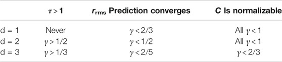
TABLE 1. Behavior with γ in various dimensions d as predicted by Eq. 2.

Interestingly, there exists an alternative route to the solution given in Eq. 5; 11: Working in $d=1$ Plastino and Plastino [41] showed that by adding a drift term to Eq. 1 that corresponds to the force from a harmonic potential, a stationary solution could be found. Using the anzats that the full time-dependent solution has that same structure as the stationary one, only with time-dependent coefficients, the structure of Eq. 5; 11 is established. Later, Tsallis and Bukman [42] established the full analytic solution to this problem, which structurally reduces to Eq. 5; 11 as the strength of the potential is taken to zero.

III Particle Model that Realizes the Non-Linear Diffusion Equation

We will employ two simulation models, both in $d=3$ with $N_p$ random walkers, labeled i, that have positions ${\mathbf{r}}_i\to {\mathbf{r}}_i+\delta {\mathbf{r}}_i$. The particles interact only via the value of C, which is the local population density. The steps are chosen isotropically at each time step; to find their length we need to derive the appropriate Fokker-Planck equation and match it to Eq. 3. For every time step $\text{Δ}t$ the walkers move

$\delta r_{i\alpha }=\eta g\left(C\left({\mathbf{r}}_i\right)\right)\sqrt{\text{Δ}t}(14)$

where α is a Cartesian index and the function $g\left(C\right)$ is to be determined. This defines a Wiener process with η as a random variable with $\langle \eta \rangle =0$ and $\langle {\eta }^2\rangle =1$. Now, following the same steps as in [40, 43] we use the standard Chapman-Kolmogorov, or master equation, to derive the following Fokker-Planck equation for the particle concentration $C\left(\mathbf{r},t\right)$

$\frac{\partial C\left(\mathbf{r},t\right)}{\partial t}=\frac{1}{2}{\nabla }^2\left(a_2\left(\mathbf{r}\right)C\left(\mathbf{r},t\right)\right).(15)$

Here $a_2\left(\mathbf{r}\right)$ is the mean squared jump length per time,

$a_2\left(\mathbf{r}\right)={{\displaystyle \int }}^{\text{}}{d}^{3}x\frac{{\mathbf{x}}^2}{3}W\left(\mathbf{r},\mathbf{x}\right)=\frac{1}{3}\frac{\langle \delta {\mathbf{r}}^2\rangle }{\text{Δ}t}=g{\left(C\right)}^2,(16)$

where $W\left(\mathbf{r},\mathbf{x}\right)$ is the probability per unit time that a walker jumps a distance $\mathbf{x}$ from $\mathbf{r}$. Setting $g\left(C\right)=b{C}^{-\gamma /2}$ gives

$\frac{\partial C}{\partial t}=\frac{b^2}{2}{\nabla }^2{C}^{1-\gamma },(17)$

and requiring equivalence with Eq. 3 thus implies that $b^2=2D_0/\left(C_0^{-\gamma }\left(1-\gamma \right)\right)$. This leads to the step

$\delta r_{\alpha }=\eta \sqrt{\frac{2D_0\text{Δ}t}{\left(1-\gamma \right)}}{\left(\frac{C\left(\mathbf{r},t\right)}{C_0}\right)}^{-\gamma /2}(18)$

where the random variable η is given above.This defines the particle model that is described by Eq. 3.

In the finite interaction range model C is calculated by assuming a maximum interaction range $\text{Δ}x$ between particles. This is done by calculating C onto a lattice with lattice constant $\text{Δ}x$: The local value $C\left({\mathbf{r}}_n,t\right)$ at the discrete site ${\mathbf{r}}_n$ is simply $1/\text{Δ}{x}^d$ times the number of particles at positions ${\mathbf{x}}_i$ that satisfy $|x_{i\alpha }-x_{n\alpha }|<\text{Δ}x/2$. The step length for a particle that is located at $\mathbf{x}$ depends on the C-value at the nearest lattice site. The finite interaction range of this model has a discretization effect: Once C is so small that there is only one- or zero particles in each $\text{Δ}x$ cell, the step length will always be the same, and as a result, there will be a cross-over to normal $r_{rms}\sim t^{1/2}$ diffusion, an effect that is observed in the $\gamma =0.35$ curve of Figure 1A.

FIGURE 1

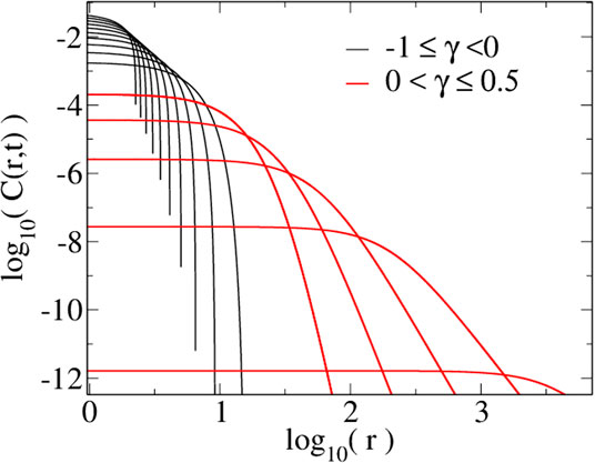
FIGURE 1. (A) Simulations of $r_{rms}$ compared to the theoretical values of Eq. 13 for the finite-interaction range model using $N_p={10}^6$ particles and $D_0=1$. (B)$r_{rms}$ resulting from the infinite-interaction range model using $N_p=1500$ particles. The solid lines show the predicted slope of Eq. 2.

The other, infinite interaction range model employs no lattice at all, but evaluates C at any particle position $\mathbf{x}$ as $C\left(\mathbf{x},t\right)=N_r/V_r\left(\mathbf{x}\right)$ where $N_r\sim 10$ is a fixed particle number and $V_r\left(\mathbf{x}\right)$ is the volume of the sphere that contains $N_r$ nearest neighbors, as illustrated by Figure 2 in the $d=2$ case with $N_r=10$.

FIGURE 2

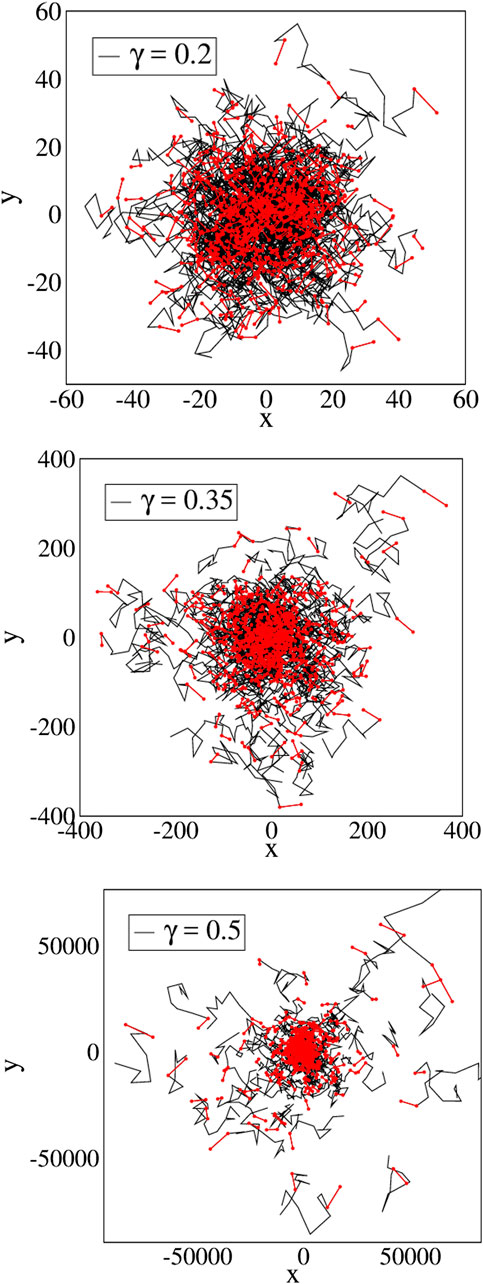
FIGURE 2. The sphere of volume $V_r$ containing the $N_r=10$ particles that defines the local concentration for the central particle.

There is no upper limit to the size of $V_r\left(\mathbf{x}\right)$, and it is in this sense that the model has a potentially infinite interaction range. When $\gamma \ne 0$ this model will never cross over to normal diffusive behavior. A somewhat similar particle, but one-dimensional, particle model was introduced by Borland [44], who in stead of calculating the local C-value from the neighboring particles, employed the analytical solution for C.

In Figure 3 the analytic solution of Eq. 11 is plotted for different γ-values. The term “explosive” seems an appropriate label for the behavior of the concentration for two reasons: First, as $\gamma \to 1/2$ close to the critical value of 2/3, the initial concentration $C\left(\mathrm{0,0}\right)$ drops by more than 10 orders of magnitude in the same time that the negative γ solutions (taken from Pattle [39]), drop by less than two orders. Second, the divergence of the integral in Eq. 8 defining $r_{rms}\left(t\right)$ signals a cross-over to a regime where the break-away particles dominate the $r_{rms}\left(t\right)$ behavior at ever increasing step lengths.

FIGURE 3

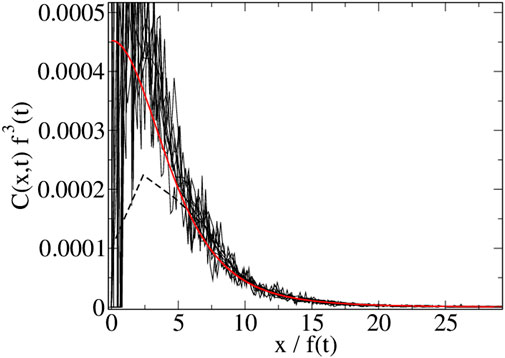
FIGURE 3. The predicted/theoretical concentration field at different γ-values when $D_0=1$ and $t=10$. The black curves show Pattles [39] solution for $\gamma =-0.1,-0.2,-0.4,-0.5$.

Figure 4 show simulations using dimensionless spatial and time coordinates. If units were assigned to them the background diffusivity $D_0$ would have dimension length²/time as usual. The time step $dt=1/N_p^{\gamma }$ is chosen in order to avoid significant changes in the local concentration from time-step to time-step. Note the increasing presence of particles that separate from the main crowd as γ is increased.

FIGURE 4

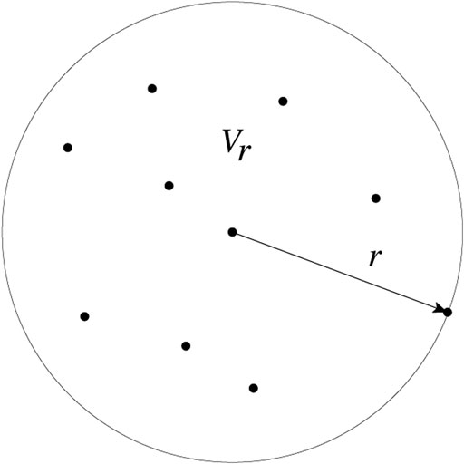
FIGURE 4. Projections into the xy-plane of particle trajectories for different values of γ, using the infinite-interaction-range model. The last 10 time steps are shown in black the last step in red. All simulations are run for a time $t=10$ with $N_p=500$ particles, $dt=1/N_P^{\gamma }$, and $D_0=1$.

In Figure 5 the data collapse anticipated in Eq. 5 is seen to be satisfied. Figures 1A,B demonstrate that the particle displacement is in fact characterized by Eq. 13, the difference between Figures 1A,B, being that the first figure compares simulations and the full analytic prediction of Eq. 13, while the hyperballistic transport shown in Figures 1B, only confirms the prediction of the τ exponent, Eq. 2. Note that in Figures 1A the convergence to the prediction of Eq. 13, happens over a time that increases with γ, signaling the end of the regime where $r_{rms}\left(t\right)$ has an exact analytical expression.

FIGURE 5

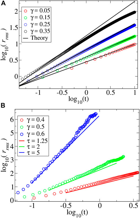
FIGURE 5. Simulations, sampled at equispaced time intervals (the stapled curve shows the first time) using $\gamma =0.4$ and the finite-interaction range model. The curves show $p\left(y\right)=C\left(r,t\right)f^3\left(t\right)$ as a function of $y=r/f\left(t\right)$ compared to theory (red curve) of Eq. 11 and Eq. 12.

Figure 6 summarizes this comparison for the full range of relevant γ-values, using the finite-range model for the smaller- and the infinite range model for the larger γ-values.

FIGURE 6

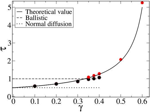
FIGURE 6. Simulation results for τ using the finite range $\left(\text{Δ}x=1\right)$ model for $\gamma \le 0.6$ (black symbols), and the infinite-range model for $\gamma =0.35-0.6$ (red symbols). The full line is the theoretical values.

FIGURE 7

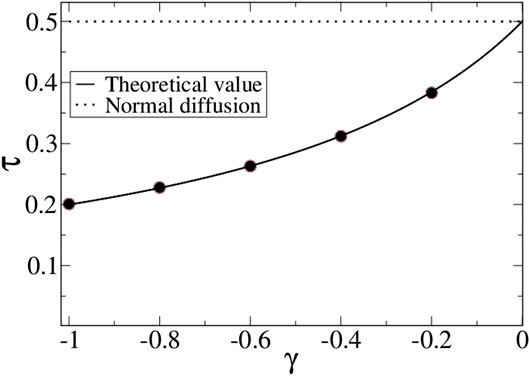
FIGURE 7. Simulation results for τ using the finite range $\left(\text{Δ}x=1\right)$ model for $\gamma \le 0$ values (black symbols). The full line is the theoretical values.

IV Conclusion

In conclusion, we have shown that particle interactions described entirely in terms of their local concentration may yield superdiffusion, and even hyperballistic diffusion. This was done by solving the diffusion equation with the diffusivity $D\sim C^{-\gamma }$ exactly. The particle interactions were described in terms of this concentration dependence alone. Unlike earlier solutions [42, 44] in $d=1$ the present solutions yield hyper-ballistic diffusion. In $d=3$ ($d=2$) this happens when $\gamma >1/3\left(1/2\right)$. The 3-dimensional particle model that was introduced as a realization of this diffusion equation was found to reproduce the exact solution for a range of γ-values, and also the predicted root-mean-square displacement in the range of γ values where this prediction is finite. Notably, also outside this range ($\gamma >0.4$) did the particle simulation confirm the predicted diffusion exponent.

Data Availability Statement

The raw data supporting the conclusions of this article will be made available by the authors, without undue reservation.

Author Contributions

All authors contributed to the analytic work and discussions. EGF did the simulations and the writing of the paper.

Funding

This work was partly supported by the Research Council of Norway through its Centers of Excellence funding scheme, project number 262644.

Conflict of Interest

The authors declare that the research was conducted in the absence of any commercial or financial relationships that could be construed as a potential conflict of interest.

Appendix

In Pattles classical 1959 paper [39] the $\gamma <0$ solution of Eq. 1 is not actually derived, but only written down. So, for completeness we derive it here along the same lines as those leading up to Eq. 11. In the solutions thus derived $C\left(r,t\right)$ has a final support outside which it is strictly zero. For any γ the normalization

$C_d{{{\displaystyle \int }}^{\text{}}}_0^{\infty }dr{r}^{d-1}C\left(r,t\right)=C_d{{{\displaystyle \int }}^{\text{}}}_0^{\infty }dy{y}^{d-1}p\left(y\right)=N_p,(19)$

where we have used the isotropic nature of the problem to perform the angular integration and thus introduced the geometric factor $C_d=\mathrm{1,2}\pi ,4\pi$ when $d=\mathrm{1,2,3}$.

We see from Eq. 11 that, for $\gamma <0$, the domain of the probability density, $p\left(y\right)$, is limited to $y<y_c=\sqrt{2k\left(\gamma -1\right)/\gamma }$, so that the normalization condition is

${{{\displaystyle \int }}^{\text{}}}_0^{y_c}dy{y}^{d-1}p\left(y\right)=\frac{N_p}{C_d}.(20)$

yielding the normalization constant

$k={\left[N_p{\left(\frac{\gamma }{2\pi \left(\gamma -1\right)}\right)}^{\frac{d}{2}}\frac{\text{Γ}\left(\frac{d}{2}+1-\frac{1}{\gamma }\right)}{\text{Γ}\left(1-\frac{1}{\gamma }\right)}\right]}^{\frac{2\gamma }{d\gamma -2}},(21)$

for $\gamma <0$.

We now combine results, using Eqs. 5, 7; 11. to find the concentration field, $C\left(r,t\right)$

$C\left(r,t\right)=\text{Θ}\left(r_c-r\right){\left(\frac{2-d\gamma }{1-\gamma }{D}_0{C}_0^{\gamma }t\right)}^{-\frac{d}{2-d\gamma }}{\left[k-\frac{\gamma }{2\left(\gamma -1\right)}{\left(\frac{2-d\gamma }{1-\gamma }{D}_0{C}_0^{\gamma }t\right)}^{-\frac{2}{2-d\gamma }}{r}^2\right]}^{-\frac{1}{\gamma }},(22)$

where

$r_c={\left(\frac{2k\left(\gamma -1\right)}{\gamma }\right)}^{\frac{1}{2}}{\left(\frac{2-d\gamma }{1-\gamma }{D}_0{C}_0^{\gamma }t\right)}^{\frac{1}{2-d\gamma }},(23)$

By comparison, for $\gamma >0$ we have

$C\left(r,t\right)={\left(\frac{2-d\gamma }{1-\gamma }{D}_0{C}_0^{\gamma }t\right)}^{-\frac{d}{2-\gamma }}{\left[\frac{\gamma }{2\left(1-\gamma \right)}{\left(\frac{2-d\gamma }{1-\gamma }{D}_0{C}_0^{\gamma }t\right)}^{-\frac{2}{2-d\gamma }}{r}^2+k\right]}^{-\frac{1}{\gamma }},(24)$

with k given by Eq. 12 now. Finally we find that for $\gamma <0$, $r_{rms}^2=A{t}^{2\tau }$ with

$A=\frac{{\pi }^{\frac{d}{2}}}{N_p}{k}^{\frac{d}{2}+1-\frac{1}{\gamma }}\frac{d}{2}\frac{\text{Γ}\left(1-\frac{1}{\gamma }\right)}{\text{Γ}\left(\frac{d}{2}+2-\frac{1}{\gamma }\right)}{\left(\frac{2\left(\gamma -1\right)}{\gamma }\right)}^{\frac{d}{2}+1}{\left(\frac{2-d\gamma }{1-\gamma }{D}_0{C}_0^{\gamma }\right)}^{\frac{2}{2-d\gamma }}.(25)$

In Figure 7 this behavior is confirmed by simulations using the finite-range model.

References

1. Bouchaud J, Georges A. Anomalous diffusion in disordered media: statisticalmechanisms, models, and physical applications. Phys Rep (1990) 195:125. doi:10.1016/0370-1573(90)90099-n

CrossRef Full Text | Google Scholar

2. Gosh SK, Cherstvy AG, Grebenkov D, Metzler R. Anomalous non-gaussiantracer diffusion in crowded two-dimensional environments. New J Phys (2016) 18:013027. 10.1088/1367-2630/18/1/013027

Google Scholar

3. Richardson L. Atmospheric diffusion shown on a distance-neighbour graph. Proc Roy Soc London A (1926) 100:709. 10.1098/rspa.1926.0043

Google Scholar

4. Schlesinger M, West B, Klafter J. Levy dynamics of enhanced diffusion: application to turbulence. Rev Geophys (1987) 58:1101. 10.1103/PhysRevLett.58.1100

Google Scholar

5. Ramos-Fernundez G, Mateos J, Miramontes O, Cocho G, Larralde H, Ayala-Orozco B. Levy walk patterns in the foraging movements of spidermonkeys (Ateles geoffroyi). Behav Ecol Sociobiol (2004) 55:223. 10.1007/s00265-003-0700-6

CrossRef Full Text | Google Scholar

6. Viswanathan GM, Afanasyev V, Buldyrev SV, Murphy EJ, Prince PA, Stanley HE. Lévy flight search patterns of wandering albatrosses. Nature (1996) 381:413. doi:10.1038/381413a0

CrossRef Full Text | Google Scholar

7. Viswanathan GM, Buldyrev SV, Havlin S, da Luz MGE, Raposo EP, Stanley HE. Optimizing the success of random searches. Nature (1999) 401:911914. doi:10.1038/44831

CrossRef Full Text | Google Scholar

8. Jayannavar AM, Kumar N. Nondiffusive quantum transport in a dynamically disordered medium. Phys Rev Lett (1982) 48:553. doi:10.1103/physrevlett.48.553

CrossRef Full Text | Google Scholar

9. Golubovic L, Feng S, Zeng FA. Classical and quantum superdiffusion in a time-dependent random potential. Phys Rev Lett (1991) 67:2115. doi:10.1103/PhysRevLett.67.2115

PubMed Abstract | CrossRef Full Text | Google Scholar

10. Levi L, Krivolapov Y, Fishman S, Segev M. Hyper-transport of light and stochastic acceleration by evolving disorder. Nat Phys (2012) 8:912. doi:10.1038/nphys2463

CrossRef Full Text | Google Scholar

11. Sagi Y, Brook M, Almog I, Davidson N. Observation of anomalous diffusion and fractional self-similarity in one dimension. Phys Rev Lett (2012) 108:093002. doi:10.1103/physrevlett.108.093002

PubMed Abstract | CrossRef Full Text | Google Scholar

12. Anderson PW. Absence of diffusion in certain random lattices. Phys Rev (1958) 109:1492. doi:10.1103/physrev.109.1492

CrossRef Full Text | Google Scholar

13. Muskat M. The flow of fluids through porous media. J Appl Physics (1937) 8:274. doi:10.1063/1.1710292

CrossRef Full Text | Google Scholar

14. Barenblatt GI, Entov VM, Ryzhik VM. Theory of fluid flows through natural rocks, Vol. ber90. Dordrecht, Netherland: Kluwer (1990). 396 p.

15. Hurtado PI, Krapivsky PL. Compact waves in microscopic nonlinear diffusion. Phys Rev E (2012) 85:060103. doi:10.1103/physreve.85.060103

CrossRef Full Text | Google Scholar

16. Kamenomostskaya SK. Similar solutions and the asymptotics of filtration equations. Arch Rational Mech Anal (1976) 60, 171. doi:10.1007/bf00250678

CrossRef Full Text | Google Scholar

17. Zeldovich IB, Kompaneez AS. “On the theory of heat propagation with heatconduction depending on temperature,” in Lectures dedicated on the 70th anniversary of A. F. Joffe. Moscow, Russia: Akad. Nauk SSSR (1950). p. 61–71.

Google Scholar

18. Zeldovich Y, Raizer YP. Physics of shock waves and high-temperature hydrodynamic phenomena, Vol. 2. New York, NY: Academic Press (1968). p. 826–7.

19. Gurtin ME, MacCamy RC. On the diffusion of biological populations. Math Biosci (1977) 33:35. doi:10.1016/0025-5564(77)90062-1

CrossRef Full Text | Google Scholar

20. Newman WI. Some exact solutions to a non-linear diffusion problem in population genetics and combustion. J Theor Biol (1980) 85:325. doi:10.1016/0022-5193(80)90024-7

PubMed Abstract | CrossRef Full Text | Google Scholar

21. Murray JD. Mathematical biology, m89, biomathematics. Berlin, Germany: Springer (1989). 770 p.

22. de Azevedo EN, de Sousa PL, de Souza RE, Engelsberg M, Miranda MDNDN, Silva MA. Concentration-dependent diffusivity and anomalous diffusion: a magnetic resonance imaging study of water ingress in porous zeolite. Phys Rev E (2006a) 73:011204. doi:10.1103/physreve.73.011204

CrossRef Full Text | Google Scholar

23. de Azevedo EN, da Silvaandde Souzaand DV, Engelsberg RE, Engelsberg M. Water ingress in y-type zeolite: anomalous moisture-dependent transport diffusivity. Phys Rev E(2006b) 74:041108. doi:10.1103/physreve.74.041108

CrossRef Full Text | Google Scholar

24. Fischer D, Finger T, Angenstein FRSR. Diffusive and subdiffusive axial transport of granular material in rotating mixers. Phys Rev E (2009) 80:061302. doi:10.1103/physreve.80.061302

CrossRef Full Text | Google Scholar

25. Stannarius IC, Has HA. Resolving a paradox of anomalous scalings in the diffusion of granular materials. Proc Natl Acad Sci (2012) 109:16012. doi:10.1073/pnas.1211110109

PubMed Abstract | CrossRef Full Text | Google Scholar

26. Stone D, Woods AW, Hogg AJ. On the slow draining of a gravity current moving through a layered permeable medium. J Fluid Mech (2001) 444:23. doi:10.1017/s002211200100516x

CrossRef Full Text | Google Scholar

27. Hansen A, Skagerstam B-S, Tørå G. Anomalous scaling and solitary waves in systems with nonlinear diffusion. Phys Rev E (2011) 83:056314. doi:10.1103/physreve.83.056314

CrossRef Full Text | Google Scholar

28. Shlesinger MF. Asymptotic solutions of continuous-time random walks. J Stat Phys (1974) 10:421. doi:10.1007/bf01008803

CrossRef Full Text | Google Scholar

29. Havlin S, Kiefer JE, Weiss GH. Anomalous diffusion on a random comblike structure. Phys Rev A (1987) 36:1403. doi:10.1103/physreva.36.1403

CrossRef Full Text | Google Scholar

30. Havlin S, Djordjevic ZV, Majid I, Stanley HE, Weiss GH. Relation between dynamic transport properties and static topological structure for the lattice-animal model of branched polymers. Phys Rev Lett (1984) 53:178. doi:10.1103/physrevlett.53.178

CrossRef Full Text | Google Scholar

31. de Gennes PG. La percolation un concept unificateur, La Recherche. Singapore: World Scientific Publishing (1976). 919 p.

32. ben-Avraham D, Havlin S. Diffusion and reactions in fractals and disordered systems. London, United Kingdom: Cambridge University Press (2000). 316 p.

33. ben-Avraham D, Leyvraz F, Redner S. Superballistic motion in a “random-walk” shear flow. Phys Rev A (1992) 45:2315. doi:10.1103/physreva.45.2315

PubMed Abstract | CrossRef Full Text | Google Scholar

34. ben-Naim E, Redner S, ben-Avraham D. Bimodal diffusion in power-law shear flows. Phys Rev A (1992) 45:7207. doi:10.1103/physreva.45.7207

PubMed Abstract | CrossRef Full Text | Google Scholar

35. Schütz GM, Trimper S. Elephants can always remember: exact long-range memory effects in a non-markovian random walk. Phys Rev E (2004) 70:045101. doi:10.1103/physreve.70.045101

CrossRef Full Text | Google Scholar

36. Morgado R, Oliveira FA, Batrouni GG, Hansen A. Relation between anomalous and normal diffusion in systems with memory. Phys Rev Lett (2002) 89:100601. doi:10.1103/physrevlett.89.100601

PubMed Abstract | CrossRef Full Text | Google Scholar

37. Wei X, Bauer W. Starvation-induced changes in motility, chemotaxis, and flagellation of rhizobium melilot. Appl Abd Environ Microbiol (1998) 65:1708–14. doi:10.1128/AEM.64.5.1708-1714.1998

CrossRef Full Text | Google Scholar

38. Wu X-L, Libchaber A. Particle diffusion in a quasi-two-dimensional bacterial bath. Phys Rev Lett (2000) 84:3017. doi:10.1103/physrevlett.84.3017

PubMed Abstract | CrossRef Full Text | Google Scholar

39. Pattle RE. Diffusion from an instantaneous point source with a concentration-dependent coefficient. Q J Mech Appl Math (1959) 12:407. doi:10.1093/qjmam/12.4.407

CrossRef Full Text | Google Scholar

40. Hansen A, Flekkøy EG, Baldelli B. Anomalous diffusion in systems with concentration-dependent diffusivity: exact solutions and particle simulations. Front Phys (2020) 8:519624. doi:10.3389/fphy.2020.519624

CrossRef Full Text | Google Scholar

41. Plastino AR, Plastino A. Non-extensive statistical mechanics and generalized Fokker-Planck equation. Physica A (1995) 222:347. doi:10.1016/0378-4371(95)00211-1

CrossRef Full Text | Google Scholar

42. Tsallis C, Bukman DJ. Anomalous diffusion in the presence of external forces: exact time-dependent solutions and their thermostatistical basis. Phys Rev E (1996) 54:R2197. doi:10.1103/physreve.54.r2197

CrossRef Full Text | Google Scholar

43. van Kampen N. Stochastic processes in physics and chemistry. 3rd ed, Vol. k07. Amsterdam: North Holland (2007). 464 p.

44. Borland L. Microscopic dynamics of the nonlinear Fokker-Planck equation: a phenomenological model. Phys Rev E (1998) 57:6634. doi:10.1103/physreve.57.6634

CrossRef Full Text | Google Scholar