Data Mining Reconstruction of Magnetotail Reconnection and Implications for Its First-Principle Modeling

Magnetic reconnection is a fundamental process providing topological changes of the magnetic field, reconfiguration of space plasmas and release of energy in key space weather phenomena, solar flares, coronal mass ejections and magnetospheric substorms. Its multiscale nature is difficult to study in observations because of their sparsity. Here we show how the lazy learning method, known as K nearest neighbors, helps mine data in historical space magnetometer records to provide empirical reconstructions of reconnection in the Earth’s magnetotail where the energy of solar wind-magnetosphere interaction is stored and released during substorms. Data mining reveals two reconnection regions (X-lines) with different properties. In the mid tail ($\sim 30R_E$ from Earth, where $R_E$ is the Earth’s radius) reconnection is steady, whereas closer to Earth ($\sim 20R_E$) it is transient. It is found that a similar combination of the steady and transient reconnection processes can be reproduced in kinetic particle-in-cell simulations of the magnetotail current sheet.

1 Introduction

Charged particles, electrons and ions forming space plasmas usually drift in the ambient magnetic field making plasmas frozen in that field [1]. The frozen-in condition may be broken when oppositely directed field lines approach each other so closely that particles become unmagnetized and their orbits become different from conventional drift motions. As a result, magnetic field lines may change their connectivity near so-called X-lines in the process of magnetic reconnection. This process was introduced to explain major sources of space weather disturbances on the Sun, solar flares [2, 3] and coronal mass ejections (CMEs) [4]. It was also invoked by Dungey [5] to describe the structure of the Earth’s magnetosphere, the plasma bubble surrounding our planet and protecting its life from the hazardous stream of high-energy particles emitted by our star. According to Dungey, reconnection takes place on the day side of the magnetospheric boundary, the magnetopause, to provide the solar wind plasma entry into the magnetosphere through the reconnected magnetic flux tubes. Then the flux tubes reconnect again on the night side, in the region where the Earth’s dipole magnetic field lines are stretched in the antisunward direction forming the magnetotail. Finally, to explain a delayed explosive response of the polar regions of the magnetosphere to solar wind disturbances during substorms [6], Hones [7] proposed that the substorm explosions are powered by the unsteady reconnection in the tail due to the formation of another “near-Earth” X-line.

The magnetotail reconnection is important not only as a key element of the space weather chain. It occurs in space plasma practically in the absence of particle collisions. Similar collisionless reconnection processes are expected to occur in the solar corona during flares and CMEs, where in-situ observations are impossible [1]. They are also expected in sufficiently hot laboratory plasmas that are investigated on the way to controlled nuclear fusion [8]. Thus, the magnetotail represents a natural space laboratory for collisionless reconnection due to many dedicated missions, such as Geotail [9], Cluster [10], THEMIS [11] and MMS [12].

The magnetotail is also very interesting because it reveals different regimes of reconnection. On the one hand, it must experience steady reconnection, which was conjectured by Dungey [5] in his description of the magnetospheric convection cycle and later confirmed in observations of steady magnetospheric convection (SMC) regimes [13]. On the other hand, the magnetotail experiences unsteady reconnection during substorms [7].

Both the first-principle modeling and the empirical reconstruction of magnetotail reconnection are very difficult to perform because of its multiscale nature. It links global reconfigurations of the nightside magnetosphere to kinetic processes on the scales of ion or even electron gyroradii that provide irreversibility for global reconfigurations. As a result, its kinetic particle-in-cell (PIC) simulations describing the full dynamics of electrons and ions (largely protons) and their self-consistent electromagnetic fields [14] are usually limited to the immediate X-line vicinity [15] and the moments after the X-line formation in global magnetohydrodynamic models [16], where the reconnection onset is provided due to numerical or ad hoc plasma resistivity. Moreover, it is very difficult to take into account that the magnetotail itself becomes multiscale prior to the reconnection onset. In-situ observations suggest that it may contain thin (ion-scale) current sheets (TCS) embedded into a thicker current sheet (CS) [17–21]. The latter may also be split in two current layers forming bifurcated TCSs [19, 22–24].

The major problem in the empirical reconstruction of magnetotail reconnection, common to all in-situ space observations, is the extreme sparsity of these observations with fewer than a dozen probes available at any moment. To solve this problem, it has recently been proposed to mine data in the multi-mission database covering many years of historical spaceborne magnetometer observations [25, 26]. It was found that such a data-mining (DM) method resolves the formation of embedded TCSs in the growth phase of substorms and their decay after the substorm onset. It also resolves the formation of the near-Earth X-lines during substorms [27]. Here we show that the DM approach allows one to resolve the formation of two different X-lines in the magnetotail during substorms. Moreover, it becomes possible to quantitatively assess their steadiness. We also show that PIC simulations guided by the DM reconstruction of the magnetotail reproduce the formation of X-lines and reconnection regimes similar to those found in the DM analysis.

2 Data Mining Method

In the DM approach, the geomagnetic field is reconstructed using not only a few points of spaceborne magnetometer measurements available at the moment of interest, but also a much larger number of other measurements made at the $K_{NN}\gg 1$ moments in the past. These moments called “the nearest neighbors” or NNs are similar to the event of interest in terms of similar values of the geomagnetic indices Sym-H and AL, their time derivatives and the solar wind input parameter $v{B}_s^{IMF}$. Here $B_s^{IMF}$ is the southward component of the Inteplanetary Magnetic Field (IMF): $B_s^{IMF}=-B_z^{IMF}$ if $B_z^{IMF}<0$ and $B_s^{IMF}=0$ otherwise (The Geocentric Solar Magnetospheric coordinate system (GSM) coordinate system is used throughout this paper. Its origin is at the center of the Earth; the X-axis is directed toward the Sun; the y-axis is defined as the cross product of the GSM x-axis and the magnetic dipole axis, directed positive toward dusk; the z-axis is defined as the cross product of the x- and y-axes.) The large number of NNs is at the same time much smaller than the size of the database $K_{DB}\gg K_{NN}$. This allows one to fit with the NN subset a complex empirical magnetic field model [26], and at the same time, to make the model reconstructions sufficiently flexible to reflect the characteristic variations of the magnetosphere during storms and substorms.

This approach resembles very much the “lazy-learning” pattern recognition technique known as the K-nearest neighbor (KNN) learning [28, 29]. At the same time, our DM approach differs from conventional KNN regression methods, where both finding the NNs (“mining”) and regressions (model fitting) are made in the same space. Here, as is illustrated in Figure 1, we first detect NNs as a (sub)set of $K_{NN}$ present and historical moments in similar phases of similar substorms. Their similarity (“neighborhood”) is quantified by the closeness of the corresponding global magnetospheric activity parameters and their time derivatives to their values at the moment of interest (Figure 1A). Then we use these $K_{NN}$ moments to form an event-oriented subset of the original database of magnetic field observations (Figure 1B) and to fit our magnetic field model with this subset (Figure 1C).

FIGURE 1

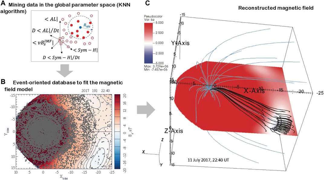
FIGURE 1. DM algorithm of the magnetic field reconstruction used in this study: (A) Nearest neighbor selection using KNN method. (B) The event-oriented subset of the database formed using the selected set of $K_{NN}$ nearest neighbors. It is used to fit the magnetic field model. Gray dots show the projections of the spacecraft coordinates on the equatorial plane, where the normal magnetic field component $B_z$ is color coded. (C) The resulting magnetic field lines (black) and the equatorial field $B_z$ (color-coded) assuming zero tilt angle (adapted from [27]).

The NN subset is formed by points $G^{\left(i\right)}=\left[G_1\left(t_i\right),\dots ,G_5\left(t_i\right)\right]$, $i=1,\dots K_{NN}$, in the 5-D space that are closest to the query point (moment of interest $t_q$) $G^{\left(q\right)}=\left[G_1\left(t_q\right),\dots ,G_5\left(t_q\right)\right]$ by the Euclidean metric

$R_q^{\left(i\right)}=\sqrt{{\displaystyle \sum _{k=1}^5{\left(G_k^{\left(i\right)}-G_k^{\left(q\right)}\right)}^2/{\sigma }_{G_k}^2}}.(1)$

where ${\sigma }_{G_k}$ is the standard deviation of the component $G_k$ and the coordinates $G_1$-$G_5$ are defined by the formulae:

$G_1\left(t\right)=\langle Sym-H^{\text{*}}|\propto {\displaystyle {\int }_{-{\text{Π}}_{st}/2}^{0}Sym-H^{\text{*}}\left(t+\tau \right)\text{cos}\left(\pi \tau /{\text{Π}}_{st}\right)d\tau }(2)$

$G_2\left(t\right)=D\langle Sym-H^{\text{*}}|/Dt\propto {\displaystyle {\int }_{-{\text{Π}}_{st}/2}^{0}Sym-H^{\text{*}}\left(t+\tau \right)\text{sin}\left(2\pi \tau /{\text{Π}}_{st}\right)d\tau }(3)$

$G_3\left(t\right)=\langle AL|\propto {\displaystyle {\int }_{-{\text{Π}}_{sst}/2}^{0}AL\left(t+\tau \right)\text{cos}\left(\pi \tau /{\text{Π}}_{sst}\right)d\tau }(4)$

$G_4\left(t\right)=D\langle AL|/Dt\propto {\displaystyle {\int }_{-{\text{Π}}_{sst}/2}^{0}AL\left(t+\tau \right)\text{sin}\left(2\pi \tau /{\text{Π}}_{sst}\right)d\tau }(5)$

$G_5\left(t\right)=\langle v{B}_s^{IMF}|\propto {\displaystyle {\int }_0^{{\tau }_{\infty }}v{B}_s^{IMF}\left(t-{\tau }_{\infty }+\tau \right)\text{exp}\left[\left(\tau -{\tau }_{\infty }\right)/{\tau }_0\right]d\tau }(6)$

Here $Sym-H^{\text{*}}=A\cdot Sym-H-B\cdot \sqrt{P_{dyn}}$ is the pressure-corrected Sym-H index [30], $P_{dyn}$ is the solar wind dynamic pressure (in nPa) and the values of A and B are taken to be 0.8 and 13.0, respectively. The functions $G_1$ and $G_3$ in Eqs. 2, 4 describe weighted moving averages of the indices Sym-H and $AL$ limited to their past values (see [25] for further details), while $G_2$ and $G_4$, defined by Eqs. 3, 5, describe the corresponding smoothed time derivatives. Weighting in moving averages (2–5) is provided by the sine and cosine kernel functions and by the exponential function in Eq. 6. The averaging scaling parameters ${\text{Π}}_{st}=12\mathrm{hr}$ and ${\text{Π}}_{sst}=2\mathrm{hr}$ reflect the characteristic storm and substorm scales. The parameter $G_5$ defined by Eq. 6 describes the integral effect of the magnetic flux accumulation in the tail during the growth phase due to the dayside reconnection. Its scale ${\tau }_0=0.5\mathrm{hr}$ is selected based on observed values of a typical growth phase duration [31]. The selected upper integration limit in Eq. 6${\tau }_{\infty }=6{\tau }_0$ corresponds to six e-folding times.

In the 5-D space of the binning parameters (2)–(6), the $AL$ index and its time derivative $\left(G_3,G_4\right)$ determine the strength and phase of the substorm activity, because the $AL$ index reflects the strength of the substorm electrojet [32]. These parameters may still be insufficient to capture the substorm growth phase, which is characterized by the accumulation of the magnetic flux in the tail lobes without any significant electrojet enhancement. To take this effect into account, we involve in the analysis the solar wind electric field parameter through the binning variable $G_5$. Furthermore, many substorms occur at the moments of the storm activity, which may substantially modify the substorm evolution of the magnetosphere [33]. To take these effects into account, we further extend the binning space at the expense of the parameters $G_1$ and $G_2$ reflecting the storm-time index Sym-H and its time derivative (to distinguish between main and recovery storm phases).

The conjecture that the substorm dynamics of the magnetosphere is coherent and hence the distribution of its magnetic field can be determined by a few control parameters had been formulated many years ago (e.g., [34], and refs. therein). Later, the singular spectrum analysis of substorms [35] revealed that the mean-field dynamics of the magnetosphere can be described as a motion on a folded 2-D surface in a 3-D state space formed by the average $AL$ index, average $v{B}_s^{IMF}$ parameter and its average time derivative. An increase of the dimensionality through the Sym-H index and its time derivative, to take magnetic storms into account and to distinguish between their main and recovery phases, is consistent with the original DM-based storm-time model, TS07D [36]. The latter was also justified by the empirical relationship between the $v{B}_s^{IMF}$ parameter and the $Dst$ index, a 1-h time resolution analog of Sym-H [37]. Independent description of storms and substorms assuming their common solar wind driver is consistent with recent analysis of the storm-substorm relationship using a multivariate information-theoretic approach [38]. The further increase of state space dimensionality (e.g., using higher time derivatives of storm and substorm indices as well as the solar wind input parameter) is also possible (e.g., [25]). However, it was found [39] that the effect of higher dimensions often resembles the second-order phase transition fluctuations that require a probabilistic description of the magnetospheric states [40].

The database consists of $K_{DB}=\mathrm{3,668,101}$ records of the magnetic field vector with 5 and 15-min cadence inside and outside $5R_E$, respectively, in archived data from IMP-8, Geotail, Polar, GOES-08, GOES-09, GOES-10, GOES-12, Cluster, THEMIS, Van Allen Probes and MMS missions covering more than two decades (1995–2017) of observations. The KNN subsets are selected using $AL$, Sym-H and $v{B}_s^{IMF}$ time series with 5-min cadence. At every moment $t_q$, the subset is found as $K_{NN}$ points $i=1,\dots ,K_{NN}$ satisfying the condition $R_q^{\left(i\right)}<R_{NN}\left(K_{NN}\right)$, where $R_q^{\left(i\right)}$ is defined by Eq. 1, as is illustrated in Figure 1A. Since the resulting magnetic field geometry is determined by the instantaneous KNN swarm of virtual probes, its time resolution is largely determined by the global parameter cadence. This is seen, for instance, from rapid substorm dipolarizations reproduced by the KNN method in [27] (Fig. 8i), when the $B_z$ field increases from 3 to 10 nT in 5 min over a significant part of the magnetotail. It was found [26, 27] that the use of NN subsets with $K_{NN}\sim \mathrm{32,000}$ and the magnetic field model parameters specified below provides both sufficient selectivity of the model, which allows one to distinguish different substorm phases, and the high spatial resolution to resolve the distinctive features of the magnetospheric morphology in these phases, such as TCSs (and their buildup and decay), flux accumulation regions and X-lines. Smaller $K_{NN}$ values were found to cause overfitting.

At every moment of interest $t_q$, the $K_{NN}$ subset of the database, whose elements neighbor $t_q$ in the state and input space of the magnetosphere by the metric (1), is used to fit the geomagnetic field model SST19 [26]. Since $K_{NN}\gg 1$, its architecture can be made quite complex and flexible (compared, for instance, with the event-oriented models using only a few points of data available at the moment of interest [41, 42]) to capture key features of the substorm current system. In fact, we only assume that the magnetic field is formed by two major current systems inside the magnetosphere, equatorial and field-aligned currents, whose contributions are presented as sums of basis functions with the corresponding amplitude coefficients (more general 3-D expansions of the magnetic field using radial basis functions were considered in [43]). Moreover, to describe the multi-scale structure of the equatorial currents, including the formation of embedded and bifurcated TCSs, these currents are described by two independent expansions:

$B^{\left(eq\right)}\left(\rho ,\varphi ,z\right)=B^{\left(eq\right)}\left(\rho ,\varphi ,z;D\right)+B^{\left(eq\right)}\left(\rho ,\varphi ,z;D_{TCS}\right)(7)$

where $\left(\rho ,\varphi ,z\right)$ are cylindrical coordinates in a system with the origin at the center of the Earth and the z axis normal to the equatorial plane. They represent the magnetic field of thick and thin current sheets with the same structure determined by the approximate solution for the magnetic field of an arbitrary distribution of equatorial currents [44] with different thickness parameters D and $D_{TCS}$ to be derived from the fitting with the NN subset. Each expansion is a finite-sum approximation of an integral solution of the Ampère’s equation for the magnetic field of an infinitely thin CS ($D=0$) above and below the equatorial plane $z=0$ by separation of variables. Tsyganenko and Sitnov [44] showed that the sum consists of N azimuthally symmetric radial expansions and $2M$ angular Fourier harmonics (even and odd parity in ϕ) with the total number of $N+2M\cdot N$ elements. The basis functions of the solution for the vector potential with an infinitely thin CS contain factors like $\text{exp}\left(-k\left|z\right|\right)$. Their regularization comes from assuming the finite CS half-thickness D and it can be provided by replacing the function $\left|z\right|$ by the smooth function $\zeta =\sqrt{z^2+D^2}$. The radial expansions include Bessel functions and they can be exemplified by the azimuthal component $A_{\varphi }$ of the vector potential corresponding to the azimuthally symmetric group of basis functions $B_{0n}^{\left(s\right)}$: ${\left(A_{\varphi }\right)}_{0n}^{\left(s\right)}=J_1\left(k_n\rho \right)\text{exp}\left(-k_n\sqrt{z^2+D^2}\right)$, where $J_1$ is the Bessel function of the first order, $k_n=n/{\rho }_0$, and ${\rho }_0$ is the radial scale, corresponding to the largest mode in the radial expansion.

The parameters ${\rho }_0$, N and M are fixed because they determine the adopted resolution of the expansions in Eq. 7. Other parameters, such as the weights of individual radial and azimutal harmonics, as well as the CS thickness parameters D and $D_{TCS}$, are determined from fitting the model to data. In particular, to distinguish between thick current sheets and TCS, we impose the condition $D_{TCS}<D_{TCS}^{\left(\text{max}\right)}=1R_E$. The latter value is intermediate between the observed thick and thin current sheet values [19] and it does not significantly constrain the specific values of D and $D_{TCS}$ inferred from data. Thus, the spatial resolution of such an expansion is determined by the number of terms in expansions (7) and can be increased to any desired level, commensurate with the data density. To take the global scaling of currents due to variations of the solar wind dynamic pressure $P_{dyn}$ into account, each amplitude coefficient in expansions (7) is further expanded in two parts, one of which is constant and another is a linear function of $\sqrt{P_{dyn}}$. The equatorial expansion has several other nonlinear parameters to take into account global deformations of the tail CS along the dawn-dusk direction and arising from the finite dipole tilt angle, which are described in [44].

Another major group of currents are the field-aligned currents (FACs), connecting the ionosphere with the magnetopause and the tail CS. It is described in SST19 using a similar system of finite current elements [45], sufficiently flexible to reproduce the spiral FAC structure at low latitudes [46] whose night-side part is likely associated with the Harang discontinuity [47]. Each element of the FAC system is described as the magnetic field of two deformed conical surfaces corresponding to Region 1 (R1) and Region 2 (R2) FACs [48]. The size of each system is an adjustable parameter, while their azimuthal distribution is controlled by the relative contributions of two groups of basis functions with odd and even symmetry due to factors $\text{sin}\left(l\varphi \right)$ and $\text{cos}\left(l\varphi \right)$, ($l=\mathrm{1,2},\dots$). The first group represents the main part of the FAC system, in which the dusk-side currents have the same magnitude but opposite direction to those at dawn, while the second group has an even distribution of currents with respect to the noon-midnight meridian plane, which allows one to model the azimuthal rotation of the FACs.

Originally two groups of such FAC elements were proposed in [44] to describe R1 and R2 systems in their DM-based storm-time model, TS07D [36]. Later, it was proposed [45] to use more elements similar to the original TS07D FAC basis functions, shifted in latitude to describe more complex FAC distributions. Eventually, Stephens and coauthors [26] showed that the FAC system can be described with many details important for substorm reconstructions, including the Harang discontinuity and the substorm current wedge [49], with the following set of elements. It consists of $N_{FAC}=16$ basis functions with the first two Fourier harmonics ($l=\mathrm{1,2}$) for R1 and R2, as well as their latitude-shifted clones. Each element in equatorial and FAC expansions is independently shielded (has its own subsystem of Chapman-Ferraro-type currents at the magnetopause).

Thus, the resulting DM algorithm, which links the SST19 model with KNN binning, represents a typical “gray box” model combining empirical algorithms with physics-based constraints [50]. As is shown in [26, 27], it reproduces the multiscale CS thinning process with the formation of an ion-scale TCS ($D_{TCS}\ll 1R_E$) inside a much thicker CS ($D>2R_E$), which takes place in the substorm growth phase and causes stretching of the tail magnetic field lines in the antisunward direction. In particular, Figs. 11a–11c in [27] show the current distribution in the equatorial plane during the growth phase of the 13 February 2008 substorm discussed below. The corresponding current distributions in the meridional plane presented in their Figs. 12a–12c reveal the multiscale CS structure with an ion-scale TCS embedded into a thick CS halo. The peak TCS current density ∼8 nA/m² is consistent with in-situ Cluster observations (see, for example, Figs. 2–4 and 9 in [19]). Further quantitative analysis made in [27] showed that while the TCS thickness in DM reconstructions remains approximately constant $D_{TCS}\approx 0.2R_E$ (Fig. 8e), consistent with Cluster and THEMIS observations [19, 20, 51], their strength (measured as the TCS contribution to the total tail current) changes drastically with the substorm phase (Fig. 12d). At the same time, the contribution of the TCS to the total tail current is relatively small (≈ 1/6). It is worth noting that, as is seen from the comparison of Figs. 10a and 11a in [27], the extended TCS forms earthward of the flux accumulation region ($B_z$ hump).

The DM SST19 algorithm also describes the magnetic field dipolarization in the expansion phase (see, for example, Fig. 4 in [26]) with the formation of a substorm current wedge seen as a curl of the difference between the expansion and growth phase magnetic field distributions ([26], Fig. 10). The disappearance of TCS after the dipolarization can be seen, for instance, from the comparison of Fig. 12d in [27] with other panels in Fig. 12. It can also been seen from their Fig. 8f, where the relative strengths of thin and thick CSs are quantified by integrating the current density over the regions $\left|z\right|<1R_E$ and $\left|z\right|<5R_E$.

The new DM reconstruction has a characteristic property of machine learning algorithms [29, 52]: given more data in the database it may provide more details about the magnetospheric structure and evolution. In particular, as is shown in [27], with adding to the database first two years of the MMS mission data (2016–2017), it becomes possible for the same SST19 model with the parameters $\left(M,N\right)=\left(\mathrm{6,8}\right)$ and $K_{NN}=\mathrm{32,000}$ to resolve more details of the magnetotail structure and evolution. In particular, the 2017 MMS data help resolve the X-lines forming largely beyond $20R_E$, where the pre-MMS database had a substantial drop in the occurrence rate distribution ([27], Fig. 1). This is seen in particular, from the comparison of the SST19 validation using THEMIS data beyond $20R_E$ in Fig, 2e of [26] with THEMIS validation in a similar region in Fig. S6 of [27]. The former reveals clear signatures of overfitting while the latter does not. In spite of a relatively small total number of the new MMS data, they fill the main gap in the existing database distribution ([27], Fig. 1) and thus become particularly important in solving the overfitting problem.

3 13 February 2008 Substorm: Steady and Unsteady X-Lines

In this section we describe the global structure and dynamics of reconnection on the example of a relatively small and short substorm (13 February 2008 02:05–02:55 UT) considered earlier in [27] with the reconstruction parameters $\left(M,N\right)=\left(\mathrm{6,8}\right)$, $K_{NN}=\mathrm{32,000}$ and $N_{FAC}=16$. The latter analysis is extended here by increasing the maximum radial distance of the spacecraft data used in the reconstruction from $31R_E$ to $35R_E$ (largely, due to IMP8 data). Figure 2 shows the equatorial magnetic field distribution at the moment 02:40 UT in the expansion phase of this substorm. It reveals the formation of two X-lines $X_n$ and $X_m$ in the near-Earth ($x\approx -20R_E$) and midtail ($x<-27R_E$) regions, respectively. They are seen as earthward parts of the $B_z=0$ contours in the distribution of the equatorial north magnetic field component $B_z$ in Figure 2 and they are additionally marked by blue arrows. The tailward parts of the $B_z=0$ contours represent O-lines.

FIGURE 2

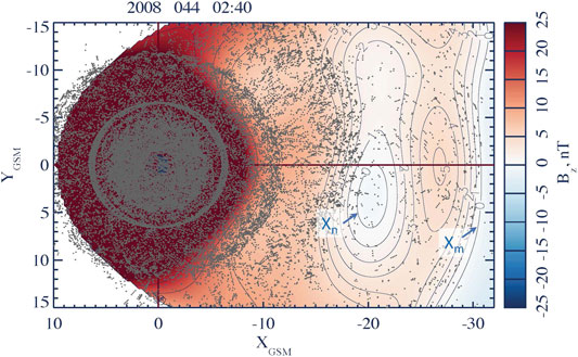
FIGURE 2. Two X-lines, $X_n$ and $X_m$ resolved in the equatorial distribution of the magnetic field $B_z$ (using 0-degree tilt angle for the sake of visualization simplicity) as earthward parts of the contours $B_z$ in case of the 13 February 2008 substorm. The format of this figure is similar to that of Figure 1B. The projections of the spacecraft coordinates on the equatorial plane (gray dots) show that the NN subset of data for the moment considered is sufficient to resolve both X-lines.

This global X-line reconstruction is quite unique. In fact, because of the extreme sparsity of in-situ space observations, such reconstructions were not available before the machine learning era. Earlier, Nagai et al. [53, 54] described the location and the dawn-dusk extension of X-lines using single-point observations. More recently, the reconstructions of the X-line vicinity were made by processing multi-probe MMS data with Grad-Shafranov [55] and polynomial [56] techniques. However, these were still very local reconstruction, largely limited to the size of the MMS tetrahedron (<30 km). Here we demonstrate for the first time how the DM approach based on the KNN algorithm resolves simultaneously two X-lines in the near-Earth and midtail regions.

The formation of transient near-Earth X-lines, which was proposed by Hones [7] as a mechanism of substorms, has been discussed since that time in many studies, including correlated multi-probe and remote sensing analyses (see, for instance [57, 58], and references therein). At the same time, persistent reconnection in the midtail around $30R_E$ follows from THEMIS and ARTEMIS statistics of traveling compression regions [59, 60]. However, neither the co-existence of the second, midtail X-line $X_m$ with $X_n$ nor its relatively steady reconnection, as suggested by Dungey’s convection cycle [5], have ever been demonstrated. Here we not only resolve two X-lines in the tail but also propose a method to quantify their steadiness.

This can be done using the Faraday’s law, which in the 2-D picture of reconnection takes the form

$\partial E_y/\partial x=-\partial B_z/\partial t,\partial E_y/\partial z=\partial B_x/\partial t,(8)$

It suggests that the temporal variations of $B_x$ and $B_z$ magnetic field components determine the spatial gradients of the dawn-dusk (reconnection) electric field. If the magnetic field varies slowly, the corresponding reconnection electric field is broadly distributed over the whole reconnection region. This justifies the concept of the reconnection rate, one of the key global parameters characterizing steady reconnection regimes [61–63]. Reconnection can also be unsteady with the electric field being localized in space and the magnetic field changing in time consistent with (8). For example, Sitnov and Swisdak [64] showed reconnection regimes with the electric field localized near dipolarization fronts (DFs) [65–67] with their values strongly exceeding the steady reconnection values. Localization of the dawn-dusk component of the electric field near DFs was later confirmed by Cluster [68] and THEMIS [69] observations.

The noon-midnight meridional maps of magnetic field lines presented in Figures 3, 4 reveal interesting distinctions of magnetic reconnection in the mid tail region and closer to Earth ($X_m$ and $X_n$ vicinities) in this substorm. As is seen from the comparison of solid and dashed field lines in these figures, reconnection near $X_n$ is accompanied by strong changes of the magnetic field geometry, especially, earthward of that X-line, while near $X_m$ the geometry barely changes, which is seen particularly well in the lobe region. The color-coded variations of the z- and x-components of the magnetic field between moments $t_0=02:30$ UT and $t_2=02:55$ UT $d{B}_{x,z}=B_{x,z}\left(t_2\right)-B_{x,z}\left(t_0\right)$ in the same noon-midnight meridional plane in Figures 3, 4 quantify these steady and unsteady reconnection regimes.

FIGURE 3

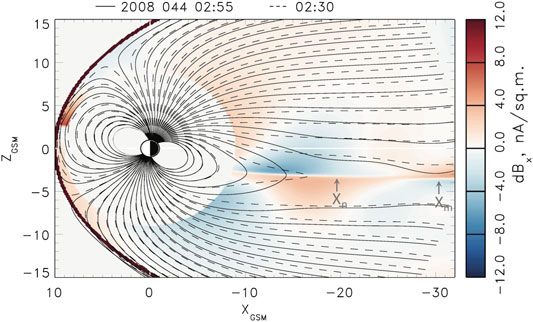
FIGURE 3. Color-coded variations of the x-component of the magnetic field between moments $t_0=02:30$ UT and $t_2=02:55$ UT $d{B}_x=B_x\left(t_2\right)-B_x\left(t_0\right)$ in the noon-midnight meridional plane with overplotted magnetic field lines (solid lines for the moment $t_2$ and dashed lines for the moment $t_0$) for the 13 February 2008 substorm. The approximate location of the X-lines $X_n$ and $X_m$ is marked by gray arrows. Magnetic field lines start from the ionosphere at ${60}^{\circ }$ with $2^{\circ }$ step in latitude. White disks $1R_E<r<9R_E$ in panels (B) and (C) mask magnetic field variations in the inner magnetosphere.

FIGURE 4

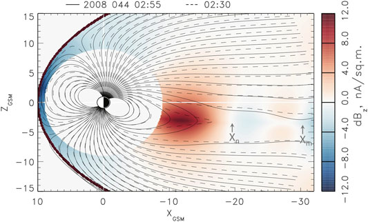
FIGURE 4. Color-coded variations of the z-component of the magnetic field between moments $t_0=02:30$ UT and $t_2=02:55$ UT $d{B}_z=B_z\left(t_2\right)-B_z\left(t_0\right)$ in the noon-midnight meridional plane with overplotted magnetic field lines in the format similar to Figure 3 in case of the 13 February 2008 substorm.

The difference in $d{B}_{x,z}$ values in regions $x\approx -20R_E$ and $x\approx -31R_E$ seen from Figures 3, 4 suggests that the reconnection process near $X_m$ is more steady-state than near $X_n$. The unsteady nature of the near-Earth reconnection is particularly well seen from $B_z$ variations earthward of $X_n$ in Figure 4. Moreover, the analysis of the equatorial $B_z\left(x\right)$ profiles with the 5-min cadence provided in Fig. 8i of [27] shows that the main part of the $B_z$ changes earthward of $X_n$ shown in Figure 4 occurs in the 5-min interval between $02:35$ UT and $02:40$ UT. Furthermore, the analysis of the magnetic flux redistribution in the lobes made in [27] gives an estimate of the average electric field in the steady-state reconnection region $E_y\sim 0.01v_A{B}_0/c$ for $B_0=40$ nT and $v_A=\mathrm{1,000}\mathrm{km}/\mathrm{s}$, consistent with the theoretical estimates that impose the upper limit for the reconnection rate $E_y/\left(v_A{B}_0/c\right)\sim 0.1$ [61, 62, and refs. therein] or $\approx 0.2$ [63]. Therefore, one can expect the reconnection near $X_m$ to be steady and its electric field homogeneous in space, whereas near $X_n$ to be more transient and structured. Below we show that a similar combination of steady and unsteady reconnection regions can be reproduced in PIC simulations of weakly driven magnetotail equilibria with some of the observed growth phase features.

4 6 August 2017 Substorm: Complex Reconnection Picture Resolved Using Advanced DM Method

In this section we consider another substorm event with a more complex structure of dipolarizations and X-lines. It occurred on 6 August 2017 and is also interesting because of a possible X-line crossing detected by the MMS mission. Its signatures were the $B_z$ reversal (Figure 5C), the ions bulk flow reversal and the large dawnward electron bulk flow velocity (not shown). At the same time, at the moment of the reversal the $\left|B_x\right|$ and $B_y$ magnetic field components were relatively large (Figures 5A,B) so that the total magnetic field exceeded 10 nT. We reconstruct this event using an advanced version of the KNN algorithm where the statistical weights of NNs depend on their proximity to the event of interest (e.g., [29]). In this algorithm, the model magnetic field $B^{\left(\mathrm{mod}\right)}$ is determined by minimizing the RMS of its deviation from observations $B^{\left(obs\right)}$

$M_{err}^{\left(NN\right)}=\sqrt{{\displaystyle \sum _{j\in S_{NN}}{\displaystyle \sum _{i=x,y,z}{w}_j{w}_{\left(0\right)}\left(r\right){\left[B_i^{\left(\mathrm{mod}\right)}\left(r^{\left(j\right)}\right)-B_i^{j,obs}\right]}^2}}},(9)$

where $S_{NN}$ is a set of $K_{NN}^{\left(B\right)}$ magnetometer measurements of the magnetic field components $B_i^{j,obs}$ with ephemeris $r^{\left(j\right)}$, corresponding to the selected set of $K_{NN}$ nearest neighbors; $w_{\left(0\right)}$ is the original weighting factor, which is a function of the real-space distance r from Earth, introduced in [44] to mitigate the spatial inhomogeneity of observations, especially at geosynchronous orbit. A distinctive feature of the weighted KNN algorithm is that each term in the sum in Eq. 9 has now an additional weighting factor

$w_j=\text{exp}\left[-{\left(R_q^{\left(j\right)}/\sigma R_{NN}\right)}^2/2\right],(10)$

FIGURE 5

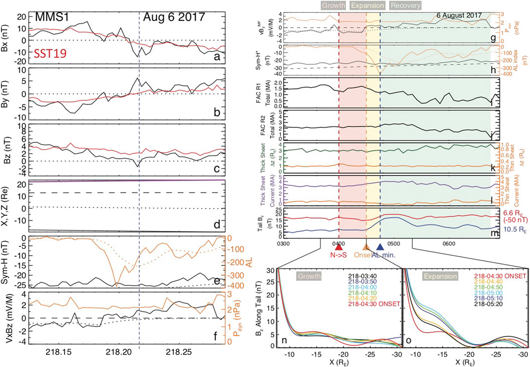
FIGURE 5. Validation results (using MMS1 data with 5-min cadence) and analysis of the 6 August 2017 substorm. Panels (A–C) show observed (black lines) and reconstructed (red lines) values of the GSM magnetic field components, (D) the MMS1 probe ephemeris (X, Y, Z and the radial distance R (black solid, dashed, dotted and purple lines, (E)$Sym-H^{\text{*}}$) (black line) and $AL$ (orange line) indices of storm and substorm activity, as well as (f) the solar wind electric field parameter $v{B}_z^{IMF}$ (black line) and solar wind dynamic pressure $P_{dyn}$ (orange line). Dotted lines in panels (E, F) show the smoothed values of indices and solar wind electric field corresponding to their DM input functions (2), (4) and (6). The moment of the possible X-line crossing is marked by the vertical dashed line. Panels (G) and (H) repeat the solar wind electric field and dynamic pressure parameters as well as geomagnetic indices (dotted lines show the corresponding smoothed values) to guide the analysis. (I, J) The square root of the sum of the squared amplitude coefficients for the high and low-altitude parts of the FAC modules, respectively (labeled here as FAC R1 and FAC R2). (K) The equatorial CS half thickness parameters D (green) and $D_{TCS}$ (orange). (L) The westward current from the thick CS module passing through the rectangle: $-16R_E\le X\le -6R_E$ and $-5R_E\le Z\le 5R_E$ (deep violet) and the westward current from the TCS module passing through the rectangle: $-16R_E\le X\le -6R_E$ and $-1R_E\le Z\le 1R_E$ (orange). (M) Total modeled $B_z$ field sampled at $r=\left(-6.6R_E,\mathrm{0,0}\right)$ in red and $r=\left(-10.5R_E,\mathrm{0,0}\right)$ in blue. (N, O) Total modeled $B_z$ sampled along the line $\left(-31R_E\le X\le -7.5R_E\right)$ during the growth and expansion phases, respectively. The moment of time, when each $B_z$-profile was sampled, is specified by the corresponding colored text in the format “DOY-hour-minute”.

Here $R_q^{\left(j\right)}$ is the distance (1) of the corresponding NN from the query point q and $R_{NN}$ is the radius of the sphere containing NNs in the binning space $\left(G_1,\dots ,G_5\right)$. When $\sigma \gg 1$, all distance-modulated weights $w_j\approx 1$ and NNs are not weighted. In contrast, for $\sigma <1$, the new weighs $w_j$ are well modulated within the sphere $R_q^{\left(j\right)}<R_{NN}$. This increases the statistical weight of measurements that were made at the more similar state and input conditions of the magnetosphere, according to the metric (1).

The weighted KNN approach is shown to result in better sensitivity of the model to variations of the magnetospheric state (e.g., storm or substorm phase) by using effectively much smaller numbers of NNs without overfitting [70]. Below we provide the DM reconstruction results with the parameters similar to those used in the previous section and with the weighting factor $\sigma =0.5$. Validation results for this event using the MMS1 probe data are presented in the left panels of Figure 5 and they show a reasonable agreement, especially for the $B_z$ component, where it does not exceed ∼2 nT.

The reconstruction summary for this substorm in the format used earlier in [26, 27] is presented in the right panels of Figure 5. Following [26], we consider the growth phase starting from the first point with $B_z^{IMF}<0$ in the 5-min cadence series (vertical red dashed line corresponding to t = 04:00 UT). The onset time 04:20 UT (vertical orange dashed line) is selected because of the strong change of the negative slope of the $AL\left(t\right)$. The start of the recovery phase (23:40 UT, vertical blue dashed line) corresponds to the minimum of the $AL$ index. The recovery phase is postulated to end when the AL > −25 nT, in accordance with [26, 27].

Figures 5H–J show weak storm activity: small and constant values of -$Sym-H^{\text{*}}$ and low-latitude field-aligned currents FAC R2. In the expansion phase (yellow zone) the amplitude of the TCS (Figure 5L) decreases, consistent with the earlier DM analyses [26, 27] (with small variations of the thickness parameters D and D_{TCS}, according to Figure 5K), while the equatorial magnetic field in the near-Earth tail (Figure 5M) increases making the magnetic field more dipole-like. At the substorm onset, the evolution of the equatorial magnetic field along the midnight meridian (red lines in Figures 5N, O) reveals wavy perturbations similar to the tearing mode (e.g., Fig. 6.2.9 in [71]). However, their wavelength is rather macroscopic, in contrast to the electron- or ion-scale tearing modes discussed earlier in theory and kinetic simulations of the magnetotail reconnection onset ([72, 73] and refs. therein). Further it results in the formation of new X-lines (Figure 5O) whose structure and evolution are better seen in Figures 6, 7.

FIGURE 6

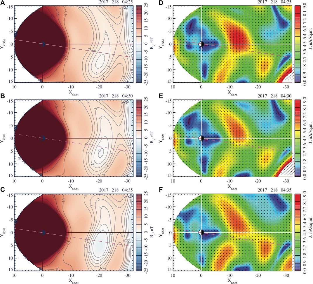
FIGURE 6. Distributions of the equatorial magnetic field $B_z$ [(A–C)] and the electric current [(D–F)] obtained using 0-degree tilt angle for the first dipolarization of the 6 August 2017 substorm. The arrows are vectors of the equatorial current density whose absolute value is color coded. The oblique dashed pink lines show the meridional planes, which are used below to investigate this dipolarization.

FIGURE 7

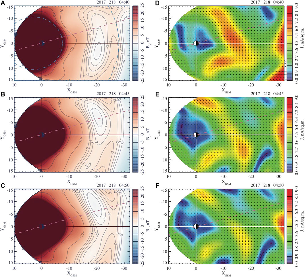
FIGURE 7. Distributions of the equatorial magnetic field $B_z$ [(A–C)] and the electric current [(D–F)] obtained using 0-degree tilt angle for the second dipolarization of the 6 August 2017 substorm. The format is similar to Figure 6. The oblique dashed pink lines show the meridional planes, which are used below to investigate this dipolarization. The dashed blue arcs in panel (A) show sample integration paths, which are used below to evaluate the closed magnetic flux evolution.

An interesting feature of this event is that the magnetic field dipolarization in the expansion phase has two sub-phases: 04:20–04:35 UT and 04:40–04:55 UT. Indeed, Figures 6, 7, which describe the evolution of the equatorial magnetic field and current, reveal two successive reconfigurations developing in the premidnight and postmidnight sectors. Figure 6 shows that during the first dipolarization a new X-line forms at $x\sim -20R_E$ along with the pre-exisitng X-line near $x\sim -30R_E$. As it is shown in Figure 8, the used NN subsets are sufficiently extended over the tail to resolve both X-lines. As is seen from Figures 6D–F, the equatorial current during this dipolarizaation becomes bifurcated.

FIGURE 8

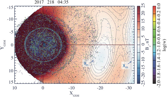
FIGURE 8. Two X-lines, $X_n$ and $X_m$ resolved in the equatorial distribution of the magnetic field $B_z$ (using 0-degree tilt angle) as earthward parts of the contours $B_z$ for the 6 August 2017 substorm. The format of this figure is similar to that of Figures 1B, 2. However, in contrast to Figure 2, the projections of the spacecraft coordinates on the equatorial plane are now shown by colored dots. The color of the jth dot reflects the distance $R_q^{\left(j\right)}$ of the corresponding NN from the query point $\text{log}{w}_j=-{\left(R_q^{\left(j\right)}/\sigma R_{NN}\right)}^2/2$, according to the weight definition (10).

The second dipolarization described in Figure 7 causes stronger and more global changes of the near-Earth magnetic field (regions $R\mathrm{\lesssim }15R_E$ in Figures 7A–C). It also causes not only the formation of new flux ropes in the postmidnight sector but the azimuthal extension of the region of the depressed or even reversed equatorial magnetic field. According to Figures 7D–F, this is accompanied by the reduction of the equatorial current density. To quantify these processes, we integrated the equatorial field $B_z$ over arcs similar to dashed blue lines in Figure 7A from the dawn to dusk magnetopause boundaries. Each arc represents a part of the circle with the center $\left(x,y\right)=\left(3R_E,0\right)$ (the shift is used to avoid integration over whole circles within the magnetopause). As was argued in [27], the distribution along the tail of the corresponding integral parameter $Int\left(B_z\right)={\displaystyle \int B_{z}ds}$ (where $ds$ is the arc length element) may be a good proxy of the magnetic flux evolution in the closed field line region of the magnetotail. The distributions of $Int\left(B_z\right)$ along the tail shown in Figure 9 as functions of the arc’s most tailward value of x indicate that the main flux redistribution in this substorm is provided by the second dipolarization. They also suggest that the main part of the near-Earth dipolarization is provided by the redistribution of magnetic flux in the closed field line region. Indeed, the area under these curves is now magnetic flux. According to Figure 9B, the increase in flux during the second dipolarization in the region $10-17R_E$ is roughly equivalent to the decrease in flux at $17-26R_E$. If the dipolarization were provided by an increase of the lobe field reconnection at $\mathrm{\gtrsim }30R_E$ that would be seen as a net increase of flux within $\sim 30R_E$.

FIGURE 9

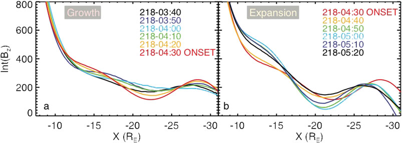
FIGURE 9. Analogs of Figs. 5n and 5o, now showing the line integral $Int\left(B_z\right)={\displaystyle \int B_{z}ds}$ over the arcs similar to dashed blue arcs in Figure 7A from dusk to dawn magnetopause boundaries (and expressed in units nT $R_E$) as a function of the arc’s most tailward value of x. The function $Int\left(B_z\right)$ better reflects the redistribution of the magnetic flux over the tail taking its width in the dawn-dusk direction into account.

To further investigate two dipolarizations occuring during this substorm, we present in Figures 10, 11 the meridional cuts of the cross current and in-plane magnetic field components $B_{x^{\prime },x^{″}}$ and $B_z$ in the planes marked by dashed lines in Figures 6, 7 (${x^{\prime }}_{GSM}$ and ${x^{″}}_{GSM}$ are the coordinates along the dashed lines in Figures 6, 7). These figures show processes similar to the 13 February 2008 dipolarization and shown in Figs. 12 and 13 in [27] as well as in Figures 3, 4. In particular, both dipolarizations reveal stronger variations of $d{B}_{x,x^{\prime }}$ and $B_z$ magnetic field components in the near-Earth reconnection region (around $X_n$) compared to the midtail one (around $X_m$). The differences between the magnetic field variations in Figures 10, 11 and those in Figures 3, 4, such as for instance, different relative phases of $d{B}_x$ and $d{B}_z$ variations can be explained by the larger time difference used in case of the 13 February substorm to calculate these variations. In fact, Figures 3, 4 describe the magnetic field variations during the 25-min long interval covering the whole expansion phase of that substorm, whereas Figures 10, 11 describe 15-min long partial dipolarizations that constitute the more complex tail reconfiguration during the 6 August 2017 substorm.

FIGURE 10

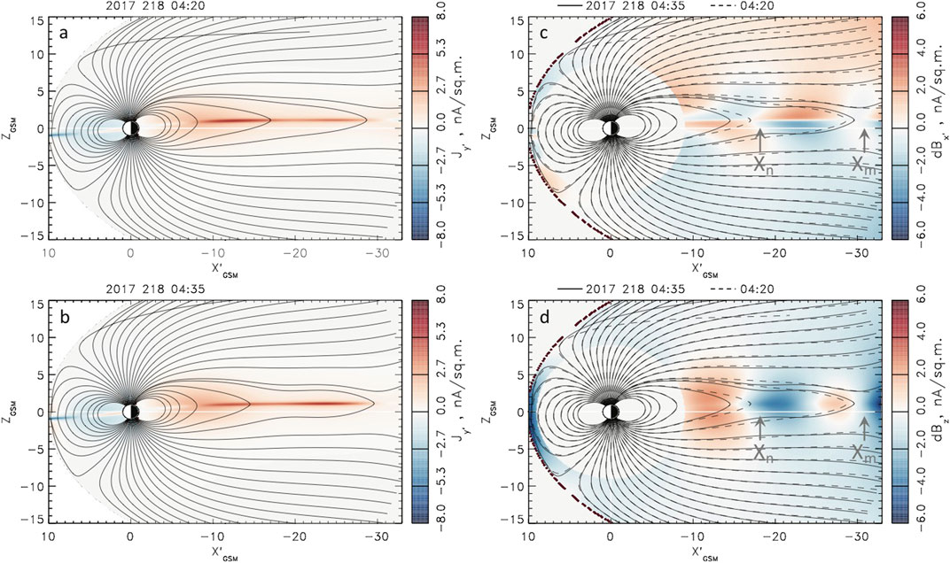
FIGURE 10. (A, B) Color-coded distributions of the current density component $J_{y^{\prime }}$ normal to the meridional plane shown by the dashed lines in Figure 6 with overplotted magnetic field lines (black solid lines) for the moments $t_0=04:20$ UT and $t_2=04:35$ UT of the first dipolarization during the 6 August 2017 substorm. (C, D) Color-coded distributions of the x’- and z-components of the magnetic field variation between moments $t_0=04:20$ UT and $t_2=04:35$ UT $d{B}_{x^{\prime },z}=B_{x^{\prime },z}\left(t_2\right)-B_{x^{\prime },z}\left(t_0\right)$ in the same meridional plane with overplotted magnetic field lines (solid lines for the moment $t_2$ and dashed lines for the moment $t_0$). ${x^{\prime }}_{GSM}$ is the coordinate along the dashed lines in Figure 6.

FIGURE 11

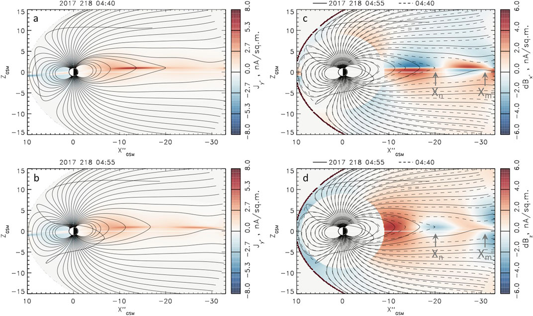
FIGURE 11. (A, B) Color-coded distributions of the current density component $J_{y^{″}}$ normal to the meridional plane shown by the dashed lines in Figure 7 with overplotted magnetic field lines (black solid lines) for the moments $t_0=04:40$ UT and $t_2=04:55$ UT of the second dipolarization during the 6 August 2017 substorm. (C, D) Color-coded distributions of the x”- and z-components of the magnetic field variation between moments $t_0=04:40$ UT and $t_2=04:55$ UT $d{B}_{x^{″},z}=B_{x^{″},z}\left(t_2\right)-B_{x^{″},z}\left(t_0\right)$ in the same meridional plane with overplotted magnetic field lines (solid lines for the moment $t_2$ and dashed lines for the moment $t_0$). ${x^{″}}_{GSM}$ is the coordinate along the dashed lines in Figure 7.

As one can seen from the comparisons of Figures 10A,B, the first dipolarization is relatively weak, and it does not cause any significant flux redistribution, according to Figure 9B. During the first dipolarization, the magnetic field variations near $X_n$ (Figures 10C,D) are confined to the region $x>-27R_E$ and $-2R_E\mathrm{\lesssim }z\mathrm{\lesssim }4R_E$. The near-Earth X-line during this dipolarization forms in the center of the TCS, which extends from $-28R_E$ to $-9R_E$ (Figure 10A). It only moderately redistributes its current density (Figure 10B).

In contrast, during the second dipolarization, the (already shorter, less than $\sim 10R_E$ in the radial extension) TCS disappears (Figures 11A,B), the near-Earth X-line forms at its tailward end and these processes are associated with a significant flux redistribution shown in Figure 9B (compare yellow and green curves).

It is important to note that these processes of the tail thinning and dipolarization often occur under weak variations of the lobe magnetic field. Its weak variations in the growth phase were reported in [74–76] and they are seen in Figure 10C as well as in [27] (Figs. 12, 16, S4 and S13). Even rapid dipolarization processes shown in Figures 4, 11C are accompanied by more gradual lobe field variations, consistent with other data analyses [58, 74].

5 Kinetic Simulations of Magnetotail Reconnection Guided by Empirical Reconstructions

In order to understand the physical mechanisms of the formation of several X-lines in the magnetotail and their different reconnection regimes revealed in the DM analysis, we performed PIC simulations of the tail current sheet equilibrium sharing some of the observed pre-onset tail features. In particular, the reconstruction of the February 13 event discussed above in ([27], Fig. 8h) suggests that the near-Earth reconnection is preceded by the formation of a flux accumulation region near $x\approx -22R_E$. According to Figure 6A, similar pre-onset features in the form of a wide valley with small $B_z$ values at $R\sim 22R_E$ and the enhanced $B_z$ ridge earthward of that valley took place prior to the 6 August 2017 substorm. To take these features into account, the PIC simulations start from a 2-D equilibrium with a $B_z$ hump described by the vector potential $A^{\left(0\right)}=\left[0,-\psi \left(x,z\right),0\right]$, where $\psi =L{B}_0\text{ln}\left(\beta \left(x\right)\text{cosh}\left\{z/\left[L\beta \left(x\right)\right]\right\}\right)$, L is the characteristic current sheet thickness parameter, and the x-axis points from Earth to Sun. Its variation along the tail is determined by the function $\beta \left(x\right)=\exp \left[{\epsilon }_{1}g\left(\xi \right)\right]$, with $\xi =x/L$, ${\epsilon }_1\ll 1$ and $-g\left(\xi \right)=\xi +\left(\alpha /{\epsilon }_2\right)\left\{1+\text{tanh}\left[{\epsilon }_2\left(\xi -{\xi }_0\right)\right]\right\}$, which provides a region of accumulated magnetic flux near $\xi ={\xi }_0$. This is seen from the magnetic field profile $B_z(x,z=0)={\epsilon }_1{B}_0\left\{1+\alpha {\text{cosh}}^{-2}\left[{\epsilon }_2\left(\xi -{\xi }_0\right)\right]\right\}$ having a characteristic hump. The corresponding class of isotropic plasma equilibria was first proposed in [77] based on the 2-D generalization [78] of the 1-D Harris model [79] to describe spontaneous onset of the ion tearing instability.

The PIC simulations were performed using an open boundary modification [64, 80] of the explicit massively parallel code P3D [81] in a 3-D box with dimensions $L_x^{\left(s\right)}\times L_y^{\left(s\right)}\times L_z^{\left(s\right)}=80d_i\times 5d_i\times 20d_i$, where $d_i=c/{\omega }_{pi}$ is the ion inertial scale and ${\omega }_{pi}={\left(4\pi e^2{n}_0/m_i\right)}^{1/2}$ is the plasma frequency; $n_0$ is the plasma number density at the earthward side of the simulation box near the neutral plane ($z=0$). The choice of such a relatively long in x and narrow in the y-direction box was motivated by the available computer resources and the necessity to cover a large portion of the tail containing both X-lines resolved by the DM method and described in the previous section. In particular, with d_i∼500 km$\sim 0.1R_E$ [82], the distance between X-lines in our run is $30d_i\sim 3R_E$, that is only 3–4 times smaller than in the DM reconstruction. At the same time, our previous simulations of similar equilibria with shorter in x and wider in y boxes, up to $L_y^{\left(s\right)}=20d_i$ (see, for instance, Fig. 13 in [82]) suggest that the selected value of $L_y=5d_i$ with periodic boundaries in the y-direction is sufficient to reproduce major structuring in that direction, including ballooning/interchange and flapping motions.

The plasma parameters include the mass ratio $m_i/m_e=128$, ion-to-electron temperature ratio $T_i/T_e=3$ and the effective Alfvén speed $v_A=B_0/\sqrt{4\pi n_0{m}_i}=c/15$ where c is the speed of light. The equilibrium magnetic field parameters are ${\epsilon }_1=0.03$, ${\epsilon }_2=0.2$, $\alpha =3$, and ${\xi }_0=-30$ with the CS thickness parameter $L=1d_i$. The magnetic and electric fields are normalized, respectively, by $B_0$ and $v_A{B}_0/c$. The coordinates are normalized by $d_i$ and velocity components by $v_A$. The simulation grid has $2560\times 160\times 640$ cells with $\approx 230$ particles per cell corresponding to $n=n_0$. The magnetic field configuration at the early stage of the run is shown in Figure 12A.

FIGURE 12

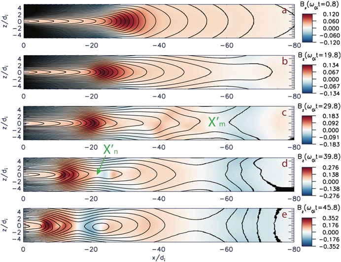
FIGURE 12. (A) The initial magnetic field configuration in PIC simulations of magnetotail reconnection, which is shown here as a color-coded distribution of the $B_z$ component with overplotted magnetic field lines in the plane $y=2.5d_i$ (“2D-equivalent” field lines calculated by treating a slice of the 3-D domain as if it were a 2-D simulation). (B–E) magnetic field distributions at later moments showing (B) the CS thinning, (C) the formation of the “mid-tail” X-line $X_m$′, (D) another “near-Earth” X-line $X_n$′ near $x=-20d_i$, (E) the fully developed tail reconnection picture at the moment, which is further explored in more detail.

In contrast to earlier simulations ([83], and refs. therein) that described spontaneous onset regimes, here we drive the system by imposing a weak external electric field $E_y^{\left(dr\right)}$ at top and bottom boundaries. This setup resembles earlier simulations of the externally driven electron tearing [73], and the whole setup is therefore a combination of the earlier ion and electron tearing modeling efforts. Still, in contrast to earlier setups with localized in x driving fields [73, 84, 85] and similar to [64], we do not assume any localization of the driving electric field along the tail. It remains constant throughout the main part of the box length $L_x$, being only attenuated near open boundaries. For example near the left boundary $E_y^{\left(dr\right)}=E_0{\left[\text{tanh}\left(x-\delta \right)/\delta \right]}^2$ with $\delta =0.1L_x$. The actual structure of the driving electric field remains insufficiently resolved in observations and it can only be conjectured from global MHD simulations (e.g. [86]). In this situation, the assumption of the homogeneous electric field appears to be the most plausible ad hoc assumption. The driving field amplitude $E_0$ smoothly increases in a half of the ion gyrotime $1/{\omega }_{0i}$ at the beginning of the run and then remains constant with $E_0=0.05$.

The external driving first results in the CS thinning and stretching, which are seen particularly well in the tailward part of the box (Figure 12B). It also causes the buildup of the plasma pressure in the region $x\mathrm{\lesssim }-24d_i$ (not shown), consistent with previous studies of the driven reconnection regimes (e.g., Fig. 9 in [73]). This makes the CS configuration more similar to empirical reconstructions with extended TCS, such as for instance in Figures 10A, 11A (see also [27], Figs. 12b). At some point, the first X-line ${X^{\prime }}_m$ forms in the “tailward” part of the simulation box (Figure 12C). However, the second X-line ${X^{\prime }}_n$ forming later in the left (“earthward”) part of the box (Figure 12D) is not the secondary X-line caused by the tearing instability of the reconnection exhausts (e.g. [87]), because it also forms in the absence of any primary X-lines [88–90] or when the primary X-line shows no reconnection signatures [72, 82]. ${X^{\prime }}_n$ rather forms because of the flux starvation effect created by the earthward-moving DF in its trailing part. As it was shown in [72, 88, 89], the DF appears from the original $B_z$ hump due to its spontaneous acceleration and further localization in x.

It is very interesting that the magnetic field perturbations shown in Figure 12E strongly resemble the DM reconstructions of substorm dipolarizations shown in Figures 4, 10D, 11D with much stronger bipolar $B_z$ perturbations around the near-Earth X-line compared to the midtail region. This suggests that reconnection near ${X^{\prime }}_n$ is unsteady, in contrast to the steady midtail reconnection process at ${X^{\prime }}_m$. This conclusion is further confirmed in our simulations by the analysis of the electric field and plasma parameters.

Figure 13A shows that the electric field distributions around the X-lines are indeed drastically different. Around ${X^{\prime }}_m$ ($x\sim -50d_i$) the distribution of $E_y\left(x,z\right)$ is homogeneous and its value $E_y\left(x,z\right)\approx 0.1$ is consistent with the theoretical estimates [61–63]. These are strong indications of the steady reconnection process. In particular, the broad distribution of the electric field $E_y$ over a large area in the plane $\left(x,z\right)$ justifies the concept of the reconnection rate, measured by $E_y$, as a global parameter, which characterizes the reconnection process as a whole. In contrast, near ${X^{\prime }}_n$ ($x\sim -15d_i$) the reconnection electric field strongly varies in space. However, not all these variations are related to unsteady reconnection. In particular, the sign-alternating variations of $E_y$ near the O-line ($x\sim -23d_i$) describe north-south flapping motions of the CS as a whole, which are also seen in Figure 13F as strong variations of the magnetic field $B_x$ ($\sim 0.5B_0$) without noticeable $B_z$ variations in the same region (Figure 13G). The properties of non-reconnection flapping and ballooning/interchange motions (seen in the region $x\sim -5d_i$ in Figure 13G) in this run with a relatively small extension in the y-direction are similar to non-reconnection motions investigated with larger in y boxes in PIC simulations of spontaneous reconnection onset regimes [82], where they are compared with the corresponding magnetotail observations and other kinetic simulations.

FIGURE 13

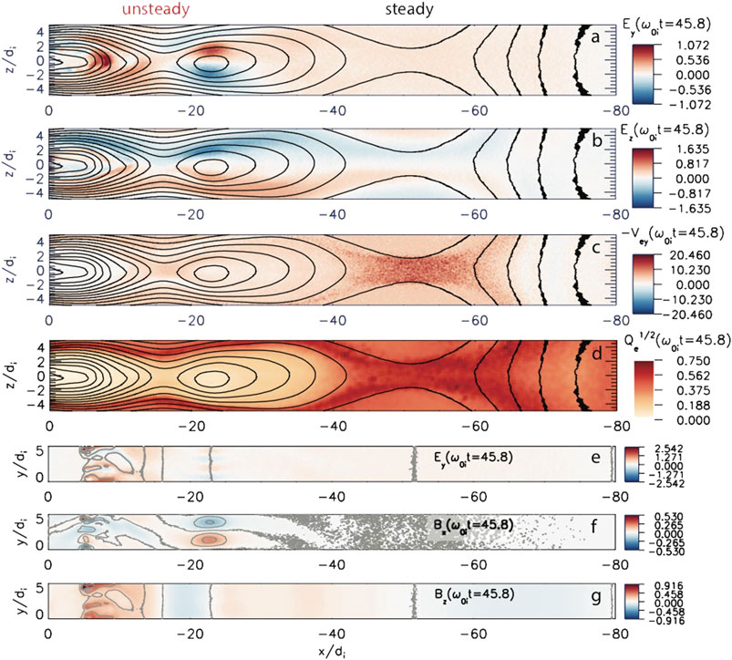
FIGURE 13. Steady and unsteady reconnection regions in weakly driven magnetoatail at the moment ${\omega }_{0i}t=45.8$ corresponding to Figure 12E. (A–D) The distributions in the plane $y=2.5d_i$ of the electric field components $E_y$ and $E_z$, the electron bulk flow velocity $=-V_{ey}$ and the electron agyrotropy parameter $\sqrt{Q_e}$ [91] marking the localization of the electron diffusion region (in the latter case, to reduce noise in simulation outputs, the original numerical distributions are averaged over $20\times 20$ grid cells). (E–G) The distributions of the electric field $E_y$ and the magnetic field components $B_x$ and $B_z$ in the neutral plane $z=0$.

At the same time, earthward of $X_n\prime$ and near the DF, the electric field is structured in the y-direction due to ballooning/interchange perturbations that are best seen in variations of the magnetic field $B_z$ (Figure 13G). All in all, the electric field associated with the earthward motion of the DF is highly localized near its $B_z$ peak and its value strongly exceeds the steady-state reconnection limit 0.2 [63]. Note, that such strong values of the reconnection electric field were reported before in simulations of the ion tearing instability ([82], Fig. 5) and interchange-driven reconnection ([92], Fig. 11). Thus, the kinetic reconnection picture in our PIC simulation, which combines steady and unsteady reconnection regions, is quite consistent with the empirical DM-based reconstructions described in the previous section. Moreover, kinetic simulations reveal its features that cannot be captured from the empirical geomagnetic field analysis, because they represent spontaneous or small-scale plasma modes or they are not reflected in the magnetic field data at all. The examples of the first group of such phenomena are flapping and ballooning/interchange motions seen in Figures 13A,B. They are indeed observed in the tail [93–97], although their relation to substorms and their reconnection modes remains a topic of ongoing discussions [98]. Another example is DFs, with their ion-scale leading edges and fast ($v_x\sim v_A$) earthward propagation (e.g. [93]), forming out of relatively stationary and macroscopic $B_z$-humps (compare, for instance, Figures 12A,E).

In Figures 13B–D we present another group of signatures, which cannot be resolved using the DM analysis. Figure 13B shows the electric field directed toward the neutral plane $z=0$ and arising in ion and sub-ion-scale TCS due to different motions of electrons and ions on those scales [85, 99–102]. Similar effects of the electric field directed toward a negatively charged TCS were shown in PIC simulations ([101], Fig. 8) and in observations ([23], Fig. 9). Figures 13C,D show plasma signatures that are usually associated with the electron diffusion region (EDR) in steady reconnection regimes: The first shows super-Alfvénic dawnward electron flows [103] that have been found one of the key distinctive EDR features in recent MMS observations of the magnetotail reconnection [104]. The second reveals non-gyrotropic electron motions that are quantified using the agyrotropy parameter $\sqrt{Q_e}$ proposed by [91] and shown later in MMS observations as a distinctive EDR signature [105].

Finally, in Figure 14 we present the kinetic dissipation parameters for the unsteady part of this run and compare them with similar parameters inferred from MMS observations. In contrast to the steady-state reconnection area near ${X^{\prime }}_m$, the unsteady reconnection region near $X_n^{\prime }$ does not reveal impressive EDR signatures, such as the super-Alfvénic dawnward electron flows or the agyrotropy enhancement (left parts of Figures 4B,C). This is because the main process in this region is the formation and fast earthward movement of a DF and the resulting dipolarization of the magnetic field configuration [72, 88, 89]. Moreover, many key aspects of these processes can be described by ideal MHD models [106, 107], whereas the DF formation and acceleration processes are shown to resemble the ion tearing instability [64, 72] supported by the ion Landau dissipation [108]. However, quantifying the latter in simulations and observations is a challenging problem because the conventional single-fluid measure, the Joule heating rate cannot distinguish between ion and electron Landau dissipation in collisionless magnetospheric plasmas. Indeed, the energy conversion rates in the frame moving with ions or electrons $j\cdot {{\mathrm{E}}^{\prime }}_{\mathit{e,i}}$ (where $j=j_i+j_e$, ${{\mathrm{E}}^{\prime }}_{\mathit{e,i}}=E+v_{e,i}\times B/c$, $j_{e,i}$ are the electron/ion currents in the laboratory frame of reference and $v_e$ and $v_i$ are the electron and ion bulk flow velocities) are same for ion and electron species $j\cdot {{\mathrm{E}}^{\prime }}_{\mathit{e}}\approx j\cdot {{\mathrm{E}}^{\prime }}_{\mathit{i}}$ assuming plasma quasi-neutrality $n_e\approx n_i$).

FIGURE 14

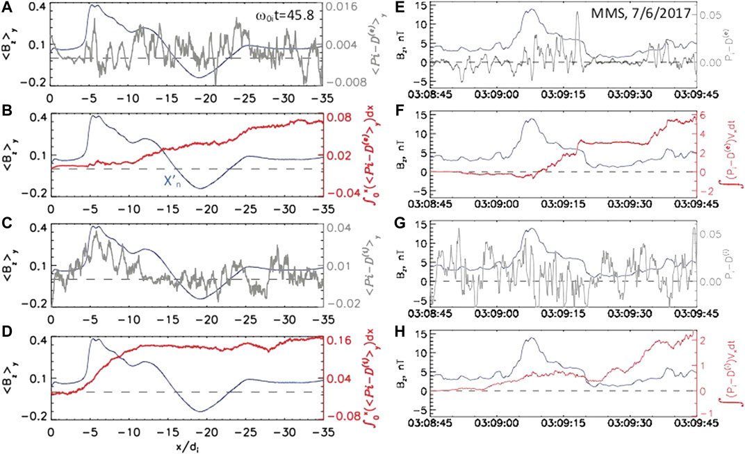
FIGURE 14. (A–D) Kinetic dissipation parameters in the unsteady reconnection region in PIC simulations (Figure 13) and (E–F) similar parameters derived from MMS observations of a DF on 6 July 2017 at $\left(x,y,z\right)=\left(-\mathrm{19,3,3}\right)R_E$. From top to bottom the panels show the profiles of averages ${\langle \dots \rangle }_y$ over the y direction $0<y<5d_i$ for (A) the electron dissipation parameter ${\langle Pi-D^{\left(e\right)}\rangle }_y$ (gray line), (B) its value integrated in x: ${\displaystyle {\int }_0^x{\langle Pi-D^{\left(e\right)}\rangle }_{y}dx}$ (red line), (C) the ion dissipation parameter ${\langle Pi-D^{\left(i\right)}\rangle }_y$ (gray line), (D) its value integrated in x: ${{\displaystyle {\int }_0^x\langle Pi-D^{\left(i\right)}\rangle }}_{y}dx$ (red line) at the moment ${\omega }_{0i}t=45.8$, which is also described in Figures 12E, 13. In all panels the magnetic field $B_z$ profile is shown by blue lines. Panels (G–M) show parameters similar to (A–F) as functions of time in MMS observations in the format (hour:min:sec).

To solve this problem, it has recently been proposed [109] to employ the new kinetic parameter $Pi-D^{\left(\alpha \right)}=-{\text{Π}}_{ij}^{\left(\alpha \right)}{D}_{ij}^{\left(\alpha \right)}$ ($\alpha =e,i$), the double contraction of deviatoric pressure tensor ${\text{Π}}_{ij}^{\left(\alpha \right)}=p_{ij}^{\left(\alpha \right)}-{\delta }_{ij}{p}^{\left(\alpha \right)}$ (where $p^{\left(\alpha \right)}=p_{ii}^{\left(\alpha \right)}/3$) and traceless strain-rate tensor $D_{ij}^{\left(\alpha \right)}=\left({\partial }_i{v}_j^{\left(\alpha \right)}+{\partial }_j{v}_i^{\left(\alpha \right)}\right)/2-{\delta }_{ij}{\theta }^{\left(\alpha \right)}/3$ (with ${\theta }^{\left(\alpha \right)}=\nabla \cdot v^{\left(\alpha \right)}$), which was introduced earlier in [110]. It was demonstrated [109] that the $Pi-D$ parameters represent direct analogs of the MHD Joule heating as an entropy variation measure and that they have different distributions for electrons and ions. It was shown that in the regions with ion $Pi-D^{\left(i\right)}$ peaks, at the leading part of the DF, ion distributions show signatures of multi-flow motion, including ions reflected from the DF. Such multi-flow ion motions have indeed been detected at DFs in Cluster, THEMIS, and MMS observations [111–114].

In Figures 14A–D we present kinetic dissipation measures obtained in PIC simulations and averaged over the y direction $0<y<5d_i$, along with the corresponding profile of the magnetic field $B_z$ shown here to provide the global context for this local investigation. As one can see from Figures 14A,B, while the linear distribution of the electron dissipation parameter ${\langle Pi-D^{\left(e\right)}\rangle }_y$ remains irregular and not obviously positive, its integration along the tail reveals its persistent accumulation upstream of the DF structure (red line in Figure 14B). The increase starts from the ${X^{\prime }}_n$ vicinity with another buildup near the corresponding O-line. The ion dissipation parameter is even more impressive: Already its average over the y-coordinate reveals a peak near the DF (Figure 14C), and when integrated along the tail ${\displaystyle {\int }_0^x{\langle Pi-D^{\left(i\right)}\rangle }_y}dx$ builds up near the DF and remains elevated farther in the tail (red line in Figure 14D).

Figures 14E–H show the dissipation parameters similar to those in Figures 14A–D but now derived from MMS observations of a DF on 6 July 2017, a relatively rare case of a slow moving DF with the ion bulk flow speed smaller than 200 km/s. The four-probe sub-ion-scale MMS observations of the electromagnetic field and plasma parameters provide the unique opportunity to measure the kinetic dissipation parameters $Pi-D$ for both electrons and ions. At the same time, even with the MMS capability of calculating higher moments of the plasma distribution, the assessment of the kinetic dissipation parameters remains a challenging problem. In particular, even in the MMS burst mode with the sampling time $\delta t=0.15\mathrm{s}$ [115] and probe spacing $\delta r\mathrm{\lesssim }20\mathrm{km}$, any velocity gradient estimates necessary for calculation of the tensor $D_{ij}^{\left(i\right)}$ may give trivial results for structures moving much faster than $V_{max}=\delta r/\delta t\approx 133\mathrm{km}/\mathrm{s}$. Thus, MMS data is only appropriate so far to study the kinetic dissipation in relatively slow moving DFs.

In spite of these caveats, simulation and observation results presented in Figure 14 have interesting similarities. In particular, both simulations and data show the accumulation of positive $Pi-D$ values for electrons after integration (over x in simulations and in time in observations) seen in Figures 14B–G. Both in simulations and in observations (Figures 14B,F) the electron dissipation builds up behind the DF, upstream of the ion dissipation buildup, in the regions with relatively small values of the magnetic field, while for ions the dissipation starts accumulating at or even before the DF.

6 Discussion

6.1 Error Analysis of Empirical Reconstructions

In this study we provided a DM reconstruction of magnetic reconnection in the Earth’s magnetotail associated with its dipolarizations during substorms. A direct validation of this reconstruction can only be provided using a limited number of in-situ observations available at the moment of interest. This is an unavoidable feature of the DM method as a data discovery tool, which extracts from data the information (e.g., on the global structure of the magnetotail), which cannot be obtained by other methods. We simply have no real constellations of $\sim 3\cdot {10}^4$ probes to comprehensively validate our results. Still, the 13 February 2008 substorms were validated by all five THEMIS probes (Figs. S6–S7 in [27]), while for the 6 August 2017 event, the MMS1 validation results are presented in Figure 5. Moreover, the uncertainty of the DM method caused by averaging over the NN bins can be quantified by comparing the original values of the parameters $G_1$-$G_5$ with their NN means. For the 13 February 2008 reconstruction such information was provided in Fig. 19 of [27]. For the 6 August 2017 substorm we provide it in Figure 15. This figure shows in particular that during the dipolarization intervals considered in Section 4 and shown by vertical dashed lines, the maximum deviation of the binning parameters averaged over their NN bins from their original values defined by Eqs. 4–6 does not exceed ∼10% (the largest deviation is seen for $\langle AL|$ at the end of the second dipolarization interval). This means that statistical errors of the presented reconstruction of the magnetic field during this substorm are much smaller compared to major variations of the binning parameters. Therefore the presented DM-based picture of magnetotail reconfigurations should indeed reflect the characteristic features of magnetic reconnection during substorms.

FIGURE 15

FIGURE 15. The substorm part of the binning parameters (4)–(6) $\langle AL|$, $D\langle AL|/Dt$ and $\langle {\text{vB}}_s^{\text{IMF}}|$ (blue lines) and their means over $\mathrm{32,000}$ NN bins (${\{\dots \}}_{NN}$, red lines) for the 6 August 2017 substorm. Parameters $\langle AL|$ and $D\langle AL|/Dt$ are normalized by the corresponding unit convolution integrals $\langle 1|$. Vertical dashed lines mark two dipolarization intervals considered in Section 4.

Consistent with the analysis of the 13 February 2008 substorms [27], we have found that the relatively strong deviations of the binning parameters from their means over NNs take place for the solar wind parameter $\langle {\text{vB}}_s^{\text{IMF}}|$ and the $AL$ index in the recovery phase. This suggests that the solar wind and the magnetosphere after substorms are less coherent (perhaps turbulent) and hence less reproducible, compared to the evolution of the magnetosphere during growth and expansion phases.

An important source of uncertainty in the present NN approach may be the instrument errors and combining probes from different epochs. Fortunately, the accuracy of magnetic field measurements critical for our investigation (with a few nT accuracy necessary to resolve the $B_z$ magnetic field in the tail) was sufficiently high. In particular, the IMP8 magnetometer was good to 0.3 nT [116] and later missions had largely better instruments (e.g. [117–119]) with a few caveats. Significant errors (up to 7 nT) were found for some geosynchronous missions [120] and they were mitigated using inter-spacecraft calibration. The errors in the external magnetic field (difference between the measured and dipole magnetic field values) may also be large in the inner magnetosphere because of the spacecraft attitude uncertainty and large values of the dipole field there [121]. However, this is not an issue in the magnetotail.

6.2 Implications for Local Reconnection Models and Tearing Stability

The concept of magnetic reconnection was introduced to explain explosive energy release and rapid changes of magnetic field topology associated with solar flares [2, 3], magnetospheric substorms [7, 108, 122] and laboratory current disruptions ([123], and refs. therein). But its theory turned out to be built mainly on models of steady-state reconnection regimes ([63, 124–127], and refs. therein). The few exceptions include the tearing instability theory [87, 108, 122, 128], and catastrophe models of coronal mass ejections and solar flares [129, 130].

At the same time, the description of transition from the slow evolution of the tail to its rapid reconfiguration has long been complicated by the almost universal tearing stability of the tail current sheet provided by magnetization of electrons due to nonzero northward magnetic field $B_z$ [131, 132]. As a result, the tail can be unstable when electrons become unmagnetized, under the condition $B_z/B_0\mathrm{\lesssim }k{\rho }_{0e}$, where $B_0$ is the field outside CS, k is the wave vector and ${\rho }_{0e}$ is the thermal electron gyroradius in the field $B_0$ [73, 122, 133]. The resulting electron tearing instability is enabled by the free energy of the mutual attraction of the parallel electric current filaments and the electron Landau dissipation of unmagnetized electrons. In PIC simulations, the corresponding electron-demagnetization mediated reconnection (EDMR) onset used to be reproduced due to stretching and thinning of a CS by the external electric field [73, 101, 134]. It is important that after the electron tearing instability phase (or in its absence in simulations with spatially localized driving [84, 85]) the reconnection process becomes quasi-steady ([83], and refs. therein), consistent with regimes found earlier in kinetic simulations with non-self-consistent setups using 1-D CS equilibria with an imposed X-line perturbation ([127], and refs. therein).

In 1974 Schindler [108] hypothesized that the tail could become unstable even with magnetized electrons if the CS is sufficiently thin to demagnetize ions and provide their Landau dissipation. The corresponding tearing instability must be much faster compared to the electron tearing. However, later it was found [135] that magnetized electrons change the free energy of the tearing mode, and eventually Lembege and Pellat [131] showed that the corresponding sufficient stability condition coincides with the Wentzel–Kramers–Brillouin (WKB) approximation $\pi \left(B_z/B_0\right)\mathrm{\lesssim }k{L}_z$, which allows one to consider stability neglecting the CS variations along the tail with the scale $L_x\sim L_z\left(B_0/B_z\right)$ ($L_z$ is the CS half-thickness) making the ion tearing impossible.

A missing key for ion tearing destabilization was found relatively recently when it was discovered [77] that the stability condition derived by Lembege and Pellat [131] is only valid for constant $B_z$ values. If $B_z$ changes along the tail, the stability condition takes the form $\pi \left(B_z/B_0\right)C_d^2\mathrm{\lesssim }k{L}_z$, where the parameter $C_d=V{B}_z/\left(\pi L_z\right)$ is determined by the flux tube volume per unit magnetic flux $V={\displaystyle \int dl/B}$. In particular, in the presence of a flux accumulation area with the tailward gradient of $B_z$, the parameter $C_d>1$ and a room for instability arises. The corresponding instability had indeed been found in PIC simulations with ad hoc configurations having $B_z\left(x\right)$ profiles with a hump [72, 88, 89]. Since electrons remained initially magnetized by the field $B_z$, the instability was essentially the ion tearing. It first led to the formation of an earthward-moving dipolarization front (DF), in whose wake new X-lines formed due to the flux starvation process [89]. The resulting ion-demagnetization dominated reconnection (IDMR) onset did not require any external driving and could be considered as spontaneous or “internally driven” by the DF formation and evolution processes.

Despite this clarity in the tearing stability theory and consistent simulation results, until now, the role of EDMR and IDMR regimes in the actual magnetotail dynamics remained unclear. In particular, it is unknown if/when the driving (ultimately due to the solar wind) is sufficiently strong to squeeze the CS down to electron scales and to provide EDMR with the subsequent steady reconnection, and when (if any) $B_z$ humps form to provide IDMR.

The present study provides interesting implications for the magnetotail stability and reconnection onset mechanisms. Our DM reconstructions suggest that both steady and unsteady reconnection regimes are possible in the magnetotail during substorms. At the same time, our PIC simulations guided by empirical reconstructions suggest that both IDMR and EDMR regimes are possible in the tail. Moreover, the former resembles the unsteady reconnection, while the latter becomes eventually steady, consistent with the classical fast and steady reconnection models ([62] and refs. therein).

6.3 Role of Thin Current Sheets

The use in Section 5 of isotropic plasma equilibria with shifted Maxwellian distributions for ions and electrons, inherited from the 1962 Harris solution [79], to explain the reconnection features found in our DM reconstructions may be questioned in view of another discovery in the DM analysis of substorms, namely the buildup of extended TCSs in the substorm growth phase and their decay in the expansion phase [26, 27] (see also Figures 10A,B, 11A,B of the present study).

The analysis of 2-D isotropic equilibrium models [136] suggests that they require strongly stretched magnetic field configurations (with sufficiently large values of the ratio $B_0/B_z$) to explain the formation of the ion-scale TCS sufficiently far from the Earth. Large values of $B_0/B_z$ are required to maintain the force balance between the magnetic field line tension and the pressure gradient $1/L_x\sim \left(B_z/B_0\right)/L_z$, where $L_x$ is the inhomogeneity scale of the TCS, $L_z$ is its half-thickness and $B_0$ is the lobe field [137]. Modeling TCSs with $L_x\gg L_z\left(B_0/B_z\right)$ might require more sophisticated equilibria with anisotropic and agyrotropic particle distributions (e.g. [136], and refs. therein).

Indeed, three of four substorm events on 13 February 2008 considered in [27] had relatively small values of $B_0/B_z\sim 10$ (according to their Figs. 15b–15d), whereas their aspect ratios $L_x/L_z$ often exceeded 50 (Fig. 16 in [27]). That finding was consistent with signatures of the multiscale structure of the magnetotail inferred from local observations of the pre-onset CSs [19, 20, 23, 51].

However, this is not the case for the event considered in Section 3, whose specific features (the $B_z$ hump and the ion-scale TCS earthward of it) guided our PIC simulations. In that first substorm of the 13 February 2008 series, the ratio $B_0/B_z$ reaches 70 in the late growth phase (yellow line in Fig. 15a, corresponding to 02:25 UT). Thus, the specific substorm event, considered in Section 3 of our DM analysis is close to the isotropic force balance state and it can be consistently described by 2-D isotropic CS equilibrium models of the class [78]. Moreover, the specific parameters used in our simulations correspond to $L_x/L_z\sim B_0/B_z\approx 33$ and $D_{TCS}\sim 0.1R_E$ and they are quite close to similar TCS parameters of the first substorm in the 13 February 2008 series in its late growth phase (02:25 UT): $L_x/L_z\sim 25$, $B_0/B_z=20-70$ and $L_z=0.2R_E$.

One can also provide more general arguments why the isotropic 2-D models can still be used in the local stability analysis of the realistic magnetotail. First, statistical studies show that the tail plasmas away from the dipole region are weakly anisotropic [138, 139]. At the same time, the DM reconstructions demonstrate that the current of the embedded TCS in the late growth phase may be small, compared to the total current, as is seen, for instance, from Figure 5L (this is the case for all four 13 February 2008 events as is seen from Fig. 8f in [27]). This suggests that the embedded TCS features and underlying non-isotropic plasma properties may only serve to provide the formation of the ion-scale TCSs sufficiently far from Earth, where their local stability properties can still be realistically reproduced by PIC simulations with isotropic equilibria and open x-boundaries. This is consistent with the results of statistical studies based on Geotail data [140], which suggest that the near-Earth X-line mainly forms near the tailward edge of the TCS. This appears to be the case during the second dipolarization in the 6 August 2017 event (Figure 11), although this is likely not the case during the first dipolarization when the near-Earth X-line forms in the middle of a very long TCS (Figure 10). Besides, even if the initial TCS is relatively short because of the corresponding force balance, the simulations performed in Section 5 suggest that it becomes more stretched and closer to empirical TCS reconstructions due to the external driving. To conclude, while some substorm dipolarizations certainly require a generalization of the isotropic plasma approximation, as it was outlined in [136], others can still be described using the conventional class of isotropic CS models [78, 79].

7 Conclusion

In this study, we investigated for the first time the magnetotail reconnection picture using modern data-mining methods, which allow us to employ for the reconstruction not only the magnetic field measurements available at the moment of interest but also other events in the historical database when the magnetosphere was in similar global states (substorm phases). The DM reconstruction revealed two distinctly different regions of magnetic reconnection with weak and strong changes of the magnetic field geometry. For both the 13 February 2008 and the 6 August 2017 substorms considered in our study the near-Earth X-line appears near $x=-20R_E$ at the substorm onset, which is defined in our work as a transition to the $AL\left(t\right)$ index evolution with a strong negative slope (dashed vertical orange line in Figure 5G–M). This result is consistent with the original conjecture of Hones [7], later single- and multi-probe studies of the near-Earth X-lines [57, 58], as well as with the plasmoid statistics [141]. In both events, the near-Earth X-line first appears in the pre-midnight sector (Figures 2, 6B), which is consistent with the earlier statistical investigations using Geotail [142] and Cluster [143] data.

In addition to earlier investigations, our DM reconstruction reveals that the near-Earth X-line ($X_n$) often co-exists with another more distant midtail X-line ($X_m$) located at $x\approx -30R_E$. In spite of the fact that its location is near the edge of the main cloud of historical magnetometer measurements [44], the analysis of data in the corresponding NN bins (Figures 2, 8) shows that the selected NN subsets provide sufficiently broad radial coverage of data to resolve both X-lines. The finding of the midtail X-line is consistent with another group of earlier observations suggesting persistent reconnection in the midtail around $30R_E$, which was inferred from THEMIS and ARTEMIS statistics of traveling compression regions [59, 60]. However, the coexistence of near-Earth and midtail X-lines has never been demonstrated before.

Moreover, the DM analysis shows that reconnection regimes at near-Earth and midtail X-lines are different. The near-Earth X-line appears at the substorm onset and then disappears from that region or reappears in another near-Earth region, e.g., in the postmidnight sector (compare Figures 7A,B or Figures 2, 10 in [27]). In contrast, the midtail X-line, after its appearance within the reconstruction validity region (here $R<32R_E$) in the late growth phase remains relatively stable and only gradually approaching the Earth (Figures 6A–C, 7A–C). Furthermore, the analysis of the magnetic field changes in the meridional plane (Figures 3, 4), which according to the Faraday’s law 8) quantifies the steadiness of the reconnection process, suggests that the latter is relatively steady near $X_m$ and transient at $X_n$.

To understand the physical mechanisms of the formation of several X-lines in the magnetotail and their different reconnection regimes, we performed 3-D PIC simulations of a relatively long ($L_x=80d_i$) tail CS region with open boundaries in the Sun-Earth direction. A new aspect of simulations was the combination of the initial TCS configuration having a region of the flux accumulation ($B_z$ hump) with a relatively weak and homogeneous external driving. The formation of the flux accumulation regions prior to unsteady reconnection in the near-Earth tail is found in the DM reconstruction of both substorm events (Fig. 8h in [27], as well as Figures 6A, 7A), consistent with earlier statistical results [144, 145]. Recently, it has been inferred from remote-sensing observations of 30–100 keV energy electrons precipitating from the tail CS during the substorm growth phase [146]. This feature is also interesting because the corresponding region with the tailward $B_z$ gradient (earthward of the $B_z$ hump) has been found in the tail stability theory [77] to be the only mechanism of destabilization of the ion tearing mode [108]. The second feature, the external driving was used before to reproduce the tail reconnection onset through the electron tearing instability [73]. It was also used in forced reconnection models [84, 85].

The reconnection picture in PIC simulations, guided by the DM reconstructions, is found to be surprisingly consistent with the empirical picture of the magnetotail reconnection. It also reveals two reconnection areas with distinctly different reconnection regimes, whose steadiness can now be checked using the explicit distributions of the electric field in the meridional plane (Figure 13A). It is found that farther in the tail, the reconnection process is steady and it reveals many signatures of the sustained collisionless reconnection process with the region of agyrotropic electron motion in its center. The corresponding dusk component of the electric field is broadly distributed in the meridional plane and hence it becomes effectively a global parameter of this reconnection regime. Its value $E_y\approx 0.1$ matches earlier theoretical estimates for this regime supported by local PIC simulations [61–63]. At the same time, the evolution of the $B_z$ hump is found to result in an unsteady reconnection process with the peak electric field near the dipolarization front exceeding the steady reconnection rate limit by more than an order of magnitude, the result, which is consistent with earlier PIC simulations of local unsteady reconnection regions [82, 92]. The analysis of kinetic dissipation parameters in the unsteady reconnection region shows that the ion dissipation parameter $Pi-D^{\left(i\right)}$ peaks near the DF and it is further accumulated upstream of the propagating front. The electron dissipation is largely accumulated behind the DF near new X- and O-lines. Similar ion and electron dissipation parameters are inferred from MMS observations.

Both empirical and first-principle pictures of magnetotail reconnection still need further refinement. The present DM approach provides an empirical picture on the magnetotail on the time scales greater than 5 min and on the spatial scales larger than $\sim 0.2R_E$ for the TCS thickness and a few $R_E$ in the equatorial plane. On these scales, the magnetic field dipolarization is likely a cumulative effect of the smaller-scale processes, such as multiple DFs (e.g. [58, 66, 147]). These cumulative effects are not yet reproduced in PIC simulations. On the other hand, the midtail X-lines are found close to the gap region $31R_E<R<55R_E$ in historical data [44, 148]. Thus, a better resolution of the midtail reconnection picture requires more measurements in that gap region. PIC simulations were made in a relatively thin CS, whose non-Harris properties, such as its negative charging and multiscale structure, are only partially captured now due to the external driving. In simulations with thicker CSs and broader $B_z$ humps, as well as more realistic values of the parameters $m_i/m_e$ and $c/v_A$, one can expect stronger negative charging effects, slower growth of DFs and subsequent reconnection, as well as weaker electron dissipation. A further improvement of the tail reconnection and stability picture is also required to better reproduce less stretched embedded TCS.

Data Availability Statement

Publicly available datasets were analyzed in this study. This data can be found here: http://doi.org/10.5281/zenodo.4383387.

Author Contributions

Conceptualization, MSi; methodology, MSi, GS, TM and MSw; software, MSi, GS, TM and MSw; formal analysis, MSi, GS and TM; investigation, MSi, GS and TM; resources, MSi, GS and TM; data curation, MSi, GS and TM; writing–original draft preparation, MSi; writing–review and editing, MSi, GS, TM and MSw; visualization, MSi, GS and TM; supervision, MSi; project administration, MSi; funding acquisition, MSi. All authors have read and agreed to the published version of the manuscript.

Funding

This work was funded by NASA grants 80NSSC19K0074, 80NSSC19K0847, 80NSSC20K1271, 80NSSC19K0396 and 80NSSC20K1787, as well as NSF grants AGS-1702147 and AGS-1744269.

Conflict of Interest

The authors declare that the research was conducted in the absence of any commercial or financial relationships that could be construed as a potential conflict of interest.

Acknowledgments

We acknowledge interesting and useful discussions of the obtained results with Nikolai Tsyganenko, Rumi Nakamura, Ferdinand Plaschke, Slava Merkin and Shin Ohtani. We thank the many spacecraft and instrument teams and their PIs who produced the data sets we used in this study, including the Cluster, Geotail, Polar, IMP-8, GOES, THEMIS, Van Allen Probes and MMS, particularly their magnetometer teams. We also thank the SPDF for the OMNI database for solar wind values, which is composed of data sets from the IMP-8, ACE, WIND, and Geotail missions, and also the WDC in Kyoto for the Geomagnetic indices. Simulations were made possible by the NCAR’s Computational and Information Systems Laboratory (doi:10.5065/D6RX99HX), supported by the NSF, as well as the NASA High-End Computing Program through the NASA Advanced Supercomputing Division at Ames Research Center.

Nomenclature

The following abbreviations are used in this manuscript:

CME Coronal Mass Ejection

CS Current Sheet

DM Data Mining

EDR Electron Diffusion Region

EDMR Electron Demagnetization Mediated Reconnection

FAC Field Aligned Current system

GSM Geocentric Solar Magnetospheric coordinate system

IDMR Ion Demagnetization Mediated Reconnection

KNN K Nearest Neighbors method

PIC Particle-In-Cell simulation method

R1,2 Region 1,2 field-aligned current

SMC Steady Magnetospheric Convection

TCS Thin Current Sheet

UT Universal Time

WKB Wentzel–Kramers–Brillouin approximation

References

1. Cassak PA. Inside the black box: magnetic reconnection and the magnetospheric multiscale mission. Space Weather (2016) 14:186–97. doi:10.1002/2015SW001313

CrossRef Full Text | Google Scholar

2. Giovanelli RG. A theory of chromospheric flares. Nature (1946) 158:81–2. doi:10.1038/158081a0

CrossRef Full Text | Google Scholar

3. Sturrock PA. Model of the high-energy phase of solar flares. Nature (1966) 211:695–7. doi:10.1038/211695a0

CrossRef Full Text | Google Scholar

4. Forbes TG. A review on the genesis of coronal mass ejections. J Geophys Res Space Phys (2000) 105:23153–65. doi:10.1029/2000JA000005

CrossRef Full Text | Google Scholar

5. Dungey JW. Interplanetary magnetic field and the auroral zones. Phys Rev Lett (1961) 6:47–8. doi:10.1103/PhysRevLett.6.47

CrossRef Full Text | Google Scholar

6. Akasofu SI. The development of the auroral substorm. Planet Space Sci (1964) 12:273–82. doi:10.1016/0032-0633(64)90151-5

CrossRef Full Text | Google Scholar

7. Hones EW. Transient phenomena in the magnetotail and their relation to substorms. Space Sci Rev (1979) 23:393–410. doi:10.1007/BF00172247

CrossRef Full Text | Google Scholar

8. Ren Y, Yamada M, Ji H, Dorfman S, Gerhardt SP, Kulsrud R. Experimental study of the hall effect and electron diffusion region during magnetic reconnection in a laboratory plasma. Phys Plasmas (2008) 15:082113. doi:10.1063/1.2936269

CrossRef Full Text | Google Scholar

9. Nishida A, Uesugi K, Nakatani I, Mukai T, Fairfield DH, Acuna MH. Geotail mission to explore earth’s magnetotail. Eos, Trans Am Geophys Union (1992) 73:425–9. doi:10.1029/91EO00314

CrossRef Full Text | Google Scholar

10. Sharma AS, Nakamura R, Runov A, Grigorenko EE, Hasegawa H, Hoshino M, et al. Transient and localized processes in the magnetotail: a review. Ann Geophysicae (2008) 26:955–1006. doi:10.5194/angeo-26-955-2008

CrossRef Full Text | Google Scholar

11. Angelopoulos V. The THEMIS mission. Space Sci Rev (2008) 141:5. doi:10.1007/s11214-008-9336-1

CrossRef Full Text | Google Scholar

12. Burch JL, Moore TE, Torbert RB, Giles BL. Magnetospheric multiscale overview and science objectives. Space Sci Rev (2016) 199:5–21. doi:10.1007/s11214-015-0164-9

CrossRef Full Text | Google Scholar

13. Sergeev VA, Pellinen RJ, Pulkkinen TI. Steady magnetospheric convection: a review of recent results. Space Sci Rev (1996) 75:551–604. doi:10.1007/BF00833344

CrossRef Full Text | Google Scholar

14. Birdsall CK, Langdon AB. Plasma physics via computer simulation. New York: Taylor & Francis (2005).

15. Nakamura TKM, Genestreti KJ, Liu YH, Nakamura R, Teh WL, Hasegawa H, et al. Measurement of the magnetic reconnection rate in the Earth’s magnetotail. J Geophys Res Space Phys (2018) 123:9150–68. doi:10.1029/2018JA025713

CrossRef Full Text | Google Scholar

16. Lapenta G, El Alaoui M, Berchem J, Walker R. Multiscale mhd-kinetic PIC study of energy fluxes caused by reconnection. J Geophys Res Space Phys (2020) 125:e2019JA027276. doi:10.1029/2019JA027276

CrossRef Full Text | Google Scholar

17. Sergeev VA, Mitchell DG, Russell CT, Williams DJ. Structure of the tail plasma/current sheet at and its changes in the course of a substorm. J Geophys Res Space Phys (1993) 98:17345–65. doi:10.1029/93JA01151

CrossRef Full Text | Google Scholar

18. Nakamura R, Baumjohann W, Runov A, Volwerk M, Zhang TL, Klecker B, et al. Fast flow during current sheet thinning. Geophys Res Lett (2002) 29:55–1–55–4. doi:10.1029/2002GL016200

CrossRef Full Text | Google Scholar

19. Runov A, Sergeev VA, Nakamura R, Baumjohann W, Apatenkov S, Asano Y, et al. Local structure of the magnetotail current sheet: 2001 Cluster observations. Ann Geophysicae (2006) 24:247–62. doi:10.5194/angeo-24-247-2006

CrossRef Full Text | Google Scholar

20. Petrukovich AA, Artemyev AV, Malova HV, Popov VY, Nakamura R, Zelenyi LM. Embedded current sheets in the Earth’s magnetotail. J Geophys Res Space Phys (2011) 116. doi:10.1029/2010JA015749

CrossRef Full Text | Google Scholar

21. Sergeev VA, Angelopoulos V, Kubyshkina M, Donovan E, Zhou XZ, Runov A, et al. Substorm growth and expansion onset as observed with ideal ground-spacecraft THEMIS coverage. J Geophys Res (2011) 116:A00I26. doi:10.1029/2010JA015689

CrossRef Full Text | Google Scholar

22. Hoshino M, Nishida A, Mukai T, Saito Y, Yamamoto T, Kokubun S. Structure of plasma sheet in magnetotail: double-peaked electric current sheet. J Geophys Res Space Phys (1996) 101:24775–86. doi:10.1029/96JA02313

CrossRef Full Text | Google Scholar

23. Asano Y, Mukai T, Hoshino M, Saito Y, Hayakawa H, Nagai T. Evolution of the thin current sheet in a substorm observed by Geotail. J Geophys Res Space Phys (2003) 108. doi:10.1029/2002JA009785

CrossRef Full Text | Google Scholar

24. Asano Y, Nakamura R, Baumjohann W, Runov A, Vörös Z, Volwerk M, et al. How typical are atypical current sheets? Geophys Res Lett (2005) 32. doi:10.1029/2004GL021834

CrossRef Full Text | Google Scholar

25. Sitnov MI, Ukhorskiy AY, Stephens GK. Forecasting of global data-binning parameters for high-resolution empirical geomagnetic field models. Space Weather (2012) 10. doi:10.1029/2012SW000783

CrossRef Full Text | Google Scholar

26. Stephens GK, Sitnov MI, Korth H, Tsyganenko NA, Ohtani S, Gkioulidou M, et al. Global empirical picture of magnetospheric substorms inferred from multimission magnetometer data. J Geophys Res Space Phys (2019) 124. doi:10.1029/2018JA025843

CrossRef Full Text | Google Scholar

27. Sitnov MI, Stephens GK, Tsyganenko NA, Miyashita Y, Merkin VG, Motoba T, et al. Signatures of nonideal plasma evolution during substorms obtained by mining multimission magnetometer data. J Geophys Res Space Phys (2019) 124:8427–56. doi:10.1029/2019JA027037

CrossRef Full Text | Google Scholar

28. Cover T, Hart P. Nearest neighbor pattern classification. IEEE Trans Inf Theor (1967) 13:21–7. doi:10.1109/TIT.1967.1053964

CrossRef Full Text | Google Scholar

29. Mitchell T. Machine learning. New York: McGraw-Hill (1997).

30. Tsyganenko NA. Effects of the solar wind conditions on the global magnetospheric configurations as deduced from data-based field models. Proceedings of the Third International Conference on Substorms (ICS-3) (1996), ESA SP-389, Versailles, France (1996).

Google Scholar

31. Partamies N, Juusola L, Tanskanen E, Kauristie K. Statistical properties of substorms during different storm and solar cycle phases. Ann Geophysicae (2013) 31:349–58. doi:10.5194/angeo-31-349-2013

CrossRef Full Text | Google Scholar

32. Davis TN, Sugiura M. Auroral electrojet activity index AE and its universal time variations. J Geophys Res (1896-19771966) 71:785–801. doi:10.1029/JZ071i003p00785

CrossRef Full Text | Google Scholar

33. Hsu TS, McPherron RL. The characteristics of storm-time substorms and non-storm substorms. In: A Wilson, editor. Fifth international conference on substorms, 443. Noordwijk, Netherlands: ESA Special Publication (2000). p. 439.

Google Scholar

34. Surjalal Sharma A. Assessing the magnetosphere’s nonlinear behavior: its dimension is low, its predictability, high. Rev Geophys (1995) 33:645–50. doi:10.1029/95RG00495

CrossRef Full Text | Google Scholar

35. Sitnov MI, Sharma AS, Papadopoulos K, Vassiliadis D, Valdivia JA, Klimas AJ, et al. Phase transition-like behavior of the magnetosphere during substorms. J Geophys Res Space Phys (2000) 105:12955–74. doi:10.1029/1999JA000279

CrossRef Full Text | Google Scholar

36. Sitnov MI, Tsyganenko NA, Ukhorskiy AY, Brandt PC. Dynamical data-based modeling of the storm-time geomagnetic field with enhanced spatial resolution. J Geophys Res Space Phys (2008) 113. doi:10.1029/2007JA013003

CrossRef Full Text | Google Scholar

37. Burton RK, McPherron RL, Russell CT. An empirical relationship between interplanetary conditions and Dst. J Geophys Res (1896-19771975) 80:4204–14. doi:10.1029/JA080i031p04204

CrossRef Full Text | Google Scholar

38. Runge J, Balasis G, Daglis IA, Papadimitriou C, Donner RV. Common solar wind drivers behind magnetic storm-magnetospheric substorm dependency. Scientific Rep (2018) 8:16987. doi:10.1038/s41598-018-35250-5

PubMed Abstract | CrossRef Full Text | Google Scholar

39. Sitnov MI, Sharma AS, Papadopoulos K, Vassiliadis D. Modeling substorm dynamics of the magnetosphere: from self-organization and self-organized criticality to nonequilibrium phase transitions. Phys Rev E (2001) 65:016116. doi:10.1103/PhysRevE.65.016116

PubMed Abstract | CrossRef Full Text | Google Scholar

40. Ukhorskiy AY, Sitnov MI, Sharma AS, Papadopoulos K. Global and multi-scale features of solar wind-magnetosphere coupling: from modeling to forecasting. Geophys Res Lett (2004) 31. doi:10.1029/2003GL018932

CrossRef Full Text | Google Scholar

41. Pulkkinen TI, Baker DN, Fairfield DH, Pellinen RJ, Murphree JS, Elphinstone RD, et al. Modeling the growth phase of a substorm using the Tsyganenko model and multi-spacecraft observations: CDAW-9. Geophys Res Lett (1991) 18:1963–6. doi:10.1029/91GL02002

CrossRef Full Text | Google Scholar

42. Kubyshkina MV, Sergeev VA, Pulkkinen TI. Hybrid input algorithm: an event-oriented magnetospheric model. J Geophys Res Space Phys (1999) 104:24977–93. doi:10.1029/1999JA900222

CrossRef Full Text | Google Scholar

43. Tsyganenko NA, Andreeva VA. An empirical RBF model of the magnetosphere parameterized by interplanetary and ground-based drivers. J Geophys Res Space Phys (2016) 121:10,786–10,802. doi:10.1002/2016JA023217

CrossRef Full Text | Google Scholar

44. Tsyganenko NA, Sitnov MI. Magnetospheric configurations from a high-resolution data-based magnetic field model. J Geophys Res Space Phys (2007) 112. doi:10.1029/2007JA012260

CrossRef Full Text | Google Scholar

45. Sitnov MI, Stephens GK, Tsyganenko NA, Ukhorskiy AY, Wing S, Korth H, et al. Spatial structure and asymmetries of magnetospheric currents inferred from high-resolution empirical geomagnetic field models. Washington, D.C: American Geophysical Union (2017). p. 199–212. chap. 15. doi:10.1002/9781119216346.ch15

CrossRef Full Text

46. Iijima T, Potemra TA. The amplitude distribution of field-aligned currents at northern high latitudes observed by Triad. J Geophys Res (1896-19771976) 81:2165–74. doi:10.1029/JA081i013p02165

CrossRef Full Text | Google Scholar

47. Harang L. The mean field of disturbance of polar geomagnetic storms. Terrestrial Magnetism Atmos Electricity (1946) 51:353–80. doi:10.1029/TE051i003p00353

CrossRef Full Text | Google Scholar

48. Tsyganenko NA. A model of the near magnetosphere with a dawn-dusk asymmetry 1. Mathematical structure. J Geophys Res Space Phys (2002) 107:SMP 12–1–SMP 12–5. doi:10.1029/2001JA000219

CrossRef Full Text | Google Scholar

49. McPherron RL, Russell CT, Aubry MP. Satellite studies of magnetospheric substorms on August 15, 1968: 9. Phenomenological model for substorms. J Geophys Res (1896-19771973) 78:3131–49. doi:10.1029/JA078i016p03131

CrossRef Full Text | Google Scholar

50. Camporeale E. The challenge of machine learning in space weather: nowcasting and forecasting. Space Weather (2019) 17:1166–207. doi:10.1029/2018SW002061

CrossRef Full Text | Google Scholar

51. Runov A, Angelopoulos V, Zhou XZ. Multipoint observations of dipolarization front formation by magnetotail reconnection. J Geophys Res Space Phys (2012) 117. doi:10.1029/2011JA017361

CrossRef Full Text | Google Scholar

52. Kubat M. An introduction to machine learning. 1st ed. Incorporated: Springer Publishing Company (2015).

53. Nagai T, Fujimoto M, Nakamura R, Baumjohann W, Ieda A, Shinohara I, et al. Solar wind control of the radial distance of the magnetic reconnection site in the magnetotail. J Geophys Res Space Phys (2005) 110. doi:10.1029/2005JA011207

CrossRef Full Text | Google Scholar

54. Nagai T, Shinohara I, Zenitani S. The dawn-dusk length of the x line in the near-earth magnetotail: Geotail survey in 1994-2014. J Geophys Res Space Phys (2015) 120:8762–73. doi:10.1002/2015JA021606

CrossRef Full Text | Google Scholar

55. Hasegawa H, Sonnerup BUO, Denton RE, Phan TD, Nakamura TKM, Giles BL, et al. Reconstruction of the electron diffusion region observed by the Magnetospheric Multiscale Spacecraft: First results. Geophys Res Lett (2017) 44:4566–74. doi:10.1002/2017GL073163

CrossRef Full Text | Google Scholar

56. Denton RE, Torbert RB, Hasegawa H, Dors I, Genestreti KJ, Argall MR, et al. Polynomial reconstruction of the reconnection magnetic field observed by multiple spacecraft. J Geophys Res Space Phys (2020) 125:e2019JA027481. doi:10.1029/2019JA027481

CrossRef Full Text | Google Scholar

57. Baker DN, Pulkkinen TI, Angelopoulos V, Baumjohann W, McPherron RL. Neutral line model of substorms: Past results and present view. J Geophys Res Space Phys (1996) 101:12975–3010. doi:10.1029/95JA03753

CrossRef Full Text | Google Scholar

58. Angelopoulos V, Runov A, Zhou XZ, Turner DL, Kiehas SA, Li SS, et al. Electromagnetic energy conversion at reconnection fronts. Science (2013) 341:1478–82. doi:10.1126/science.1236992

PubMed Abstract | CrossRef Full Text | Google Scholar

59. Imber SM, Slavin JA, Auster HU, Angelopoulos V. A THEMIS survey of flux ropes and traveling compression regions: location of the near-Earth reconnection site during solar minimum. J Geophys Res Space Phys (2011) 116. doi:10.1029/2010JA016026

CrossRef Full Text | Google Scholar

60. Zhao S, Tian A, Shi Q, Xiao C, Fu S, Zong Q, et al. Statistical study of magnetotail flux ropes near the lunar orbit. Sci China Technol Sci (2016) 59:1591–6. doi:10.1007/s11431-015-0962-3

CrossRef Full Text | Google Scholar

61. Shay MA, Drake JF. The role of electron dissipation on the rate of collisionless magnetic reconnection. Geophys Res Lett (1998) 25:3759–62. doi:10.1029/1998GL900036

CrossRef Full Text | Google Scholar

62. Cassak PA, Liu YH, Shay M. A review of the 0.1 reconnection rate problem. J Plasma Phys (2017) 83:715830501. doi:10.1017/S0022377817000666

CrossRef Full Text | Google Scholar

63. Liu YH, Hesse M, Guo F, Daughton W, Li H, Cassak PA, et al. Why does steady-state magnetic reconnection have a maximum local rate of order 0.1? Phys Rev Lett (2017) 118:085101. doi:10.1103/PhysRevLett.118.085101

PubMed Abstract | CrossRef Full Text | Google Scholar

64. Sitnov MI, Swisdak M. Onset of collisionless magnetic reconnection in two-dimensional current sheets and formation of dipolarization fronts. J Geophys Res (2011) 116:12216. doi:10.1029/2011JA016920

CrossRef Full Text | Google Scholar

65. Nakamura R, Baumjohann W, Klecker B, Bogdanova Y, Balogh A, Rème H, et al. Motion of the dipolarization front during a flow burst event observed by Cluster. Geophys Res Lett (2002) 29:3–1–3–4. doi:10.1029/2002GL015763

CrossRef Full Text | Google Scholar

66. Runov A, Angelopoulos V, Sitnov MI, Sergeev VA, Bonnell J, McFadden JP, et al. Themis observations of an earthward-propagating dipolarization front. Geophys Res Lett (2009) 36. doi:10.1029/2009GL038980

CrossRef Full Text | Google Scholar

67. Sitnov MI, Swisdak M, Divin AV. Dipolarization fronts as a signature of transient reconnection in the magnetotail. J Geophys Res Space Phys (2009) 114. doi:10.1029/2008JA013980

CrossRef Full Text | Google Scholar

68. Huang SY, Fu HS, Yuan ZG, Zhou M, Fu S, Deng XH, et al. Electromagnetic energy conversion at dipolarization fronts: Multispacecraft results. J Geophys Res Space Phys (2015) 120:4496–502. doi:10.1002/2015JA021083

CrossRef Full Text | Google Scholar

69. Runov A, Angelopoulos V, Zhou XZ, Zhang XJ, Li S, Plaschke F, et al. A THEMIS multicase study of dipolarization fronts in the magnetotail plasma sheet. J Geophys Res Space Phys (2011) 116. doi:10.1029/2010JA016316

CrossRef Full Text | Google Scholar

70. Sitnov MI, Stephens GK, Tsyganenko NA, Korth H, Roelof EC, Brandt PC, et al. Reconstruction of extreme geomagnetic storms: Breaking the data paucity curse. Space Weather (2020) 18:e2020SW002561. doi:10.1029/2020SW002561

CrossRef Full Text | Google Scholar

71. Galeev AA. Spontaneous reconnection of magnetic field lines in a collisionless plasma. In: AA Galeev, and RN Sudan, editors. Handbook of plasma physics, Vol. 2. New York): North-Holland (1984). p. 305–35.

Google Scholar

72. Sitnov MI, Buzulukova N, Swisdak M, Merkin VG, Moore TE. Spontaneous formation of dipolarization fronts and reconnection onset in the magnetotail. Geophys Res Lett (2013) 40:22–7. doi:10.1029/2012GL054701

CrossRef Full Text | Google Scholar

73. Liu YH, Birn J, Daughton W, Hesse M, Schindler K. Onset of reconnection in the near magnetotail: PIC simulations. J Geophys Res Space Phys (2014) 119:9773–89. doi:10.1002/2014JA020492

CrossRef Full Text | Google Scholar

74. Shukhtina MA, Dmitrieva NP, Sergeev VA. On the conditions preceding sudden magnetotail magnetic flux unloading. Geophys Res Lett (2014) 41:1093–9. doi:10.1002/2014GL059290

CrossRef Full Text | Google Scholar

75. Artemyev AV, Angelopoulos V, Runov A, Petrokovich AA. Properties of current sheet thinning at x -10 to -12 R_E. J Geophys Res Space Phys (2016) 121:6718–31. doi:10.1002/2016JA022779

CrossRef Full Text | Google Scholar

76. Sun WJ, Fu SY, Wei Y, Yao ZH, Rong ZJ, Zhou XZ, et al. Plasma sheet pressure variations in the near-Earth magnetotail during substorm growth phase: themis observations. J Geophys Res Space Phys (2017) 122:12,212–12,228. doi:10.1002/2017JA024603

CrossRef Full Text | Google Scholar

77. Sitnov MI, Schindler K. Tearing stability of a multiscale magnetotail current sheet. Geophys Res Lett (2010) 37:08102. doi:10.1029/2010GL042961

CrossRef Full Text | Google Scholar

78. Schindler K. A selfconsistent theory of the tail of the magnetosphere. In: BM McCormac, editor. Earth’s magnetospheric processes. Dordrecht-Holland: D. Reidel) (1972). p. 200–9.

CrossRef Full Text | Google Scholar

79. Harris E. On a plasma sheath separating regions of oppositely directed magnetic field. Il Nuovo Cimento Ser (1962) 23:115–21. doi:10.1007/BF02733547

CrossRef Full Text | Google Scholar

80. Divin AV, Sitnov MI, Swisdak M, Drake JF. Reconnection onset in the magnetotail: Particle simulations with open boundary conditions. Geophys Res Lett (2007) 34:L09109. doi:10.1029/2007GL029292

CrossRef Full Text | Google Scholar

81. Zeiler A, Biskamp D, Drake JF, Rogers BN, Shay MA, Scholer M. Three-dimensional particle simulations of collisionless magnetic reconnection. J Geophys Res (2002) 107:1230. doi:10.1029/2001JA000287

CrossRef Full Text | Google Scholar

82. Sitnov MI, Merkin VG, Swisdak M, Motoba T, Buzulukova N, Moore TE, et al. Magnetic reconnection, buoyancy, and flapping motions in magnetotail explosions. J Geophys Res Space Phys (2014) 119:7151–68. doi:10.1002/2014JA020205

CrossRef Full Text | Google Scholar

83. Sitnov M, Birn J, Ferdousi B, Gordeev E, Khotyaintsev Y, Merkin V, et al. Explosive magnetotail activity. Space Sci Rev (2019) 215:31. doi:10.1007/s11214-019-0599-5

PubMed Abstract | CrossRef Full Text | Google Scholar

84. Pritchett PL. Externally driven magnetic reconnection in the presence of a normal magnetic field. J Geophys Res Space Phys (2005) 110. doi:10.1029/2004JA010948

CrossRef Full Text | Google Scholar

85. Pritchett PL. Onset of magnetic reconnection in the presence of a normal magnetic field: Realistic ion to electron mass ratio. J Geophys Res Space Phys (2010) 115. doi:10.1029/2010JA015371

CrossRef Full Text | Google Scholar

86. Nishimura Y, Lyons LR. Localized reconnection in the magnetotail driven by lobe flow channels: Global MHD simulation. J Geophys Res Space Phys (2016) 121:1327–38. doi:10.1002/2015JA022128

CrossRef Full Text | Google Scholar

87. Loureiro NF, Schekochihin AA, Cowley SC. Instability of current sheets and formation of plasmoid chains. Phys Plasmas (2007) 14:100703. doi:10.1063/1.2783986

CrossRef Full Text | Google Scholar

88. Bessho N, Bhattacharjee A. Instability of the current sheet in the Earth’s magnetotail with normal magnetic field. Phys Plasmas (2014) 21:102905.

CrossRef Full Text | Google Scholar

89. Pritchett PL. Instability of current sheets with a localized accumulation of magnetic flux. Phys Plasmas (2015) 22:062102. doi:10.1063/1.4921666

CrossRef Full Text | Google Scholar

90. Sitnov MI, Merkin VG, Pritchett PL, Swisdak M. Distinctive features of internally driven magnetotail reconnection. Geophys Res Lett (2017) 44:3028–37. doi:10.1002/2017GL072784

CrossRef Full Text | Google Scholar

91. Swisdak M. Quantifying gyrotropy in magnetic reconnection. Geophys Res Lett (2016) 43:43–9. doi:10.1002/2015GL066980

CrossRef Full Text | Google Scholar

92. Pritchett PL, Coroniti FV. Structure and consequences of the kinetic ballooning/interchange instability in the magnetotail. J Geophys Res Space Phys (2013) 118:146–59. doi:10.1029/2012JA018143

CrossRef Full Text | Google Scholar

93. Runov A, Sergeev VA, Baumjohann W, Nakamura R, Apatenkov S, Asano Y, et al. Electric current and magnetic field geometry in flapping magnetotail current sheets. Ann Geophysicae (2005) 23:1391–403. doi:10.5194/angeo-23-1391-2005

CrossRef Full Text | Google Scholar

94. Petrukovich AA, Zhang T, Baumjohann W, Nakamura R, Runov A, Balogh A, et al. Oscillatory magnetic flux tube slippage in the plasma sheet. Ann Geophysicae (2006) 24:1695–704. doi:10.5194/angeo-24-1695-2006

CrossRef Full Text | Google Scholar

95. Sergeev VA, Sormakov DA, Apatenkov SV, Baumjohann W, Nakamura R, Runov AV, et al. Survey of large-amplitude flapping motions in the midtail current sheet. Ann Geophys (2006) 24:2015–24. doi:10.5194/angeo-24-2015-2006

CrossRef Full Text | Google Scholar

96. Panov EV, Sergeev VA, Pritchett PL, Coroniti FV, Nakamura R, Baumjohann W, et al. Observations of kinetic ballooning/interchange instability signatures in the magnetotail. Geophys Res Lett (2012) 39. doi:10.1029/2012GL051668

CrossRef Full Text | Google Scholar

97. Gao JW, Rong ZJ, Cai YH, Lui ATY, Petrukovich AA, Shen C, et al. The distribution of two flapping types of magnetotail current sheet: implication for the flapping mechanism. J Geophys Res Space Phys (2018) 123:7413–23. doi:10.1029/2018JA025695

CrossRef Full Text | Google Scholar

98. Sergeev VA, Angelopoulos V, Nakamura R. Recent advances in understanding substorm dynamics. Geophys Res Lett (2012) 39. doi:10.1029/2012GL050859

CrossRef Full Text | Google Scholar

99. Pritchett PL, Coroniti FV. Formation of thin current sheets during plasma sheet convection. J Geophys Res Space Phys (1995) 100:23551–65. doi:10.1029/95JA02540

CrossRef Full Text | Google Scholar

100. Hesse M, Winske D, Birn J. On the ion-scale structure of thin current sheets in the magnetotail. Physica Scripta (1998) T74:63–6. doi:10.1088/0031-8949/1998/t74/012

CrossRef Full Text | Google Scholar

101. Birn J, Hesse M. Forced reconnection in the near magnetotail: onset and energy conversion in PIC and MHD simulations. J Geophys Res (2014) 119:290–309. doi:10.1002/2013JA019354

CrossRef Full Text | Google Scholar

102. Lu S, Lin Y, Angelopoulos V, Artemyev AV, Pritchett PL, Lu Q, et al. Hall effect control of magnetotail dawn-dusk asymmetry: A three-dimensional global hybrid simulation. J Geophys Res Space Phys (2016) 121:11,882–11,895. doi:10.1002/2016JA023325

CrossRef Full Text | Google Scholar

103. Phan TD, Shay MA, Eastwood JP, Angelopoulos V, Oieroset M, Oka M, et al. Establishing the context for reconnection diffusion region encounters and strategies for the capture and transmission of diffusion region burst data by MMS. Space Sci Rev (2016) 199:631–50. doi:10.1007/s11214-015-0150-2

CrossRef Full Text | Google Scholar

104. Torbert RB, Burch JL, Phan TD, Hesse M, Argall MR, Shuster J, et al. Electron-scale dynamics of the diffusion region during symmetric magnetic reconnection in space. Science (2018) 362:1391–5. doi:10.1126/science.aat2998

PubMed Abstract | CrossRef Full Text | Google Scholar

105. Cozzani G, Retinò A, Califano F, Alexandrova A, Le Contel O, Khotyaintsev Y, et al. In situ spacecraft observations of a structured electron diffusion region during magnetopause reconnection. Phys Rev E (2019) 99:043204. doi:10.1103/PhysRevE.99.043204

PubMed Abstract | CrossRef Full Text | Google Scholar

106. Merkin VG, Sitnov MI, Lyon JG. Evolution of generalized two-dimensional magnetotail equilibria in ideal and resistive MHD. J Geophys Res Space Phys (2015) . doi:10.1002/2014JA020651

CrossRef Full Text | Google Scholar

107. Birn J, Merkin VG, Sitnov MI, Otto A. MHD stability of magnetotail configurations with a hump. J Geophys Res Space Phys (2018) 123. doi:10.1029/2018JA025290

CrossRef Full Text | Google Scholar

108. Schindler K. A theory of the substorm mechanism. J Geophys Res (1974) 79:2803–10. doi:10.1029/JA079i019p02803

CrossRef Full Text | Google Scholar

109. Sitnov MI, Merkin VG, Roytershteyn V, Swisdak M. Kinetic dissipation around a dipolarization front. Geophys Res Lett (2018) 45:4639–47. doi:10.1029/2018GL077874

CrossRef Full Text | Google Scholar

110. Yang Y, Matthaeus WH, Parashar TN, Wu P, Wan M, Shi Y, et al. Energy transfer channels and turbulence cascade in Vlasov-Maxwell turbulence. Phys Rev E (2017) 95:061201. doi:10.1103/PhysRevE.95.061201

PubMed Abstract | CrossRef Full Text | Google Scholar

111. Nakamura R, Amm O, Laakso H, Draper NC, Lester M, Grocott A, et al. Localized fast flow disturbance observed in the plasma sheet and in the ionosphere. Ann Geophysicae (2005) 23:553–66. doi:10.5194/angeo-23-553-2005

CrossRef Full Text | Google Scholar

112. Zhou XZ, Angelopoulos V, Sergeev VA, Runov A. On the nature of precursor flows upstream of advancing dipolarization fronts. J Geophys Res Space Phys (2011) 116. doi:10.1029/2010JA016165

CrossRef Full Text | Google Scholar

113. Eastwood JP, Goldman MV, Hietala H, Newman DL, Mistry R, Lapenta G. Ion reflection and acceleration near magnetotail dipolarization fronts associated with magnetic reconnection. J Geophys Res Space Phys (2015) 120:511–25. doi:10.1002/2014JA020516

CrossRef Full Text | Google Scholar

114. Liu CM, Vaivads A, Graham DB, Khotyaintsev YV, Fu HS, Johlander A, et al. Ion-beam-driven intense electrostatic solitary waves in reconnection jet. Geophys Res Lett (2019) 46:12702–10. doi:10.1029/2019GL085419

CrossRef Full Text | Google Scholar

115. Pollock C, Moore T, Jacques A, Burch J, Gliese U, Saito Y, et al. Fast plasma investigation for Magnetospheric Multiscale. Space Sci Rev (2016) 199:331–406. doi:10.1007/s11214-016-0245-4

CrossRef Full Text | Google Scholar

116. Frank LA, Ackerson KL, Lepping RP. On hot tenuous plasmas, fireballs, and boundary layers in the Earth’s magnetotail. J Geophys Res (1896-19771976) 81:5859–81. doi:10.1029/JA081i034p05859

CrossRef Full Text | Google Scholar

117. Balogh A, Carr CM, Acuña MH, Dunlop MW, Beek TJ, Brown P, et al. The Cluster magnetic field investigation: Overview of in-flight performance and initial results. Ann Geophysicae (2001) 19:1207–17. doi:10.5194/angeo-19-1207-2001

CrossRef Full Text | Google Scholar

118. Frühauff D, Plaschke F, Glassmeier KH. Spin axis offset calibration on THEMIS using mirror modes. Ann Geophysicae (2017) 35:117–21. doi:10.5194/angeo-35-117-2017

CrossRef Full Text | Google Scholar

119. Russell CT, Anderson BJ, Baumjohann W, Bromund KR, Dearborn D, Fischer D, et al. The magnetospheric multiscale magnetometers. Space Sci Rev (2016) 199:189–256. doi:10.1007/s11214-014-0057-3

CrossRef Full Text | Google Scholar

120. Tsyganenko NA, Singer HJ, Kasper JC. Storm-time distortion of the inner magnetosphere: How severe can it get? J Geophys Res Space Phys (2003) 108. doi:10.1029/2002JA009808

CrossRef Full Text | Google Scholar

121. Stephens GK, Sitnov MI, Ukhorskiy AY, Roelof EC, Tsyganenko NA, Le G. Empirical modeling of the storm time innermost magnetosphere using Van Allen Probes and THEMIS data: Eastward and banana currents. J Geophys Res Space Phys (2016) 121:157–70. doi:10.1002/2015JA021700

CrossRef Full Text | Google Scholar

122. Coppi B, Laval G, Pellat R. Dynamics of the geomagnetic tail. Phys Rev Lett (1966) 16:1207–10. doi:10.1103/PhysRevLett.16.1207

CrossRef Full Text | Google Scholar

123. Yamada M. Review of controlled laboratory experiments on physics of magnetic reconnection. J Geophys Res Space Phys (1999) 104:14529–41. doi:10.1029/1998JA900169

CrossRef Full Text | Google Scholar

124. Sweet PA. 14. The neutral point theory of solar flares. Symp - Int Astronomical Union (1958) 6:123–34. doi:10.1017/S0074180900237704

CrossRef Full Text | Google Scholar

125. Parker EN. Sweet’s mechanism for merging magnetic fields in conducting fluids. J Geophys Res (1896-19771957) 62:509–20. doi:10.1029/JZ062i004p00509

CrossRef Full Text | Google Scholar

126. Petschek HE. Magnetic Field Annihilation. AAS-NASA Symposium on Physics of Solar Flares. NASA Spec. Publ. (1964) 50:425.

127. Birn J, Drake JF, Shay MA, Rogers BN, Denton RE, Hesse M, et al. Geospace Environmental Modeling (GEM) magnetic reconnection challenge. J Geophys Res Space Phys (2001) 106:3715–9. doi:10.1029/1999JA900449

CrossRef Full Text | Google Scholar

128. Pucci F, Velli M. Reconnection of quasi-singular current sheets: the ideal tearing mode. ApJL (2014) 780:L19. doi:10.1088/2041-8205/780/2/l19

CrossRef Full Text | Google Scholar

129. Forbes TG, Isenberg PA. A catastrophe mechanism for coronal mass ejections. Astrophysical J (1991) 373:294. doi:10.1086/170051

CrossRef Full Text | Google Scholar

130. Cassak PA, Shay MA, Drake JF. Catastrophe model for fast magnetic reconnection onset. Phys Rev Lett (2005) 95:235002. doi:10.1103/PhysRevLett.95.235002

PubMed Abstract | CrossRef Full Text | Google Scholar

131. Lembege B, Pellat R. Stability of a thick two-dimensional quasineutral sheet. Phys Fluids (1982) 25:1995–2004. doi:10.1063/1.863677

CrossRef Full Text | Google Scholar

132. Pellat R, Coroniti FV, Pritchett PL. Does ion tearing exist? Geophys Res Lett (1991) 18:143–6. doi:10.1029/91GL00123

CrossRef Full Text | Google Scholar

133. Daughton W. The unstable eigenmodes of a neutral sheet. Phys Plasmas (1999) 6:1329–43. doi:10.1063/1.873374

CrossRef Full Text | Google Scholar

134. Hesse M, Schindler K. The onset of magnetic reconnection in the magnetotail. Earth, Planets and Space (2001) 53:645–53.

CrossRef Full Text | Google Scholar

135. Galeev AA, Zelenyi LM. Tearing instability in plasma configurations. Zhurnal Eksperimentalnoi i Teoreticheskoi Fiziki (1976) 70:2133–51.

Google Scholar

136. Sitnov MI, Merkin VG. Generalized magnetotail equilibria: Effects of the dipole field, thin current sheets, and magnetic flux accumulation. J Geophys Res Space Phys (2016) 121:7664–83. doi:10.1002/2016JA023001

CrossRef Full Text | Google Scholar

137. Rich FJ, Vasyliunas VM, Wolf RA. On the balance of stresses in the plasma sheet. J Geophys Res (1972) 77:4670–6. doi:10.1029/JA077i025p04670

CrossRef Full Text | Google Scholar

138. Walsh AP, Owen CJ, Fazakerley AN, Forsyth C, Dandouras I. Average magnetotail electron and proton pitch angle distributions from Cluster PEACE and CIS observations. Geophys Res Lett (2011) 38. doi:10.1029/2011GL046770

CrossRef Full Text | Google Scholar

139. Wang CP, Zaharia SG, Lyons LR, Angelopoulos V. Spatial distributions of ion pitch angle anisotropy in the near-Earth magnetosphere and tail plasma sheet. J Geophys Res Space Phys (2013) 118:244–55. doi:10.1029/2012JA018275

CrossRef Full Text | Google Scholar

140. Asano Y, Mukai T, Hoshino M, Saito Y, Hayakawa H, Nagai T. Statistical study of thin current sheet evolution around substorm onset. J Geophys Res Space Phys (2004) 109. doi:10.1029/2004JA010413

CrossRef Full Text | Google Scholar

141. Ieda A, Machida S, Mukai T, Saito Y, Yamamoto T, Nishida A, et al. Statistical analysis of the plasmoid evolution with Geotail observations. J Geophys Res Space Phys (1998) 103:4453–65. doi:10.1029/97JA03240

CrossRef Full Text | Google Scholar

142. Nagai T, Shinohara I, Zenitani S, Nakamura R, Nakamura TKM, Fujimoto M, et al. Three-dimensional structure of magnetic reconnection in the magnetotail from Geotail observations. J Geophys Res Space Phys (2013) 118:1667–78. doi:10.1002/jgra.50247

CrossRef Full Text | Google Scholar

143. Genestreti K, Fuselier S, Goldstein J, Nagai T, Eastwood J. The location and rate of occurrence of near-earth magnetotail reconnection as observed by Cluster and Geotail. J Atmos Solar-Terrestrial Phys (2014) 121:98–109. doi:10.1016/j.jastp.2014.10.005

CrossRef Full Text | Google Scholar

144. Wang CP, Lyons LR, Nagai T, Samson JC. Midnight radial profiles of the quiet and growth-phase plasma sheet: The Geotail observations. J Geophys Res Space Phys (2004) 109:12201. doi:10.1029/2004JA010590

CrossRef Full Text | Google Scholar

145. Machida S, Miyashita Y, Ieda A, Nosé M, Nagata D, Liou K, et al. Statistical visualization of the Earth’s magnetotail based on Geotail data and the implied substorm model. Ann Geophys (2009) 27:1035–46. doi:10.5194/angeo-27-1035-2009

CrossRef Full Text | Google Scholar

146. Sergeev VA, Gordeev EI, Merkin VG, Sitnov MI. Does a local B-minimum appear in the tail current sheet during a substorm growth phase? Geophys Res Lett (2018) 0. doi:10.1002/2018GL077183

CrossRef Full Text | Google Scholar

147. Liu J, Angelopoulos V, Runov A, Zhou XZ. On the current sheets surrounding dipolarizing flux bundles in the magnetotail: the case for wedgelets. J Geophys Res Space Phys (2013) 118:2000–2020. doi:10.1002/jgra.50092

CrossRef Full Text | Google Scholar

148. Kiehas SA, Runov A, Angelopolos V, Hietala H, Korovinksiy D. Magnetotail fast flow occurrence rate and dawn-dusk asymmetry at X_GSM ∼- 60R_E. J Geophys Res Space Phys (2018) 123:1767–78. doi:10.1002/2017JA024776

PubMed Abstract | CrossRef Full Text | Google Scholar