MHD Modeling of Solar Coronal Magnetic Evolution Driven by Photospheric Flow

1. Introduction

Magnetic fields dominate the dynamics in the Sun's upper atmosphere, the solar corona. On the solar surface, i.e., the photosphere, magnetic fields are seen to change continuously; magnetic flux emergence brings new flux from the solar interior into the atmosphere, and meanwhile the flux is advected and dispersed by surface motions such as granulation, differential rotation, and meridional circulation. Consequently, the coronal field evolves in response to (or driven by) the changing of the photospheric field, and thus complex dynamics occur ubiquitously in the corona, including the interaction of newly emerging field with the pre-existing one, twisting and shearing of the magnetic arcade fields, magnetic reconnection, and magnetic explosions which are manifested as flares and coronal mass ejections (CMEs).

As we are still not able to measure directly the three-dimensional (3D) coronal magnetic fields, numerical modeling has long been employed to reconstruct or simulate the coronal magnetic fields based on different assumption of the magnetohydrodynamic (MHD) equations, such as the most-frequently used force-free field model [1], which has been developed for over four decades. However, the force-free field assumption is only valid for the equilibrium of the corona, and it cannot be used to follow a continual and dynamic evolution of the magnetic fields. In recent years, with vector magnetogram data in the photosphere measured routinely with high resolution and cadence, data-driven modeling is becoming a viable tool to study coronal magnetic field evolution, which can self-consistently describe both the quasi-static and the dynamic evolution phases [e.g., 2–10]. Still, due to the limited constraint from observation, data-driven models are developed with very different settings from each other [11]. For simplicity, some used the magneto-frictional model [4, 10], in which the Lorentz force is balanced by a fictional plasma friction force. As such, the magnetic field evolves mainly in a quasi-static way [12], although in some case an eruption can be reproduced but it evolves in a much slower rate than the realistic one [10], because the dynamic is strongly reduced by the frictional force. Some used the so-called zero-β model [7, 9, 13], in which the gas pressure and gravity are neglected. The zero-β model might fail when there is fast reconnection in the field, in which the thermal pressure could play an important role in the dynamics in weak-field region of magnetic field dissipation. Therefore, it is more realistic and accurate to solve the full MHD equations to deal with the non-linear interaction of magnetic fields with plasma.

To drive the full MHD model, one needs to specify all the eight variables (namely plasma density, temperature, and three components of velocity and magnetic field, respectively) in a self-consistent way at the lower boundary. Previously, with only the magnetic field obtained from observations, we employed the projected-characteristic method [2, 14–17] to specify the other variables according to the information of characteristics based on the wave-decomposition principle of the full MHD system [e.g., 5, 18]. Specifically, the full MHD equations are a hyperbolic system that can be eigen-decomposed into a set of characteristic wave equations (i.e., compatibility equations), which are independent with each other; on the boundary, these waves may propagate inward or outward of the computational domain because the wave speeds (the eigenvalues) of both signs generally exist at the boundary. If the wave goes out of the computational domain through the boundary, it carries information from the inner grid to the boundary, and thus the corresponding compatibility equation should be used to constrain the variables on the boundary surface. Thus, if there are five waves going out, and with three components of magnetic field specified by observed data, the eight variables are fully determined. Ideally and in principle, the projected-characteristic method is the most self-consistent one with inputting data that is partially available (for example, in our case, only the data of magnetic field). However, such conditions, i.e., exactly five waves going out, are often not satisfied in the whole boundary and other assumptions are still necessary. Even worse, in areas near the magnetic polarity inversion line (PIL) where the normal magnetic field component is small, the Alfvén wave information goes mainly in the transverse direction rather than the normal one, and the projected-characteristic approach may fail. Another shortcoming of the method lies in its difficulty in code implementation, which needs to perform eigen-decomposition and solve a linear system of the compatibility equations on every grid point on the boundary to recover the primitive variables from the characteristic ones.

In this paper we test another way of specifying the bottom boundary conditions, which uses the surface velocity derived by the DAVE4VM method [19] to drive the MHD model. The differential affine velocity estimator (DAVE) was first developed for estimating velocities from line-of-sight magnetograms, and was then modified to directly incorporate horizontal magnetic fields to produce a differential affine velocity estimator for vector magnetograms (thus called DAVE4VM). It is generally accepted that the coronal magnetic fields are line tied in the dense photosphere and are advected passively by the surface motions of the photosphere, such as the shearing, rotational, and converging flows [20]. Thus, with the surface velocity in hand, we can solve the magnetic induction equation on the bottom boundary to update self-consistently the magnetic field to implement such a line-tying boundary condition, which is a much simpler way than using the projected-characteristic method. To illustrate the approach, we take the solar AR 12158 as an example to simulate its two-day evolution from 2014 September 8 to 10 during its passage of the solar disk. This AR is of interest since it produced an X1.6 eruptive flare accompanied with a fast CME with speed of ~1300 km s⁻¹, which is well-documented in the literature [21–23]. The AR is well-isolated from neighboring ARs, thus is suited for our modeling focused on a single AR. Within a few days prior to this major eruption, the AR developed from a weakly sheared magnetic arcade into a distinct sigmoidal configuration, indicating a continual injection of non-potential magnetic energy into the corona through the photospheric surface motion. Indeed, prior to the eruption, the major sunspot of the AR showed a significant rotation of over 200° in 5 days [21]. Based on the sigmoidal hot coronal loop seen immediately before the flare, many authors have interpreted it as a pre-existing magnetic flux rope which erupted and resulted in the flare and CME [e.g., 21–23], while some non-linear force-free field extrapolations appear not to support this [24, 25]. Thus, a fully data-driven MHD simulation can provide valuable insight in addressing this issue by following the dynamic evolution of the coronal magnetic field, although the main objective of this paper is to describe the methods.

In the following we first describe our model equation in section 2. The data-driven simulation consists of three steps, and first we constructed an MHD equilibrium based on a single vector magnetogram observed for the start time of our simulation, which is described in section 3. Then in section 4 we calculated the surface flow field using the DAVE4VM code with the time series of vector magnetograms. Finally, we input the flow field in the model to drive the evolution of the MHD system, as described in section 5. Summary and discussion are given in section 6.

2. MHD Equations

We numerically solve the full MHD equations in a 3D Cartesian geometry by an advanced conservation element and solution element (CESE) method [26]. Before describing the model equations in the code, it is necessary to specify the quantities used for non-dimensionalization. Here we use typical values at the base of the corona for non-dimensionalization as given in Table 1. In the rest of the paper all the variables and quantities are written in non-dimensionalized form if not mentioned specially.

TABLE 1

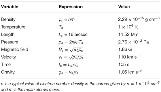
Table 1. Parameters used for non-dimensionalization.

In non-dimensionalized form, the full set of MHD equations are given as

$\begin{array}{r}\frac{\partial \rho }{\partial t}+\nabla ·(\rho \text{v})=-{\nu }_{\rho }(\rho -{\rho }_0),\\ \rho \frac{D\text{v}}{Dt}=-\nabla p+J\times B+\rho g+\nabla ·(\nu \rho \nabla \text{v}),\\ \frac{\partial B}{\partial t}=\nabla \times (v\times B),\\ \frac{\partial T}{\partial t}+\nabla ·(Tv)=(2-\gamma )T\nabla ·v.& (1)\end{array}$

where $J=\nabla \times B$, ν is the kinetic viscosity, and γ is the adiabatic index.

Note that we artificially add a source term −ν_ρ(ρ − ρ₀) to the continuity equation, where ρ₀ is the density at the initial time t = 0 (or some prescribed form), and ν_ρ is a prescribed coefficient. This term is used to avoid a ever-decreasing of the density in the strong magnetic field region, which we often encounter in the very low-β simulation. It can maintain the maximum Alfvén speed in a reasonable level, which may otherwise increase and make the iteration time step smaller and smaller and the long-term simulation unmanageable. Specifically, this source term is a Newton relaxation of the density to its initial value by a time scale of

$\begin{array}{ll}{\tau }_{\rho }=\frac{1}{{\nu }_{\rho }}=20{\tau }_{\text{A}},& (2)\end{array}$

where τ_A = 1/v_A is the Alfvén time with length of 1 (the length unit) and the Alfvén speed $v_{\text{A}}=B/\sqrt{\rho }$. Thus, it is sufficiently large to avoid its influence on the fast dynamics of Alfvénic time scales. As a result, we used ν_ρ = 0.05v_A in all the simulation in this paper.

No explicit resistivity is used in the magnetic induction equation, but magnetic reconnection is still allowed through numerical diffusion when a current layer is sufficiently narrow such that its width is close to the grid resolution. In the energy (or temperature) equation, we set γ = 1 for simplicity, such that the energy equation describes an isothermal process¹. The kinetic viscosity ν will be given with different values when needed, which is described in the following sections.

3. Construction of an Initial MHD Equilibrium

We first constructed an initial MHD equilibrium based on a single vector magnetogram taken for time of 00:00 UT on 2014 September 8 by SDO/HMI. Such an equilibrium is assumed to exist when the corona is not in the eruptive stage, and is crucial for starting our subsequent data-driven evolution. The vector magnetogram is preprocessed to reduce the Lorentz force and is further smoothed to filter out the small-scale structures that are not sufficiently resolved in our simulation. Reduction of the Lorentz force is helpful for reaching a more force-free equilibrium state [e.g., 27], and smoothing is also necessary to mimic the magnetic field at the coronal base rather directly the photosphere, because the lower boundary of our model is placed at the base of the corona [28]. The preprocessing is done using a code developed by Jiang et al. [29], which is originally designed for NLFFF extrapolation using the HMI data [30]. Specifically, the total Lorentz force and torque are quantified by two surface integrals associated with three components of the photospheric magnetic field, and an optimization method is employed to minimize these two functions by modifying the magnetic field components within margins of measurement errors. Then Gaussian smoothing with FWHM of 8 arcsec is applied to all the three components of the magnetic field. Figure 1 compares the original HMI vector magnetogram with the preprocessed one as well as the final smoothed version. Using the vertical component B_z of this preprocessed and smoothed magnetogram, a potential field is extrapolated and used as the initial condition of the magnetic field in the MHD model.

FIGURE 1

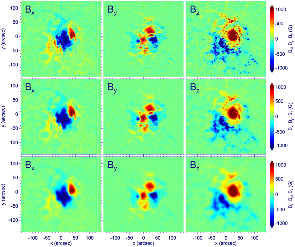
Figure 1. Comparison of the original HMI vector magnetogram for time of 00:00 UT on 2014 September 8 (Top), the preprocessed one (Middle), and the final smoothed one (Bottom). From left to right are shown for magnetic field components B_x, B_y, and B_z, respectively.

In addition to the magnetic field, an initial plasma as the background atmosphere is also needed to start the MHD simulation. We used an isothermal plasma in hydrostatic equilibrium. It is stratified by solar gravity with a density ρ = 1 at the bottom and a uniform temperature of T = 1. Using this typical coronal plasma, we did not directly input the magnetic field into the model but multiplies it with a factor of 0.05 such that the maximum of magnetic field strength in normalized value is approximately 50~100 in the model. If using the original values of magnetic field, its strength (and the characteristic Alfvén speed) near the lower surface is too larger, which will be a too heavy burden on computation as the time step of our simulation is limited by the CFL condition. With the reduced magnetic field, we further modified the value of solar gravity to avoid an unrealistic large plasma β (and small Alfvén speed) in the corona. This is because if using the real number of the solar gravity (g_⊙ = 274 m s${}^{-2}/g_s=0.26$), it results in a pressure scale height of H_p = 3.8, by which the plasma pressure and density decay with height much slower than the magnetic field. With the weak magnetic field strength we used, the plasma β will increase with height very fast to above 1, which is not realistic in the corona. To make the pressure (and density) decrease faster in the lower corona, we modified the gravity as

$\begin{array}{ll}g=\frac{1.5H_p{g}_{\odot }}{{(1+0.15z)}^2}.& (3)\end{array}$

By this, we got a plasma with β < 1 mainly within z < 10 and the smallest value is 5 × 10⁻³.

Then we input the transverse field of the smoothed magnetogram to the model. This is done by modifying the transverse field on the bottom boundary incrementally using linear extrapolation from the potential field to the vector magetogram in time with a duration of 1 t_s until it matches the vector magnetogram. This will drive the coronal magnetic field to evolve away from the initial potential state, since the change of the transverse field will inject electric currents and thus Lorentz forces, which drive motions in the computational volume. Note that in this phase all other variables on the bottom boundary are simply fixed, thus the velocity remaining zero. This is somewhat un-physical since the Lorentz force will introduce non-zero flows on the bottom boundary, but it provides a simple and “safe” way (avoiding numerical instability) to bring the transverse magnetic field into the model. Once the magnetic field on the bottom surface is identical to that of the vector magnetogram, the system is then left to relax to equilibrium with all the variables (including the magnetic field) on the bottom boundary fixed. To avoid a too large velocity in this phase such that the system can relax faster, we set the kinetic viscosity coefficient as ν = 0.5Δx²/Δt, where Δx is the local grid spacing and Δt the local time step, determined by the CFL condition with the fastest magnetosonic speed. Actually this is the largest viscosity one can use with given grid size Δx and time step Δt, because the CFL condition for a purely diffusive equation with diffusion coefficient ν requires Δt ≤ 0.5Δx²/ν.

For the purpose of minimizing the numerical boundary influences introduced by the side and top boundaries of the computational volume, we used a sufficiently large box of (−32, −32, 0) < (x, y, z) < (32, 32, 64) embedding the field of view of the magnetogram of (−8.75, −8.25) < (x, y) < (8.75, 8.25). The full computational volume is resolve by a non-uniform block-structured grid with adaptive mesh refinement (AMR), in which the highest and lowest resolution are Δx = Δy = Δz = 1/16 (corresponding to 1 arcsec or 720 km, matching the resolution of the vector magnetogram) and 1/2, respectively. The AMR is controlled to resolve with the smallest grids the regions of strong magnetic gradients and current density. The magnetic field outside of the area of the magnetograms on the lower boundary is given as zero for the vertical component and simply fixed as the potential field for the transverse components. On the side and top boundaries, we fixed the plasma density, temperature, and velocity. The horizontal components of magnetic field are linearly extrapolated from the inner points, while the normal component is modified according to the divergence-free condition to avoid any numerical magnetic divergence accumulated on the boundaries.

In Figure 2, the curves colored in black show the evolution of the magnetic and kinetic energies integrated for the computational volume, and the residual of the magnetic field of two consecutive time steps which is defined as

$\begin{array}{ll}{\text{Res}}_B=\sqrt{\frac{1}{3}{\displaystyle \sum _{\delta =x,y,z}}\frac{{\sum }_i{\left(B_{i\delta }^k-B_{i\delta }^{k-1}\right)}^2}{{\sum }_i{\left(B_{i\delta }^k\right)}^2}},& (4)\end{array}$

where the indices k and k − 1 refer to the two consecutive time steps and i goes through all the mesh points. It can be seen that the magnetic energy increases sharply in a few time units², reaching ~1.4 of the potential field energy E₀ (here $E_0=1.2\times 10^{33}$ erg when scaled to the realistic value in the corona), and then keeps almost constant during the relaxing phase with bottom boundary fixed. Very similar, the kinetic energy first increases and later keeps on the level of 3 × 10⁻³ of E₀. The residual of the magnetic field increases in the first t_s as we continually modified the transverse field at the bottom boundary which drives quickly the evolution of the field in the corona. Then it decreases to below 10⁻⁵ with a time duration of 20t_s, which indicates that the magnetic field reaches a quasi-equilibrium state.

FIGURE 2

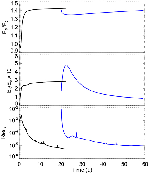
Figure 2. Evolutions of the total magnetic energy, kinetic energy, and residual of magnetic field in the process of the constructing the initial MHD equilibrium. The black curves show the results for the first evolution phase, and the blue ones show that for the second, “deeper” evolution phase.

To make the field even closer to equilibrium, we carried out a “deeper” relaxation by running the model again, which is started with the relaxed magnetic field obtained at t = 20t_s and the initially hydrostatic plasma. Now we reduce the kinetic viscosity to ν = 0.05Δx²/Δt, i.e., an order of magnitude smaller than the previously used one, which will let the magnetic field relax further. Furthermore, the magnetic field at the boundary boundary is allowed to evolve in a self-consistent way by assuming the bottom boundary as a perfectly line-tying and fixed (i.e., $v=0$) surface of magnetic field lines. However, such a line-tying condition does not indicate that all magnetic field components on the boundary are fixed, because even though the velocity $v$ is given as zero on the bottom boundary, it is not necessarily zero in the neighboring inner points. To self-consistently update the magnetic field, we solve the magnetic induction equation on the bottom boundary. Slightly different from the one in the main Equations (1), the induction equation at the bottom surface is given as

$\begin{array}{ll}\frac{\partial B}{\partial t}=\nabla \times (v\times B)+{\eta }_{\text{stable}}\nabla {\perp }^{2}B,& (5)\end{array}$

where we added a surface diffusion term defined by using a surface Laplace operator as $\nabla {\perp }^2=\frac{{\partial }^2}{\partial x^2}+\frac{{\partial }^2}{\partial y^2}$ with a small resistivity for numerical stability near the PIL ${\eta }_{\text{stable}}=1\times 10^{-3}{e}^{-B_z^2}$, since the magnetic field often has the strongest gradient on the photosphere around the main PIL. The surface induction Equation (5) in the code is realized by second-order difference in space and first-order forward difference in time. Specifically, on the bottom boundary (we do not use ghost cell), we first compute $v\times B$, and then use central difference in horizontal direction and one-sided difference (also 2nd order) in the vertical direction to compute the convection term ∇ × (v × B). The surface Laplace operator is also realized by central difference.

The curves colored in blue in Figure 2 show the evolution of different parameters during this relaxation phase³. Initially one can see a fast decrease of the magnetic energy because the magnetic field becomes more relaxed. As the viscosity is reduced significantly, the kinetic energy first increases, as driven by the residual Lorentz force of the magnetic field, to almost $5\times 10^{-3}{E}_0$. Then as the magnetic field relaxed, the kinetic energy decreases fast to eventually less than $10^{-3}{E}_0$, which is a very low level. The residual of magnetic field of two consecutive time steps also decreases to 10⁻⁵. These values show that the magnetic field reaches an excellent equilibrium.

Figure 3 shows the 3D magnetic field lines of the final relaxed MHD equilibrium. Note that the field lines are false-colored by the values of the force-free factor defined as $\alpha =J·B/B^2$, which indicates how much the field lines are non-potential. For a force-free field, this parameter is constant along any given field line. As can be seen, the magnetic field is close to a perfect force-free one since the color is nearly the same along any single field line. In the core of the configuration, the field lines are sheared significantly along the PIL, and thus have large values of α and current density. On the other hand, the overlying field is almost current-free or quasi-potential field with α~0, which plays the role of strapping field that confines the inner sheared core. Such a configuration is typical for eruption-productive ARs [e.g., 5, 31–34].

FIGURE 3

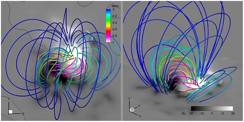
Figure 3. 3D magnetic field of the MHD equilibrium based on the magnetogram taken for 00:00 UT on 2014 September 8. The thick lines are magnetic field lines and are pseudo-colored by value of the force-free parameter α. The background is shown with the magnetic flux distribution (i.e., B_z) on the bottom surface of the model.

4. Derive the Surface Flow Field

Based on the time sequence of vector magnetograms, it is straightforward to derive the surface velocity by employing the DARE4VM code developed by [19]. The differential affine velocity estimator (DAVE) was first developed for estimating velocities from line-of-sight magnetograms, and was then modified to directly incorporate horizontal magnetic fields to produce a differential affine velocity estimator for vector magnetograms (DAVE4VM). We use the SHARP data with cadence of 12 min and pixel size of 1 arcsec (by rebinning the original data with pixel size of 0.5 arcsec), and first of all, we fill the data gap using a linear interpolation in the time domain to generate a complete time series of 3 days from 00:00 UT on 2014 September 8 to 24:00 UT on September 10 with cadence of 12 min. Then we input the time series of vector magnetogram (rebinned as 1 arcsec per pixel) in the DAVE4VM code. A key parameter needed by the DAVE4VM code is the window size, and here we use 19 pixels, following [35] and [36]. After obtaining the surface velocity, we first reset those in the weak-field region (with total magnetic field strength below 100 G) as zero, because there are large errors and unresolved scales in these regions. Figure 4 shows evolution of the Poynting flux dE/dt, which is defined by

$\begin{array}{ll}\frac{\text{d}E}{\text{d}t}=\frac{1}{{\mu }_0}{\displaystyle \underset{S}{\int }}\left[(B_x^2+B_y^2)v_z-(B_x{v}_x+B_y{v}_y)B_z\right]\text{d}x\text{d}y,& (6)\end{array}$

where S is the photospheric surface, and its time accumulation E_acc, as computed by using the surface flow (v_x, v_y, v_z) and the magnetic field. It can be seen that, except the data gap intervals⁴, the magnetic energy is continually injected in the corona through the photosphere, and in the 3 days, it gains ~5 × 10³² erg.

FIGURE 4

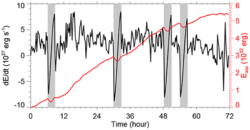
Figure 4. Evolution of Poynting flux (black line) and the accumulated energy (red line) which is time integration of the Poynting flux. The gray bars denote the data gaps of the vector magnetograms for which a simple linear interpolation in time is used to fill.

Before being input into the model, the flow data are also needed to be smoothed. We smoothed the time series of flow maps in both the time and space domains, with a Gaussian FWHM of 6 h (i.e., 30 time snapshots) and 8 arcsec, respectively, which is finally input to the data-driven model. Figure 5 shows 4 snapshots of the surface velocity after smoothing. The speed of the flow is generally a few hundreds of meters per second and the main feature is a clear and persistent rotation of the main sunspot. Note that during the 3 days the basic configuration of the photospheric magnetic flux distribution is rather similar with only somewhat dispersion. So the magnetic energy injection should come mainly from the transverse rotational flows. In addition to the rotational flow, we can see very evident diverging flow existing persistently near the boundary of the sunspot.

FIGURE 5

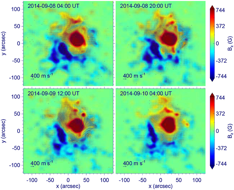
Figure 5. Four snapshots of the surface flows (the final smoothed version) as derived using the DAVE4VM code.

5. Data-Driven Simulation

We input the surface velocity at the bottom boundary to drive the evolution of the model, by starting the simulation from the solution obtained from the time point of t = 58 in the relaxation phase (see Figure 2) as described in section 3. Here to save computing time, the cadence of the input flow maps, which is originally 12 min, was increased by 68.6 times when inputting into the MHD model. As a result, an unit of time in the simulation, t_s, corresponds to actually t_s × 68.6 = 7200 s, i.e., 2 h, in the HMI data. Compressing of the time in HMI data is justified by the fact that the speed of photospheric flows is often a few 100 m s⁻¹. So in our model settings, the evolution speed of the boundary field, even enhanced by a factor of 68.6, is still smaller by two orders of magnitude than the coronal Alfvén speed (on the order of 10³ km s⁻¹), and the quick reaction of the coronal field to the slow bottom changes should not be affected. The implementation of the bottom boundary conditions is the same as that for the deeper relaxation phase described in section 3. That is, on the bottom surface, we solved the Equation (5) to update all the three components of magnetic field with the flow field prescribed by those derived in section 4, while the plasma density and temperature are simply fixed. In the driven-evolution phase, the kinetic viscosity is also used as the smaller one ν = 0.05Δx²/Δt, which corresponds to a Reynolds number of 10 for the length of a grid cell Δx.

We show an approximately 2-day (a duration of 26t_s or 52 h in reality) evolution of the MHD system as an example, while the further evolution associated with an eruption and the physical mechanisms will be left for future study. Figure 6 presents the global energy evolutions. It can be seen the magnetic energy (the black line in the top panel) increases monotonously as driven by the surface flows. By the end of our simulation, it reaches approximately 1.8 times of the initial potential energy, and thus the total magnetic energy obtained in this driving phase is $(1.8-1.4)\times E_0\approx 4.8\times 10^{32}$ erg. On the other hand, the kinetic energy (bottom panel of Figure 6) keeps below the level of $1\times 10^{-3}{E}_0$ with a mild increase, which indicates that the system remains a stable, quasi-static evolution. In the top panel of Figure 6 we also plots the time integration of total Poynting flux (the blue line), using the magnetic field and the flow field on the bottom boundary of the simulation, which is the energy injected into the volume from the bottom boundary through the surface flow. If our boundary condition is accurately implemented, the energy injected from the bottom surface should match the magnetic energy obtained in the computational volume, since other energies are negligible if compared with the magnetic energy. As can be seen, the trend of magnetic energy evolution (the black line) matches rather well that of the energy input by the surface flow (the blue line), albeit a small numerical error that increases slowly the total magnetic energy, which is also seen in the relaxation phase as shown in Figure 2. It is worthy noting that the magnetic energy evolution is also in good agreement with the accumulated magnetic energy as derived from directly the observation data (the red line, which is the same value shown in Figure 4 but multiplied by a factor of 0.05² because the field input to the model is multiplied by 0.05) as calculated in section 4, which suggests that our data-driven model can reliably reproduce the magnetic energy injection into the corona through the photospheric motions. The small difference between the observation-derived and simulated energies might be due to the smoothing of the velocity since it filters out the small-scale flows that also contribute to the total Poynting flux.

FIGURE 6

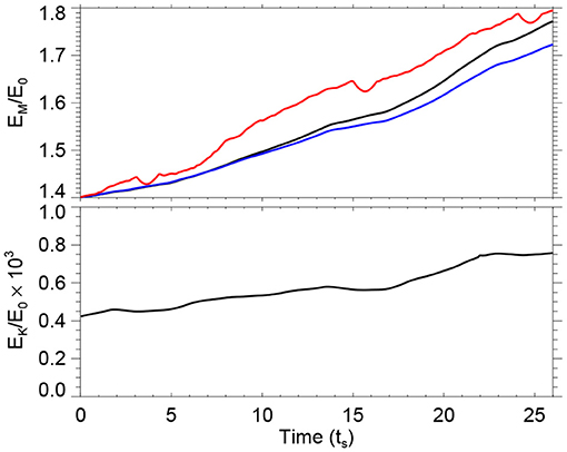
Figure 6. Magnetic energy (Top) and kinetic energy (Bottom) evolution of the MHD system as driven by the photospheric flows. The black lines represent the values of the volume-integrated energies. The blue line in the top panel shows the time integration of the total Poynting flux on the bottom surface from the simulation. The red line shows the accumulated magnetic energy from directly the observation data, i.e., the same one shown in Figure 4.

Figure 7 (and its attached animation) shows the 3D magnetic field lines and their evolution in comparison with SDO/AIA image of coronal loops in the 94 Å wavelength which highlights the hot, core coronal loops in the AR. Overall, we can see a slow stressing of the field lines mainly through the sunspot rotational flow. It renders the core field lines to form a more and more coherent S shape, which resembles the observed sigmoid structure in the core of the AR. The increase of non-potentiality can also be seen from the increase of the force-free factor α in the core region. Figure 8 shows evolution of the surface magnetic flux distribution (see also the animation attached to Figure 7). The four snapshots are taken for the same times given in Figure 5, and thus comparing Figure 8 with Figure 5 shows the difference between the simulated magnetograms and the observed ones. In addition to the rotation of the main sunspot, an evident feature is the enhancement of the field strength along the PIL. This is owing to the divergence flow from the edge of the sunspot, which continually convect the magnetic flux to the PIL. Such pileup of magnetic flux near the PIL, however, is not seen in the observed magnetograms (Figure 5), which rather show field decaying. Such decaying of magnetic flux is likely due to the global turbulent diffusion of photospheric magnetic field by granular and supergranular convection [37] and other small-scale turbulence and flux cancellations in the photosphere, which is not being recovered by the DAVE4VM code and thus not reproduced in our simulation.

FIGURE 7

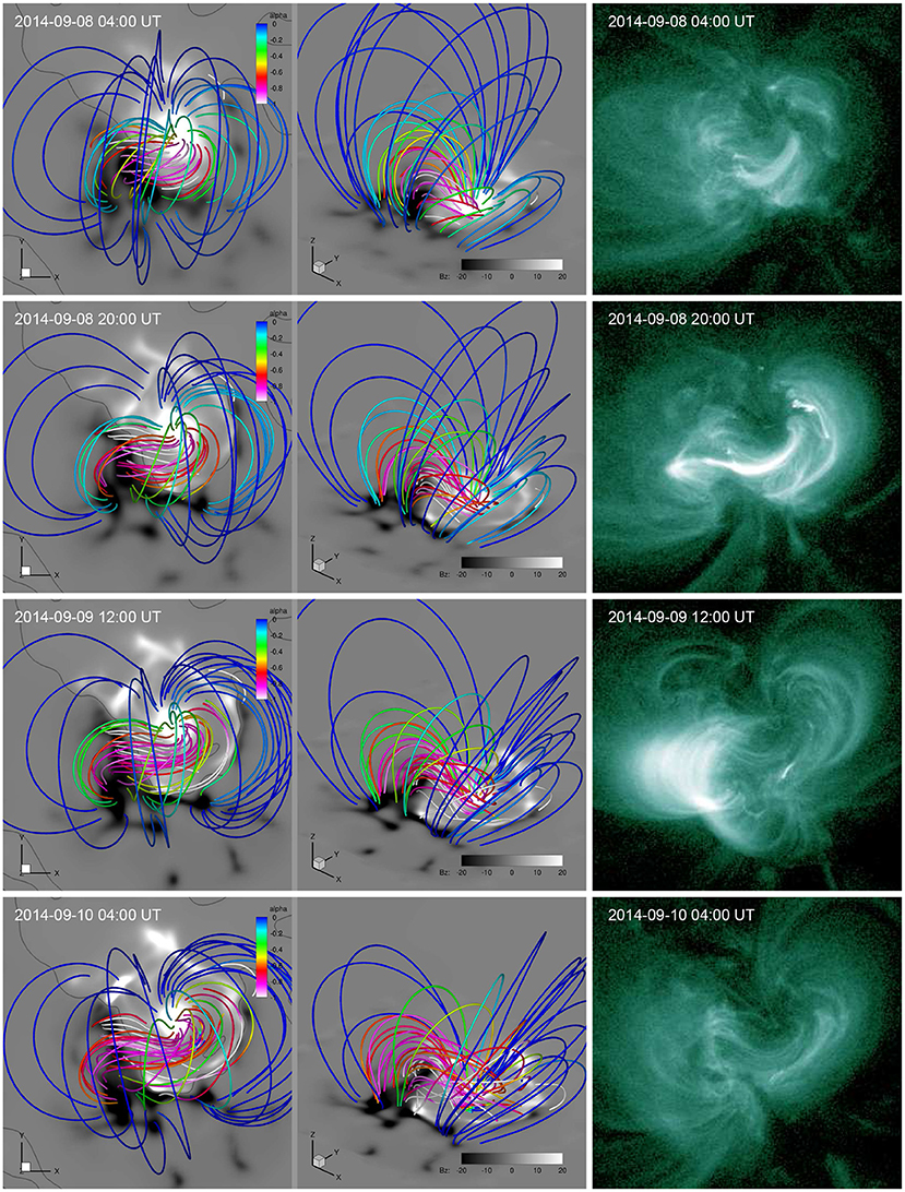
Figure 7. Evolution of the magnetic field lines (shown in different view angles in the left and middle columns) and their comparison with observed coronal loops observed in EUV wavelength of 94 Å by SDO/AIA (right column). The field lines are shown in the same format in Figure 3. An animation of the magnetic field evolution is attached for this figure.

FIGURE 8

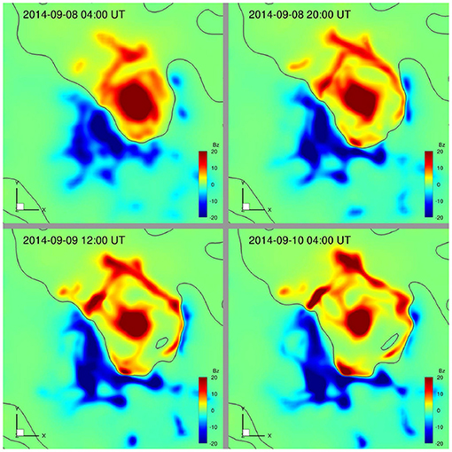
Figure 8. Evolution of magnetic flux distribution on the bottom surface in the simulation, shown for 4 snapshots of the same times shown in Figure 5.

6. Conclusions

This paper is devoted to the description of a new approach of data-driven modeling of solar AR magnetic field evolution, in which, we have for the first time utilized directly the photospheric velocity field from DAVE4VM to drive a full-MHD model. To setup the initial conditions, we used a special MHD relaxation approach with sufficiently small kinetic viscosity to construct a true MHD equilibrium based on a single vector magnetogram. Then we derived the photospheric surface flows from a time series of observed magentograms based on the DAVE4VM method. The surface flows were finally inputted, again in time sequence, to the bottom boundary of the MHD model to self-consistently update the magnetic field at every time step, which is implemented by solving directly the magnetic induction equation at the bottom boundary using finite difference method.

We applied this data-driven model to study the magnetic field evolution of AR 12158 with SDO/HMI vector magnetograms. The initial MHD equilibrium is calculated using magnetogram observed for 00:00 UT on 2014 September 8, and a 2-day duration of the AR evolution is then simulated using the data-driven MHD model. Overall, the evolution is characterized by a slow stress of the field lines mainly through the rotational flow of the AR's leading sunspot, which makes the core field lines to forms an coherent S shape consistent with the sigmoid structure as seen in the AIA images. Such evolution proceeds in a quasi-static way since the kinetic energy of the system remains less than its magnetic energy by three orders of magnitude, while the magnetic energy increases monotonously as driven by the surface flow, and reaches approximately double of the initial potential energy by the end of the simulation. The magnetic energy obtained in the simulation during the surface driving phase matches closely the accumulated magnetic energy as calculated directly from the original vector magnetogram with the DAVE4VM derived flow field.

With the surface flow specified at the bottom boundary, the magnetic field can be updated self-consistently by solving the induction equation at the surface boundary. However, our simulation shows that discrepancy arises between the simulated magnetic field at the bottom surface with the original magnetograms. That is, in the simulation, magnetic flux are significantly enhanced along the PIL, owing to the divergence flow from the edge of the sunspot, whereas in the observed magnetograms such pileup of magnetic flux near the PIL is not seen, which rather shows field decaying. In the next step, we will try to use some ad-hoc flux cancellation near the PIL, for which a straightforward way is to increase the value of η_stable in Equation (5), such that the flux diffusion speed is comparable to that of the flux pileup. In the future, we will consider to include the global diffusion of photospheric magnetic field by granular and supergranular convection to simulate more realistically the magnetic field evolution. On the other hand, the discrepancy might result from errors in the vector magnetograms, since these errors can introduce spurious flows with the DAVE4VM code and thus influences our simulation. To elucidate this, we will test our model with error-free magnetograms from recent convective flux-emergence simulations [e.g., 38–40] as the ground-truth data.

Our ultimate purpose is to use the model to study how the coronal field, as driven by the slow photospheric motions, reaches a unstable state and runs into eruption. From this, we will be able to investigate in details the topology of the evolving magnetic field leading to the eruption, to see whether it forms a magnetic flux rope and becomes ideally unstable [e.g., 41, 42], or, a simply sheared arcade with a interally-formed current sheet to trigger flare reconnection [43], which would be helpful for resolving the long-standing debates on the triggering mechanism of solar eruptions [44].

Data Availability Statement

The original contributions presented in the study are included in the article/supplementary material, further inquiries can be directed to the corresponding author/s.

Author Contributions

CJ developed the numerical model, performed the result analysis, and wrote the draft. All authors participated in discussions and revisions on the manuscript.

Conflict of Interest

The authors declare that the research was conducted in the absence of any commercial or financial relationships that could be construed as a potential conflict of interest.

The reviewer YG declared a past co-authorship with one of the authors CJ to the handling editor.

Acknowledgments

This work is jointly supported by National Natural Science Foundation of China (NSFC 41822404, 41731067, 41574170, and 41531073), the Fundamental Research Funds for the Central Universities (Grant No. HIT.BRETIV.201901), and Shenzhen Technology Project JCYJ20190806142609035. Data from observations are courtesy of NASA SDO. The computational work was carried out on TianHe-1(A), National Supercomputer Center in Tianjin, China. We are grateful to the reviewers for helping to improve the paper.

Footnotes

1. ^Although in this case we can simply discard the energy equation by setting the temperature as a constant, we still keep the full set of equations in our code which can thus describe either the isothermal or adiabatic process by choose different value of γ.

2. ^Note that at the very beginning the magnetic energy actually decreases shortly for about 0.5t_s, which is unphysical as the potential field energy is in principle the lowest energy with a given magnetic flux distribution on the bottom boundary. Such an unphysical evolution is a result of the fact that we modified directly the transverse magnetic field on the bottom boundary in an unphsyical way.

3. ^Note that the initial values of the blue curves (the deeper relaxation phase) do not equal to the values of the black curves at t = 20t_s although the deeper relaxation phase starts from that time point. This is because in the deeper relaxation process, there are three ways different from the initial relaxation one: (1) the velocity is reset to zero and the plasma is reset to hydrostatic state, thus the kinetic energy is reset to zero; (2) the viscosity is abruptly reduced by an order of magnitude; (3) the boundary condition is changed. Furthermore, not data of every time step in the run is recorded, thus small difference is shown in the magnetic energy of the initial value of the blue line (which is not exactly for the time of t = 20t_s) from the t = 20t_s of the black line.

4. ^During the data gaps the Poynting flux is found to become negative adruptly, which might be a result of our simple linear interpolation in filling the gaps of the magnetograms. More optimized method for filling the data gaps will be considered to recover a more consistent evolution of Poynting flux.

References

1. Wiegelmann T, Sakurai T. Solar force-free magnetic fields. Liv Rev Solar Phys. (2012) 9:5. doi: 10.12942/lrsp-2012-5

CrossRef Full Text | Google Scholar

2. Wu ST, Wang AH, Liu Y, Hoeksema JT. Data-driven magnetohydrodynamic model for active region evolution. Astrophys J. (2006) 652:800–11. doi: 10.1086/507864

CrossRef Full Text | Google Scholar

3. Feng X, Jiang C, Xiang C, Zhao X, Wu ST. A data-driven model for the global coronal evolution. Astrophys J. (2012) 758:62. doi: 10.1088/0004-637X/758/1/62

CrossRef Full Text | Google Scholar

4. Cheung MCM, DeRosa ML. A method for data-driven simulations of evolving solar active regions. Astrophys J. (2012) 757:147. doi: 10.1088/0004-637X/757/2/147

CrossRef Full Text | Google Scholar

5. Jiang CW, Wu ST, Feng XS, Hu Q. Data-driven MHD simulation of a flux-emerging active region leading to solar eruption. Nat Commun. (2016) 7:11522. doi: 10.1038/ncomms11522

CrossRef Full Text | Google Scholar

6. Leake JE, Linton MG, Schuck PW. Testing the accuracy of data driven MHD simulations of active region evolution. Astrophys J. (2017) 838:113. doi: 10.3847/1538-4357/aa6578

CrossRef Full Text | Google Scholar

7. Inoue S, Kusano K, Büchner J, Skála J. Formation and dynamics of a solar eruptive flux tube. Nat Commun. (2018) 9:174. doi: 10.1038/s41467-017-02616-8

PubMed Abstract | CrossRef Full Text | Google Scholar

8. Hayashi K, Feng X, Xiong M, Jiang C. Magnetohydrodynamic simulations for solar active regions using time-series data of surface plasma flow and electric field inferred from helioseismic magnetic imager vector magnetic field measurements. Astrophys J. (2019) 871:L28. doi: 10.3847/2041-8213/aaffcf

CrossRef Full Text | Google Scholar

9. Guo Y, Xia C, Keppens R, Ding MD, Chen PF. Solar magnetic flux rope eruption simulated by a data-driven magnetohydrodynamic model. Astrophys J. (2019) 870:L21. doi: 10.3847/2041-8213/aafabf

CrossRef Full Text | Google Scholar

10. Pomoell J, Lumme E, Kilpua E. Time-dependent data-driven modeling of active region evolution using energy-optimized photospheric electric fields. Sol Phys. (2019) 294:41. doi: 10.1007/s11207-019-1430-x

PubMed Abstract | CrossRef Full Text | Google Scholar

11. Toriumi S, Takasao S, Cheung MCM, Jiang C, Guo Y, Hayashi K, et al. Comparative study of data-driven solar coronal field models using a flux emergence simulation as a ground-truth data set. Astrophys J. (2020) 890:103. doi: 10.3847/1538-4357/ab6b1f

CrossRef Full Text | Google Scholar

12. Yang WH, Sturrock PA, Antiochos SK. Force-free magnetic fields – The magneto-frictional method. Astrophys J. (1986) 309:383. doi: 10.1086/164610

CrossRef Full Text | Google Scholar

13. Inoue S. Magnetohydrodynamics modeling of coronal magnetic field and solar eruptions based on the photospheric magnetic field. Prog Earth Planet Sci. (2016) 3:19. doi: 10.1186/s40645-016-0084-7

CrossRef Full Text | Google Scholar

14. Nakagawa Y. Evolution of solar magnetic fields - a new approach to mhd initial-boundary value problems by the method of near-characteristics. Astrophys J. (1980) 240:275. doi: 10.1086/158232

CrossRef Full Text | Google Scholar

15. Nakagawa Y, Hu YQ, Wu ST. The method of projected characteristics for the evolution of magnetic arches. Astron Astrophys. (1987) 179:354–70.

Google Scholar

16. Wu ST, Wang JF. Numerical tests of a modified full implicit continuous eulerian (FICE) Scheme with projected normal characteristic boundary conditions for MHD flows. Comput Methods Appl Mech Eng. (1987) 64:267–82. doi: 10.1016/0045-7825(87)90043-0

CrossRef Full Text | Google Scholar

17. Hayashi K. magnetohydrodynamic simulations of the solar corona and solar wind using a boundary treatment to limit solar wind mass flux. Astrophys J Suppl. (2005) 161:480–94. doi: 10.1086/491791

CrossRef Full Text | Google Scholar

18. Jiang C, Wu ST, Yurchyshyn VB, Wang H, Feng X, Hu Q. How did a major confined flare occur in super solar active region 12192. Astrophys J. (2016) 828:62. doi: 10.3847/0004-637X/828/1/62

CrossRef Full Text | Google Scholar

19. Schuck PW. Tracking vector magnetograms with the magnetic induction equation. Astrophys J. (2008) 683:1134. doi: 10.1086/589434

CrossRef Full Text | Google Scholar

20. Priest ER, Forbes TG. The magnetic nature of solar flares. Astron Astrophys Rev. (2002) 10:313–17. doi: 10.1007/s001590100013

CrossRef Full Text | Google Scholar

21. Vemareddy P, Cheng X, Ravindra B. Sunspot rotation as a driver of major solar eruptions in the NOAA active region 12158. Astrophys J. (2016) 829:24. doi: 10.3847/0004-637X/829/1/24

CrossRef Full Text | Google Scholar

22. Zhao J, Gilchrist SA, Aulanier G, Schmieder B, Pariat E, Li H. Hooked flare ribbons and flux-rope related QSL footprints. Astrophys J. (2016) 823:62. doi: 10.3847/0004-637X/823/1/62

CrossRef Full Text | Google Scholar

23. Zhou GP, Zhang J, Wang JX. Observations of magnetic flux-rope oscillation during the precursor phase of a solar eruption. Astrophys J. (2016) 823:L19. doi: 10.3847/2041-8205/823/1/L19

CrossRef Full Text | Google Scholar

24. Duan A, Jiang C, Hu Q, Zhang H, Gary GA, Wu ST, et al. Comparison of two coronal magnetic field models to reconstruct a sigmoidal solar active region with coronal loops. Astrophys J. (2017) 842:119. doi: 10.3847/1538-4357/aa76e1

CrossRef Full Text | Google Scholar

25. Lee H, Magara T. MHD Simulation for investigating the dynamic state transition responsible for a solar eruption in active region 12158. Astrophys J. (2018) 859:132. doi: 10.3847/1538-4357/aabfe6

CrossRef Full Text | Google Scholar

26. Jiang CW, Feng XS, Zhang J, Zhong DK. AMR Simulations of magnetohydrodynamic problems by the CESE method in curvilinear coordinates. Sol. Phys. (2010) 267:463–491. doi: 10.1007/s11207-010-9649-6

CrossRef Full Text | Google Scholar

27. Wiegelmann T. Optimization code with weighting function for the reconstruction of coronal magnetic fields. Sol Phys. (2004) 219:87–108. doi: 10.1023/B:SOLA.0000021799.39465.36

CrossRef Full Text | Google Scholar

28. Jiang C, Toriumi S. Testing a data-driven active region evolution model with boundary data at different heights from a solar magnetic flux emergence simulation. Astrophys J. (2020) 903:11. doi: 10.3847/1538-4357/abb5ac

CrossRef Full Text | Google Scholar

29. Jiang C, Feng X. Preprocessing the photospheric vector magnetograms for an nlfff extrapolation using a potential-field model and an optimization method. Sol Phys. (2014) 289:63–77. doi: 10.1007/s11207-013-0346-0

CrossRef Full Text | Google Scholar

30. Jiang C, Feng X. Extrapolation of the solar coronal magnetic field from SDO/HMI magnetogram by a CESE-MHD-NLFFF code. Astrophys J. (2013) 769:144. doi: 10.1088/0004-637X/769/2/144

CrossRef Full Text | Google Scholar

31. Schrijver CJ, DeRosa ML, Metcalf T, Barnes G, Lites B, Tarbell T, et al. Nonlinear force-free field modeling of a solar active region around the time of a major flare and coronal mass ejection. Astrophys J. (2008) 675:1637–44. doi: 10.1086/527413

CrossRef Full Text | Google Scholar

32. Sun X, Hoeksema JT, Liu Y, Wiegelmann T, Hayashi K, Chen Q, et al. Evolution of magnetic field and energy in a major eruptive active region based on SDO/HMI observation. Astrophys J. (2012) 748:77. doi: 10.1088/0004-637X/748/2/77

CrossRef Full Text | Google Scholar

33. Toriumi S, Wang H. Flare-productive active regions. Liv Rev Solar Phys. (2019) 16:3. doi: 10.1007/s41116-019-0019-7

CrossRef Full Text | Google Scholar

34. Duan A, Jiang C, He W, Feng X, Zou P, Cui J. A study of pre-flare solar coronal magnetic fields: magnetic flux ropes. Astrophys J. (2019) 884:73. doi: 10.3847/1538-4357/ab3e33

CrossRef Full Text | Google Scholar

35. Liu Y, Zhao J, Schuck PW. Horizontal flows in the photosphere and subphotosphere of two active regions. Sol Phys. (2013) 287:279–91. doi: 10.1007/s11207-012-0089-3

CrossRef Full Text | Google Scholar

36. Liu C, Deng N, Lee J, Wiegelmann T, Jiang C, Dennis B, et al. Three-dimensional magnetic restructuring in two homologous solar flares in the seismically active NOAA AR 11283. Astrophys J. (2014) 795:128. doi: 10.1088/0004-637X/795/2/128

CrossRef Full Text | Google Scholar

37. Wang Y, Nash AG, Sheeley NR Jr. Magnetic flux transport on the sun. Science. (1989) 245:712–718. doi: 10.1126/science.245.4919.712

PubMed Abstract | CrossRef Full Text | Google Scholar

38. Chen F, Rempel M, Fan Y. Emergence of magnetic flux generated in a solar convective dynamo. I. the formation of sunspots and active regions, and the origin of their asymmetries. Astrophys J. (2017) 846:149. doi: 10.3847/1538-4357/aa85a0

CrossRef Full Text | Google Scholar

39. Cheung MCM, Rempel M, Chintzoglou G, Chen F, Testa P, Martnez-Sykora J, et al. A comprehensive three-dimensional radiative magnetohydrodynamic simulation of a solar flare. Nat Astron. (2019) 3:160–6. doi: 10.1038/s41550-018-0629-3

CrossRef Full Text | Google Scholar

40. Toriumi S, Hotta H. Spontaneous generation of -sunspots in convective magnetohydrodynamic simulation of magnetic flux emergence. Astrophys J. (2019) 886:L21. doi: 10.3847/2041-8213/ab55e7

CrossRef Full Text | Google Scholar

41. Kliem B, Tr¨k¨ T. Torus instability. Phys Rev Lett. (2006) 96:255002. doi: 10.1103/PhysRevLett.96.255002

CrossRef Full Text | Google Scholar

42. Aulanier G, Tr¨k¨ T, Démoulin P, DeLuca EE. Formation of torus-unstable flux ropes and electric currents in erupting sigmoids. Astrophys J. (2010) 708:314–33. doi: 10.1088/0004-637X/708/1/314

CrossRef Full Text | Google Scholar

43. Moore RL, Sterling AC, Hudson HS, Lemen JR. Onset of the magnetic explosion in solar flares and coronal mass ejections. Astrophys J. (2001) 552:833–48. doi: 10.1086/320559

CrossRef Full Text | Google Scholar

44. Chen PF. Coronal mass ejections: models and their observational basis. Liv Rev Solar Phys. (2011) 8:1. doi: 10.12942/lrsp-2011-1

CrossRef Full Text | Google Scholar