Concurrent Empirical Magnetic Reconstruction of Storm and Substorm Spatial Scales Using Data Mining and Virtual Spacecraft

1. Introduction

Storms and substorms represent two major modes of magnetospheric activity and the resulting space weather (e.g., [1, 2]), which is reflected in the corresponding low- and high-latitude geomagnetic indices, e.g., Sym-H [3] and AL [4]. Substorms frequently occur during the development of storm main phases and to a lesser extent during the recovery phase [5]. Although the original idea of substorms viewed them as building blocks of storms [6], which is reflected in the names of these phenomena, that view is now strongly modified [7, 8], as it is clear that storms and substorms are related because of their common driver, the solar wind [9, 10]. Despite this, storm-time in-situ observations during substorm expansions show charged particles injected deep into the inner magnetosphere [11, 12]. Furthermore, statistical analyses of particle measurements from the RBPSICE and HOPE instruments on the Van Allen Probes identified an energization of the ring current during substorm expansions [13, 14]. Additionally, empirical magnetic field models found that the substorm expansion phase was correlated with an increase in the amount of current contained within the symmetric ring current (SRC) during both storm and non-storm substorms [15]. As both types of disturbances have dramatic impacts on the global configuration of the geomagnetic field and associated current systems, a concurrent description of storms and substorms and their phases is needed.

Since the development of the earliest empirical magnetic field models [16], the storm state of the magnetosphere was considered in their construction by binning the magnetometer data by storm activity level. Over time, empirical models became more complex in their description of the storm state, by incorporating additional current systems and making them functionally dependent on storm activity indices and solar wind conditions [17–20]. Data mining (DM) ushered in an entirely different approach to the empirical modeling of storms, the first of which was termed the TS07D model [21, 22]. The DM technique refits the model for each snapshot in time to a small subset of the entire magnetometer database. This subset of data is identified by mining the whole database for other time intervals when the magnetosphere was presumably in a similar storm state configuration, characterized using the storm index Sym-H, its derivative, and the solar wind electric field parameter $v{B}_z^{IMF}$. The DM algorithm employed in TS07D is the k-Nearest Neighbor (kNN) method [23], which is described in section 2.2. The first applications of the TS07D model were to investigate the global magnetic field and current system configuration of storms driven by different solar wind phenomena [22, 24].

In contrast to the storm state, until recently, inclusion of the description of the substorm state of the magnetosphere within empirical magnetic field models has been limited. Event-oriented approaches sought to describe the substorm growth phase by incorporating a magnetotail thin current sheet (TCS) into storm models and then adjusting the TCS to match particular event observations [25, 26]. Wire-models attempted to describe the substorm expansion by hand tailoring the substorm current wedge (SCW) [27–29]. Showcasing the flexibility of the DM approach, TS07D was customized to picture geomagnetic substorms [15, 30] by including the substorm index AL and its time derivative as binning parameters and by incorporating a TCS into the model structure. Termed the SST19 model, it was successful in reconstructing the primary substorm features of the magnetosphere including the stretching of the magnetotail associated with the enhancement of the TCS in the near-tail during the growth phase and the rapid dipolarization of the magnetotail along with the formation of the substorm current wedge during the expansion phase. It also revealed a connection between the substorm expansion phase and the ring current enhancement, seen as ≈ 1 MA increase in the dayside ring current during a non-storm substorm.

However, the resolution of the SST19 model was insufficient to fully resolve the innermost magnetosphere, in particular, it was unable to reconstruct the eastward component of the ring current. Earthward (r ≲ 4R_E) of the dominant westward ring current, the azimuthal component of the ring current changes sign becoming eastwardly oriented [31]. Assuming force-balance and pressure isotropy, the boundary between the eastward and westward oriented ring current identifies the location of the plasma pressure peak [32].

An advantage of the DM approach, which reflects a postulate of machine learning techniques, is that the addition of more high quality data sets allows for increasing model complexity. Thus, an obvious remedy to enable the model to more fully resolve the inner magnetosphere is to increase the resolution of the equatorial field, taking advantage of the numerous spacecraft missions that fly through this region (e.g., Van Allen Probes, THEMIS, Polar, Cluster). Indeed, several applications of the TS07D family of models have demonstrated this [33–36], but unlike SST19, the focus of these studies was largely limited to the inner magnetosphere. As this study reveals, the higher equatorial resolution used for those inner magnetosphere investigations overfits the near-tail, introducing numerous artifacts in the reconstruction of the magnetic fields and electric currents. On one hand, this is a key advantage of the TS07D approach, that is, the resolution of the model can be customized to the particular region of interest, but on the other hand, it is also a shortcoming in that no single resolution is adequate for the entirety of the spatial domain of the magnetosphere. This dilemma is discussed in detail in section 2.4.

In section 3 we present a simple yet effective solution for how to concurrently reconstruct both the inner magnetosphere necessary for storm features and the near-tail needed for the description of substorms. Two separate models are constructed with varying equatorial resolutions, one customized for the inner and the other for the near-tail regions. Both models are then sampled in their respective regions to synthesize a distribution of virtual magnetic field observations dense enough to fit a third model, effectively merging the two other models while maintaining the divergenceless property of the magnetic and current density fields. The focus of this study will be a pair of non-storm time substorms that occurred on 8 March 2009. These were previously analyzed by Stephens et al. [15] and as such represent a good test case for comparing the merged model to the SS19 model, as is described in section 3.2.

2. Using Data Mining to Empirically Picture the Magnetosphere

2.1. Magnetic Field Architecture

Empirical magnetic field models are designed with two primary considerations: the spatial structure of the current systems and their dynamical evolution over time. For describing the spatial structure, it is useful to model each current system individually as a sub-model termed a module [20]. The total magnetic field B_tot is then the sum of magnetic field of each module along with the internal field, e.g., B_tot = B_FAC + B_PRC + B_SRC + B_tail + B_MP + B_int corresponding to the magnetic field from the field-aligned currents (FACs), partial and symmetric ring current (PRC and SRC), the cross-tail current, and the magnetopause (or Chapman-Ferraro) currents, respectively. The internal field, B_int, is readily determined with ground magnetometers and as such is not in the scope of this research and the IGRF model [37] is used to represent it. Earlier models sought to define these modules by hand, crafting a mathematical description based on the theoretical picture of the current system (e.g., [19]). Each of these modules will have non-linear parameters that determine their spatial scales and linear amplitude coefficients controlling their intensity. For example, a magnetic field module could take the form ${\text{B}}^{\prime }(\text{r})=a_1\text{B}(\text{r};{\beta }_1)$, where a₁ is the amplitude coefficient and β₁ is a non-linear parameter defining the module's mathematical structure (e.g., the current system's spatial scale size or thickness). The total model's set of a_is and β_js are then fit to the available magnetometer data [20]. The dynamical evolution of the current systems can thus be introduced by simply making a_is and β_js functions of time. Some of the earliest models achieved this straightforwardly by binning the magnetometer data by the K_p storm index and performing separate fits for each bin [16, 38]. The proceeding models instead opted to make a_is and β_js as functions of solar wind conditions and geomagnetic indices [17, 18]. Again, the mathematical structure of the functions was hand-tailored.

The TS07D [22] and derivative models [15, 33–35] utilized a wholly different approach that sought to eliminate many of the hand tailored elements, motivated by the principle that the data should dictate the model instead. First, all the equatorial field modules (SRC, PRC, and tail current) were replaced by a single regular expansion that had no predefined azimuthal or radial structure derived from the general magnetic vector potential solution of a thin current sheet in the cylindrical coordinate system [21] taking the form:

$\begin{array}{ll}{\text{B}}_{sheet}(\rho ,\varphi ,z)={\displaystyle \sum _{n=1}^N}{a}_{0n}^{(s)}{\text{B}}_{0n}^{(s)}+{\displaystyle \sum _{m=1}^M}{\displaystyle \sum _{n=1}^N}(a_{mn}^{(o)}{\text{B}}_{mn}^{(o)}+a_{mn}^{(e)}{\text{B}}_{mn}^{(e)})& (1)\end{array}$

where ${\text{B}}_{0n}^{(s)}$, ${\text{B}}_{mn}^{(o)}$, and ${\text{B}}_{mn}^{(e)}$ are the basis functions with azimuthally symmetric, odd (sine) symmetry, and even (cosine) symmetry, respectively; while $a_{mn}^{(s)}$, $a_{mn}^{(o)}$, and $a_{mn}^{(e)}$ are the corresponding amplitude coefficients determined in the fitting procedure. M represents the number of azimuthal harmonics (odd/even pairs) and N determines the number of radial (Bessel functions) harmonics used in the expansion. The thickness of the current sheet comes about by substituting z with $\zeta =\sqrt{z^2+D^2}$ in the magnetic vector potential solution, introducing D as the characteristic half-thickness parameter. The SST19 model expanded upon this approach by including two such systems, one for the thick current sheet and one for the TCS, giving:

$\begin{array}{ll}{\text{B}}^{(eq)}(\rho ,\varphi ,z)={\text{B}}^{(eq)}(\rho ,\varphi ,z;D)+{\text{B}}^{(eq)}(\rho ,\varphi ,z;D_{TCS})& (2)\end{array}$

where D_TCS is the half-thickness for the TCS. This TCS system is key for reconstructing the enhancement of a thin cross tail current sheet which acts to thin and stretch the magnetotail during the substorm growth phase [15]. Later storm investigations also found the TCS facilitated in reconstructing the eastward ring current during quiet and weak storm times [35].

The FAC module is similarly mathematically described using a regular expansion, in this case a Fourier series in local time [39] which is duplicated and initialized to different latitudes to mimic an expansion [34] in both local time and latitude. The SST19 configuration is used here, which employs four different latitudes with the first four Fourier harmonics, totaling 16 total basis functions which describe the FAC field structure [15]. This factor of four increase over the original TS07D configuration proved critical in reconstructing a realistic FAC morphology associated with substorms (e.g., [40]). The FAC current sheets are bent to flow along approximately dipolar field lines [41] and are allowed to expand and contract by introducing two global rescaling factors κ_R1 and κ_R2. κ_R1 applies to the 8 basis functions at higher latitudes (region-1 or R1 FACs) while the κ_R2 corresponds to the 8 at lower latitudes (region-2 or R2 FACs).

Each current system along with B_int is given a complementary shielding field together represented as B_MP which acts to contain B_tot within the magnetopause boundary [20]: B_tot · n|_S = 0, where S is the modeled magnetopause boundary [42].

2.2. kNN Method Application

The second key element of the TS07D model is the DM approach. DM identifies time intervals when the state of the magnetosphere was in a similar global configuration as the moment of interest. These time intervals are intersected with the historical magnetometer database to form a subset of data that is then used to fit the model's a_is and β_js. The procedure is repeated for each step in time giving the a_is and β_js their time dependence, thus fulfilling the motivating principle that the data should dictate the model's structure and dynamic evolution. The DM algorithm employed is k-nearest neighbors (kNN), where the global configuration of the magnetosphere and its dynamics are assumed to be represented by some finite dimensional state-space constructed from global parameters, such as geomagnetic indices or solar wind conditions and their time derivatives [43].

As the magnetosphere evolves in time, it traces curves, represented by the state-vector G(t), within state-space. Here, as with previous studies, the state-vector is discretized to a 5 min cadence, forming a cloud of points. Similar dynamical events (such as storms and substorms) will trace similar curves in this state-space, meaning for a moment of interest G(t = t′) there will be other points in proximity to it, termed nearest-neighbors (NNs). The number of NNs used (K_NN) is much larger than unity but much smaller than the total number of points in the state-space database (K_DB): 1 ≪ K_NN ≪ K_DB. The distance between an NN point G⁽ⁱ⁾ and the moment of interest G(t = t′) = G^(q) is determined using the standard Euclidean distance metric:

$\begin{array}{ll}{R}_q^{(i)}=\sqrt{{\displaystyle \sum _{k=1}^5}{\left(G_k^{(i)}-G_k^{(q)}\right)}^2/{\sigma }_{G_k}^2}& (3)\end{array}$

where each component is standardized by dividing by its standard deviation σ_Gk. Here, the combined storm-substorm 5D state-space from SST19 is utilized:

$\begin{array}{ll}{G}_1^{(sst)}(t)=\langle {Sym\text{-}H}^{*}|\propto {\displaystyle {\int }_{-{\Pi }_{st}/2}^0}{Sym\text{-}H}^{*}(t+\tau )cos(\pi \tau /{\Pi }_{st})\text{d}\tau & (4)\end{array}$

$\begin{array}{l}{G}_2^{(sst)}(t)=\text{D}\langle {Sym\text{-}H}^{*}|/\text{D}t\\ \propto {\displaystyle {\int }_{-{\Pi }_{st}/2}^0}{Sym\text{-}H}^{*}(t+\tau )cos(2\pi \tau /{\Pi }_{st})\text{d}\tau \hfill & (5)\end{array}$

$\begin{array}{ll}{G}_3^{(sst)}(t)=\langle AL|\propto {\displaystyle {\int }_{-{\Pi }_{sst}/2}^0}AL(t+\tau )cos(\pi \tau /{\Pi }_{sst})\text{d}\tau & (6)\end{array}$

$\begin{array}{ll}{G}_4^{(sst)}(t)=\text{D}\langle AL|/\text{D}t\propto {\displaystyle {\int }_{-{\Pi }_{sst}/2}^0}AL(t+\tau )cos(2\pi \tau /{\Pi }_{sst})\text{d}\tau & (7)\end{array}$

$\begin{array}{ll}{G}_5^{(sst)}(t)=\langle v{B}_s^{IMF}|\propto {\displaystyle {\int }_0^{{\tau }_{\infty }}}v{B}_s^{IMF}(t-{\tau }_{\infty }+\tau )exp\left[(\tau -{\tau }_{\infty })/{\tau }_0\right]\text{d}\tau & (8)\end{array}$

where Sym-H^* and AL are common indices used to measure storm and substorm intensities, respectively [3, 4, 44]. The correction ${Sym\text{-}H}^{*}=A·Sym\text{-}H-B·\sqrt{P_{dyn}}$ is performed to approximately isolate the ring current contributions to this index (by removing magnetopause and induction fields) [45]. The half-wave rectified solar wind electric field value $v{B}_s^{IMF}$ (where $B_s^{IMF}=-B_z^{IMF}$ when $B_z^{IMF}<0$ and $B_s^{IMF}=0$ otherwise) is correlated with both storm [46] and substorm [47] activity. The integrals notated by 〈…| in Equations (4), (6), and (8) act to smooth the inputs. The storm intensity parameter 〈Sym-H^*| and the substorm intensity parameter 〈AL| use half-cosine smoothing windows sized to the characteristic time scales of storms and substorms with Π_st = 12 h and Π_sst = 2 h, respectively. $v{B}_s^{IMF}$ is instead smoothed using the more responsive exponential smoothing window with τ₀ = 0.5 h and τ_∞ = 6τ₀, which better captures the substorm growth phase. Also included in the state-space are the smoothed time derivatives of Sym-H^* and AL constructed using derivative windows (5) and (7) represented by the notation D〈…|/Dt [48]. It is critical to include the derivatives in the state-space as they act to differentiate between storm/substorm phases (main/expansion vs. recovery phases). Each of the components are standardized by dividing them by their standard deviations computed over the entire state-space.

Not all the hand tailored elements were removed from the TS07D model, in particular, as with earlier models, some dynamical features are explicitly built into the model structure, including the contraction/expansion of the magnetosphere in response to the changes in the solar wind dynamic pressure P_dyn and the warping of the current sheets due to dipole tilt angle effects [21]. The contraction/expansion can readily be modeled by assuming all the current systems change in a self-similar way, that is, by using a simple spatial rescaling: ${\text{r}}^{\prime }\propto {P_{Dyn}}^{-\kappa }\text{r}$ (e.g., [20]). Meanwhile, near the Earth (r ≲ 4R_E), the geometry of the current systems tends to be oriented with respect to the geodipole axis, while further down the tail (r ≳ 8R_E), the current geometry is controlled by the solar wind flow direction. These dipole tilt angle effects are accounted for in the model by application of the general deformation technique [49, 50]. For example the flat current sheet described by Equation (1) is warped to account for the “bowl-shaped” deformation when the dipole tilt angle is non-zero [51], introducing three additional non-linear parameters (the hinge distance R_H, the warping parameter G, and the twisting parameter TW), yielding B^(eq)(ρ, ϕ, z) [35].

It is important to mention here that the kNN DM technique is an instance-based machine learning method [52] which drastically differs both from model-based ML methods, such as ANNs [53] and classical Tsyganenko models [17, 19]. In the case of Tsyganenko models, tuning the parameters other than the linear regression coefficients and selected non-linear parameters is redundant, because the resulting model is universal and its architecture is custom-made and fixed from the outset. In case of ANNs, it is usually possible to split the model into training and validation sets and to use the latter to further optimize the model architecture [parameters, like K_NN, or M and N in Equation (1) that are termed hyper-parameters]. This can also be done when kNN is used for data classification or when the binning and fitting spaces are the same. However, this is almost impossible in our case, when the binning and fitting procedures are made in different spaces, the global index state-space (4)–(8) and the real space, which is extremely sparsely filled with data, with no more than a dozen of probes available for validation at any given moment.

At the same time, the selection of the kNN binning space (4)–(8) can be optimized in our DM method using important physics constraints and dynamic systems theory. First, we take explicitly into account the storm and substorm states of the magnetosphere that are known to be assessed by indices Sym-H [3] and AL [4], whereas their trends are described by the corresponding time derivatives (5) and (7). The latter can be extended to higher time derivatives following the idea of the time delay embedding in the non-linear time series analysis [48]. The averaging time scales in (4)–(8) are also physics-based and they are consistent with the observed characteristic times for storms [19, 46, 54] and substorms [55]. This physics-based optimization makes our kNN method similar to gray-box models (e.g., [56]).

Further selection of the hyper-parameters is done as follows. For a given set of the magnetic field model complexity (parameters M, N, and the number of the FAC modules NFAC) there is usually an optimal range of K_NN values where the reconstruction is stable (no overfitting) and yet resolves important storm or substorm features, such as the westward and eastward ring currents, thinning and dipolarization of the magnetotail. Then validation tests are performed within that optimal range (e.g., SI in [30] to quantify the reconstruction fidelity). These tests are discussed below in section 3.4. At the same time, the uncertainty of the kNN binning is independently quantified by comparing the original binning parameters (4)–(8) with their means and standard deviations within the bin as is also detailed in section 3.4. The optimal choice of K_NN minimizes the bias and standard deviation of the NN means but at the same time avoids overfitting with the model structure parameters (M, N, NFAC, and others), i.e., K_NN still needs to be large enough to resolve the corresponding storm and substorm structures and dynamics.

2.3. Magnetometer Database

The spacecraft magnetometer database used in this study is also the same as [30] spanning the years 1995 through 2018. It covers three distinct regions with different densities of magnetometer measurements as shown by the radial histogram in Figure 1. The inner magnetosphere region r ≤ 12R_E has ample spatial coverage with the THEMIS [57] (five probes) and Van Allen [58] (two probes) missions sampling the inner equatorial magnetosphere, including the vicinity of the eastward current system (2R_E ≤ r ≤ 4R_E) which is crucial to resolving the peak in the plasma pressure. The geosynchronous orbiting (r ~ 6.6R_E) GOES (08, 09, 10, and 12) spacecraft reside within the ring current region. The THEMIS orbits have changed over the years but one of the primary apogees for the three inner probes has been r = 12R_E, providing good coverage throughout the Inner Region.

FIGURE 1

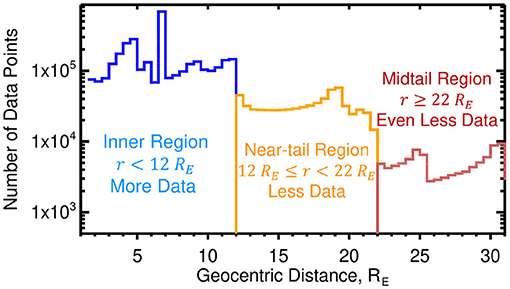
Figure 1. Radial distribution of magnetometer data. A histogram showing the radial distribution of the magnetometer database using r = 0.5R_E radial bins. The database covers three distinct regions with differing numbers of data points: the inner (blue), near-tail (orange), and midtail (brownish-red) regions.

The Near-tail Region 12R_E ≤ r ≤ 22R_E has a noticeable drop in data coverage, as only two outer THEMIS probes were ever located here and only for about 2 years before then were moved into a lunar orbit becoming the ARTEMIS mission [59]. With an apogee of r ≈ 18R_E, the Cluster mission (four probes) helps populate this region, however, as a polar orbiting spacecraft, they spent a limited amount of time in the equatorial region.

Beyond 22R_E the data density drops off by nearly an order of magnitude as the only spacecraft in the database that spent a considerable time in this region was Geotail. The near-earth reconnection sites are expected to be located here [60]. This motivated including the 2016–2017 MMS data. With an apogee of r ~ 26R_E, it nearly doubled the amount of data between 22R_E ≤ r ≤ 26R_E. The only other spacecraft included in the database is IMP-8, however, it comprises a relatively small amount of the total dataset.

For each time step, the model is fit to the identified subset of magnetometer data by minimizing the root mean square of the difference between the model B^(mod) and the observed B^{j, obs} magnetic field vectors:

$\begin{array}{ll}{M}_{err}^{(NN)}=\sqrt{{\displaystyle \sum _{j\in S_{NN}}}{\displaystyle \sum _{i=x,y,z}}{w}_j{w}_{(0)}(r){\left[B_i^{(mod)}({\text{r}}^{(j)})-B_i^{j,obs}\right]}^2},& (9)\end{array}$

where S_NN is the number of data points in the magnetometer subset identified through the kNN technique. The model is evaluated at the spacecraft's position r. Two weight factors are incorporated into the objective function, one based on the data point's position in physical space w₍₀₎(r) and the other on its position in state-space w_j. The first, w₍₀₎(r), lowers the weight factor in regions of the magnetosphere with a high density of data and was introduced to limit the bias of the fit toward these regions, in particular, to decrease the influence of the GOES satellites which are all located at the same radial distance [21]. The other weighting factor w_j gives higher weights toward observations which correspond to NNs that are closer to the moment of interest in state-space and will be described in the next section. The set of non-linear parameters (D, D_TCS, κ_R1, κ_R2, R_H, G, and TW) are found by minimizing Equation (9) using the downhill simplex method [61], while the amplitude coefficients are solved using the singular value decomposition (SVD) pseudo-inversion method [62, 63] also by minimizing (9).

2.4. Model Resolution Dilemma

The kNN approach has shortcomings caused by both the disparate density of NNs in the state-space and also the disparate density of magnetometer observations within the magnetosphere. The cause of the former is that, like many observed outputs of complex natural systems, geomagnetic indices, such as the substorm (AL) and storm (e.g., Sym-H^*) indices, tend to follow lognormal distributions [64–66], meaning the distribution contains many weaker storms and substorms than stronger ones. The result is that the NNs are inhomogeneous within the state-space, biasing the kNN method toward weaker events, which is especially problematic for strong and extreme events. Decreasing K_NN helps resolve this problem but introduces another, overfitting. This problem was addressed in a pair of studies [35, 36] that demonstrated introducing a simple distance-weighting of the NNs could significantly reduce this bias while keeping the K_NN large enough to temper overfitting. The NNs are weighted using a Gaussian function of the form

$\begin{array}{ll}{w}_j=exp\left[-{\left(R_q^{(j)}/\sigma R_{NN}\right)}^2/2\right],& (10)\end{array}$

where R_q is the distance of each NN to the query point and R_NN is the radius of the NN n-sphere, which is the maximum R_q (the distance between the query point and the most distant NN). σ determines the narrowness of the Gaussian and the value of σ = 0.3 is utilized here. These weights are then attached to the magnetometer datapoints when the model is fit by minimizing Equation (9). However, the second problem that was left unaddressed in those studies was the disparate data density in real/physical space caused by the distribution of spacecraft as shown in Figure 1.

The choice of K_NN in the kNN approach is a tradeoff. A small number (K_NN ~ 1) is akin to event-oriented modeling but requires a similarly small number of degrees of freedom in the model, i.e., the combined number of scaling coefficients a_i and non-linear parameters β_j are also on the order of unity [25, 26]. Increasing K_NN permits more complex models with a larger number of degrees of freedom (more a_is and β_js), but when K_NN approaches the size of the database the model becomes a universal statistical fit similar to classical Tsyganenko models (e.g., [17, 19, 38]) with a weaker sensitivity to storm and substorm phases. During the development of the SST19 model, it was found that an equatorial model resolution of (M, N) = (6, 8) using K_NN = 32, 000 was sufficient for reconstructing the primary substorm configuration of the magnetotail while avoiding overfitting. For this study, the model described in section 2 using these SST19 values of (M, N) = (6, 8) and K_NN = 32, 000 will be labeled the Tail Model. Figure 2 (right panels) displays the Tail Model's 2D equatorial distributions of the magnetic, electric current, and pressure fields during the late growth phase of a substorm (described below in section 3.2). For the sake of simplicity, these equatorial slices ignore dipole tilt and twisting effects, thus aligning the magnetic equator with the equatorial plane. Current densities are determined by numerically evaluating Ampere's law $\text{j}=\frac{1}{{\mu }_0}\nabla \times \text{B}$. The pressure is computed by integrating j × B radially inward starting at the boundary r = 10R_E in the manner detailed in [35]:

$\begin{array}{ll}P(r)-P(r_0)={\displaystyle \underset{r=10R_E}{\overset{r}{\int }}}{\left[-\text{j}\times \text{B}\right]}_r\text{d}{r}^{\prime }& (11)\end{array}$

where the boundary pressure P(r₀) is assumed to be small and set to zero. Figure 2 demonstrates how the Tail Model performs well throughout the near-tail and midtail regions and thus is suitable for substorm studies. However, within the predominant THEMIS inner probes apogee (gray circle) the current densities appear underresolved. Specifically, the eastward currents are almost entirely absent (Figure 2D). Without an eastward current, the integrand [−j × B]_r monotonically increases earthward from the boundary r = 10R_E meaning the pressure also increases monotonically. Thus, the location of the pressure peak is absent and the pressure radial gradients are also missing (Figure 2F).

FIGURE 2

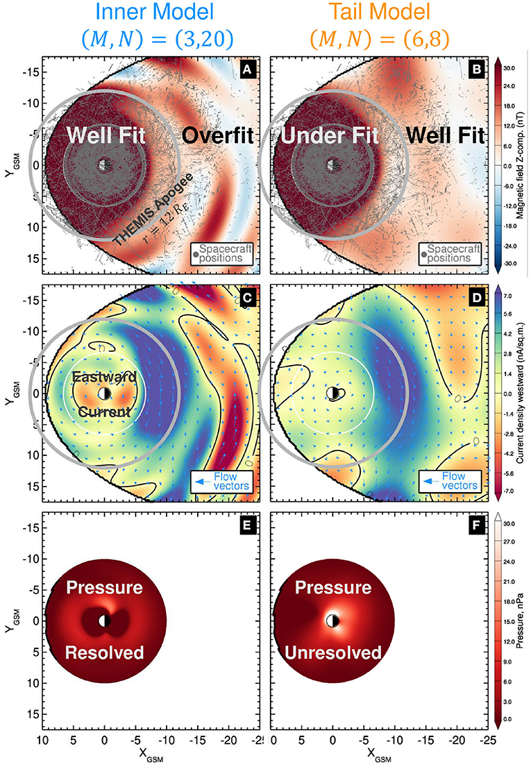
Figure 2. The model resolution dilemma. 2D equatorial distributions of the late growth phase (11:25) of a substorm on 8 March 2009 using two different equatorial resolutions. (A,B) The equatorial distribution of the total modeled magnetic field. The location of the spacecraft magnetic field observations used to fit the model are overplotted with gray dots. The predominant apogee of the inner probes of the THEMIS mission r = 12R_E is represented by the gray circle. (B,C) The equatorial distribution of the current density. The overplotted arrows show the direction and magnitude of the current density vectors. (E,F) The equatorial distribution of the pressure computed by integrating j × B according to Equation (11). The Inner Model is used for the left hand panels (A,C,E) which is fit using an equatorial resolution of (M, N) = (3, 20). It performs well in the inner region but overfits the near-tail region. The Tail Model is used for the right hand panels (B,D,F) which is fit using an equatorial resolution of (M, N) = (6, 8). It performs well in the near-tail region but under resolves the inner region.

In contrast, storm-time empirical reconstructions of the inner region (r ≤ 12R_E) were able to reconstruct the eastward current and thus the pressure, its peak, and gradient with the essential difference in the configuration of these models being a larger radial expansion number N = 20 used in the equatorial current module [33, 35, 36, 67]. Furthermore, the inclusion of the TCS particularly helped in resolving the eastward current when the storm state of the magnetosphere was relatively quiet [35]. However, the addition of the TCS in the model resulted in reconstructed pressures with rather large azimuthal gradients. This was mitigated by halving their number from M = 6 to M = 3, yielding a smoother pressure distribution, resulting in an equatorial resolution of (M, N) = (3, 20). Thus, the Inner Model is defined using this resolution of (M, N) = (3, 20) with all other model configurations being the same as the Tail Model. The analogous reconstruction of the substorm growth phase using this Inner Model are plotted in the left-hand panels of Figure 2 demonstrating that it does indeed capture the eastward ring current (Figure 2C) and appropriate pressure distributions (Figure 2E). However, the magnetic and current density reconstructions now contain numerous artifacts throughout the near-tail region (Figures 2A,C) indicating overfitting there.

Herein lies the dilemma; no single resolution is capable of adequately reconstructing both the inner and near-tail regions using K_NN = 32, 000 (the amount required to reconstruct the near-tail). Higher equatorial resolutions are necessary to describe the eastward current systems but will overfit the near-tail due to the lesser amount of data there and vice versa; lower equatorial resolutions perform well in the near-tail but miss the eastward currents in the inner region. This results in a bifurcation of models: the Inner Model (higher resolution) is suitable for storm spatial-scale reconstructions and the Tail Model (lower resolution) is applicable to substorm scales. A potential solution is to dramatically increase the value of K_NN, however, due to the disparate density of data in state-space, this would weaken the model's sensitivity to the event of interest and would begin to resemble statistical modeling instead of the DM approach sought. A simple solution would utilize a piecewise field, that is, to evaluate the Inner Model in the inner magnetosphere region and the Tail Model in the near-tail region. However, the equatorial current sheet described by Equations (1) and (2) ensures a divergenceless B and j fields. Such a piecewise field would introduce discontinuities which would violate these conditions and would also introduce infinitely thin current sheets. The resultant question is how to transition between these regions in a way that maintains ∇ · B = 0 and ∇ · j = 0? The next section 3 presents a simple resolution to this dilemma that smoothly transitions between the two regions while maintaining divergenceless fields.

It must be stressed that this resolution dilemma is not just a technical issue related to the sparse data distribution in space and the need to improve it is some regions. It reflects different physics processes associated with magnetic storms in the inner magnetosphere and substorms that reconfigure the magnetotail and create new FAC systems. In the earlier DM algorithms both storm and substorm descriptions used fleets of synthetic probes mined in the history of the magnetosphere. But these descriptions did not exchange the information gained from inner and outer magnetosphere description. So the fitting challenge resembles the first-principles model problem of the concurrent description of magnetic storms using the dedicated ring current models [68–70] and global MHD models [71–73] that often properly describe the outer magnetosphere. The resolution of that physics-based problem is similarly offered in the form of coupled models [74–77], when the information on the plasma conditions at some boundary separating inner and outer magnetosphere is transferred from MHD to ring current models. At the same time, the latter are used to adjust the equation of state in MHD taking storm effects into account.

3. Merged Model

3.1. Merged Model Algorithm

In this section, a simple method for concurrent reconstruction of both substorm and storm spatial scales is proposed, thus addressing the model resolution dilemma described above. The general approach is to introduce a third model, termed here the Merged Model, constructed using an equatorial resolution of (M, N) = (6, 20), the lowest common resolution between the Tail (M, N) = (6, 8) and Inner (M, N) = (3, 20) models. However, instead of fitting the Merged Model to actual spacecraft magnetometer data points, it is instead fit to virtual data, which are simulated by randomly sampling the equatorial regions of the Tail and Inner models outside and inside the merging boundary, respectively. Because the Tail and Inner models can be sampled at any location, the introduction of these virtual datapoints allows the Merged Model to be fit with an arbitrary density of points. The result is a Merged model (given a proper distribution of virtual data points) that tends to reflect the Inner Model within the merging boundary and the Tail Model beyond it with a smooth transition between the two in the vicinity of the boundary. Also, because the Merged Model's equatorial field is still described by Equations (1) and (2), by construction ∇ · B = 0 and ∇ · j = 0 is ensured.

For simplicity, a cylindrical boundary is used identified by the merging radius R_M. Initially, R_M was defined to be commensurate with the demarcation between the inner and near-tail regions as characterized by the predominant THEMIS inner probes apogee (r = 12R_E from Figure 1), though, this yielded unsatisfying results. Figure 3 shows 1D plots of the external magnetic field $B_z^{ext}$ (Figures 3A,B) and the westward component of the current density j_w = −j_ϕ (Figures 3C,D) for the Inner (blue lines) and Tail (orange lines) models along the X axis. Two different moments are shown corresponding to the late growth (left panels) and expansion (right panels) phases, respectively. Ideally, there would exist a clear boundary where $B_z^{ext}$ and j_w from the two models intersect. Instead, the intersections (between the blue and orange lines) vary between ~6R_E–10R_E. This justifies moving R_M earthward of the THEMIS apogee of 12R_E. Ultimately, the center of this region, that is, a cylindrical radius of R_M = 8R_E was chosen, which will be used as a constant merging boundary throughout the rest of the study. Although this is a rather arbitrary value, as shown below, this choice of R_M enables the Merged Model to fully capture the deep $B_z^{IMF}$ minimums and eastward currents of the Inner Model while also reconstructing the substorm scale features of the SST19 and Tail Model. The merging algorithm can be enhanced in future studies by incorporating a dynamical merging boundary that minimizes the differences of $B_z^{ext}$ and j_w between the Tail and Inner models. The use of elliptic cylindrical boundaries should also be pursued as Figure 3 indicates that day-night asymmetries exist in the optimal merging location.

FIGURE 3

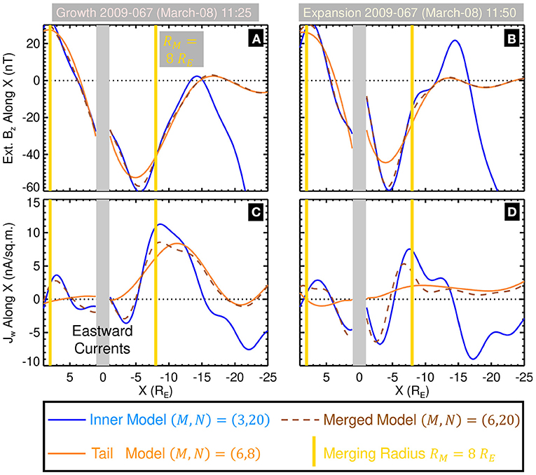
Figure 3. Determination of the merging radius. Line plots of (A,B) the z-component of the external magnetic field $B_z^{ext}$ and (C,D) the westward component of the current density j_w = −j_ϕ along the x axis for the Inner (blue line), Tail (orange line), and Merged (dashed brown line) for two different moments in time corresponding to the growth phase (left panels) and expansion phase (right panels) of the 8 March 2009 substorm. The location of the chosen merging radius R_M = 8R_E is denoted by the vertical yellow lines.

To create the Merged Model, the non-linear parameters (D, D_TCS, κ_R1, κ_R2, R_H, G, and TW) are taken to be the average of their values from the Inner and Tail models and are not included in the fit; while the linear amplitude coefficients for the equatorial and FAC systems are fit in the manner described before, that is by using the SVD least-squares method to minimize Equation (9). However, instead of using real magnetometer data points, the $B_i^{j,obs}$ terms in (9) are populated with virtual measurements constructed by evaluating the Inner and Tail models. The Inner Model was randomly sampled to achieve a data point density of $1{R_E}^{-3}$ within the cylindrical volume 1.1R_E ≤ r ≤ R_M, −6R_E ≤ z ≤ +6R_E. The value of ±6R_E was chosen as it is twice the typical value of the thick current sheet half thickness D ≈ 3R_E. Meanwhile, given the lower radial resolution of the Tail Model, it was only sampled at a data point density of $0.2{R_E}^{-3}$ within the cylindrical volume R_M ≤ r ≤ 31R_E, −6R_E ≤ z ≤ +6R_E. While this worked well for resolving the thick current sheet, due to the small height scale size of the TCS, additional samples were needed from the region −1R_E ≤ z ≤ +1R_E, where ±1R_E is twice the typical TCS half-thickness D_TCS ≈ 0.5R_E now using six times the densities from before, $6{R_E}^{-3}$ and $1.2{R_E}^{-3}$ for the Inner Model and Tail Model, respectively. The reason for using a random distribution of points in contrast to a regular grid, is that fitting a regular grid of points with a magnetic field described by the regular expansion in Equation (1) may introduce artifacts caused by the model aligning to the grid instead of the underlying magnetic field distribution. In total, 18, 260 virtual spacecraft datapoints were included in fitting the amplitude coefficients of the Merged Model.

The output of the Merged Model is overplotted in Figure 3 as brown dashed lines. Earthward of R_M the Merged Model generally tracks the Inner Model (blue line) including the deep minimums in $B_Z^{ext}$ (Figures 3A,B) and the eastward currents (Figures 3C,D), both of which are key characteristics needed to reconstruct the storm-time dynamics of the inner magnetosphere [33]. Tailward of R_M the Merged Model closely matches the Tail Model (orange line). This indicates that the Merged Model should also reconstruct the primary substorm scale features, such as the thinning and stretching of the magnetotail during the growth phase and its rapid dipolarization during the expansion phase, as will be shown in the next section 3.2. In the ~±2R_E region bounding R_M, the Merged Model smoothly transitions between the Inner and Tail models.

In order to qualitatively compare the Merged Model to the Inner and Tail models, 2D equatorial slices of the magnetic and current density fields are plotted for the late growth phase in Figure 4. Inside the merging radius R_M = 8R_E (yellow circles) the Merged Model qualitatively resembles the Inner Model, and importantly for the evaluation of the pressure, resolves the eastward currents (orangish-red region r ≲ 5R_E in Figures 4D,F). Outside of the R_M, the Merged Model (Figures 4C,F) is nearly indistinguishable from the Tail Model (Figures 4B,E). Notably, the Merged Model resolves the B_z minimum formation in the tail at 10R_E ≲ r ≲ 13R_E and the enhancement of the cross tail current at 7R_E ≲ r ≲ 16R_E. The distribution of the virtual spacecraft projected into the equatorial plane used to fit the Merged Model is overplotted in Figure 4C, showing how random sampling of the other two models evenly fills in data gaps present in the near-tail and midtail regions, particularly beyond the Cluster apogee (r≥19R_E). A note, as can be seen in Figure 4, the Inner Model is now only being fit using data within the predominant THEMIS inner probes apogee of r ≤ 12R_E. Including data beyond this serves no purpose because the Inner Model is only being sampled within r ≤ R_M when creating the Merged Model and their inclusion may bias its reconstructions.

FIGURE 4

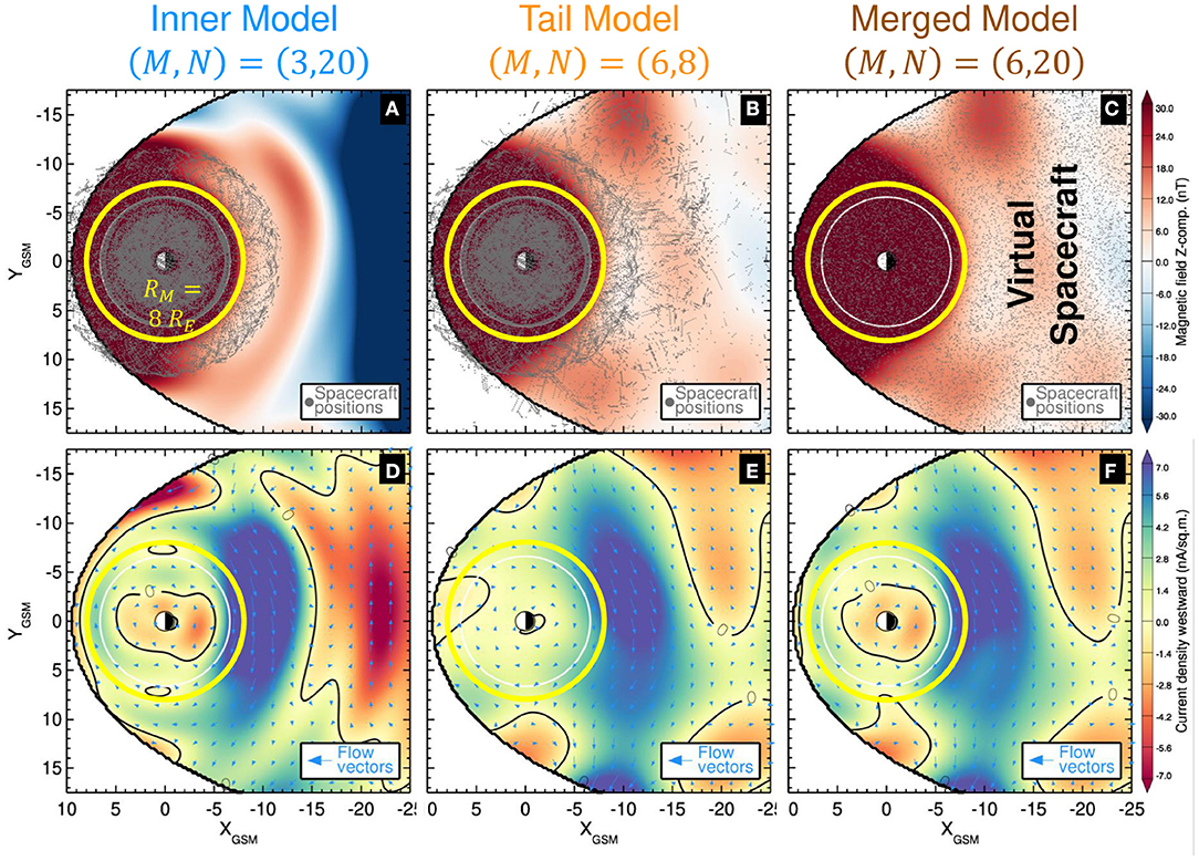
Figure 4. The Merged Model. 2D equatorial distributions of the late growth phase (11:25) of a substorm on 8 March 2009 using the merged equatorial resolution model compared to the Inner and Tail models. (A–C) The equatorial distribution of the total modeled magnetic field. The location of the spacecraft magnetic field observations (virtual for the Merged Model) used to fit the model are overplotted with gray dots. The merging radius R_M = 8R_E is represented by the yellow circle. (D–F) The equatorial distribution of the current density. The overplotted arrows show the direction and magnitude of the current density vectors. Note how the Merged Model resembles the Inner/Tail models inside/outside R_M.

The differences between the Inner/Tail and Merged models from the panels in Figure 4 are displayed in Figure 5. Within geosynchronous orbit, the differences between Inner and Merged models are relatively small (Figures 5A,C), with maximum values of B = 1.9 nT and j = 3.6 nA/sq.m and mean differences of B = 0.66 nT and j = 0.9 nA/sq.m. In this same region, the differences between the Tail and Merged models are about two to three times larger, with maximum values of B = 3.9 nT and j = 6.8 nA/sq.m and means of B = 1.8 nT and j = 2.5 nA/sq.m. The comparison between the Tail and Merged models shows negligible differences beyond ~10R_E (Figures 5B,D), while the equivalents for the InnerModel display large differences there. This confirms that the Merged Model largely mimics the Inner Model in the inner magnetosphere and the Tail Model in the near-tail. However, of interest are the differences in the vicinity of the merging boundary. Within the ±2R_E region bounding R_M, the mean differences are B ≈ 1 nT and j ≈ 2 nA/sq.m but show rather large maximum differences; B = 5 nT, j = 10 nA/sq.m for the Inner Model and B = 3 nT and j = 6.5 nA/sq.m for the Tail Model. The cause of this being the relatively large mismatch between the Inner and Tail models as is evident in the Figures 3, 4. This further supports additional investigation into a more optimal merging boundary in future works.

FIGURE 5

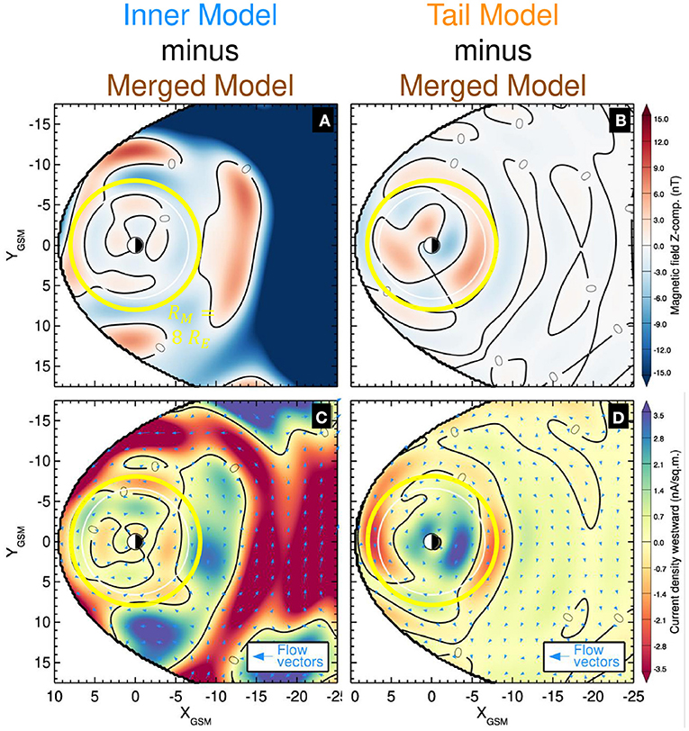
Figure 5. The Merged Model differences. The difference between Inner/Tail and the Merged Model 2D equatorial distributions from Figure 4. The format is the same as Figure 4 but the range on the color bars has been halved to emphasize the differences.

3.2. Merged Model Reconstruction of 8 March 2009 Substorms

Global reconstructions for the second 8 March 2009 substorm are displayed in Figures 6, 7, the first corresponding to the late growth phase at approximately the time of the substorm onset and the second is 25 min later during the expansion phase as indicated by the AL index (Figure 6a). These reconstructions highly resemble the reconstructions of the same event using the SST model [15] (Figures 3, 4 from that work). This confirms that the Merged Model is mostly analogous to the SST19 model throughout the near-tail region as was expected from the analysis shown in Figures 3, 4. However, the Merged Model now reconstructs the eastward currents as can be seen near the planet in Figures 6e, 7e.

FIGURE 6

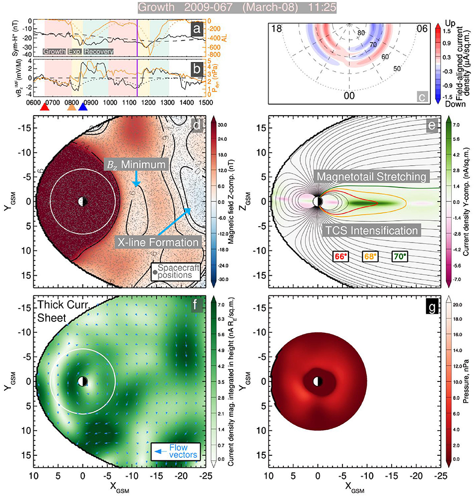
Figure 6. The merged resolution model's reconstruction of the late growth phase of the 8 March 2009 substorm. (a) Geomagnetic indices: the pressure-corrected storm index Sym-H^* and substorm index AL in solid black and orange lines, respectively. Their smoothed values $G_1^{(sst)}(t)=\langle {Sym\text{-}H}^{*}|$ and $G_3^{(sst)}(t)=\langle AL|$ are shown by dashed black and dotted orange lines, respectively. (b) Solar wind parameters: the electric field $v{B}_z^{IMF}$ and dynamic pressure P_dyn in solid black and orange lines, respectively, with $G_5^{(sst)}(t)=\langle v{B}_s^{IMF}|$ shown as the dotted black line. The vertical purple lines in (a,b) represent the moment in time. (c) The pattern of FACs flowing into (blue) and out of (red) the ionosphere. (d) The equatorial distribution of the total modeled magnetic field. The simulated magnetic field observations used to fit the model are overplotted with gray dots. (e) The meridional distribution of the Y component of the current density showing current flowing out of the page (green) and into the page (purple). Magnetic field lines originating from the ionosphere (ranging from 60 to 90° magnetic latitude with 2° steps), three of which are highlighted: 66° (red), 68° (yellow), and 70° (green). (f) The height integrated equatorial distribution of the thick current sheet's current density integrated from 0 ≤ Z ≤ 5R_E. The overplotted arrows show the direction and magnitude of the current density vectors. (g) The equatorial distribution of the pressure computed by integrating j × B according to Equation (11).

FIGURE 7

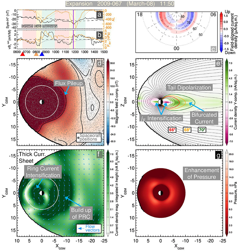
Figure 7. The merged resolution model's reconstruction of the expansion phase of the 8 March 2009 substorm. Panels are the same as Figure 6 except 25 min later.

During the growth phase, the magnetotail is stretched (Figure 6e), particularly in the region between ~8R_E and 15R_E corresponding to the B_z minimum region (Figure 6d). The TCS is especially intense on the night side in this same region (Figure 6e). The 66 and 68° field lines cross the magnetic equator at 12R_E and 18R_E, respectively while the 68° line is open. The height integrated thick current sheet is plotted (Figure 6f) as it is a better proxy for the content of the ring current compared to the equatorial slice of the current density (as is shown in Figures 2, 4) because the current density of the TCS tends to be the dominant source of current density along the magnetic equator. This panel shows a modest westward ring current within geosynchronous orbit r ≲ 6.6R_E as well as a strong outflow to the magnetopause at the dusk terminator. The pressure during the growth phase is relatively azimuthally symmetric, with a pressure peak at 4–5R_E.

During the expansion phase, which takes only 25 min, the global configuration of the magnetosphere is drastically altered (Figure 7). The magnetotail becomes much more dipolar. The 66° field line (Figure 7e) now crosses the magnetic equator at 7.5R_E (compared to 12R_E in the growth phase) and the 68° line crosses at 10R_E (compared to 18R_E). The previously open 70° field line now crosses at 14R_E, indicating the conversion of open to closed flux presumably from reconnection. This dipolarization is congruous with the formation of the magnetic flux pileup in this region (Figure 7d). There is a strong enhancement of an westwardly directed thick current all across the night side taking the appearance of a PRC (Figure 7f). However, the SST19 analysis [15] along with magnetohydrodynamic (MHD) simulations [78] indicated that the enhancement of this PRC is associated with closure through the substorm current wedge. The substorm current wedge manifests as a eastwardly directed TCS in the vicinity of the magnetic equator, but its closure out of the plane is via a westwardly directed thick current, some of which closes through the ionosphere as R2 currents. Another point of agreement between the Merged Model and the SST19 model is the strengthening of the dayside thick current sheet within geosynchronous orbit (r ≤ 6.6R_E), which was interpreted as an intensification of the symmetric ring current.

3.3. Merged Picture vs. Earlier Substorm Reconstruction

The quantitative analysis performed using the SST19 model for the 8 March 2009 substorms [15] is now recreated using the Merged Model, in particular their Figure 6 is recreated and is shown as Figure 8. Compared to that substorm-focused reconstruction, the Merged Model reveals more profound variations of the R2 FAC amplitudes (Figure 8d), stronger buildups and decays of the TCS integrated current (orange line in Figure 8f) with significant negative values implying bifurcated current structures. One such bifurcated current structure is well seen in the meridional current distribution presented in Figure 7e.

FIGURE 8

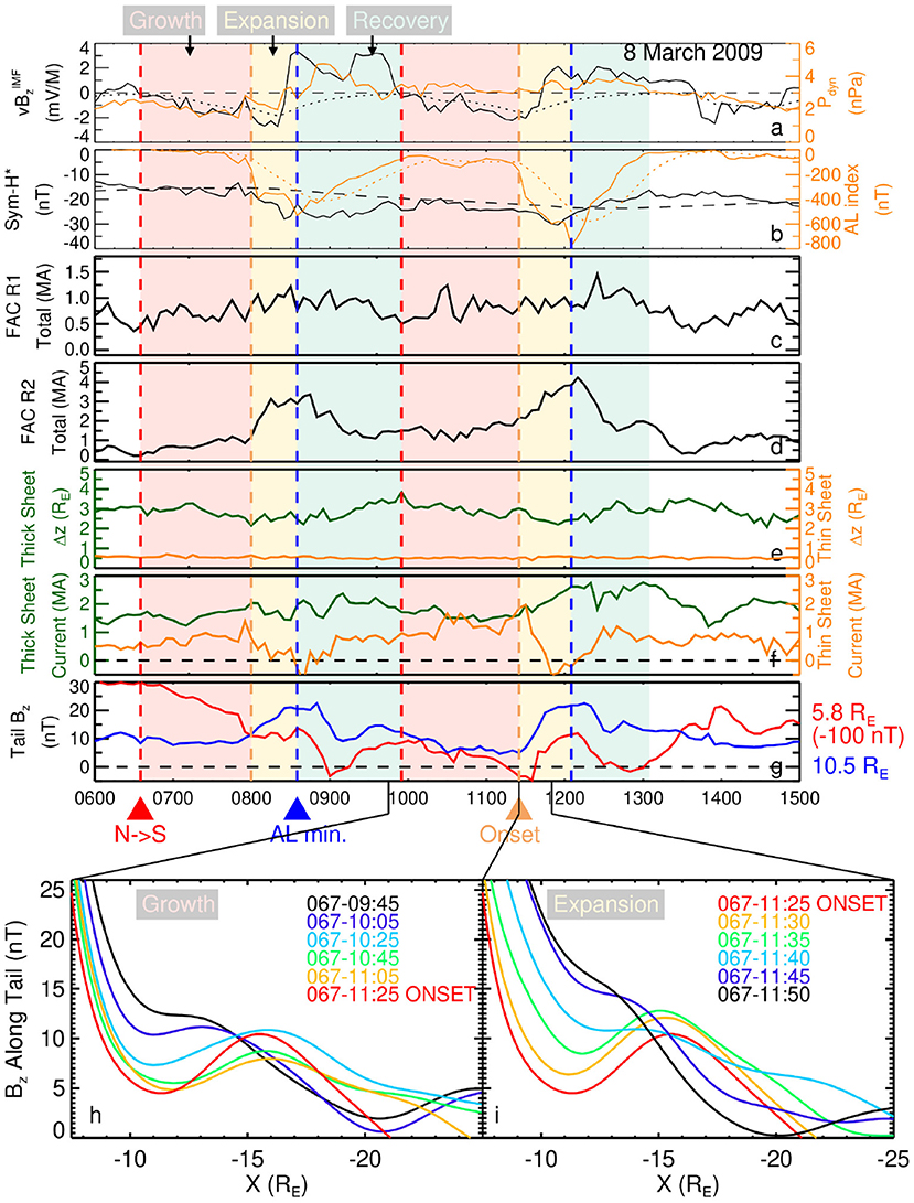
Figure 8. The Merged Model quantitative analysis. (a,b) Geomagnetic indices and solar wind parameters in a format similar to Figures 6a,b. (c,d) The root mean square of the FAC amplitude coefficients for the R1 and R2 FAC modules, respectively. (e) The values of the current sheet half thicknesses for the thick sheet (green line) and TCS (orange line), i.e., D and D_TCS from Equation (2). (f) A measurement of the amount of current contained in the dayside SRC (green line) and nightside TCS (orange line). The SRC current (green line) is computed by integrating the dayside westward current density of the thick current sheet module flowing within geosynchronous orbit 1.0R_E ≤ x ≤ 6.616R_E and z = ±5R_E. The TCS current (orange line) is computed by integrating the nightside westward current density of the TCS module flowing within the rectangle −16R_E ≤ r ≤ −6R_E and z = ±1.0R_E. (g) The z-component of the total magnetic field B_z sampled at x = −5.8R_E (red line) and x = −10.5R_E (blue line). (h,i) The z-component of the total magnetic field B_z along the nightside x-axis at different times during the growth and expansion phases.

The merged resolution picture reveals stronger variations of the B_z magnetic field at the Van Allen Probes inner probes apogee (red line in Figure 8g). These stronger variations reflect the impact of distance-weighting the NNs along with a better resolution of the inner magnetosphere region resulting eventually in the resolution of the eastward current and the plasma pressure shown in Figures 6g, 7g. At the same time, it resolves the formation of the near-Earth X-line around the substorm onset (red and orange lines in Figures 8h,i), which is also seen in Figure 6d. Its resolution becomes possible not only due to the solved overfitting problem for the tail region, but also due to the use of the MMS data and the distance-weighted kNN algorithm as is elaborated in detail in [30].

The comparison also reveals some pitfalls of the present merging algorithm. In particular, unlike the SST19 model, the merged resolution model no longer has a clear correlation between the substorm phase and the amplitude of the R1 currents (Figure 8c). The probable explanation, is that because the R1 currents do not close through the equatorial plane (in contrast to the R2 currents), relatively few of the virtual spacecraft points sample them. To rectify this in future reconstructions using the Merged Model, the amplitude coefficients for the FAC systems should be set in a similar fashion to the non-linear parameters and not included in the fit. This is reasonable since the focus of the merged modeling approach is to combine two models with different equatorial resolutions.

The primary enhancement of this Merged Model over the previous SST19 model is the resolution of the pressure in the inner magnetosphere. In order to quantify the change in pressure during the course of a substorm, the 2D pressure distributions from Figures 6g, 7g are averaged over all local times for a given radial distance r. The resultant average pressures 〈P〉 are plotted as a function of radial distance r for the second 8 March 2009 substorm in Figures 9D,E for several moments during the growth and expansion phases (the solar wind values and geomagnetic indices are included for context in Figures 9A,B). During the growth phase, the average pressure stays relatively stable, with a max value between ~5–6 nPa located at 4.25–4.5R_E. In contrast, during the expansion phase 〈P〉 rapidly increases reaching values as high as 10 nPa while the location of the peak stays relatively stable. The time series for 〈P〉 at 4.5R_E is then plotted in Figure 9C for both substorms, showing that during quiet and growth phases the pressure is stable and low but then rapidly increases during the expansion phase. 〈P〉 then decreases during the recovery phase, although for the second stronger substorm, it does not return to the nominal value until more than 3 h after the substorm onset. Such an enhancement of inner magnetosphere pressure is consistent with in-situ observations [12] of particle injections as well as statistical analyses [13] of substorm expansion phases.

FIGURE 9

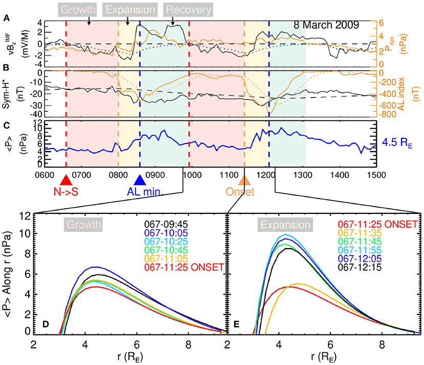
Figure 9. Substorm enhancement of pressure. (A,B) Geomagnetic indices and solar wind parameters in a format similar to Figures 6a,b. (C) The value of the pressure averaged over all local times at r = 4.5R_E. (D,E) The averaged pressure vs. radial distance at different times during the growth and expansion phases.

3.4. Uncertainty Quantification

An important aspect of empirical model development is its validation via comparison of the model output to the data that went into its construction. In this section, three different analyses are performed to test the model's fidelity. First, the DM approach is analyzed to ensure that the identified NNs characterize the 8 March 2009 substorm event and next the in-situ spacecraft magnetometer data is compared to the reconstructed field. Lastly, the three different models are statistically cross-validated using ~28 days of model reconstructions to quantitatively assess the model error as a function of activity mode and radial distance.

The DM approach assumes that there are enough similar events in the state-space that the NNs collectively match the event of interest. This assumption can be tested by using the state-space analysis performed in earlier studies [30, 35, 67] in which the time evolution of the state-space components G_i(t) (the binning parameters) for the studied event are compared to the mean of those parameters over the NNs $G_i^{(NN)}(t)$. Ideally, $G_i^{(NN)}(t)$ should match G_i(t).

Figure 10 shows the evolution of the five components of the combined storm and substorm state-space (black lines) during the two 8 March 2009 substorms corresponding to the quantities described by Equations (4)–(8). Panels a, c, and e demonstrate how the integral convolutions act to smooth the original data (pink lines). It should be stressed that the smoothing windows are asymmetric in time, that is, they are only computed over previous and not future data points [note the zeros on the upper bounds in the integrals (4)–(8)]. This was introduced to prevent the smoothed parameters from changing prior to the start of an event [48]. For example, without this asymmetry, the model would begin reconstructing storm activity prior to the arrival of the southward IMF in the solar wind. This causes the smoothed values to lag the original (black lines lag behind the pink lines). However, as demonstrated by Figure 8, this is not problematic as the time lag is universally applied over the entire dataset. Note how the modeled magnetic field (Figure 8g) and model parameters (Figures 8d–f) are still largely correlated with the original value of AL (Figure 8a solid orange line) and not its smoothed value (dotted orange line).

FIGURE 10

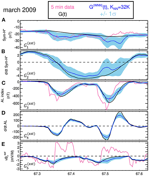
Figure 10. Storm-substorm 5D state-space. (A–E) Time series of the five individual components (black lines) of the state-space used to characterize the combined storm and substorm state of the magnetosphere as defined in Equations (4)–(8) during the two 8 March 2009 substorms. Their standardized values are used to find K_NN = 32, 000 nearest-neighbors (NNs) in the entire state-space. The weighted mean of the 32, 000 NNs are overplotted by the blue lines. The weighted standard deviation of the NNs is then overplotted by showing ±1σ as the light blue envelopes around the weighted NN means.

The weighted average of the state-space vector over the closest K_NN = 32, 000 NNs is shown by the blue lines: ${\text{G}}^{(WNN)}=\sum _j^{K_{NN}}{w}_j{\text{G}}_j/\sum _j^{K_{NN}}{w}_j$, where the weight factor w_j is computed using the Gaussian distance weighting from Equation (10). In a similar manner, the weighted standard deviations of these parameters over the set of NNs is also computed and the ±1σ values are indicated by light blue envelopes that surround G^(WNN) (blue line) in Figure 10. Overall, G^(WNN) largely stays within 1σ for the event of interest (black line).

The most notable inconsistencies appear in 〈Sym-H^*| and D〈Sym-H^*|, which is a result of mixing parameters of different smoothing scales. Sym-H^* and its derivative are smoothed over storm time frames of Π_st = 12 h while the AL equivalents are instead smoothed over substorm scales Π_sst = 2 h. This also demonstrates that the pressure-corrected storm indices contain contributions from substorm current systems and is not representative of just a pure ring current as has been discussed in previous studies [79, 80]. Other deviations appear in particularly when 〈AL| it reaches its minimum. The cause of this is the inhomogeneity of the datapoints in state-space as has been extensively discussed in earlier works [35, 36, 67]. This biases the DM approach toward weaker events as they occur more frequently which is only exacerbated as the events of interest become more extreme [36]. Distance-weighting the NNs can drastically mitigate this issue [35], although, as is shown in the second substorm, it does not entirely correct it. For instance, the minimum value for the second substorm is 〈AL| = −576 nT while the mean over the NNs is only 〈AL|^(WNN) = −478 nT.

Next, the reconstructed magnetic field of the Merged Model is compared to the available in-situ magnetic field measurements from the THEMIS and GOES satellites (Figure 11). For this event, all five THEMIS probes are located in the magnetotail, with probes A, D, and E being in a similar orbital configuration situated at about post-midnight and r ≈ 12R_E, while probes B and C are at ~21 MLT with r ≈ 25 and 16R_E, respectively. As the magnetotail current sheet thins, less magnetic flux threads through it resulting in a decrease in B_z (e.g., [81]), as is observed by all five THEMIS probes during the growth phases, with B_z approaching values of B_z ~ 1 nT prior to substorm onset (panels b, e, h, k, and n; black lines). The model captures these thinning signatures for the inner probes A, D, and E (panels b, k, and n; brown lines) as their location places them within the B_z minimum and TCS region as was shown in Figures 6d,e. The model underestimates the thinning, as the B_z values only reach B_z ~ 4 nT during the growth phases. One explanation is that the $\langle v{B}_s^{IMF}|$ parameter is a suboptimal proxy for the development of the TCS in the magnetotail while another is that the DM approach smears the singularly thin nature of the TCS effectively making it thicker than in reality.

FIGURE 11

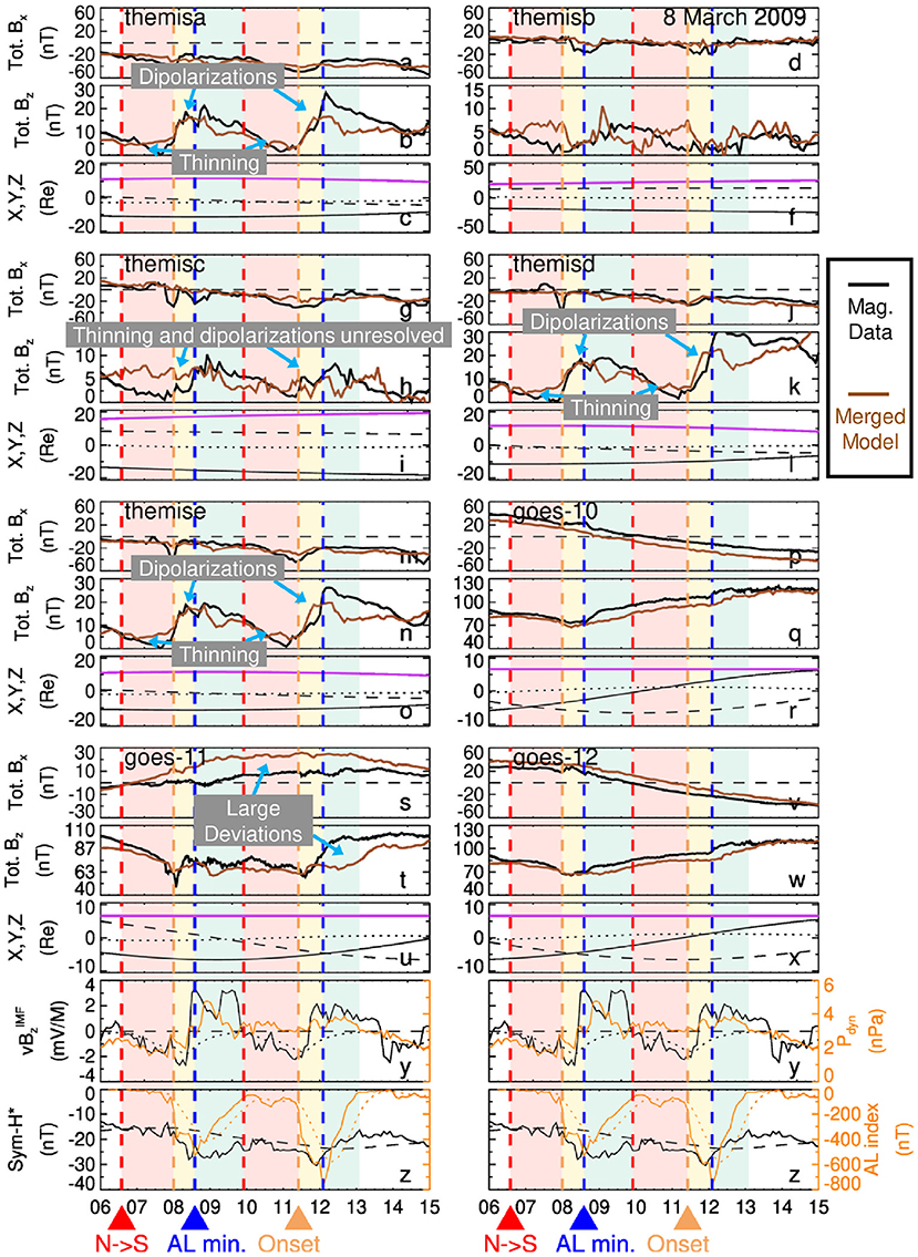
Figure 11. In-situ validation of the Merged Model. The comparison between the THEMIS and GOES magnetometer data and the Merged Model reconstruction of the 8 March 2009 substorms. (a,b) The x and z components of the total magnetic field B_tot observed by the THEMIS-A magnetometer (black line) averaged to 5 min resolution compared to the Merged Model evaluated at the spacecraft location (brown line) in the GSM coordinate system. (c) The THEMIS-A ephemeris in GSM coordinates with the x, y, z, and r components in solid, dashed, dotted, and purple lines, respectively. (d–x) The same as (a–c) except now for the other four THEMIS and three GOES satellites. (y,z) Geomagnetic indices and solar wind parameters in format similar to previous figures.

Following substorm onset and throughout the expansion phase, magnetic flux is transported earthward accumulating in the near-tail region and enhancing the value of B_z there (e.g., [82]), leading to a more dipolar magnetic field configuration. The three inner probes observe this dipolarization as a ~20 nT increase in B_z for the first substorm and a ~30 nT increase for the second (panels b, k, n; black lines). As was shown in Figure 7d, the model reconstructs this flux pileup across the whole nightside magnetotail to a distance of r ≈ 16R_E. The in-situ validation demonstrates that the model nicely captures these B_z increases for the inner probes (panels b, k, n; black lines). While the model effectively captures the magnitude of the flux enhancement for the first substorm, it underestimates it for the second. This is not unexpected, as the state-space analysis shown in Figure 10 demonstrated the DM approach underestimated the intensity of the second substorm (Figure 10c).

However, the model misses the TCS formation and the dipolarizations at the locations of outer probes B and C (Figures 11e,h) which are further down tail and whose MLTs are significantly away from midnight. Further, while the model displays good consistency with the GOES-10 and 12 magnetometers (Figures 11p,q,v,w), there are quite large deviations for GOES-11 (Figure 11t). This particular pair of substorms appears quite global in nature, showing signs of current sheet thinning as far as r ~ 20R_E down tail at 21 MLT and large dipolarizations at geosynchronous orbit at 3 MLT. While the AL index is a good indicator of the overall substorm intensity, it has its limitations. Firstly, it is derived from a rather small (10–12) number of magnetometer stations [44] and secondly, it yields no information about the local time configuration of the substorm currents [83]. As such, the DM approach will tend to reconstruct the typical substorm as is represented by the state-space parameters but will have no specific insight into the event's MLT configuration. This may be the underlying cause of the deviations between the model and the THEMIS B and C as well as the GOES-11 satellites. Some of these issues might be addressed by using another substorm index constructed from a more robust collection of magnetometer stations, such as the SML index [84], which furthermore, is computed for differing local time bins [85].

Overall, these results largely mirror to the validation of the SST model as shown in [15] (their Figure 2). This is not unexpected as the Merged Model closely matches the Tail Model at these spacecraft's locations and given that the Tail Model is very similar to the SST19 model. A shortcoming of the spacecraft configuration for this particular event is that none of them are earthward of geosynchronous orbit and according to Figures 3, 4, the improvement of the Merged Model over the SST19 model should be most apparent in this region. This will be addressed by a quantitative statistical analysis next.

In order to preform a quantitative uncertainty estimate the three models are cross-validated. In this technique, a subset of the data is reserved, that is it is not included when the model is fit, and instead forms a validation dataset. Statistical analysis is then performed on the independent validation set, and because this set was not used while fitting the model, it represents an out-of-sample test.

For the purposes here, the validation set should include spacecraft which adequately cover both the inner magnetosphere and near tail regions while there is also storm and substorm activity. The year 2015 was chosen to be the validation time interval as both the Van Allen probes and the THEMIS missions were sampling the inner magnetosphere, while the Cluster and MMS missions observed the near-tail. Further, the maximum sunspot count of solar cycle 24 peaked in April of 2014, so solar activity was still quite high throughout 2015 resulting in an elevated occurrence of geomagnetic storms [86]. Thus, when performing the model cross-validation, the entirety of the spacecraft dataset for the year 2015 was excised from the magnetometer database when fitting the models. That is, only data from spacecraft missions spanning the years 1995–2014 and 2016–2018 are used during fitting, while only data from 2015 are used in this cross-validation. Owing to the computational expense needed to fit the model, it was not feasible in this study to model the entirety of the year 2015. Instead, only times corresponding to storm and substorm activity from the 3 months of June, September, and December were modeled. At least one strong storm (Dst≾−100 nT) occurred during each of these months, and their separation in time allowed the spacecraft to sample a range of different local times. The start of September corresponds to the beginning of the MMS primary science mission phase, and as such is when the MMS magnetometer data becomes available. Here, storm and substorm activity time intervals are defined as when 〈Sym-H^*| ≤ −50 nT or 〈AL| ≤ −300 nT. To ensure that broader portions of the storm main and recovery phases and substorm growth and recovery phases were also included, the time intervals were expanded by ±3 h and ±30 min, respectively. In total, the identified storm and substorm activity time intervals across these 3 months spans 673.5 h or about 28 days, corresponding to 8,046 model fits and ≈ 68, 000 spacecraft magnetic field observations when evaluated at a 5 min cadence. Here, the out-of-sample model error is quantified using the magnitude of the difference between the model evaluated at the spacecraft location and the observed magnetic field there:

$\begin{array}{ll}{ϵ}_i=\parallel {\text{B}}^{(mod)}({\text{r}}_i)-{\text{B}}_i^{obs}\parallel .& (12)\end{array}$

This quantity is similar to the model residuals which are key to its fitting, for example, as seen in the objective function (9), but without the weighting factors. They also have been the primary metric for testing empirical magnetic field model fidelity in previous studies (e.g., [87–89]). Specifically, the average magnitude of the difference between the model and observation $\langle ϵ\rangle =\frac{1}{N}\sum {ϵ}_i$ is reported in Table 1, where N is the number of samples.

TABLE 1

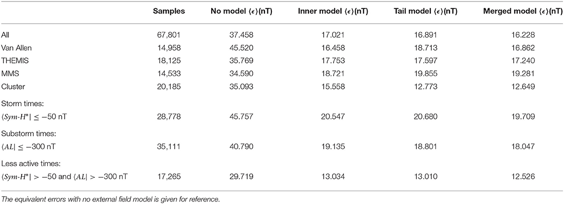
Table 1. Out-of-sample model errors 〈ϵ〉 for the Inner, Tail, and Merged Models for different spacecraft and activity levels.

The Inner Model performs marginally better for the Van Allen Probes data than the Tail Model as their orbit is entirely within the inner magnetosphere region. As Figures 3, 4 indicated, this marginal improvement in B is crucial for reconstructing the current density j which depends on the spatial derivatives of B. In contrast, the Tail Model has lower errors for the Cluster spacecraft which spends relatively little time in the inner equatorial magnetosphere. The THEMIS and MMS missions have similar errors for both models. All models display notably lower errors for the less active times, presumable because the global configuration is more regular. Substorm and storm performance is rather similar, although, the storms during the validation interval contain significant substorm activity based on the AL index. Further analysis could be performed to separate isolated, multiple, and storm-time substorms, and storm intervals with and without substorm activity. Importantly, the Merged Model generally matches the lower error of the two other models, statistically validating the algorithm discussed in 3.1. Indeed, the Merged Model has the smallest error across the entire validation set at 〈ϵ〉 = 16.228 nT. To put this in context, running the same model cross-validation for the commonly used T89 and T96 yields errors of 〈ϵ〉 = 20.006 and 21.777 nT, respectively, while using no model (B_ext = 0) gives is 37.458 nT.

To get a better indication of how the model errors change as a function of distance, the errors were collected into different radial bins (Δr = 0.25R_E when r < 12R_E; Δr = 1.0R_E when r > 12R_E, where Δr is the size of the bin) and for the different types of activity levels as are displayed in Figure 12. The Tail Model (orange lines) has significantly lower errors tailward of r = 12R_E compared to the Inner Model (blue lines), although, recall the later was not fit using data in this region, so it should not be expected to perform well here.

FIGURE 12

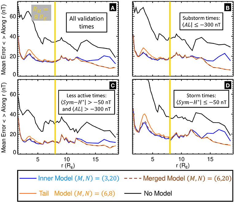
Figure 12. Mean model errors as a function of radius. The mean model errors 〈ϵ〉 computed in different radial bins for the Inner Model (blue lines), Tail Model (orange lines), and Merged Model (dashed brown lines). The errors when no model for B_ext is applied is shown for context using the black lines. The errors are further binned into different activity levels: (A) the entire validation set, (B) active substorm times 〈AL| ≤ −300 nT, (C) less active times 〈Sym-H^*| > −50 and 〈AL| > −300 nT, likely during the substorm and storm growth/main and recovery phases, and (D) active storm times 〈Sym-H^*| ≤ −50 nT.

Meanwhile, the Inner Model (blue lines) has lower errors within 3R_E ≤ r ≤ 6R_E, indicating that it does yield a more accurate reconstruction of the ring current region. However, errors are still relatively high here, particularly during storm times (Figure 12D), indicating the model still potentially underestimates the ring current intensity. One cause might be, given that there were several strong storms during this validation period (one storm reached a minimum Dst ≈ −200 nT while another hit Dst ≈ −150 nT), the aforementioned bias toward weaker events. Another, is that strong storms tend to have a complex morphology (e.g., [36]), and the multitude of mesoscale features can simply not be discerned with the DM approach. Also of note, the errors significantly increase earthward of r = 2.5R_E. This has been observed in in-situ comparisons in previous studies and was attributed to attitude uncertainty issues which make it difficult to distinguish between the internal and external fields (e.g., [35]) as the former is very large close to the planet. If these are indeed observational errors, then perhaps these datapoints earthward of r = 2.5R_E should be excised from the model database in future studies. Importantly for the context of this study, is that the errors of the Merged Model (dashed brown line) tend to follow the smaller of the other two across all radial bins. This confirms that the merging algorithm discussed in section 3.1 works as intended.

4. Discussion and Conclusion

In this paper we presented a new method of the empirical reconstruction of the magnetospheric substorms, which not only resolves the corresponding reconfiguration of the magnetotail but also resolves both westward and eastward currents in the inner magnetosphere that reflect the associated storm-type phenomena. In particular, it becomes possible to resolve and quantitatively evaluate the buildup of the storm-time plasma pressure, which was under-resolved in the previous substorm reconstructions [15]. The key to the solution of such a combined description of the inner magnetosphere is similar to the original kNN DM method [15, 22], where a swarm of many synthetic probes neighboring the event of interest in the binning parameter space was used. Here similar virtual probes were used and combined from different versions of the SST19 model focused on the inner magnetosphere and the tail region.

This merged resolution approach is also similar to coupled first-principles models of the magnetosphere [74, 75, 77, 90], where the kinetic description of the inner magnetosphere is combined with the magnetohydrodynamic (MHD) description of the whole magnetosphere in global MHD models. An important advantage of the present empirical method, compared to the aforementioned combinations of the first-principle models, is that the empirical reconstructions weakly depend on the location of the coupling boundary and they do not require any special description of the interaction between inner and outer magnetosphere models. This approach may be further improved by using a more optimized merging boundary instead of the simple static cylindrical boundary used here. For instance, the merging boundary can be made dynamical, either redetermined for each time step or made a function of storm and substorm activity level. Further, the azimuthally symmetric boundary used here is suboptimal as it does not account for day-night asymmetries. This can be addressed by introducing a shift to the center of the cylinder or by instead using an elliptic cylinder.

In conclusion, the merged modeling technique using virtual observations effectively reconstructs regions of the magnetosphere possessing different spatial scales. This may also have utility in other DM and machine learning applications in which disparate density of data makes it difficult to model the system using a single resolution.

Data Availability Statement

The raw data supporting the conclusions of this article will be made available by the authors, without undue reservation.

Author Contributions

GS was the primary author writing the original draft, led conceptualization, investigation, and formal analysis including software, data curation, visualization, and validation. MS assisted in writing by reviewing and editing, developed the methodology presented here including its conceptualization, software, visualizations, validation, managed the project, including project administration, funding acquisition, resources, and supervision. All authors contributed to the article and approved the submitted version.

Funding

This work was funded by NASA Grants 80NSSC19K0074, 80NSSC20K1271, and 80NSSC20K1787, as well as NSF Grants AGS-1702147 and AGS-1744269.

Conflict of Interest

The authors declare that the research was conducted in the absence of any commercial or financial relationships that could be construed as a potential conflict of interest.

Acknowledgments

We acknowledge interesting and useful discussions with Tom Sotirelis and Sasha Ukhorskiy that inspired this concept. We thank the many spacecraft and instrument teams and their PIs who produced the data sets we used in this study, including the Cluster, Geotail, Polar, IMP-8, GOES, THEMIS, Van Allen Probes, and MMS, particularly their magnetometer teams. We also thank the SPDF for the OMNI database for solar wind values, which was composed of data sets from the IMP-8, ACE, WIND, and Geotail missions, and also the WDC in Kyoto for the Geomagnetic indices.

References

1. Sharma AS, Baker DN, Grande M, Kamide Y, Lakhina GS, McPherron RM, et al. The storm-substorm relationship: current understanding and outlook. In: Sharma AS, Kamide Y, Lakhina GS, editors. Disturbances in Geospace: The Storm-Substorm Relationship (Washington, DC: American Geophysical Union (AGU)) (2003). p. 1–14. doi: 10.1029/142GM01

CrossRef Full Text | Google Scholar

2. Eastwood JP, Nakamura R, Turc L, Mejnertsen L, Hesse M. The Scientific Foundations of forecasting magnetospheric space weather. Space Sci Rev. (2017) 212:1221–52. doi: 10.1007/s11214-017-0399-8

CrossRef Full Text | Google Scholar

3. Iyemori T. Storm-time magnetospheric currents inferred from mid-latitude geomagnetic field variations. J Geomagn Geoelectr. (1990) 42:1249–65. doi: 10.5636/jgg.42.1249

CrossRef Full Text | Google Scholar

4. Davis TN, Sugiura M. Auroral electrojet activity index AE and its universal time variations. J Geophys Res. (1966) 71:785–801. doi: 10.1029/JZ071i003p00785

CrossRef Full Text | Google Scholar

5. Lee DY, Min KW. Statistical features of substorm indicators during geomagnetic storms. J Geophys Res Space Phys. (2002) 107:SMP 16-1–12. doi: 10.1029/2002JA009243

CrossRef Full Text | Google Scholar

6. Chapman S. Earth storms: retrospect and prospect. J Phys Soc Jpn Suppl. (1962) 17:6.

Google Scholar

7. Kamide Y. Is substorm occurrence a necessary condition for a magnetic storm? J Geomagn Geoelectr. (1992) 44:109–17. doi: 10.5636/jgg.44.109

CrossRef Full Text | Google Scholar

8. Kamide Y, Baumjohann W, Daglis IA, Gonzalez WD, Grande M, Joselyn JA, et al. Current understanding of magnetic storms: storm-substorm relationships. J Geophys Res Space Phys. (1998) 103:17705–28. doi: 10.1029/98JA01426

CrossRef Full Text | Google Scholar

9. De Michelis P, Consolini G, Materassi M, Tozzi R. An information theory approach to the storm-substorm relationship. J Geophys Res Space Phys. (2011) 116:A08225. doi: 10.1029/2011JA016535

CrossRef Full Text | Google Scholar

10. Runge J, Balasis G, Daglis IA, Papadimitriou C, Donner RV. Common solar wind drivers behind magnetic storm–magnetospheric substorm dependency. Sci Rep. (2018) 8:16987. doi: 10.1038/s41598-018-35250-5

PubMed Abstract | CrossRef Full Text | Google Scholar

11. Reeves GD, Henderson MG, Skoug RM, Thomsen MF, Borovsky JE, Funsten HO, et al. Image, polar, and geosynchronous observations of substorm and ring current ion injection. Geophys Monogr Ser. (2003) 142:91–101. doi: 10.1029/142GM09

CrossRef Full Text | Google Scholar

12. Gkioulidou M, Ukhorskiy AY, Mitchell DG, Sotirelis T, Mauk BH, Lanzerotti LJ. The role of small-scale ion injections in the buildup of Earth's ring current pressure: Van Allen Probes observations of the 17 March 2013 storm. J Geophys Res Space Phys. (2014) 119:7327–42. doi: 10.1002/2014JA020096

CrossRef Full Text | Google Scholar

13. Sandhu JK, Rae IJ, Freeman MP, Forsyth C, Gkioulidou M, Reeves GD, et al. Energization of the ring current by substorms. J Geophys Res Space Phys. (2018) 123:8131–48. doi: 10.1029/2018JA025766

CrossRef Full Text | Google Scholar

14. Sandhu JK, Rae IJ, Freeman MP, Gkioulidou M, Forsyth C, Reeves GD, et al. Substorm-ring current coupling: a comparison of isolated and compound substorms. J Geophys Res Space Phys. (2019) 124:6776–91. doi: 10.1029/2019JA026766

CrossRef Full Text | Google Scholar

15. Stephens GK, Sitnov MI, Korth H, Tsyganenko NA, Ohtani S, Gkioulidou M, et al. Global empirical picture of magnetospheric substorms inferred from multimission magnetometer data. J Geophys Res Space Phys. (2019) 124, 1085–110. doi: 10.1029/2018JA025843

CrossRef Full Text | Google Scholar

16. Mead GD, Fairfield DH. A quantitative magnetospheric model derived from spacecraft magnetometer data. J Geophys Res. (1975) 80:523–34. doi: 10.1029/JA080i004p00523

CrossRef Full Text | Google Scholar

17. Tsyganenko NA. Modeling the Earth's magnetospheric magnetic field confined within a realistic magnetopause. J Geophys Res Space Phys. (1995) 100:5599–612. doi: 10.1029/94JA03193

CrossRef Full Text | Google Scholar

18. Tsyganenko NA. Effects of the solar wind conditions on the global magnetospheric configurations as deduced from data-based field models. In: Proceedings of the Third International Conference on Substorms (ICS-3), ESA SP-389, Versailles (1996). p. 181–5.

Google Scholar

19. Tsyganenko NA, Sitnov MI. Modeling the dynamics of the inner magnetosphere during strong geomagnetic storms. J Geophys Res Space Phys. (2005) 110:A03208. doi: 10.1029/2004JA010798

CrossRef Full Text | Google Scholar

20. Tsyganenko NA. Data-based modelling of the Earth's dynamic magnetosphere: a review. Ann Geophys. (2013) 31:1745–72. doi: 10.5194/angeo-31-1745-2013

CrossRef Full Text | Google Scholar

21. Tsyganenko NA, Sitnov MI. Magnetospheric configurations from a high-resolution data-based magnetic field model. J Geophys Res Space Phys. (2007) 112:A06225. doi: 10.1029/2007JA012260

CrossRef Full Text | Google Scholar

22. Sitnov MI, Tsyganenko NA, Ukhorskiy AY, Brandt PC. Dynamical data-based modeling of the storm-time geomagnetic field with enhanced spatial resolution. J Geophys Res Space Phys. (2008) 113:A07218. doi: 10.1029/2007JA013003

CrossRef Full Text | Google Scholar

23. Cover T, Hart P. Nearest neighbor pattern classification. IEEE Trans Inform Theory. (1967) 13:21–7. doi: 10.1109/TIT.1967.1053964

CrossRef Full Text | Google Scholar

24. Sitnov MI, Tsyganenko NA, Ukhorskiy AY, Anderson BJ, Korth H, Lui ATY, et al. Empirical modeling of a CIR-driven magnetic storm. J Geophys Res Space Phys. (2010) 115:A07231. doi: 10.1029/2009JA015169

CrossRef Full Text | Google Scholar

25. Pulkkinen TI, Baker DN, Fairfield DH, Pellinen RJ, Murphree JS, Elphinstone RD, et al. Modeling the growth phase of a substorm using the Tsyganenko Model and multi-spacecraft observations: CDAW-9. Geophys Res Lett. (1991) 18:1963–6. doi: 10.1029/91GL02002

CrossRef Full Text | Google Scholar

26. Kubyshkina MV, Sergeev VA, Pulkkinen TI. Hybrid Input Algorithm: an event-oriented magnetospheric model. J Geophys Res Space Phys. (1999) 104:24977–93. doi: 10.1029/1999JA900222

CrossRef Full Text | Google Scholar

27. Tsyganenko NA. An empirical model of the substorm current wedge. J Geophys Res Space Phys. (1997) 102:19935–41. doi: 10.1029/97JA01904

CrossRef Full Text | Google Scholar

28. Sergeev VA, Tsyganenko NA, Smirnov MV, Nikolaev AV, Singer HJ, Baumjohann W. Magnetic effects of the substorm current wedge in a “spread-out wire” model and their comparison with ground, geosynchronous, and tail lobe data. J Geophys Res Space Phys. (2011) 116:A07218. doi: 10.1029/2011JA016471

CrossRef Full Text | Google Scholar

29. Sergeev VA, Nikolaev AV, Tsyganenko NA, Angelopoulos V, Runov AV, Singer HJ, et al. Testing a two-loop pattern of the substorm current wedge (SCW2L). J Geophys Res Space Phys. (2014) 119:947–63. doi: 10.1002/2013JA019629

CrossRef Full Text | Google Scholar

30. Sitnov MI, Stephens GK, Tsyganenko NA, Miyashita Y, Merkin VG, Motoba T, et al. Signatures of nonideal plasma evolution during substorms obtained by mining multimission magnetometer data. J Geophys Res Space Phys. (2019) 124:8427–56. doi: 10.1029/2019JA027037

CrossRef Full Text | Google Scholar

31. Hoffman RA, Bracken PA. Magnetic effects of the quiet-time proton belt. J Geophys Res. (1965) 70:3541–56. doi: 10.1029/JZ070i015p03541

CrossRef Full Text | Google Scholar

32. Lui ATY, McEntire RW, Krimigis SM. Evolution of the ring current during two geomagnetic storms. J Geophys Res Space Phys. (1987) 92:7459–70. doi: 10.1029/JA092iA07p07459

CrossRef Full Text | Google Scholar

33. Stephens GK, Sitnov MI, Ukhorskiy AY, Roelof EC, Tsyganenko NA, Le G. Empirical modeling of the storm time innermost magnetosphere using Van Allen Probes and THEMIS data: eastward and banana currents. J Geophys Res Space Phys. (2016) 121:157–70. doi: 10.1002/2015JA021700

CrossRef Full Text | Google Scholar

34. Sitnov MI, Stephens GK, Tsyganenko NA, Ukhorskiy AY, Wing S, Korth H, et al. Chapter 15: spatial structure and asymmetries of magnetospheric currents inferred from high-resolution empirical geomagnetic field models. In: Haaland S, Runov A, Forsyth C, editors. Dawn-Dusk Asymmetries in Planetary Plasma Environments. Hoboken, NJ; Washington, DC: American Geophysical Union (AGU) (2017). p. 199–212. doi: 10.1002/9781119216346.ch15

CrossRef Full Text | Google Scholar

35. Stephens GK, Bingham ST, Sitnov MI, Gkioulidou M, Merkin VG, Korth H, et al. Storm–time plasma pressure inferred from multi–mission measurements and its validation using Van Allen probes particle data. Space Weather. (2020) 18:e2020SW002583. doi: 10.1029/2020SW002583

CrossRef Full Text | Google Scholar

36. Sitnov MI, Stephens GK, Tsyganenko NA, Korth H, Roelof EC, Brandt PC, et al. Reconstruction of extreme geomagnetic storms: breaking the data paucity curse. Space Weather. (2020) 18:e2020SW002561. doi: 10.1029/2020SW002561

CrossRef Full Text | Google Scholar

37. Thébault E, Finlay CC, Beggan CD, Alken P, Aubert J, Barrois O, et al. International Geomagnetic Reference Field: the 12th generation. Earth Planets Space. (2015) 67:79. doi: 10.1186/s40623-015-0313-0

CrossRef Full Text | Google Scholar

38. Tsyganenko NA. A magnetospheric magnetic field model with a warped tail current sheet. Planet Space Sci. (1989) 37:5–20. doi: 10.1016/0032-0633(89)90066-4

CrossRef Full Text | Google Scholar

39. Tsyganenko NA. Methods for quantitative modeling of the magnetic field from Birkeland currents. Planet Space Sci. (1991) 39:641–54. doi: 10.1016/0032-0633(91)90058-I

CrossRef Full Text | Google Scholar

40. Murphy KR, Mann IR, Rae IJ, Waters CL, Frey HU, Kale A, et al. The detailed spatial structure of field-aligned currents comprising the substorm current wedge. J Geophys Res Space Phys. (2013) 118:7714–27. doi: 10.1002/2013JA018979

CrossRef Full Text | Google Scholar

41. Tsyganenko NA. A model of the near magnetosphere with a dawn-dusk asymmetry 1. Mathematical structure. J Geophys Res Space Phys. (2002) 107:SMP 12-1–15. doi: 10.1029/2001JA000219

CrossRef Full Text | Google Scholar

42. Shue JH, Song P, Russell CT, Steinberg JT, Chao JK, Zastenker G, et al. Magnetopause location under extreme solar wind conditions. J Geophys Res Space Phys. (1998) 103:17691–700. doi: 10.1029/98JA01103

CrossRef Full Text | Google Scholar

43. Vassiliadis D. Systems theory for geospace plasma dynamics. Rev Geophys. (2006) 44:RG2002. doi: 10.1029/2004RG000161

CrossRef Full Text | Google Scholar

44. Rostoker G. Geomagnetic indices. Rev Geophys. (1972) 10:935–50. doi: 10.1029/RG010i004p00935

CrossRef Full Text | Google Scholar

45. Gonzalez WD, Joselyn JA, Kamide Y, Kroehl HW, Rostoker G, Tsurutani BT, et al. What is a geomagnetic storm? J Geophys Res Space Phys. (1994) 99:5771–92. doi: 10.1029/93JA02867

CrossRef Full Text | Google Scholar

46. Burton RK, McPherron RL, Russell CT. An empirical relationship between interplanetary conditions and Dst. J Geophys Res. (1975) 80:4204–14. doi: 10.1029/JA080i031p04204

CrossRef Full Text | Google Scholar

47. Clauer CR, McPherron RL, Searls C, Kivelson MG. Solar wind control of auroral zone geomagnetic activity. Geophys Res Lett. (1981) 8:915–8. doi: 10.1029/GL008i008p00915

CrossRef Full Text | Google Scholar

48. Sitnov MI, Ukhorskiy AY, Stephens GK. Forecasting of global data-binning parameters for high-resolution empirical geomagnetic field models. Space Weather. (2012) 10:S09001. doi: 10.1029/2012SW000783

CrossRef Full Text | Google Scholar

49. Stern DP. Tail modeling in a stretched magnetosphere: 1. Methods and transformations. J Geophys Res Space Phys. (1987) 92:4437–48. doi: 10.1029/JA092iA05p04437

CrossRef Full Text | Google Scholar

50. Tsyganenko NA. Modeling of twisted/warped magnetospheric configurations using the general deformation method. J Geophys Res Space Phys. (1998) 103:23551–63. doi: 10.1029/98JA02292

CrossRef Full Text | Google Scholar

51. Tsyganenko NA. Data-based modeling of the geomagnetosphere with an IMF-dependent magnetopause. J Geophys Res Space Phys. (2014) 119:335–54. doi: 10.1002/2013JA019346

CrossRef Full Text | Google Scholar

52. Witten IH, Frank E, Hall MA, Pal CJ. Data Mining, Fourth Edition: Practical Machine Learning Tools and Techniques. 4th ed. San Francisco, CA: Morgan Kaufmann Publishers Inc. (2016).

Google Scholar

53. Bortnik J, Chu X, Ma Q, Li W, Zhang X, Thorne R, et al. Chapter 11–Artificial neural networks for determining magnetospheric conditions. In: Camporeale E, Wing S, Johnson JR, editors. Machine Learning Techniques for Space Weather. Elsevier (2018). p. 279–300.

Google Scholar

54. O'Brien TP, McPherron RL. An empirical phase space analysis of ring current dynamics: solar wind control of injection and decay. J Geophys Res Space Phys. (2000) 105:7707–19. doi: 10.1029/1998JA000437

CrossRef Full Text | Google Scholar

55. Partamies N, Juusola L, Tanskanen E, Kauristie K. Statistical properties of substorms during different storm and solar cycle phases. Ann Geophys. (2013) 31:349–58. doi: 10.5194/angeo-31-349-2013

CrossRef Full Text | Google Scholar

56. Camporeale E. The challenge of machine learning in space weather: nowcasting and forecasting. Space Weather. (2019) 17:1166–207. doi: 10.1029/2018SW002061

CrossRef Full Text | Google Scholar

57. Angelopoulos V. The THEMIS mission. Space Sci Rev. (2008) 141:5. doi: 10.1007/s11214-008-9336-1

CrossRef Full Text | Google Scholar

58. Mauk BH, Fox NJ, Kanekal SG, Kessel RL, Sibeck DG, Ukhorskiy A. Science objectives and rationale for the radiation belt storm probes mission. Space Sci Rev. (2013) 179:3–27. doi: 10.1007/s11214-012-9908-y

CrossRef Full Text | Google Scholar

59. Angelopoulos V. The ARTEMIS mission. Space Sci Rev. (2011) 165:3–25. doi: 10.1007/s11214-010-9687-2

CrossRef Full Text | Google Scholar

60. Nagai T, Fujimoto M, Saito Y, Machida S, Terasawa T, Nakamura R, et al. Structure and dynamics of magnetic reconnection for substorm onsets with Geotail observations. J Geophys Res Space Phys. (1998) 103:4419–40. doi: 10.1029/97JA02190

CrossRef Full Text | Google Scholar

61. Nelder JA, Mead R. A simplex method for function minimization. Comput J. (1965) 7:308–13. doi: 10.1093/comjnl/7.4.308

CrossRef Full Text | Google Scholar

62. Jackson DD. Interpretation of inaccurate, insufficient and inconsistent data. Geophys J Int. (1972) 28:97–109. doi: 10.1111/j.1365-246X.1972.tb06115.x

CrossRef Full Text | Google Scholar

63. Press WH, Teukolsky SA, Flannery BP, Vetterling WT. Numerical Recipes in FORTRAN: The Art of Scientific Computing. 2nd ed. New York, NY: Cambridge University Press (1992).

Google Scholar

64. Campbell WH. Geomagnetic storms, the DST ring-current myth and lognormal distributions. J Atmos Terres Phys. (1996) 58:1171–87. doi: 10.1016/0021-9169(95)00103-4

CrossRef Full Text | Google Scholar

65. Liou K, Sotirelis T, Richardson I. Substorm occurrence and intensity associated with three types of solar wind structure. J Geophys Res Space Phys. (2018) 123:485–96. doi: 10.1002/2017JA024451

CrossRef Full Text | Google Scholar

66. Kataoka R. Extreme geomagnetic activities: a statistical study. Earth Planets Space. (2020) 72:124. doi: 10.1186/s40623-020-01261-8

CrossRef Full Text | Google Scholar

67. Sitnov MI, Stephens GK, Gkioulidou M, Merkin V, Ukhorskiy AY, Korth H, et al. Chapter 11–empirical modeling of extreme events: storm-time geomagnetic field, electric current, and pressure distributions. In: Buzulukova N, editor. Extreme Events in Geospace. Cambridge, MA: Elsevier (2018). p. 259–79. doi: 10.1016/B978-0-12-812700-1.00011-X

CrossRef Full Text | Google Scholar

68. Wolf RA. The quasi-static (slow-flow) region of the magnetosphere. In: Carovillano RL, Forbes JM, editors. Solar-Terrestrial Physics. Dordrecht: Springer Netherlands (1983). p. 303–68. doi: 10.1007/978-94-009-7194-3_14

CrossRef Full Text | Google Scholar

69. Jordanova VK, Kozyra JU, Nagy AF, Khazanov GV. Kinetic model of the ring current-atmosphere interactions. J Geophys Res Space Phys. (1997) 102:14279–91. doi: 10.1029/96JA03699

CrossRef Full Text | Google Scholar

70. Fok MC, Moore TE, Delcourt DC. Modeling of inner plasma sheet and ring current during substorms. J Geophys Res Space Phys. (1999) 104:14557–69. doi: 10.1029/1999JA900014

CrossRef Full Text | Google Scholar

71. Lyon JG, Brecht SH, Huba JD, Fedder JA, Palmadesso PJ. Computer simulation of a geomagnetic substorm. Phys Rev Lett. (1981) 46:1038–41. doi: 10.1103/PhysRevLett.46.1038

CrossRef Full Text | Google Scholar

72. Powell KG, Roe PL, Linde TJ, Gombosi TI, De Zeeuw DL. A solution-adaptive upwind scheme for ideal magnetohydrodynamics. J Comput Phys. (1999) 154:284–309. doi: 10.1006/jcph.1999.6299

CrossRef Full Text | Google Scholar

73. Raeder J, McPherron RL, Frank LA, Kokubun S, Lu G, Mukai T, et al. Global simulation of the geospace environment modeling substorm challenge event. J Geophys Res Space Phys. (2001) 106:381–95. doi: 10.1029/2000JA000605

CrossRef Full Text | Google Scholar

74. De Zeeuw DL, Sazykin S, Wolf RA, Gombosi TI, Ridley AJ, Tóth G. Coupling of a global MHD code and an inner magnetospheric model: initial results. J Geophys Res Space Phys. (2004) 109:A12219. doi: 10.1029/2003JA010366

CrossRef Full Text | Google Scholar

75. Pembroke A, Toffoletto F, Sazykin S, Wiltberger M, Lyon J, Merkin V, et al. Initial results from a dynamic coupled magnetosphere-ionosphere-ring current model. J Geophys Res Space Phys. (2012) 117:A02211. doi: 10.1029/2011JA016979

CrossRef Full Text | Google Scholar

76. Glocer A, Fok M, Meng X, Toth G, Buzulukova N, Chen S, et al. CRCM + BATS-R-US two-way coupling. J Geophys Res Space Phys. (2013) 118:1635–50. doi: 10.1002/jgra.50221

CrossRef Full Text | Google Scholar

77. Cramer WD, Raeder J, Toffoletto FR, Gilson M, Hu B. Plasma sheet injections into the inner magnetosphere: two-way coupled OpenGGCM-RCM model results. J Geophys Res Space Phys. (2017) 122:5077–91. doi: 10.1002/2017JA024104

CrossRef Full Text | Google Scholar

78. Birn J, Hesse M, Haerendel G, Baumjohann W, Shiokawa K. Flow braking and the substorm current wedge. J Geophys Res Space Phys. (1999) 104:19895–903. doi: 10.1029/1999JA900173

CrossRef Full Text | Google Scholar

79. Ohtani S, Nosé M, Rostoker G, Singer H, Lui ATY, Nakamura M. Storm-substorm relationship: contribution of the tail current to DST. J Geophys Res Space Phys. (2001) 106:21199–209. doi: 10.1029/2000JA000400

CrossRef Full Text | Google Scholar

80. Sandhu JK, Rae IJ, Walach MT. Challenging the use of ring current indices during geomagnetic storms. J Geophys Res Space Phys. (2021) 126:e2020JA028423. doi: 10.1029/2020JA028423

CrossRef Full Text | Google Scholar

81. Baker DN, Pulkkinen TI, Angelopoulos V, Baumjohann W, McPherron RL. Neutral line model of substorms: past results and present view. J Geophys Res Space Phys. (1996) 101:12975–3010. doi: 10.1029/95JA03753

CrossRef Full Text | Google Scholar

82. Russell CT, McPherron RL. The magnetotail and substorms. Space Sci Rev. (1973) 15:205–66. doi: 10.1007/BF00169321

CrossRef Full Text | Google Scholar

83. Ahn BH, Kroehl HW, Kamide Y, Kihn EA. Universal time variations of the auroral electrojet indices. J Geophys Res Space Phys. (2000) 105:267–75. doi: 10.1029/1999JA900364

CrossRef Full Text | Google Scholar

84. Newell PT, Gjerloev JW. Evaluation of SuperMAG auroral electrojet indices as indicators of substorms and auroral power. J Geophys Res Space Phys. (2011) 116:A12211. doi: 10.1029/2011JA016779

CrossRef Full Text | Google Scholar

85. Newell PT, Gjerloev JW. Local geomagnetic indices and the prediction of auroral power. J Geophys Res Space Phys. (2014) 119:9790–803. doi: 10.1002/2014JA020524

CrossRef Full Text | Google Scholar

86. Gerontidou M, Mavromichalaki H, Daglis T. High-speed solar wind streams and geomagnetic storms during solar cycle 24. Sol Phys. (2018) 293:131. doi: 10.1007/s11207-018-1348-8

CrossRef Full Text | Google Scholar

87. McCollough JP, Gannon JL, Baker DN, Gehmeyr M. A statistical comparison of commonly used external magnetic field models. Space Weather. (2008) 6:S10001. doi: 10.1029/2008SW000391

CrossRef Full Text | Google Scholar

88. Brito TV, Morley SK. Improving empirical magnetic field models by fitting to in situ data using an optimized parameter approach. Space Weather. (2017) 15:1628–48. doi: 10.1002/2017SW001702

CrossRef Full Text | Google Scholar

89. Kubyshkina M, Sergeev VA, Tsyganenko NA, Zheng Y. Testing efficiency of empirical, adaptive, and global MHD magnetospheric models to represent the geomagnetic field in a variety of conditions. Space Weather. (2019) 17:672–86. doi: 10.1029/2019SW002157

CrossRef Full Text | Google Scholar

90. Glocer A, Tóth G, Ma Y, Gombosi T, Zhang JC, Kistler LM. Multifluid block-adaptive-tree solar wind roe-type upwind scheme: magnetospheric composition and dynamics during geomagnetic storms–initial results. J Geophys Res Space Phys. (2009) 114:A12203. doi: 10.1029/2009JA014418

CrossRef Full Text | Google Scholar