Extracting Correlations in Earthquake Time Series Using Visibility Graph Analysis

1. Introduction

1.1. Network-Theoretical Time Series Analysis

Inspired by the exceptional success of the network theory in recent years [1–7], the analysis of time series from the perspective of complex network has received considerable attention due to the standing requirement of understanding the dynamical processes behind time series data [8–12]. Often a real-world time series arises from non-linear processes and their precise identification is important for modeling purposes. Recently, a merging trend has been observed coupling ideas both from the field of non-linear time series analysis and complex network theory [13]. If a time series is mapped into a complex network, one may expect that such a network reflects some inherent properties of the original time series. Thus, one can utilize the recent graph-theoretical tools to extract novel properties hidden in the time series.

Among several other methods [11, 12], the visibility graph [10] has become popular due to its simplicity and wide range of applicability. This method has demonstrated its potential in extracting several characteristic features of the time series such as the periodicity, fractality, chaoticity, non-linearity, and more [10, 14, 15]. A merit of the visibility graph method is its ability to capture non-trivial correlations in non-stationary time series without introducing elaborate algorithms such as detrending. For instance, it has been shown that the visibility graph corresponding to the time series generated from a fractional Brownian motion (fBm) is scale-free. Moreover, the exponent γ for the degree distribution corresponds to the Hurst exponent (H) of the fBm as [16]:

$\begin{array}{ll}\gamma =3-2H.& (1)\end{array}$

Since the fBm generates f^−β power spectrum with β = 1 + 2H, the exponent γ of the visibility graph should correspond to β as

$\begin{array}{ll}\gamma =4-\beta .& (2)\end{array}$

The network-theoretical method enables us to estimate H and β more easily than other standard methods such as calculating power spectrum [16]. Therefore, it has been applied to extract the fBm-like nature of time series in several contexts such as finance [17], health science [18, 19], image processing [20], and geophysics [21, 22].

In this paper, we study the nature of correlation in earthquake time series by means of visibility graph. In particular, we focus on the two important quantities: the magnitude and the inter-event time (IET) between two consecutive earthquakes.

1.2. Characteristics of the Seismic Sequences: Three Categories of Earthquakes

Thanks to the continuous progress in observation technologies, various kinds of earthquakes have been known to date. Aiming at the statistical characterization of earthquakes belonging to different categories, here we choose to analyze three well-established categories: regular earthquakes, earthquake swarms, and tectonic tremors. The fundamental difference among these three categories lies in their generation mechanisms and the time scale of energy release.

A time series of regular earthquakes includes mainshock-aftershock sequences and the background activity. While the latter is a Poissonian process, the former is generally clustered in space and time. Aftershocks are triggered usually by the static stress change associated with the mainshock, as well as some other post-seismic relaxation processes such as afterslip or fluid flow. Major fraction of the total energy is released almost instantaneously at the time of the mainshock and slowly decreases in time. It is observed that the magnitude-frequency distribution P(M) obeys an exponential distribution, namely, the Gutenberg-Richter (GR) law [23]: P(M) ∝ 10^−bM, with b taking a value around 1 in the active fault zones [24]. On the other hand, the temporal decay of the frequency of aftershocks is described by the Omori–Utsu law [25, 26].

The same phenomenology is not observed for the other two categories of earthquakes. In contrast to mainshock-aftershock sequence, a seismic swarm is defined as a cluster of earthquakes with similar magnitudes, which usually occur in a volcanic or geothermal tectonic setting. The intrusion of fluids can reduce the resistance of faults and redistribute the stress in such a manner that the energy is released gradually and almost equally among the largest shocks [27]. The Omori-Utsu law does not generally hold for swarms.

Tectonic tremors represent weak and repetitive seismic signals emitted from a plate boundary in a subduction zone. To the current belief, fluids generated by slab dehydration may be a cause of tremors [28]. Similar to swarm earthquakes, the tectonic tremor activity is characterized by hypocentre migration but on a different spatial and temporal scale: tremors migrate up to several hundreds kilometers, whereas swarms are more local. The statistical laws are largely unknown for remors.

1.3. Outline of the Paper

Based on the analysis of the visibility graph, we argue against the current popular belief that earthquake magnitude time series are indistinguishable from random time series. The same method is applied for the IET time series, showing fBm-like correlation clearly. We also show that the time series of three different types of earthquakes can be distinguished in the topology of the associated visibility graph.

The paper is organized as follows. We start by describing the visibility graph algorithm and the characteristics of the three categories of earthquakes including the specifications of the studied seismogenic zones in section 2. The existence of memory in the time series of magnitudes and IETs have been investigated in sections 3 and 4, respectively. We discuss the topology of the visibility graph for both magnitude and inter-event time series in section 5. Finally, we summarize in sections 6 and 7.

2. Methods

2.1. Construction of Visibility Graph From Seismic Catalog

Given the time sequence of the occurrence of seismic events, the visibility graph is constructed by considering each event as a node and linking the nodes based on mutual visibility of the corresponding data heights. The data recorded at time t_k is represented as the height h_k of the k-th node. Specifically, any arbitrary pair of data values (t_i, h_i) and (t_j, h_j) (t_i < t_j) are visible to each other if the straight line joining the two data points does not intersect any intermediate data heights, as illustrated in Figure 1.

FIGURE 1

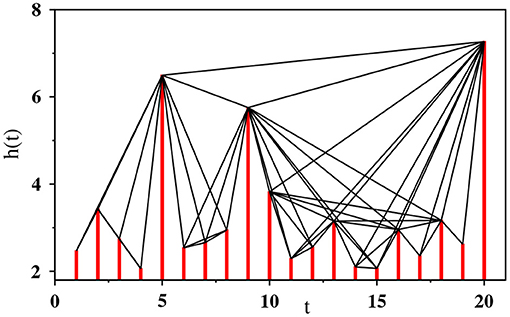
Figure 1. Visibility graph representation of a synthetic time series with 20 data values drawn randomly from an exponential distribution, where t_i = i is the time t corresponding to the i-th data. Each vertical bar representing the height variable h is considered as a node and if the top of one bar is visible from the top of the another then a link is placed between the corresponding pair of nodes.

If there exists visibility, the slope s_ij of the line between the nodes i and j must be the maximum of the slopes s_ik for all i < k < j. Therefore, a link is placed between two nodes i and j in the visibility graph if and only if for all t_i < t_k < t_j the following criterion is satisfied:

$\begin{array}{ll}{h}_k<h_i+(h_j-h_i)\frac{t_k-t_i}{t_j-t_i}.& (3)\end{array}$

Clearly, every node is visible at least from its left and right nearest neighbors and thus one obtains a completely connected network.

The “divide & conquer” algorithm [29] has been used to efficiently transform a time series into its corresponding visibility graph. This algorithm takes advantage of the fact that the node with the maximum height divides the time series into two segments in the sense that the nodes situated at one side of the maximum are not visible from the another side. Therefore, it is not required to check the visibility between the two sides of each separated segments. In each step, the visibility of the node with the maximum height to the other nodes at its right and left sides is determined. Each new segment is then treated independently and the same procedure is repeated until every segment contains one single node. The CPU time taken by the algorithm scales with the size N of a time series as NlogN.

2.2. Description of the Seismic Catalog

In a seismic catalog, an event is described by the location of the hypocenter, the time of occurrence, and the magnitude (M). We select several representative regions from Japan and California since these two areas are well-known for intense seismic activity and dense monitoring networks. The catalog data we analyze here are provided by the Japanese Meteorological Agency¹, the Hot Spring Research Institute [30], the Southern California Earthquake Center [31], the World Tremor Database [32], and Slow Earthquake Database [33], respectively.

A selected region is described by the minimum and the maximum of the latitude (θ) and longitude (ϕ) coordinates, i.e., the values of (θ_min, ϕ_min) and (θ_max, ϕ_max). We consider only the crustal events within the depth of 50 km. For the regular and the swarm earthquakes, we also indicate the magnitude of completeness M_c i.e., the lowest magnitude above which the GR law holds. Above this completeness magnitude, missing events in a catalog should be rare and therefore, effects of missing events should be minimized. We determined these values using the Zmap software tool [34]. For tremors, we consider all detected events recorded in the two previously mentioned database [35, 36]. The total number of events in a catalog is denoted by N_t. The detailed specifications of these catalogs data are given in Table 1.

TABLE 1

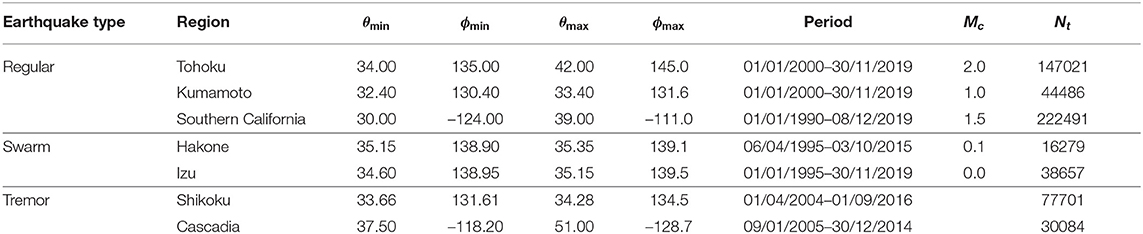
Table 1. The summary of the catalog data analyzed for investigating the correlations between the earthquake events.

2.3. Remarks on Regional Specifics

For time series of regular earthquakes, we analyzed three active seismic regions located in different tectonic settings: subduction, compression, and active faulting. The region named Tohoku corresponds to an offshore area of the Japan Trench subduction zone where the 2011 earthquake of moment magnitude M_w9.0 and its aftershocks were recorded. Time series before and after the M_w9.0 event are referred here as Tohoku₁ and Tohoku₂, respectively. The Southern California region is located in a complex compressional tectonic setting dominated by the southern part of the San Andreas Fault system, but also includes earthquakes generated by the slow uplifting of the Sierra Nevada Mountain range, as well as volcanic and geothermal related activity. The Kumamoto region mostly includes the recent seismic activity generated by the 2016 M_w7.0 Kumamoto earthquake around the active Futagawa-Hinagu fault and the surrounding active volcanic region of Aso-Yufuin-Beppu. Thus, most earthquakes in the Kumamoto catalog are aftershocks. In the Hakone volcanic region, significant swarm activity was detected since 2001 [37]. Although many different swarm episodes were recorded, they don't exhibit any specific temporal pattern. An increase in the seismicity level was observed in 2015 due to a volcanic eruption [38]. The Izu volcanic region is characterized by magma-intrusion episodes which generate frequent swarm activity [39]. Concerning the tremor activity, we selected two areas where the largest number of detected events is available, such as Cascadia in North America and Shikoku around the Nankai Trough in Japan.

3. Analyses on Magnitude Time Series

3.1. Stretched Exponential Nature of Degree Distribution

To investigate whether the magnitude of earthquakes has any correlations, we study the degree distribution of the visibility graph constructed from the magnitude time series.

First we check if the degree distribution is power law. Typically, a power law distribution is characterized by a long tail that develops with the network size N in such a manner that the average maximum nodal degree 〈k_max(N)〉 grows as $\langle k_{\text{max}}(N)\rangle \propto N^{\alpha }$. This signifies the existence of power-law degree distribution for the infinitely large network, N → ∞. In order to do this analysis, the original time series is divided into several segments such that each segment contains exactly N number of events.

We start with our results for regular earthquakes in the Tohoku region. Since the period of Tohoku₂ is exceptionally active after the occurrence of the magnitude 9.0 earthquake, we have analyzed the data for Tohoku₁ and Tohoku₂ separately. In Figures 2A,B, the degree distribution of the visibility graph is shown on a double logarithmic scale for four values of N starting from 2¹⁰ to 2¹³, at each step N being increased by a factor of 2. For all the four values of N in both the cases (Tohoku₁ and Tohoku₂), the curves have certain amount of curvature and the tails of the degree distributions do not elongate significantly as N increases. To see this dependence more clearly, we have plotted the average maximum nodal degree 〈k_max(N)〉 against N on a semilog scale in Figure 2C. Clearly, this implies that 〈k_max(N)〉 ~ ln N, demonstrating that the degree distribution is not a power law: namely, the absence of fBm-like structure in the magnitude time series.

FIGURE 2

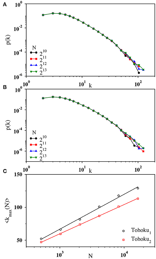
Figure 2. Log-log plot of the binned data for degree distribution p(k) associated with the magnitude time series (A) Tohoku₁ and (B) Tohoku₂ for network sizes N = 2¹⁰ (black), 2¹¹ (red), 2¹² (blue), and 2¹³ (green). (C) The variation of the average maximum nodal degree 〈k_max(N)〉 with N on a lin-log scale for Tohoku₁ (black) and Tohoku₂ (red) using N = 2⁹ to 2¹⁴. The fit (solid line) of the data points by a straight line indicating the logarithmic growth of 〈k_max(N)〉.

Specifically, the degree distribution appears to follow a stretched exponential function:

$\begin{array}{ll}p(k)=A{e}^{-{\left(\frac{k}{k_0}\right)}^{\tau }}& (4)\end{array}$

In Figure 3A, we have plotted the degree distribution p(k) of the visibility graph on a log-log scale for the whole time series of Tohoku₁ and Tohoku₂ containing 55824 and 91197 events, respectively. The logarithmically binned data for both the series fits quite well with the above functional form in the range of k between 6 to approximately 100. This is shown more explicitly in Figure 3B, where p(k) is replotted against k^τ on a semilog scale. The curves are straight in the intermediate region, indicating that the distribution follows an exponentially decaying function of k^τ. This behavior is also evident from the cumulative degree distribution shown in Figure 3B (inset).

FIGURE 3

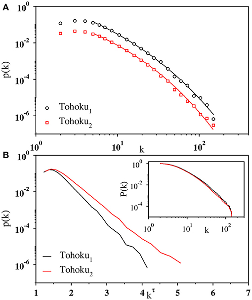
Figure 3. (A) Log-log plot of the binned data (open circles) for degree distribution p(k) of the whole magnitude time series Tohoku₁ (black) and Tohoku₂ (red). The solid lines are the fit of the corresponding data using Equation (4) whose parameters are A = 195.0 and 57.68, 1/k₀ = 210.0 and 51.03, and τ = 0.284. and 0.325, respectively. The data for Tohoku₂ has been shifted vertically for visual clarity. (B) Plot of the same data against k^τ, with k being the degree of the nodes, on a semilog scale exhibits a straight line in the intermediate regime. Inset: log-log plot of the cumulative degree distribution P(k) for the corresponding data sets.

To confirm the ubiquity of the stretched exponential nature of degree distribution, we analyze the other six earthquake catalogs. Figure 4 shows degree distributions presented similarly to those in Figure 3B for Southern California (regular), Hakone (swarms), and Shikoku (tremors). Apparently, these degree distributions are fitted with the stretched-exponential function irrespective of the region or the earthquake type. The cumulative degree distributions are also shown in Figure 4 (inset).

FIGURE 4

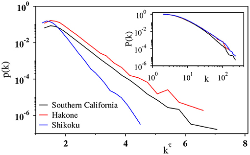
Figure 4. Plot of the degree distribution p(k) against k^τ, with k being the degree of the nodes, on a semilog scale for the time series of Southern California (black), Hakone (red), and Shikoku (blue). The τ values are 0.364, 0.364, and 0.280, respectively. The plot indicates exponential decay of all the curves. For visual clarity, a linear shift is given to the black curve [p(k) = p(k)/2]. Inset: log-log plot of the cumulative degree distribution P(k) for the corresponding data sets displaying systematic curvatures of the curves.

Furthermore, two important points should be remarked regarding the robustness of the above result. First, the stretched exponential nature does not significantly change even when the cutoff magnitude M_c is set to be lower or slightly higher than the completeness magnitude: Namely, the result is rather insensitive to some undetected smaller events. This may be because the tail of the degree distribution is controlled by events of larger magnitude, which generally have higher visibility. Second, we confirm that the shape of degree distribution is unaltered even if the time series is with respect to the event index instead of the real occurrence time. Namely, the degree distribution remains stretched exponential even if the event time t_i is replaced by an integer i in the visibility criterion, Equation (3).

3.2. Degree Distribution for Shuffled Data

Hereafter we refine the analysis and argue if there are any other correlations in the magnitude time series. To this end, we first analyze the visibility graph produced from the shuffled time series. Namely, by randomly choosing a pair of events, their respective magnitudes are swapped. This process is repeated by N_t times (the number of events in the catalog), leading to one shuffled sequence. This procedure preserves the probability density function of magnitude but destroys any potential correlations between them. Then, for a shuffled sequence, the visibility graph is constructed and the degree distribution is calculated. This process is repeated for many times and the degree distributions are averaged over these shuffled sequences. The averaged degree distribution is shown in Figure 5 (main panel). This is again fitted with the stretched exponential distribution. The same is true for the degree distribution of each shuffled sequences, and the curves are not distinguishable from the original time series (inset of Figure 5). This again validates the absence of fBm-like correlations in the original sequence.

FIGURE 5

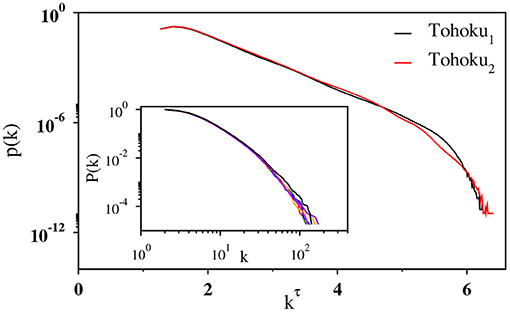
Figure 5. Main panel: Semilog plot of the degree distribution, p(k) vs. k^τ, with k being the degree of the nodes, for the shuffled series corresponding to Tohoku₁ (black) and Tohoku₂ (red). The plot is based on 10⁶ independent shuffled series. Inset: Log-log plot of the cumulative degree distribution P(k) for six individual shuffled series of Tohoku₁ (different colors are used to represent different shuffled series) along with the original one (black).

3.3. Kolmogorov-Smirnov Test

More importantly, however, the above analysis does not mean that there are no correlations in earthquake magnitude, since the averaging process may mask some subtle short-range irregular correlations. To scrutinize the statistical difference in the visibility graph structure of the original and the shuffled time series, we perform the Kolmogorov-Smirnov (KS) test. Here the null hypothesis is that two empirical degree distributions originate from the same function for the original time series and its shuffled sequence. We adopt the 0.05 significance level and reject this null hypothesis if the p-value is smaller than 0.05. In this formulation, rejecting the null hypothesis means that the degree distributions are different for two visibility graphs produced from the original time series and its shuffled one.

Specifically, the KS test statistic is computed as a distance between two empirical degree distributions produced from the original time series and its shuffled one. Then the p-value is calculated from the distance. This procedure is repeated for many shuffled sequences to yield the distribution of the p-value. They are shown in Figure 6A for Tohoku₁ (regular earthquakes) and Figure 6C for Cascadia (tremors). Apparently, the null hypothesis is rejected for both the cases. Namely, the degree distributions are not the same for the original time series and the shuffled surrogates. We also find that the null hypothesis is rejected for all the other catalogs shown in Table 1. This implies that the visibility structure in the original time series is somewhat altered if shuffled. In other words, the original time series can be discriminated among many other shuffled data.

FIGURE 6

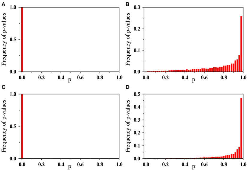
Figure 6. Normalized frequency distribution of the p-values computed from the KS test statistic between two degree distributions: (A,C) Comparison of degree distributions for the original time series and its shuffled ones. (B,D) Comparison of degree distributions for two shuffled time series obtained from a given original time series. In each panel, the data is obtained from 10⁴ shuffled series. The upper and lower panel correspond to the time series of Tohoku₁ and Cascadia, respectively.

To support the above statement from another aspect, we again perform the KS test by comparing a specific shuffled time series with many other shuffled ones. The distribution functions for the p-value are shown in Figures 6B,D. In this case, the null hypothesis is not rejected at the 0.05 significance level. Namely, shuffled time series are indistinguishable in terms of the degree distribution of their visibility graphs. This makes a quite contrast to the original time series, which is distinguishable from shuffled ones.

3.4. Analyses on Three Other Surrogates

In addition to shuffled time series investigated above, we inspect three other surrogate data. The first and the second ones are the random time series, in which the height values {h_i} are drawn randomly and independently from an exponential distribution p(h) ~ e^−λh between [2, 9]. For the first surrogate data, the time is set to be the event index: i.e., t_i = i for the i-th event. Note that λ is proportional to the b-value in the GR law as λ = 2.303b. In Figure 7, the degree distribution p(k) are shown for several values of λ. Each curve is seen to follow the stretched exponential form. Similar to the original earthquake data, 〈k_max(N)〉 grows logarithmically with N (not shown). This makes a contrast to the exponential degree distribution observed for the uniformly distributed heights [10].

FIGURE 7

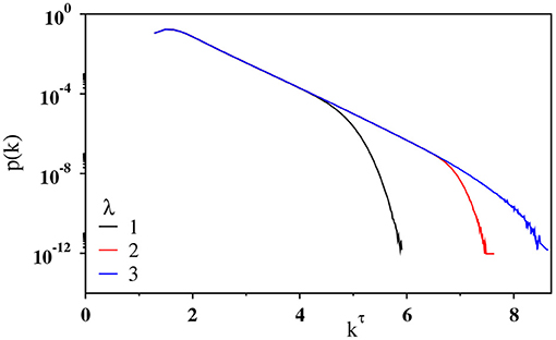
Figure 7. Plot of the degree distribution p(k) against k^τ with τ = 0.36 for the visibility graph associated with a random time series of N = 2²⁰ exponentially distributed data values on a semilog scale for λ = 1 (black), 2 (red), and 3 (blue).

The second surrogate data is the Poisson model, where events occur according to the Poisson process, and the height values are again drawn randomly from the GR law. We confirm that this surrogate data also produces the stretched exponential degree distribution. However, in the KS test that compares the surrogate data and the original magnitude series, the null hypothesis is rejected. Namely, they don't yield the same degree distribution.

The third surrogate data we wish to inspect is a time series with a short memory. Here the time series is generated by simulating a Brownian particle in one dimension subjected to a linear potential: U(x) = c|x|. Starting from x = 0 at time t = 0, the position of the particle is updated in steps of dt = 10⁻⁶ according to the following Langevin equation:

$\begin{array}{ll}x\left(t+dt\right)=\{\begin{array}{ll}x\left(t\right)-cdt+\sqrt{dt}\xi \hfill & \text{for} x⩾0,\hfill \\ x\left(t\right)+cdt+\sqrt{dt}\xi \hfill & \text{for }x<0,\hfill \end{array}& (5)\end{array}$

where ξ is a Gaussian white noise with zero mean and unit variance. The height distribution for x(t) follows the Boltzmann-Gibbs distribution at equilibrium. Since the potential is linear, the distribution function is exponential, as confirmed in Figure 8A. We construct the visibility graph using the time series of x(t) and compute the degree distribution. As shown in Figure 8B with four different system sizes N, the degree distribution is observed to follow a power law. Additionally, we confirm that 〈k_max(N)〉 grows as a power-law with N: i.e., $\langle k_{\text{max}}(N)\rangle ~N^{0.486(5)}$ (not shown). This signifies that a systematic single step memory in the time series leads to a scale-free network.

FIGURE 8

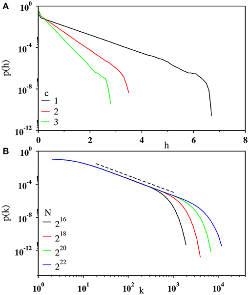
Figure 8. (A) Plot of the height distribution p(h) of the time series generated from the Brownian motion of a particle confined in a linear potential U(x) = c|x| on a semilog scale for c = 1 (black), 2 (red), and 3 (green). The slopes of the curves are found to be 1.98(3), 3.95 (3), and 5.98(3), respectively. (B) Log-log plot of the degree distribution p(k) of the visibility graph corresponding to the time series of c = 1 for N = 2¹⁶ (black), 2¹⁸ (red), 2²⁰ (green), and 2²² (blue). The dotted line is the guide to the eye with slope 2.01. The results are based on the averages of at least 10³ independent trajectories.

All the findings above lead us to conclude that the time series of earthquake magnitude are not statistically identical to uncorrelated time series, although no apparent systematic memories exist, either long-ranged (fBm-like) or short-ranged.

4. Correlation Between the Inter-Event Times

4.1. Power-Law Nature of Degree Distribution for Tohoku Data

To characterize the temporal correlations between seismic events and to understand whether they are dependent on specific details of the seismic activity, we focus on studying the inter-event time (IET) series of earthquakes. Here the IET series is obtained from an earthquake catalog by calculating time intervals between two consecutive events and labeling them with the event index i. Namely, the IET series is represented as (i, h_i), where h_i = t_i+1 − t_i, and t_i is the real occurrence time of the i-th event in a catalog. Here the threshold is set as the completeness magnitude M_c (listed in Table 1).

Figure 9A shows the cumulative degree distribution P(k) for the IET series of Tohoku₁ and Tohoku₂. This is the probability of finding a node with degree at least k in the visibility graph. For both the cases, the degree distribution is found to be heavy-tailed distribution and the tail extending more than one decade can be described by an approximate power law. We estimate the exponent: γ = 2.34(5) for the Tohoku₁ and γ = 2.60(8) for the Tohoku₂. The average maximum nodal degree also varies as a power law: $\langle k_{\text{max}}(N)\rangle ~k^{\alpha }$, where α = 0.77(3) and 0.53(4) for the Tohoku₁ and Tohoku₂, respectively (not shown here). This behavior supports the power law nature of the degree distribution. Thus, the visibility graphs constructed from the IET series exhibit typical signatures of a scale-free network, indicating the existence of fBm-like correlations in the time series.

FIGURE 9

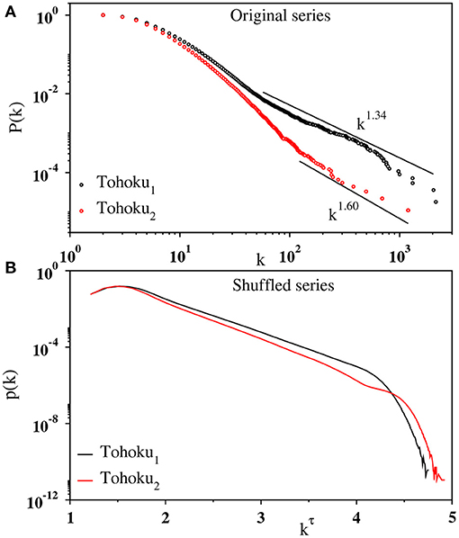
Figure 9. (A) Log-log plot of the cumulative degree distribution P(k) for the IET series of Tohoku₁ (black) and Tohoku₂ (red). The slope of the curve in the fitted region (solid line) has been estimated as 1.34(5) and 1.60(8), respectively. (B) The degree distribution p(k) shown as a function of k^τ with k being the degree of the nodes for shuffled sequences of the corresponding data on a semi-log scale. Here the exponent τ is estimated as 0.30 and 0.28, respectively.

To validate the presence of correlation in a contrasting manner, we analyze the shuffled sequences of the IET data and find that the degree distribution p(k) is fitted with the stretched exponential function given in Equation (4). In Figure 9B, the degree distributions p(k) are plotted with k^τ for the shuffled IET series of Tohoku₁ and Tohoku₂. The straight line here confirms the stretched exponential form of the degree distribution. In addition, we find that 〈k_max(N)〉 ~ ln N (not shown). Evidently, the shuffled data produces the properties of a random time series and therefore provides evidence on the existence of correlation in the original time series.

4.2. Power-Law Nature of Degree Distribution: Other Regions

The same analyses are carried out for regular earthquakes in different regions, as well as for swarms and tremors. The results are shown in Figure 10. In Figures 10A–C, the cumulative degree distribution is plotted for regular earthquakes, swarms, and tremors. For every case, a heavy-tailed distribution has been observed. While for regular earthquakes and tremors a power law regime extending more than one decade is quite apparent, the data for swarms shows more complex behavior. However, an approximate power law variation can fit the data in the intermediate region. For each case, the data points in the most linear regime (estimated by eyes) starting from a moderate value of k to a value at the tail part upto which they do not fall-off due to the limitations by finite size are fitted to the best straight line. From the slope of the straight line, we estimate the power-law exponent γ as 1.73(8), 2.64(5), 1.81(9), 1.79(9), 2.51 (5), and 2.13(5) for Kumamoto (regular), Southern California (regular), Hakone (swarm), Izu (swarm), Cascadia (tremor), and Shikoku (tremor), respectively. In addition, the power law dependence of the average largest degree 〈k_max(N)〉 with N has been observed for every set of data (not shown), supporting the power law nature of the degree distribution.

FIGURE 10

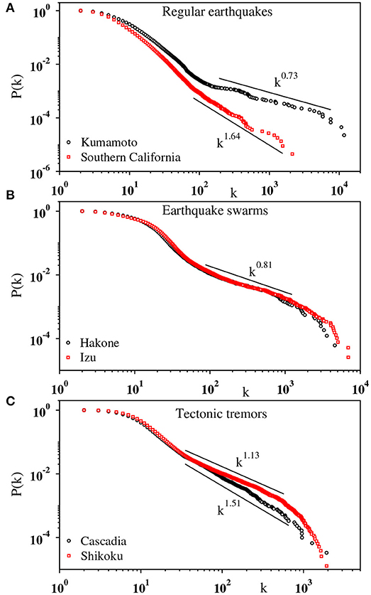
Figure 10. Log-log plot of the cumulative degree distribution P(k) for the IET series of different types of earthquakes: (A) regular earthquakes in Kumamoto (black) and Southern California (red); (B) swarms in Hakone (black) and Izu (red); (C) tremors in Cascadia (black) and Shikoku (red). The slopes in the fitted region (solid line) are 0.73(8), 1.64(5), 0.81(9), 0.79(9), 1.51(5), and 1.13(5), respectively.

The tail part of the degree distribution is characterized by the exponent γ, which seems to depend on the seismic activity of the specific region: (i) Earthquake swarms (Izu and Hakone) have a common value, γ ≃ 1.8. (ii) Regular earthquakes may also have a common value, γ ≃ 2.6 (Tohoku₂ and Southern California), while it is somewhat smaller (2.3) before the Tohoku M_w9.0 earthquake (Tohoku₁). (iii) Kumamoto is exceptional with γ ≃ 1.7. This value is rather close to swarms, although the data mainly consist of aftershocks of 2016 Kumamoto earthquake. There may be two reasons for this discrepancy. First, the data is not a usual mainshock-aftershocks sequence, but rather a foreshocks-mainshock-aftershocks sequence. Alternatively, we may interpret it as two mainshocks (M_w6.2 and 7.0) that occurred within only 30 h. In any case, it is rather anomalous seismic activity. The second potential reason is an active volcano (Mt. Aso) located in the proximity of the main fault. The M_w7.0 mainshock triggered many earthquakes in the volcanic area, including an M_w5.9 event and its own aftershocks. Thus, the overall seismic activity is influenced by the nearby volcanic field and this may explain the resemblance to swarms.

If we suppose the relation between the fractional Brownian motion and the power-law degree distribution, i.e., Equation (2), the exponent for the power spectrum β can be determined. For example, swarms have β ≃ 2.2 and H ≃ 0.6. They are close to those for standard Brownian motion (β = 2 and H = 0.5) but yet slightly larger, corresponding to superdiffusion. Regular earthquakes (γ ≃ 2.6) have β = 1.4 and H = 0.2, corresponding to subdiffusion. Extraction of these exponents from actual seismic data is difficult using other standard methods such as autocorrelation functions due to the strong non-stationary nature of the seismic record. In this sense, these exponents might not be considered as that for fBM itself, but should represent some counterpart in seismic activities.

Shuffled time series again yield visibility graphs with their degree distributions of stretched-exponential form, resembling the properties of a random time series. Therefore, we confirm that the original IET series possess fBm-like correlations irrespective of the earthquake types: regular, swarms, and tremors. This result does not contradict the previous studies on regular earthquakes obtained using some different methods [40, 41]. Here we have confirmed the correlation using complex network based approach, and more importantly, found correlations in tremors and swarms.

Lastly, we wish to add a remark on catalogs on tremors. Since a single event is not as distinct as regular earthquakes, there may be some errors in the IET of tremors. To check the effect of such errors in IET, we add a certain amount of noise to the IET data of tremors and construct the visibility graph from these noisy data. We find that the degree distribution is indeed robust to the noise: it retains the power-law nature against the small noise in IET.

5. Detailed Structure of Visibility Graph

The detailed characterization of the topology of the network has served to identify several non-trivial features exhibited by diverse types of real-world systems including the basic principles that played role in the network formation [1, 3, 4]. In order to extract more properties hidden in the seismic records, the following graph-theoretical quantities have been analyzed after obtaining the visibility graph using “divide & conquer” algorithm.

Since our visibility graph is connected and undirected, there always exists at least one path between any arbitrary pair of nodes i and j through the links of intermediate nodes. The path with the minimal links traversed is called the shortest path length d_ij, and the average shortest path length is defined as,

$\begin{array}{ll}l=\frac{1}{N(N-1)}{\displaystyle \sum _{\begin{array}{c}i,j\\ i\ne j\end{array}}}{d}_{ij}.& (6)\end{array}$

In Figures 11A,B, we show the variation of l(N) with N on a semilog scale for both the magnitude and IET series, respectively. The best fit of the data by a straight line indicates its logarithmic scaling and hence, the network is small-world. Although the data for IET series of Shikoku has some curvature, the linear behavior is quite apparent for large values of N. For IET series of swarms, l(N) grows more slower than ln N.

FIGURE 11

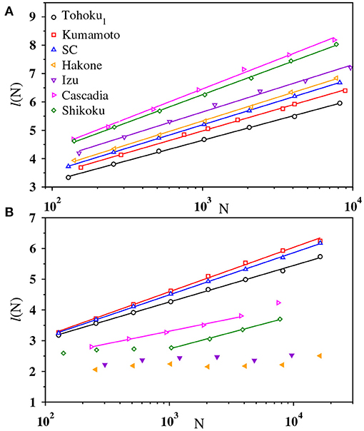
Figure 11. The plots exhibit small-world behavior of the visibility graph for (A) magnitude and (B) IET time series of Tohoku₁ (black), Kumamoto (red), Southern California (blue), Hakone (solid orange), Izu (solid violet), Cascadia (magenta), and Shikoku (green). For visual clarity data of l(N) have been shifted vertically. Multiplicative factors in the upper panel are 1, 1.05, 1.10, 1.15, 1.20, 1.25, and 1.30, respectively. In the lower panel [the labels are same as in (A)] data for swarms have been shifted as y = y/1.5.

Another important quantity associated with the network is the clustering coefficient which measures the three point correlation among the neighbors. Specifically, the clustering coefficient C_i of node i measures the probability that the two neighbors of i are connected. If there exists E_i links among the k_i neighbors of node i then, C_i = 2E_i/k_i(k_i − 1). In the case of k_i < 2, C_i = 0. The global clustering coefficient is expressed as,

$\begin{array}{ll}C=\langle C_i\rangle =\frac{1}{N}{\displaystyle \sum _{i=1}^N}\frac{2E_i}{k_i(k_i-1)}.& (7)\end{array}$

By varying N from 2⁹ to 2¹⁶ we have observed that C is almost independent of N (values differ only at 4-th decimal place) for both magnitude and IET time series of different types of earthquakes. Further, the clustering coefficient 〈C(k)〉 for the nodes with degree k has been found to decay as 〈C(k)〉 ~ k^−ν with ν ≈ 1, as shown in Figure 12. This is the universal feature of a hierarchical network observed in many real-world networks [42]. The clustering coefficient C assumes its highest value for the IET series of tremors.

FIGURE 12

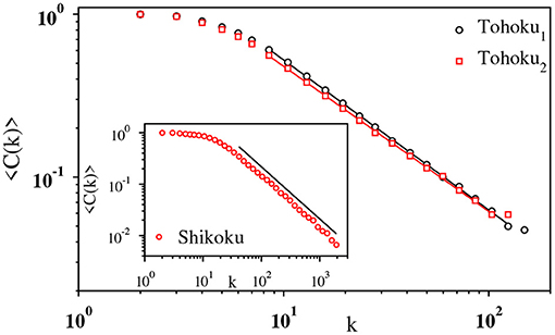
Figure 12. The hierarchical nature of the visibility graph. The clustering coefficient 〈C(k)〉 has been plotted with k on a log-log scale for the Tohoku₁ (black) and Tohoku₂ (red) magnitude time series (main panel), and for the IET series of Shikoku (inset). The slopes of the fitted lines have been measured as 0.92(3), 0.89(3), and 1.01(2), respectively.

We have also calculated the Pearson correlation coefficient r to investigate whether a high degree node tends to be linked with a high degree node (assortative mixing, r > 0) or a low degree node (disassortative mixing, r < 0). We have calculated r using the following formula [43],

$\begin{array}{ll}r=\frac{L^{-1}{\displaystyle {\sum }_i}{k}_{1i}{k}_{2i}-{\left[L^{-1}{\displaystyle {\sum }_i}\frac{1}{2}(k_{1i}+k_{2i})\right]}^2}{L^{-1}{\displaystyle {\sum }_i}\frac{1}{2}({k_{1i}}^2+{k_{2i}}^2)-{\left[L^{-1}{\displaystyle {\sum }_i}\frac{1}{2}(k_{1i}+k_{2i})\right]}^2},& (8)\end{array}$

where, k_1i and k_2i are the degrees of nodes at the ends of link i with i = 1, 2, ⋯ , L. We found that for all earthquake types, the magnitude series shows assortative nature (last column of Table 2). In contrast, in case of IET series we obtain a value of r ≈ 0 for the regular earthquakes and for swarms and tremors r < 0 (last column of Table 3). Moreover, the graph associated with the IET series of swarms has been found to be more disassortative than that of tremors. This means that for swarms the high degree nodes show more preference toward linking with the low degree nodes. This indicates that the smaller heights are abundant in both the time series, however, there are a few very large heights (i.e., long quiescence periods) in the swarms series which are even larger than the largest height in the tremor series. Therefore, swarms are more intermittent than tremors.

TABLE 2

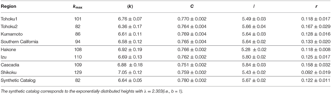
Table 2. Average values of the maximum degree k_max, average degree 〈k〉, clustering coefficient C, shortest path length l, and Pearson correlation coefficient r for the visibility graph of the magnitude time series with N = 2¹².

TABLE 3

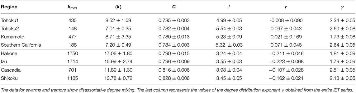
Table 3. Average values of the maximum degree k_max, average degree 〈k〉, clustering coefficient C, shortest path length l, and Pearson correlation coefficient r for the visibility graph of the inter-event time series with N = 2¹².

For a detailed comparison of the characteristic differences among the three different types of earthquakes, the above quantities have been calculated for a fixed value of N = 2¹² and the obtained values are listed in Tables 2, 3 for the magnitude and the IET series, respectively. Clearly, they can be distinguished by the values of different graph-theoretical quantities obtained from their individual IET series.

6. Discussion

Finding and characterizing any correlations in the time series of earthquake magnitude is a subject of great importance as it may be useful in forecasting major earthquakes. However, to date, existence of correlations is somewhat controversial and has not been settled [40, 44–46]. For instance, it was reported that regular earthquakes occurring close in space and time are correlated in their magnitudes [44]. A counterargument was given in [45] that these were pseudo correlations due to the magnitude incompleteness and the modified Omori law. To shed new light to this long-standing problem, we have made use of the complex network theory and analyzed the visibility graph to extract correlations in magnitude time series.

The previous studies [47, 48] in this context involve regular earthquakes only. Here we extend the analysis to two other types of earthquakes [49] to consider this problem in a more general perspective. By using the method of visibility graph, we have analyzed seismic time series in seven seismogenic zones including the regular earthquakes in Southern California in common with [48] but for more extended time period. The degree distribution appears to be fitted with a stretched exponential function for all the types of earthquakes analyzed here.

Visibility graphs are also constructed from shuffled catalogs (Figure 5) or synthetic data drawn randomly from the GR law (Figure 7). On average, the degree distribution appears to be fitted with the stretched exponential function. However, the Kolmogorov-Smirnov test rejects the null hypothesis that these degree distributions are identical. Namely, the degree distributions for these surrogate data are indeed distinguishable from that of the original data. This means that the original series have some special characters that are lost in their surrogates: shuffled or synthetic catalogs.

Since the criterion for the visibility graph involves both magnitude and IET, one might argue that the difference in the degree distribution detected by the KS test is a mere by-product resulting from the correlation in IET. To exclude this possibility, we also perform the KS test by constructing the visibility graph using the event index i instead of the occurrence time t_i. We find that the null hypothesis is again rejected. Namely, the magnitude series (i, M_i) leads to slightly different degree distributions if they are shuffled, although the difference is detectable only by the KS test. Thus, the memory should exist in magnitudes alone.

The memoryless nature of earthquake magnitudes is a basic assumption in the epidemic-type aftershock sequences (ETAS) model, which is the most successful statistical model for earthquake time series [50]. The results given here implies that the memoryless assumption in earthquake magnitude is rather approximate. Thus, if one wishes to improve statistical models for earthquake occurrence, the correlation in magnitude should be taken more seriously. To this end, the correlation found here should be defined and quantified more clearly.

The degree distributions of stretched exponential form appear to contradict some previous studies [47, 48], in which the power law tails are concluded for the magnitudes of regular earthquakes. In view of Equation (1), this may imply a fBm-like correlation in the magnitude time series. Interestingly, however, they also analyzed randomly shuffled sequences of magnitudes and did not find any significant difference in the degree distributions. This rather contradicts the existence of a fBm-like correlation. Additionally, the degree distribution obtained in [47] spans approximately one decade only, and the tails are noisy. Thus, one needs to be careful to draw a conclusion based on these data alone. In [48], the tails of the degree distributions are less noisy, but they appear to fall off from a power law at their tails. Thus, their degree distributions might be fitted with a stretched exponential function. However, the degree distribution produced from Mexican catalog appears to develop a tail that is still different from stretched exponential. We noticed that the magnitude data in the Mexican catalog do not always obey the GR law, and this may be the reason for the deviation from the stretched exponential function. However, the Mexican data require more careful and dedicated analyses to draw any decisive conclusions on specific type of magnitude correlation.

We apply the visibility-graph analysis for the characterization of the inter-event times (IET) between consecutive earthquakes. Contrary to the magnitude time series, we find an evidence of fBm-like correlations between the inter-event times. The network associated with the IET series has a scale-free nature with the exponents γ, which depends on the essential characteristics of seismic activity. In the context of the f^−β noise, the exponent γ is directly related to β. These exponents may work as a generalized and unified quantification of the intermittent nature of seismic time series. For instance, we find that the IET series for swarms are similar to superdiffusive Brownian motion, whereas those for regular earthquakes correspond subdiffusion. However, the interpretation of superdiffusive or subdiffusive nature in the IET series is yet unclear from the mechanical point of view, and should be pursued in the subsequent studies.

We have also analyzed the whole set of data using the horizontal visibility graph algorithm. For both magnitude and IET series, however, the degree distribution results in an exponential distribution and no appreciable change has been observed between these different data sets, making it harder to draw any conclusive remarks on the distinction of different time series.

7. Conclusion

In conclusion, we have investigated the correlations in the time series of magnitudes and of inter-event times (IETs) for three different categories of earthquakes in seven seismogenic zones in the world. By applying the methods of visibility graph, we show that the IET series possess correlations similar to fractional Brownian motion, and that the three categories of earthquakes have different exponents. While such an apparent correlation is absent in the magnitude series, the Kolmogorov-Smirnov test on the degree distribution reveals that the earthquake magnitudes are not statistically equivalent to an uncorrelated (random or shuffled) time series. This challenges a current popular belief that magnitude time series are random. Since current major statistical models for earthquake rate are based on this belief, these results provide us with useful constraints in developing better statistical models.

Different temporal behaviors of three categories of earthquakes are also reflected in various graph-theoretical quantities. As found from the analysis of the assortativity coefficient, the swarms are more intermittent than tremors. More graph-theoretical techniques including horizontal visibility graph [51], multiplex visibility graph [52], and recurrence networks [11] would give new criteria for categorizing or unifying different seismic activities. A novel approach for forecasting time series based on visibility graph [53] might find potential application for earthquakes. Our study therefore shows with affirmation that the visibility graph algorithm has the potentiality to capture the non-trivial complexity inherent in a time series which is non-linear and non-stationary in nature.

One can also consider more elaborated methods for the graph construction [54]. For instance, the visibility graph constructed here is undirected and unweighted. Time directionality and weighted links based on the inter-event distances would be interesting subjects. Additionally, since the spatial information of the seismic events has been disregarded here, the extension of the visibility graph method to space-time may be a promising attempt.

Together with the present results, such graph-theoretical approaches would bring benefits to statistical modeling of various types of seismic activities that cannot be reproduced by the well-established ETAS model for regular earthquakes.

Data Availability Statement

The raw data supporting the conclusions of this article will be made available by the authors, without undue reservation.

Author Contributions

SK and TH conceived and designed the study and drafted the manuscript. SK performed computer simulations and carried out the data analysis. AO and YY prepared the earthquake catalogs. All authors took part in discussing the results, reading, and approving the final version of the paper.

Funding

This study was supported by Japan Society for the Promotion of Science (JSPS) Grants-in-Aid for Scientific Research (KAKENHI) Grants Nos. JP16H06478 and 19H01811. Additional support from the MEXT under Exploratory Challenge on Post-K computer (Frontiers of Basic Science: Challenging the Limits) and the Earthquake and Volcano Hazards Observation and Research Program is also gratefully acknowledged.

Conflict of Interest

The authors declare that the research was conducted in the absence of any commercial or financial relationships that could be construed as a potential conflict of interest.

Footnotes

1. ^ftp://ftp.eri.u-tokyo.ac.jp/pub/data/jma/mirror/JMA_HYP/

References

1. Albert R, Barabási AL. Statistical mechanics of complex networks. Rev Mod Phys. (2002) 74:47–97. doi: 10.1103/RevModPhys.74.47

CrossRef Full Text | Google Scholar

2. Newman MEJ. The structure and function of complex networks. SIAM Rev. (2003) 45:167–256. doi: 10.1137/S003614450342480

CrossRef Full Text | Google Scholar

3. Newman M, Barabási AL, Watts DJ. The Structure and Dynamics of Networks. Princeton, NJ: Princeton University Press (2006).

Google Scholar

4. Boccaletti S, Latora V, Moreno Y, Chavez M, Hwang DU. Complex networks: structure and dynamics. Phys Rep. (2006) 424:175–308. doi: 10.1016/j.physrep.2005.10.009

CrossRef Full Text | Google Scholar

5. Abe S, Suzuki N. Scale-free network of earthquakes. Euro Phys Lett. (2004) 65:581–6. doi: 10.1209/epl/i2003-10108-1

PubMed Abstract | CrossRef Full Text | Google Scholar

6. Baiesi M, Paczuski M. Scale-free networks of earthquakes and aftershocks. Phys Rev E. (2004) 69:066106. doi: 10.1103/PhysRevE.69.066106

PubMed Abstract | CrossRef Full Text | Google Scholar

7. Hope S, Kundu S, Roy C, Manna SS, Hansen A. Network topology of the desert rose. Front Phys. (2015) 3:72. doi: 10.3389/fphy.2015.00072

CrossRef Full Text | Google Scholar

8. Zhang J, Small M. Complex network from pseudoperiodic time series: topology versus dynamics. Phys Rev Lett. (2006) 96:238701. doi: 10.1103/PhysRevLett.96.238701

PubMed Abstract | CrossRef Full Text | Google Scholar

9. Yang Y, Yang H. Complex network-based time series analysis. Phys A. (2008) 387:1381–6. doi: 10.1016/j.physa.2007.10.055

CrossRef Full Text | Google Scholar

10. Lacasa L, Luque B, Ballesteros F, Luque J, Nuño JC. From time series to complex networks: the visibility graph. Proc Natl Acad Sci USA. (2008) 105:4972–5. doi: 10.1073/pnas.0709247105

PubMed Abstract | CrossRef Full Text | Google Scholar

11. Donner RV, Zou Y, Donges JF, Marwan N, Kurths J. Recurrence networks—a novel paradigm for nonlinear time series analysis. New J Phys. (2010) 12:033025. doi: 10.1088/1367-2630/12/3/033025

CrossRef Full Text | Google Scholar

12. Gao ZK, Small M, Kurths J. Complex network analysis of time series. EPL. (2016) 116:50001. doi: 10.1209/0295-5075/116/50001

CrossRef Full Text | Google Scholar

13. Zou Y, Donner RV, Marwan N, Donges JF, Kurths J. Complex network approaches to nonlinear time series analysis. Phys Rep. (2019) 787:1–97. doi: 10.1016/j.physrep.2018.10.005

CrossRef Full Text | Google Scholar

14. Lacasa L, Toral R. Description of stochastic and chaotic series using visibility graphs. Phys Rev E. (2010) 82:036120. doi: 10.1103/PhysRevE.82.036120

PubMed Abstract | CrossRef Full Text | Google Scholar

15. Donges JF, Donner RV, Kurths J. Testing time series irreversibility using complex network methods. EPL. (2013) 102:10004. doi: 10.1209/0295-5075/102/10004

CrossRef Full Text | Google Scholar

16. Lacasa L, Luque B, Luque J, Nuño JC. The visibility graph: a new method for estimating the Hurst exponent of fractional Brownian motion. EPL. (2009) 86:30001. doi: 10.1209/0295-5075/86/30001

CrossRef Full Text | Google Scholar

17. Yang Y, Wang J, Yang H, Mang J. Visibility graph approach to exchange rate series. Phys A. (2009) 388:4431–7. doi: 10.1016/j.physa.2009.07.016

CrossRef Full Text | Google Scholar

18. Shao ZG. Network analysis of human heartbeat dynamics. Appl Phys Lett. (2010) 96:073703. doi: 10.1063/1.3308505

CrossRef Full Text | Google Scholar

19. Ahmadlou M, Adeli H, Adeli A. New diagnostic EEG markers of the Alzheimer's disease using visibility graph. J Neural Transm. (2010) 117:1099. doi: 10.1007/s00702-010-0450-3

PubMed Abstract | CrossRef Full Text | Google Scholar

20. Iacovacci J, Lacasa L. Visibility graphs for image processing. IEEE Trans Pattern Anal Mach Intell. (2020) 42:974–87. doi: 10.1109/TPAMI.2019.2891742

CrossRef Full Text | Google Scholar

21. Elsner JB, Jagger TH, Fogarty EA. Visibility network of United States hurricanes. Geophys Res Lett. (2009) 36:L16702. doi: 10.1029/2009GL039129

CrossRef Full Text | Google Scholar

22. Donner RV, Donges JF. Visibility graph analysis of geophysical time series: potentials and possible pitfalls. Acta Geophys. (2012) 60:589–623.

Google Scholar

23. Gutenberg B, Richter CF. Frequency of earthquakes in California. Bull Seism Soc Am. (1944) 34:185–8. doi: 10.2478/s11600-012-0032-x

CrossRef Full Text | Google Scholar

24. Hatano T, Narteau C, Shebalin P. Common dependence on stress for the statistics of granular avalanches and earthquakes. Sci Rep. (2015) 5:12280. doi: 10.1038/srep12280

PubMed Abstract | CrossRef Full Text | Google Scholar

25. Omori F. On afer-shocks of earthquakes. J Coll Sci Imp Univ Tokyo. (1894) 7:111.

Google Scholar

26. Utsu T, Ogata Y, Matsu'ura SR. The centenary of the omori formula for a decay law of aftershock activity. J Phys Earth. (1995) 43:1–33. doi: 10.4294/jpe1952.43.1

CrossRef Full Text | Google Scholar

27. Hill DP. A model for earthquake swarms. J Geophys Res. (1977) 82:1347–52. doi: 10.1029/JB082i008p01347

CrossRef Full Text | Google Scholar

28. Obara K. Nonvolcanic deep tremor associated with subduction in Southwest Japan. Science. (2002) 296:1679–81. doi: 10.1126/science.1070378

PubMed Abstract | CrossRef Full Text | Google Scholar

29. Lan X, Mo H, Chen S, Liu Q, Deng Y. Fast transformation from time series to visibility graphs. Chaos. (2015) 25:083105. doi: 10.1063/1.4927835

PubMed Abstract | CrossRef Full Text | Google Scholar

30. Yukutake Y, Honda R, Harada M, Arai R, Matsubara M. A magma-hydrothermal system beneath Hakone volcano, central Japan, revealed by highly resolved velocity structures. J Geophys Res Solid Earth. (2015) 120:3293–308. doi: 10.1002/2014JB011856

CrossRef Full Text | Google Scholar

31. Southern California Earthquake Data Center. Earthquake Catalogs (2020). Avaialble online at: https://service.scedc.caltech.edu/eq-catalogs/date_mag_loc.php

Google Scholar

32. World Tremor DataBase. Welcome to the World Tremor Database (2020). Available online at: http://www-solid.eps.s.u-tokyo.ac.jp/~idehara/wtd0/Welcome.html

Google Scholar

33. Science of Slow Earthquake. Slow Earthquake Database (2020). Available online at: http://www-solid.eps.s.u-tokyo.ac.jp/~sloweq/

Google Scholar

34. Wiemer S. A software package to analyze seismicity: ZMAP. Seismol Res Lett. (2001) 72:373–82. doi: 10.1785/gssrl.72.3.373

CrossRef Full Text | Google Scholar

35. Idehara K, Yabe S, Ide S. Regional and global variations in the temporal clustering of tectonic tremor activity. Earth Planet Space. (2014) 66:66. doi: 10.1186/1880-5981-66-66

CrossRef Full Text | Google Scholar

36. Mizuno N, Ide S. Development of a modified envelope correlation method based on maximum-likelihood method and application to detecting and locating deep tectonic tremors in Western Japan. Earth Planets Space. (2019) 71:40. doi: 10.1186/s40623-019-1022-x

CrossRef Full Text | Google Scholar

37. Honda R, Ito H, Yukutake Y, Harada M, Yoshida A. Features of hypocental area of swarm earthquakes in Hakone Volcano in 1970's revealed by re-analysis using S-P data : comparison with recent activities. Bull Volcanol Soc Jpn. (2011) 56:1–17. doi: 10.18940/kazan.56.1_1

CrossRef Full Text | Google Scholar

38. Yukutake Y, Honda R, Harada M, Doke R, Saito T, Ueno T, et al. Analyzing the continuous volcanic tremors detected during the 2015 phreatic eruption of the Hakone volcano. Earth Planets Space. (2017) 69:164. doi: 10.1186/s40623-017-0751-y

CrossRef Full Text | Google Scholar

39. Hayashi Y, Morita Y. An image of a magma intrusion process inferred from precise hypocentral migrations of the earthquake swarm east of the Izu Peninsula. Geophys J Int. (2003) 153:159–74. doi: 10.1046/j.1365-246X.2003.01892.x

CrossRef Full Text | Google Scholar

40. Corral A. Dependence of earthquake recurrence times and independence of magnitudes on seismicity history. Tectonophysics. (2006) 424:177–93. doi: 10.1016/j.tecto.2006.03.035

CrossRef Full Text | Google Scholar

41. Fan J, Zhou D, Shekhtman LM, Shapira A, Hofstetter R, Marzocchi W, et al. Possible origin of memory in earthquakes: real catalogs and an epidemic-type aftershock sequence model. Phys Rev E. (2019) 99:042210. doi: 10.1103/PhysRevE.99.042210

PubMed Abstract | CrossRef Full Text | Google Scholar

42. Ravasz E, Barabási AL. Hierarchical organization in complex networks. Phys Rev E. (2003) 67:026112. doi: 10.1103/PhysRevE.67.026112

CrossRef Full Text | Google Scholar

43. Newman MEJ. Assortative mixing in networks. Phys Rev Lett. (2002) 89:208701. doi: 10.1103/PhysRevLett.89.208701

CrossRef Full Text | Google Scholar

44. Lippiello E, de Arcangelis L, Godano C. Influence of time and space correlations on earthquake magnitude. Phys Rev Lett. (2008) 100:038501. doi: 10.1103/PhysRevLett.100.038501

PubMed Abstract | CrossRef Full Text | Google Scholar

45. Davidsen J, Green A. Are earthquake magnitudes clustered? Phys Rev Lett. (2011) 106:108502. doi: 10.1103/PhysRevLett.106.108502

CrossRef Full Text | Google Scholar

46. Lippiello E, Godano C, de Arcangelis L. The earthquake magnitude is influenced by previous seismicity. Geophys Res Lett. (2012) 39:L05309. doi: 10.1029/2012GL051083

PubMed Abstract | CrossRef Full Text | Google Scholar

47. Telesca L, Lovallo M. Analysis of seismic sequences by using the method of visibility graph. EPL. (2012) 97:50002. doi: 10.1209/0295-5075/97/50002

PubMed Abstract | CrossRef Full Text | Google Scholar

48. Aguilar-San Juan B, Guzmán-Vargas L. Earthquake magnitude time series: scaling behavior of visibility networks. Eur Phys J B. (2013) 86:454. doi: 10.1140/epjb/e2013-40762-2

CrossRef Full Text | Google Scholar

49. Obara K, Kato A. Connecting slow earthquakes to huge earthquakes. Science. (2016) 353:253–7. doi: 10.1126/science.aaf1512

PubMed Abstract | CrossRef Full Text | Google Scholar

50. Ogata Y. Statistical models for earthquake occurrences and residual analysis for point processes. J Am Stat Assoc. (1988) 83:9–27. doi: 10.1080/01621459.1988.10478560

CrossRef Full Text | Google Scholar

51. Luque B, Lacasa L, Ballesteros F, Luque J. Horizontal visibility graphs: exact results for random time series. Phys Rev E. (2009) 80:046103. doi: 10.1103/PhysRevE.80.046103

PubMed Abstract | CrossRef Full Text | Google Scholar

52. Lacasa L, Nicosia V, Latora V. Network structure of multivariate time series. Sci Rep. (2015) 5:15508. doi: 10.1038/srep15508

PubMed Abstract | CrossRef Full Text | Google Scholar

53. Zhao J, Mo H, Deng Y. An efficient network method for time series forecasting based on the DC algorithm and visibility relation. IEEE Access. (2020) 8:7598–608. doi: 10.1109/ACCESS.2020.2964067

CrossRef Full Text | Google Scholar

54. Xu P, Zhang R, Deng Y. A novel visibility graph transformation of time series into weighted networks. Chaos Solitons Fract. (2018) 117:201–8. doi: 10.1016/j.chaos.2018.07.039

CrossRef Full Text | Google Scholar