3D Direct Numerical Simulation on the Emergence and Development of Aeolian Sand Ripples

1 Introduction

Aeolian sand ripples are commonly observed in the deserts of Earth and some other planets, which exhibit regular patterns with wavelengths that vary from centimeters to tens of meters and amplitudes that vary from millimeters to centimeters. Ripples’ morphological characteristics are wrinkle-like stripes perpendicular to the wind direction and almost symmetrical in the transverse direction. General sand ripples emerge rapidly in a continuous wind field and keep growing until they reach a saturated state. Its development process is always separated into two stages which are called the linear stage and the nonlinear stage. Starting from the phenomenological description developed by Anderson [1], researchers found that the linear stage is the first stage of ripple formation, in which the most unstable mode of the ripples’ amplitude grows exponentially. After the initiation of the ripple instability, nonlinear behavior such as the coarsening process takes place [9, 28, 34] and the ripple growth rate slows down. The formation of the sand ripple bedform has been considered as an important research subject in planetary geology since the last century on account of the reflection of local atmospheric conditions and granulometric property. However, due to the difficulty of direct observation, the causes of many distinct ripple properties remain as unsolved questions. Thus, a proper model on the development of ripple morphology is required.

To research sand ripples, an eligible model should be able to correctly reproduce the rule of aeolian sand movement because the emergence and development of aeolian sand ripples are currently found to have a strong relationship to the sand transport process. Commonly, sand particles are transported by the wind in three major ways: reptation (or creep), saltation, and suspension. The saltating particles are those going forward by bouncing on the bed and splashing other ejected particles. These particles’ trajectories are high enough to regain the impacting energy loss from the wind and support them to travel a long distance. According to Bagnold’s seminal work [6], the formation of sand ripples is only influenced by the characteristic saltation length. However, his theory was disproved by experimental results [33, 36], which indicate that the initial ripple wavelength is much smaller than the particle saltation length. Anderson then made a very important contribution to the research on aeolian ripples by introducing the importance of the reptation process [1]. He defined reptating particles as those sand particles motivated by the saltating process containing very low energy which can only support them to have one small hop. After one hop, a reptating particle dies immediately without inciting any new particles into the air. Anderson argued that the ripple formation mechanism was entirely attributed to the contribution of reptating particles.

According to Anderson’s assumption, many theoretical models on sand ripples’ formation have been established [9, 17, 28, 34, 37, 40]. These theoretical models describe the continuous wavy bed surface as partial differential equations, which provide convenient methods to deduce the theoretical or numerical solution of bed form morphology. For many years of development, lots of refinements and development have been implemented on this kind of continuous model, making it suitable for more and more complex situations. However, no matter how advanced it is, some arbitrary simplification remains unchanged. By omitting hopping particles’ trajectories, these models simplified the description of particle dynamics and only paid attention to the initial/final location of moving particles. Saltating particles in these models do not take part in the ripple formation directly but are treated as external energy sources just bringing energies into the mass exchange system. What is more, this kind of model involves a lack of wind field information, which makes the research on the relationship between wind velocity and ripple morphology unachievable.

These drawbacks of theoretical models make people study the direct method, which contains sufficient mechanism of particles’ motion and takes into account the applied energy from the fluid field. In recent years, direct numerical simulations with particle dynamics have been frequently used for solving complex wind-blowing sand problems. Many are inspired by the work of Anderson and Haff [4]. They introduced hydrodynamic equations into the model and tracked every particle in the computation domain. Particles’ movement and the interaction between air flow and particles are carefully treated by using properly simplified momentum equations. So far, just one direct simulation work has been carried out systematically on the research of aeolian sand ripples [12]. The discrete element method (DEM) used in this work considers all the forces applied on dynamic and static particles at every moment. Because of this feature, this work suffers a great limitation on computational resources. It simulated a very short time period which is only sufficient for the initial ripple forms’ emergence. The subsequent turning point between the linear stage and the nonlinear stage cannot be directly obtained from their results, which makes them unable to take a further look at the transition between these two stages. Meanwhile, ordinary sand ripples not only develop in a timescale of tens of minutes but also require tens of thousands of particles to form a complex three-dimensional bedform. For DEM simulation, the particle number requirement of a 3D model is hard to achieve. Therefore, the simulation domain in their work is quasi-2D, which only has the length of one particle diameter in the transverse direction. Omitting the influence from the third dimension makes results less convincing, and the model will fail to explain many important 3D properties on ripple topology.

Be aware that in this work, we introduce a numerical model which just traces moving particles in the air and gains the post-collision velocity components of particles by solving the momentum equations in connection with Coulomb’s law of friction. Particles dropped into or that escaped from the sand bed are converted to the elevation deforming of the local bedform. It greatly reduced the computational costs, making long-term simulation on ripple formation processes and 3D ripple morphology simulations achievable. Thus, using this model, we can perform better studies on the relationship between multifarious wind fields and ripples’ development.

2 Method

2.1 Particle Motion

Sand particles in this simulation have been assumed to be small spheres. Every particle in the air is tracked. Despite the wake influence of particle rolling, the equation of particle velocity components is simplified as follows:

$m_p\frac{d\mathbf{v}}{dt}={\mathbf{f}}_{fp}+m_p\mathbf{g}+{\mathbf{f}}_{cp},(1)$

where $m_p$ is the particle mass, $\mathbf{v}$ is the particle velocity, ${\mathbf{f}}_{fp}$ stands for the forces of hydrodynamical origin, $\mathbf{g}$ is the gravity acceleration, and ${\mathbf{f}}_{cp}$ is the interparticle contact force. Naturally, ${\mathbf{f}}_{cp}=0$ if one particle is not in contact with another. For those particles within a contact pair, this value is not calculated directly here. The detailed dealing procedure on this term will be described in section 2.2.

The densities of the sand particle and the carrier fluid are ${\rho }_p$ and ${\rho }_f$, respectively. As the density rate $s={\rho }_p/{\rho }_f$ is large in this work and the particle diameter is much smaller than the Kolmogorov scale, the hydrodynamical force ${\mathbf{f}}_{fp}$ here is dominated by the drag force of the fluid. For a particle with a certain diameter d, the drag force exerted on it is only influenced by the relative value between its velocity $\mathbf{v}$ and the fluid velocity $\mathbf{u}$ at its position:

${\mathbf{f}}_{fp}=\frac{\pi }{8}{\rho }_f{d}^2{C}_d\left|\mathbf{u}-\mathbf{v}\right|\left(\mathbf{u}-\mathbf{v}\right).(2)$

$C_d$ is the drag coefficient. We use the following approximation that $C_d={\left(\sqrt{C_d^{\infty }}+\sqrt{R{e}_p^c/R{e}_p}\right)}^2$ [13], where $\mathit{R}{\mathit{e}}_p=\left|\mathbf{u}-\mathbf{v}\right|d/\nu$ is the particle Reynolds number which is based on relative velocity. ν is the kinematical viscosity coefficient of the fluid. $C_d^{\infty }\approx 0.5$ is the drag coefficient of the grain in the turbulence limit ($R{e}_p\to \infty$), and $R{e}_p^c\approx 24$ is the transitional particle Reynolds number.

2.2 Midair Collision and Surface Splash Function

Particles motivated from the bed are accelerated by the fluid alone in its projecting trajectory, and then some of them bombard the sand surface and entrain other particles. Momentum transfer frequently takes place via collisions among midair particles and the particles on the sandy bed during this process.

In this work, the collision event takes place while the centroid distance between a pair of particles is smaller than the sum of their radii. During the whole collision process, ${\mathbf{f}}_{cp}$ should be calculated in no time to close (1). Since equations are solved in a dispersed manner while performing the numerical simulation, $d\mathbf{v}/dt$ in (1) becomes $\Delta \mathbf{v}/\Delta t$. For the simplest linear spring model of contacting grains, the integrating during the contacting event requires the time step $\text{Δ}t$ to satisfy the limitation $\text{Δ}t=\text{Δ}{t}_c\ll T_c\ll \pi \sqrt{m_p/k}$, in which $T_c$ is the total contact time and k is the spring stiffness [4]. Considering that k for quartz particles is very large, $T_c$ could then be a very small value. In DEM simulations, this is the most significant aspect influencing the computational cost. To avoid the influence from $T_c$, in this work, the computational time step is only controlled by $T_f$. $T_f=4s{d}^2/\left(3\nu \right)$ is the relaxation time deduced from the rearranged form of (2), that is, ${\mathbf{f}}_{fp}=m_p\left(u-v\right)/T_{f}f\left(\mathit{R}{\mathit{e}}_p\right)$. For all the situations discussed in this work, $T_f$ is much larger than $T_c$. Therefore, we define the time step as $\text{Δ}t=\text{Δ}{t}_f<T_f$ and $\text{Δ}t\gg \text{Δ}{t}_c$. By this definition, we can assume that the collision happens instantaneously in every time step.

Thus, in one iteration step, the computational process of particle movement is started by solving (2) using a Runge–Kutta method under the setting that ${\mathbf{f}}_{cp}=0$. Then, instead of solving ${\mathbf{f}}_{cp}$, the post-collision velocity is determined directly by the relative velocity between two colliding particles. Here, we omit the full calculation process and just provide the result for the post-collision velocity ${\mathbf{v}}_1^{\prime }$ on one of the particles after colliding [7]:

$\begin{array}{cc}{\mathbf{v}}_1^{\prime }=& {\mathbf{v}}_1-\frac{m_2}{m_1+m_2}\left(1+\epsilon \right)\left(\mathbf{n}\cdot {\mathbf{v}}_{12}\right)\mathbf{n}-\frac{m_2}{m_1+m_2}\frac{1-\mu }{1+q}\left[{\mathbf{v}}_{12}-\left(\mathbf{n}\cdot {\mathbf{v}}_{12}\right)\mathbf{n}\right]\\ & +\frac{1}{2}\frac{m_2}{m_1+m_2}\frac{1-\mu }{1+q}\mathbf{n}\times \left(d_1{\mathit{\omega }}_1+d_2{\mathit{\omega }}_2\right),\end{array}(3)$

where the variables with subscript 1 or 2 refer to the quantities of each particle in the collision pair and ${\mathbf{v}}_{12}={\mathbf{v}}_1-{\mathbf{v}}_2$ is the relative velocity before collision; $\mathbf{n}$ is a unit vector from one particle center pointing to the center of the other one; ε and μ are microscopic restitution coefficients for the normal and tangential components, respectively; and q is a parameter which depends on the moment of inertia $I_{\mathrm{1,2}}$ on the particle as shown below:

$q=\frac{1}{4}\frac{m_1{m}_2}{m_1+m_2}\left(\frac{d_1^2}{I_1}+\frac{d_2^2}{I_2}\right).(4)$

Since the particles are assumed to be spheres, $I_{\mathrm{1,2}}=m_{\mathrm{1,2}}{d}_{\mathrm{1,2}}^2/10$ and thus $q=5/2$.

The rotation of particles is not in the consideration of this work; then we have ${\mathit{\omega }}_{\mathrm{1,2}}=0$. (3) is reduced to the following:

${\mathbf{v}}_1^{\prime }={\mathbf{v}}_1-\alpha \left(\mathbf{n}\cdot {\mathbf{v}}_{12}\right)\mathbf{n}-\beta \left[{\mathbf{v}}_{12}-\left(\mathbf{n}\cdot {\mathbf{v}}_{12}\right)\mathbf{n}\right].(5)$

In terms of the effective restitution coefficients, we have the following:

$\alpha =\frac{1+\epsilon }{1+\eta },(6)$

$\beta =\frac{\left(2/7\right)\left(1-\mu \right)}{1+\eta }.(7)$

$\eta =m_1/m_2$ is the mess ratio of two colliding particles. The same procedure can be implemented to calculate ${\mathbf{v}}_2^{\prime }$, and there is no need to repeat it here.

If one particle in the collision pair is at rest before the collision corresponding to the scene where an impactor hits the granular bed, (5) will be solved by setting ${\mathbf{v}}_{12}={\mathbf{v}}_1$ or ${\mathbf{v}}_2=0$. The variables with subscript 2 refer to quantities of particles on the bed hereafter. After considering all possible impacting statuses, a novel splash function is introduced by Lämmel [22], from which one can estimate the properties of the particles ejected from the bed surface, such as eject velocity, eject angle, and the number of ejected bed particles.

In this splash function, ejected particles are separated into two categories at first. The first one is called rebound particles, which are former injecting particles that then bounce from the bed after the collision event. It is quantified in terms of the mean restitution coefficient $\overline{e}$ and rebound angle ${\theta }_1^{\prime }$ for a given impact angle ${\mathit{\theta }}_1$, as shown below:

$\overline{e}=\frac{\left|{\mathbf{v}}_1^{\prime }\right|}{\left|{\mathbf{v}}_1\right|}=\beta -\frac{\left({\beta }^2-{\alpha }^2\right)d_2{\mathit{\theta }}_1}{\beta \left(d_1+d_2\right)},(8)$

$P\left({\theta }_1^{\prime }|{\theta }_1\right)=\{\begin{array}{cc}\frac{\gamma \left({\theta }_1+{\theta }_1^{\prime }\right)}{{\theta }_1}\ln \left[\frac{2{\theta }_1}{\gamma {\left({\theta }_1+{\theta }_1^{\prime }\right)}^2}\right]& 0<{\theta }_1+{\theta }_1^{\prime }<2\sqrt{{\theta }_1/\gamma }\\ 0& else\end{array},(9)$

where

$\gamma =\frac{2\left(d_1+d_2\right)}{9d_2}{\left(\frac{\beta }{\alpha +\beta }\right)}^2.(10)$

Particles entrained by the impactor are called ejected particles; the kinetic energy of them can be drawn from a log-normal distribution as shown below:

$P\left(E_2^{\prime }|E_1\right)=\frac{1}{\sqrt{2\pi }\sigma E_2^{\prime }}\exp \left[-\frac{{\left(\ln E_2^{\prime }-\mu \right)}^2}{2{\sigma }^2}\right],(11)$

where $E_2^{\prime }$ is the kinetic energy of an ejected particle, $E_1=m_1{\mathbf{v}}_1^2/2$ is the energy of the impactor, and we have the following:

$\sigma =\sqrt{\lambda }\ln 2,(12)$

$\mu =\ln \left[\left(1-{\overline{e}}^2\right)E_1\right]-\lambda \ln 2,(13)$

$\lambda =2\ln \left[\frac{\left(1-{\overline{e}}^2\right)E_1}{E_{d2}}\right].(14)$

In here, $E_{d2}=m_{2}g{d}_2$ is the minimum transferred energy for a bed particle to be counted as ejecta. The number N of ejected bed grains is as follows:

$N=0.06{\left[\frac{\left(1-{\overline{e}}^2\right)E_1}{E_{d2}}\right]}^{\left(2-\ln 2\right)\ln 2}{\displaystyle {\int }_{E_{d2}}^{\infty }P\left(E_2^{\prime }|E_1\right)d{E}_2^{\prime }}.(15)$

The ejection angles of all ejected low-energy particles are set to ${90}^{\circ }$, and their initial positions are uniformly distributed near the impact point. As we are expecting a 3D model for particle entrainment upon an irregular bedform, there should be a particle trajectory component in the transverse direction (the y direction in this work). In others’ work, a random distribution in the transverse direction of the rebound angle and the ejection angle was introduced into the model [21]. This artificial treatment will not be applied here because the uneven bed surface in this model introduces the y-direction particle velocity component automatically.

In (6) and (7), the restitution coefficients ε and μ characterize the relative normal motion–caused energy losses due to the deformation and the relative tangential motion–caused energy losses due to friction, respectively. ε can be treated as a constant parameter deduced from the particles’ material property. For sand, $\epsilon =0.9$. The assumption of μ is a little more complex. To derive the simple form expression of splash functions for particle–bed collision, we consider μ as a constant. It is natural to assume that the colliding particles roll past each other, that is, $\mu =0$. For midair collision, as we know the exact velocity and location information of every collision pair, under the assumption of Coulomb friction, the tangential restitution coefficient μ can be deduced from the following [31]:

$\mu =\text{max}\left(0,1-\frac{C_f\left(1+\epsilon \right)}{2/7}\frac{v_n}{v_t}\right),(16)$

where $C_f=0.4$ [14] is the coefficient of friction, and $v_n$ and $v_t$ are relative velocities between two colliding particles in the normal and tangential directions, respectively.

2.3 Aerodynamic Entrainment

Static particles on the surface are not only motivated by impactors but also, for aeolian sand drifting, are directly entrained by the turbulence fluid. Aerodynamic entrainment plays a significant role in initiating a continuous sand flux. As the saltating process is gradually enhanced, the airborne shear stress on the sand surface (wall stress) ${\tau }_{fw}$ decreases and eventually becomes smaller than the aerodynamic entrainment threshold. In this work, the objects we studied are all under the circumstances of saturated sand flux, which means that the aerodynamic entrainment can be ignored during the simulation.

Although bed particles in saturated sand flux can not be directly lifted by air flow, their bombardment entrainment can still be slightly influenced by it. As shown before, the number and energy of ejected particles are controlled by the minimum transferred energy. This value varies while a particle on the surface receives the shear force from the wind. Figure 1 shows the free-body diagram of a particle exposed to the wind shear stress. If this particle can be barely lifted by the wind, the airborne shear force $F_s={\tau }_{fw}\pi d^2/4$, and the counter force $F_N$ from the adjacent support particle and the gravitational force $m_{p}g$ should be in the equilibrium state. In this state, ${\tau }_{fw}$ is equal to the aerodynamic entrainment threshold stress ${\tau }_{ft}$. Being aware of these, we get the following equilibrium equation:

$\frac{{\tau }_{ft}\pi d^2}{4}\text{tan}\vartheta =m_{p}g,(17)$

where ϑ stands for the angle from these two particles’ center-connecting line to the horizontal surface. Otherwise, if the equilibrium state cannot be fulfilled, an effective mass $m_{eff}$ is then introduced into the model as follows:

$\frac{{\tau }_{fw}\pi d^2}{4}\text{tan}\vartheta =\left(m_p-m_{eff}\right)g.(18)$

FIGURE 1

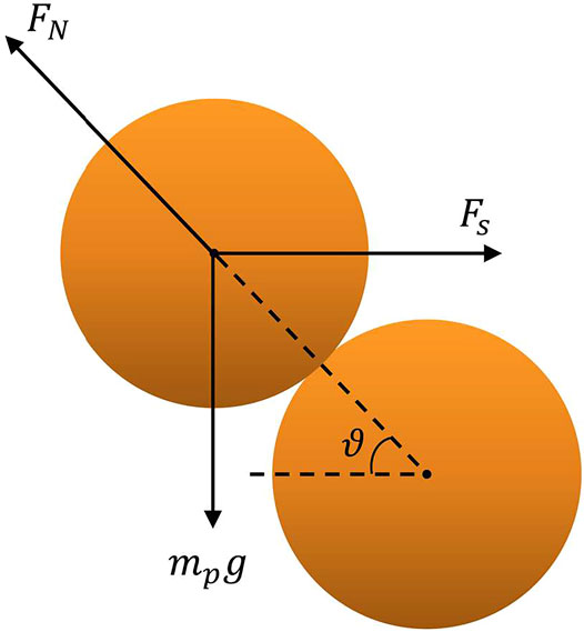
FIGURE 1. Free-body diagram of a surface particle and its adjacent neighbor exposed to the wind shear stress.

Substituting (17) into (18), we have the expression of the effective minimum transferred energy $E_{eff}$as shown below:

$\frac{E_{eff}}{E_{d2}}=\frac{m_{eff}}{m_p}=1-\frac{{\tau }_{fw}}{{\tau }_{ft}}.(19)$

In practice, during simulation, $E_{d2}$ in (14) and (15) is replaced by $E_{eff}$. The aerodynamic threshold ${\tau }_{ft}$ is deduced from Shao’s work [32].

A similar method has been used in Lämmel’s previous work [23], leading to convictive results. By employing it, reptation will be enhanced. The bed surface becomes “looser,” allowing more low-energy particles to move a tiny distance and leading to a higher frequency of midair collisions.

2.4 Hydrodynamic Governing Equations

In this study, the hydrodynamics is described using an RANS equation:

${\rho }_f\frac{\partial \overline{\mathbf{u}}}{\partial t}=-\nabla \overline{p}+{\rho }_f\left(-\nabla \cdot \overline{\mathbf{u}}\overline{\mathbf{u}}+\nabla \cdot \mathcal{T}+\frac{{\mathbf{F}}_p}{1-{\varphi }_p}\right),(20)$

where $\overline{(\cdot )}$ denotes a temporal averaged quantity. For simplicity, in what follows, we note $\mathbf{u}=\overline{\mathbf{u}}$ for the averaged fluid velocity. $\mathcal{T}$ represents the stress, which contains both viscous stress and Reynolds stress; ${\mathbf{F}}_p$ is a forcing term describing the counter force exerted by the fluid-accelerated particles; ${\varphi }_p$ is the volume fraction of particles; and $\nabla p$ is the pressure gradient. In the Eulerian field, ${\varphi }_p$ is obtained by averaging the information of Lagrange particles in grid cells. For a computational grid cell with particles in it, the following equation is applied:

${\varphi }_p=\frac{{\displaystyle {\sum }_{i=1}^{N_p}{\mathit{V}}_{p,i}}}{{\mathit{V}}_c},(21)$

${\mathbf{F}}_p=\frac{-\langle {\displaystyle {\sum }_{i=1}^{N_p}{\mathbf{f}}_{fp,i}}\rangle }{V_c},(22)$

where $N_p$ is the total particle number in this cell, $V_c$ is the cell volume, and $V_{p,i}$ is the volume of the ith particle. The symbol $\langle \cdot \rangle$ stands for ensemble averaging.

For the steady and homogeneous fluid field which we studied in this article, the inertia and horizontal stress gradients of the fluid are neglected. Regarding x as the streamwise direction and z as the vertical direction, (20) becomes the following:

$\frac{\partial {\tau }_f}{\partial z}=\frac{F_{p,x}\left(z\right)}{1-{\varphi }_p\left(z\right)},(23)$

where $F_{p,x}\left(z\right)$ and ${\varphi }_p\left(z\right)$ are the particle counter forces in fluid direction and particle volume fraction, respectively, in a thin layer at a specific altitude z. ${\varphi }_p=1$ means that the grid is full of particles. This will not happen because when the value of ${\varphi }_p$ is larger than the volume fraction of the bed particles, the hydrodynamic equations will not be calculated in the grid. Instead, the corresponding wind velocity will be set to 0 directly. A Prandtl’s mixing length model with the kinematic turbulent viscosity ${\nu }_t=l_m^2|\partial u/\partial z|$ is used to close the RANS momentum equation [35]. ${\tau }_f$ can then be expressed as follows:

${\tau }_f={\rho }_f\left(\nu +{\nu }_t\right)\frac{\partial u}{\partial z}={\rho }_f\left(\nu +l_m^2\left|\frac{\partial u}{\partial z}\right|\right)\frac{\partial u}{\partial z}.(24)$

The mixing length scale $l_m$ is provided by the following:

$l_m=\kappa z\left[1-\text{exp}\left(-\frac{1}{26}\frac{z{u}^{\text{*}}}{\nu }\right)\right],(25)$

where $\kappa =0.42$ is the von Karman’s constant and $u^{\text{*}}$ is the fractional velocity to describe the original wall shear stress of the grain-free fluid field (i.e., the fractional velocity far away from the sand bed).

Integrating (23) alone with the z direction, we obtain a drag partition equation as follows:

${\tau }_f\left(z\right)={\rho }_f{u}^{\text{*}2}-{\tau }_p\left(z\right).(26)$

${\tau }_p\left(z\right)={\displaystyle {\int }_z^{\infty }\frac{F_{p,x}\left(z^{\prime }\right)}{1-{\varphi }_p\left(z^{\prime }\right)}}d{z}^{\prime }.(27)$

${\tau }_p\left(z\right)$ is the grain-borne shear stress obtained by the following:

By combining (24)–(27), the fluid field can be calculated in a straight manner in every time step.

2.5 Topography Geometry

The bedform surface in this model is triangulated and expressed by a series of key points. We propose to establish a dynamic topography model considering bombarding particles. Thus, the key point location is variable and decided by the vicinal real-time material exchange.

To simulate the terrain, the key points in this model can move vertically and are digitalized as their elevations. We separate the bed surface into several subregions in order to estimate these elevation values. As shown in Figure 2A, the subregion is usually defined as a rectangular area (dashed line box) around every key point and plays a similar role to a sand trap. By counting all particles that drop into it or escape from it within a computational time step, the elevation change of each subregion in this time step is deduced from the following equation:

$\text{Δ}h=\frac{1}{{\varphi }_{b}A}{\displaystyle \sum }_{i=1}^{N_s}\frac{\pi d^3}{6},(28)$

where h is the elevation of a subregion, $N_s$ is the net number of the particles trapped in this subregion, and ${\varphi }_b$ is the average volume fraction of particles inside the bed. Considering that all the sand particles are assumed to be spheres, ${\varphi }_b$ is set to 0.6 in this work. A is the area of one subregion. Then, we assign the elevation of each subregion to its central key point.

FIGURE 2

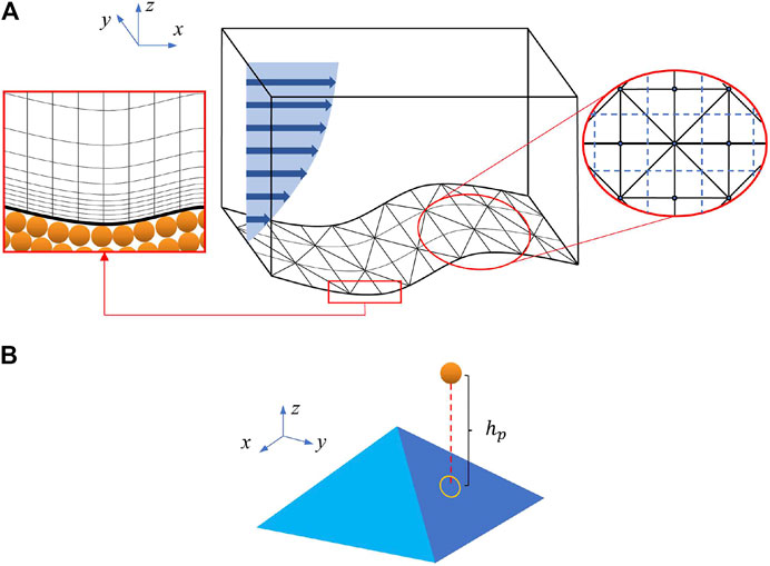
FIGURE 2. (A) Sketch of the computational domain. The left inset shows the refined grid near the bed surface. The right inset illustrates the arrangement of the surface subregion and the triangulation. (B) Sketch of a single bed surface triangulated element and the definition of $h_p$.

What should be clarified here is that the terrain generated within every calculating step is not simply a ladder-shaped surface as it is in Anderson’s simulation model [2]. Connecting all the key points of the surface generates a vivid microtopography with triangular slopes. As the sketch shown in Figure 2B indicates, the relative altitude of every particle to the surface $h_p$ is equal to the distance from the particle center to the slope surface right beneath it. The splash event occurs when $h_p$ is smaller than $0m$.

What is more, the splash function on a slope is still a matter of research and no ready-to-use model has been proposed. During the splash procedure in this model, the coordinate system of particle movement is steered toward the direction along the slope surface. In other words, for Eqs 8–15, all values of moving particles are converted to the values relative to the local bed slope. This kind of procedure seems arbitrary, but it is supported by Yin et al.’s recent work [39]. They found that for a constant impact angle relative to the bed, only the relative rebound angle shows a small decrease with the increasing bed slope angle. Other relative properties of rebound and ejected particles are nearly independent of the bed slope.

Another aspect one needs to pay attention to here is the angle of repose for every small bump and pit. We apply a natural method to regulate the behavior of particles interacting with the bed, that is, giving out the slope at every impactor’s drop point to see whether it exceeds the repose angle. If so, and if the nearest key point is a salient point, the deposited particle will roll down the slope and settle at the lowest neighbor subregion. Similarly, for erosion situations, particles that impact at a pit with a sheer slope will entrain ejectors from higher neighbor subregions. The repose angle in this work is set to ${30}^{\circ }$ for original sand particles.

2.6 Particle Size Distribution

We can calculate polydisperse situations without changing the main frame of the particle movement description. The diameter of every particle in the air is recorded. Meanwhile, a simplified procedure is added to simulate the diameter distribution of particles on the bed surface. As we know, the whole computational domain is separated into server subdomains. Every subdomain can be considered as a sand trap which contains a specific number of particles describing the local surface elevation h. Now, we separate each subdomain into several “diameter bins.” One diameter bin represents a specific particle diameter range. Particles with various diameters are sorted and dropped into corresponding bins automatically. By defining the sufficient number of diameter bins, one can describe the size distribution of bed particles. However, not all particles constituting the sand bed take part in the splash event. Only those near the surface influence the splash process. Therefore, here we introduce “affectable depth” into every subdomain standing for the depth from the surface, in which particles can be influenced by the impactor. Naturally, there is an “affectable layer” representing a layer with affectable depth covers on the sand surface. Each subdomain has its own affectable depth. Thus, for a specific subdomain, the development of surface particle size distribution has been converted to the development of the affectable depth and the diameter bins’ volume ratio within this depth.

There are three kinds of situations while dealing with the changes in the size of diameter bins and the affectable depth. Here, we use the sketch in Figure 3 to show the dealing procedures for these situations. There are 12 units in Figures 3, 4, and units in a row describe the development process within one subdomain in a specific situation. Rectangular bars in different colors represent diameter bins of different particle diameter ranges. Area of bars corresponds to the bulk volume of particles within these bins. For simplicity, we set the number of the diameter bins to 3, and they stand for surface particle sizes around $d_{\mathrm{2,1}}$, $d_{\mathrm{2,2}}$, and $d_{\mathrm{2,3}}$, respectively. The affectable depth is represented by ψ, and the magnitude of ψ is distinguished by subscripts. ${\psi }_0$ is the initial value of ψ, which is also the lowest limitation of the affectable depth. Dashed boxes point out the affectable layer. Thus, in this sketch, the area ratio of rectangular bars within the dashed box corresponds to the surface particle size distribution of a single subdomain.

FIGURE 3

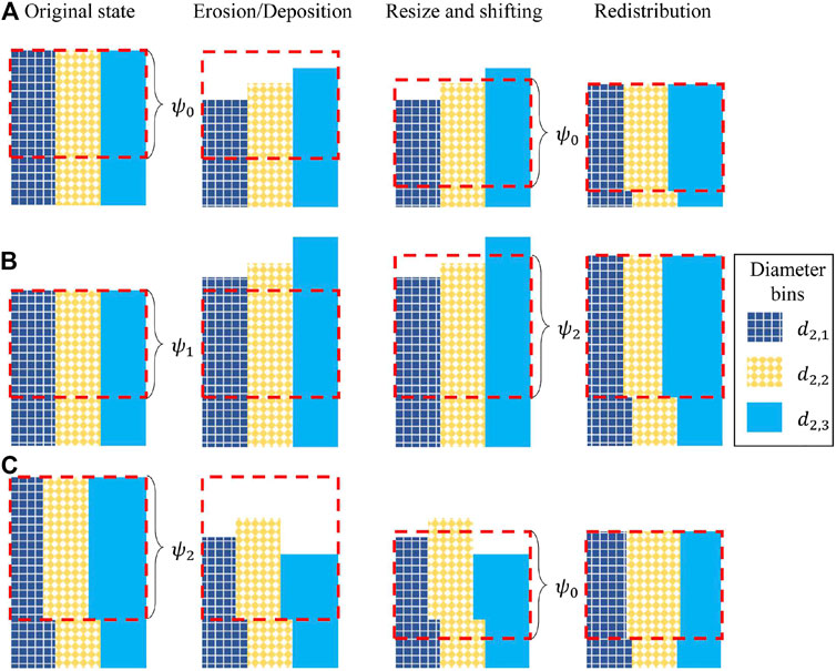
FIGURE 3. Demonstration on the surface diameter change of one subregion. The bars with different colors represent the fictitious diameter bins containing particles with a certain size. (A) The affectable layer with a smallest affectable depth ${\psi }_0$ has been eroded. The affectable layer moves downward and obtains particles from the lower bed. (B) Deposition happens at the affectable layer with an affectable depth ${\psi }_1$. The size of the affectable layer stretches. (C) Erosion happens at a stretched affectable layer. According to the eroded volume, the affectable layer will resize or move downward.

FIGURE 4

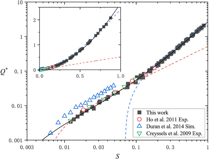
FIGURE 4. Development of nondimensional particle transport flux versus the Shields number. Inset demonstrates the same value in the linear coordinate system. The red dashed line is the linear fitting line for data points with $S<0.1$. The blue dashed line is the cubic fitting line. The black soiled line is the fitting line of (31). Hollow symbols represent data from others’ work.

For the net erosion situation with ${\psi }_0$ as the original affectable depth before the collision event, since this affectable depth cannot be smaller anymore, particles deeper inside the sand bed with initial size distribution will replenish the newly spared empty space of the affectable layer when erosion happens. This process is vividly portrayed in Figure 3A by the downward shifting of the dashed box and the following redistribution of bars inside the box. Therefore, we name these two steps as the “shifting step” and the “redistribution step.” If the situation performs as net deposition, the shifting step becomes a “resizing step.” In the resizing step, the arbitrary original affectable depth ${\psi }_1$ will increase to a larger value ${\psi }_2$ to make the space within the affectable layer sufficient to contain the extra deposited particles. This can be sketched as the resizing of the dashed box as it is shown in Figure 3B. After some time of development, the affectable depth at some locations will be larger than ${\psi }_0$ because of the previously mentioned net deposition situation. Net erosion happens at these locations, which leads to the third situation. The whole process of this situation is sketched in Figure 3C. It is a combination of those methods mentioned before. The resizing step will be carried out first. The affectable layer becomes thinner to meet the remaining surface particle quantity. The affectable depth stops decreasing when it reaches ${\psi }_0$, and then the shifting step will take over.

2.7 Simulation Procedure

The following list gives the simulation procedure in a complete time step:

(i) If this step is the first step, calculate the initial wind field using (24)–(26) with ${\tau }_p=0$. Then, release particles into the computational domain randomly.

(ii) Evaluate (2) for every particle to obtain $f_{fp}$ and deduce the new location and velocity of particles from (1) with $f_{cp}=0$.

(iii) Search all particles and find out every collision pair. Renew the velocity of collision particles using (5).

(iv) Calculate the effective minimum transferred energy $E_{eff}$ using (19). Find out particles below the surface and their impact location. Derive the properties of rebound and ejected particles from (8)–(15). Define particles which cannot jump higher than $1d$ as dead particles.

(v) Obtain the elevation change of every subregion using (28). $N_s$ is derived from the number of the dead particles and the number of the ejected particles.

(vi) Calculate the surface particle distribution according to the three steps described in section 2.6.

(vii) Obtain ${\mathbf{F}}_p$ from (22) and renew the wind field using (24)–(27).

(viii) Go to step (ii) to start the next iteration.

3 Results

3.1 Particle Transportation Flux on Flat Surface

We test the particle transportation performance of this model by comparing the simulation results of particle transport flux to the experiment results and the validated laws.

In this section, we use monodisperse particles. The computational domain is set as a $4000d\times 10d\times 1200d$ rectangular volume which has a fixed flat sand bed. During calculation, periodic boundary conditions are used in the x and y directions for both particles and the fluid field. As shown in Figure 2A, the mash of this model is curved along the bumpy surface and refined exponentially down to the height close to the bed, and then $\text{Δ}z$ becomes a constant near the bed surface because of the linear increase in wind velocity in the viscous sub-layer. The lowest grid is on the surface, and the smallest value of $\text{Δ}z$ just above the surface is controlled by the viscous length $\nu /u^{\text{*}}$, whose smallest value is in the order of $0.1d$.

As we know, the steady and homogeneous particle transport conditions are characterized by three dimensionless numbers: the density ratio $s={\rho }_p/{\rho }_f$, the Galileo number $Ga=\sqrt{s\widehat{g}{d}^3}/\nu$, and the Shields number $S={\rho }_f{u}^{\text{*}2}/\left({\rho }_p\widehat{g}d\right)$, where $\widehat{g}=\left(1-{\rho }_f/{\rho }_p\right)g$ is the buoyancy-reduced gravitational constant [26]. In this work, cases with various situations have been calculated to make the test more convincing. Among these multifarious cases, the value of s is set between 125 and 2098, $Ga$ ranges from 9 to 304, and S varies from 0.01 to 1.

Sand particle transport can be induced by a bunch of randomly separated triggering particles. These particles bombard the sand surface, causing a chain reaction of bouncing and ejecting, which eventually leads to a saturated particle transport; the amount of sand particles trapped on the bed is equal to the amount of newly ejected ones. The saturated state is always satisfied during a short time period. In this work, the timescale is nondimensionalized by $\sqrt{d/\widehat{g}}$ and represented by $t^{\text{*}}$. The duration time of all cases is longer than $t^{\text{*}}=12000$, which is sufficient for them to reach the saturated state. The dynamic threshold confirming particles which continue transport can be deduced then, and it is expressed as $S_d$ (threshold Shields number) or $u_d^{\text{*}}$ (threshold friction velocity).

One will be able to deduce the particle transport flux of a system after it becomes saturated. In this work, the mass flux Q of particles per unit width is calculated by using the following:

$Q=\frac{1}{\text{Δ}}\frac{\pi }{6}{\displaystyle \sum _{i\in \mathcal{P}}{\rho }_{p,i}{u}_i{d}_i^3},(29)$

where $\mathcal{P}$ stands for a collection of all moving particles above an area $\text{Δ}$. For aeolian sand transport, the relationship between Q and the Shields number S has been studied for many years. Q was first proposed to be the $3/2$ power of S [6, 20]. However, in this decade, wind tunnel experiments and numerical simulations indicate that this scaling law between Q and S is more likely to be linear for situations with smaller S [8, 16, 18].

To analyze the simulation results, here we introduce a nondimensional flux as follows:

$Q^{\text{*}}=\frac{Q}{{\rho }_{p}d\sqrt{\frac{{\rho }_p}{{\rho }_f}\widehat{g}d}}.(30)$

Figure 4 demonstrates the development of $Q^{\text{*}}$ versus S. We find that our simulation results roughly satisfy the scaling laws deduced from those previous works. $Q^{\text{*}}$ grows linearly on S for the cases with $S<0.1$. When S increases to a value larger than 0.1, the scaling law imminently changes to $Q^{\text{*}}\propto S^{3/2}$.

Recently, a unified expression of non-suspended sediment flux both in water and in air was proposed [26], which reveals the mesoscopic mechanism that controls the flux quantity and avoids the subsection description in a wide range of S. By this expression, the relationship between $Q^{\text{*}}$ and S can be written as follows:

$Q^{\text{*}}=\frac{2\sqrt{S_d}}{\kappa {\mu }_b}\left(S-S_d\right)\left[1+\frac{c_M}{{\mu }_b}\left(S-S_d\right)\right],(31)$

where $c_M$ and ${\mu }_b$ are constant parameters. $c_M$ correlates with moving particles’ fluctuation energy dissipation. ${\mu }_b$ is a bed friction coefficient that characterizes the geometry of particle–bed rebounds. In this work, $c_M=2.3$ and ${\mu }_b=0.61$. These results are close to those from Pähtz’s work, in which $c_M=1.7$ and ${\mu }_b=0.63$.

From Figure 4, we notice that (31) fits very well with our results, which means that the simplifications of our model have not influenced the veracity of the aeolian sand transport results. What is more, when comparing the simulation results of this work with those of the 2D DEM simulation [12], one will find that our result is much closer to the data from wind tunnel observation. This demonstrates the superiority of the 3D simulation. Since for moving particles in 2D models, energy obtained from the wind will not be reallocated to the particle movement in the transverse direction, 2D simulation overestimates the horizontal sand flux in the stream direction. Another plausible reason for the different performance on flux prediction is the clearer definition of the sand bed in our model. In DEM simulation, every particle in the “static” grain bed is making tiny moves at all times. It is difficult to tell the moving particles from the static ones, especially near the solid–gas interface. Thus, the bed surface becomes a blurry concept. Sand flux in this kind of model contains a nonnegligible contribution from the particle creep inside the bed, which causes the overestimation.

3.2 Sand Ripple Morphology

3.2.1 Ripples Formed by Monodisperse Particles

To test the ability on reproducing the ripple development stages, in this study, we use our model simulating sand ripple emergence from a flat surface in different wind velocities. The computational domain is set to $4000d\times 200d\times 1200d$, which has an $80d$ high deformable sand bed. Nine cases under typical wind-blowing sand conditions are calculated. The nondimensional properties of them are set to $s=2098$ and $Ga=38$, and S ranges from 0.008 to 0.07. The longest physical duration time of the simulations is set to $t^{\text{*}}=720000$. All the other settings are the same as those used in the flat surface simulations mentioned before.

After computation, by analyzing the result of bedform topology, one can extract the bedform profile at every time step. Figure 5 shows the evolution of the bedform profile. Four subpictures correspond to the bedform at the wind velocity $u^{\text{*}}/u_d^{\text{*}}=1.7$, $u^{\text{*}}/u_d^{\text{*}}=2.2$, $u^{\text{*}}/u_d^{\text{*}}=2.8$, and $u^{\text{*}}/u_d^{\text{*}}=3.4$, respectively. From them, one can find that tiny periodic structures emerge rapidly from the flat sand surface. Some of them merge with others afterward. These tiny structures are the initial wavelength of aeolian sand ripples, and the merging process is called coarsening.

FIGURE 5

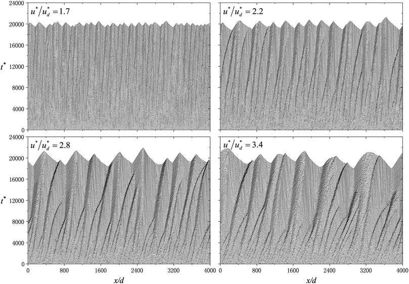
FIGURE 5. Space-time diagram of sand ripples’ development at four different wind velocities.

Figure 6A shows the growth curve of the ripple amplitude. To calculate the average amplitude, one should first cut the computational domain into slices along streamwise grid lines, deducing several cross sections. Then, we perform autocorrelation $C\left(\text{Δ}\lambda ,t\right)=\langle h\left(x,t\right)h\left(x+\text{Δ}\lambda ,t\right)\rangle -{\langle h\left(x,t\right)\rangle }^2$ on the ripple profiles of every cross section, averaging the results of all slices to get $\overline{C}\left(\text{Δ}\lambda ,t\right)$. Finally, the average amplitude A can be deduced from $A\left(t\right)=2\sqrt{2\overline{C}\left(0,t\right)}$. The linear stage is a period in which the amplitude A increases exponentially versus time. Small bumps rapidly emerge from the flat surface at this stage and immediately grow to regular ripples. After that, coarsening processes take over ripples’ development and slow down ripples’ growth on the amplitude.

FIGURE 6

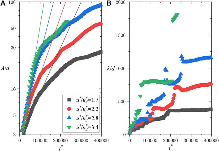
FIGURE 6. Time evolution of ripple amplitude (A) and wavelength (B) from the flat bed. Solid lines in (A) indicate the linear stage of ripple formation.

The x-coordinate value of the first peak on the $\overline{C}\left(\text{Δ}\lambda ,t\right)$ profile represents ripple wavelength λ at time t. As the results shown in Figure 6B indicate, there is a plateau in wavelength at the end of the linear stage for each wind velocity. According to Andreotti’s suggestion [5], this plateau indicates sand ripples’ initial wavelength ${\lambda }_{int}$. To avoid arbitrary treatment, in this work, we define ${\lambda }_{int}$ as the average wavelength in $t^{\text{*}}=100000\sim 150000$. This time period contains the previously mentioned plateau of all simulation cases. We compare the deduced ${\lambda }_{int}$ with the experimental result in Figure 7. For clearer comparison, we assume that all these wavelengths obey the scaling law introduced by Durán [12]. Then, they can be nondimensionalized as ${\lambda }_{int}^{\text{*}}={\lambda }_{int}g/\left(u_d^2\sqrt{{\rho }_f/{\rho }_p}\right)$. We find that ${\lambda }_{int}^{\text{*}}$ deduced from our model is very close to the experimental result, which grows linearly with frictional velocity and almost vanishes at $u^{\text{*}}=u_d^{\text{*}}$.

FIGURE 7

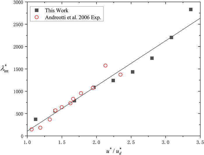
FIGURE 7. Initial wavelength ${\lambda }_{int}$ grows as a function of $u^{\text{*}}/u_d^{\text{*}}$ (solid symbols), compared with results from the wind tunnel experiment (hollow symbols). The solid line is the linear fitting of the simulation result.

After the linear stage, the ripples’ growth rate slows down. Checking the increase in wavelength in Figure 8, the simulation result of the wavelength exhibits a trending to a longer plateau, but generally, the growth rate of it holds as a constant. Wavelength data from field observations [38], from wind tunnel experiments [2, 5], and from continued models [9, 40] are consistent with the power law $\lambda \left(t\right)\propto t^{{\chi }_L}$, in which the growth rate $0.27<{\chi }_L<0.5$. ${\chi }_L$ in this work roughly fulfills this restriction and varies at the neighborhood around 0.5. Similar to experiments, ${\chi }_L$ increases slightly with $u^{\text{*}}$. However, this small increase is inconspicuous in this work. Amplitude grows coordinately with wavelength. Here, we check the ripple index (RI), which represents the ratio between wavelength and amplitude. The initial RI is a very large value with a quantity bigger than 100. During the linear stage, the RI decreases rapidly like it is shown in Figure 9 and eventually becomes a relatively constant value after regular ripples emerge. For aeolian ripples observed in the field, the RI usually ranges between 15 and 20 with a standard value of 18 for sand ripples and 15 for granule ripples [40]. This limitation roughly coincides with our RI results between $t^{\text{*}}=50000$ and $t^{\text{*}}=300000$, which are shown in the inset of Figure 9. For RIs deduced after $t^{\text{*}}=300000$, they become smaller than the expected value. It is because of the unstopped growth of the ripple amplitude, which will be discussed in the next section.

FIGURE 8

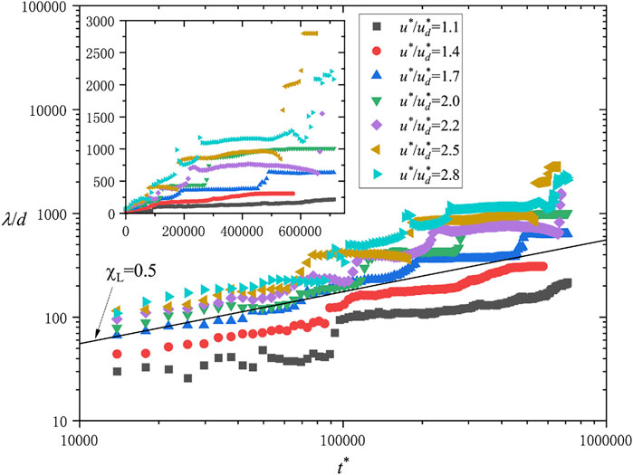
FIGURE 8. Development of ripple wavelength with time. The inset demonstrates the same result in the linear coordinate system. The black solid line illustrates the ${\chi }_L=0.5$ slope.

FIGURE 9

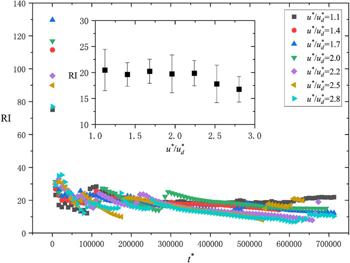
FIGURE 9. Ripple index (RI) development versus time. The inset shows the average value of the RI during $t^{\text{*}}=50000\sim 300000$ in different wind velocities.

3.2.2 Ripples Formed by Bidisperse Particles

Ripples’ growth rate should eventually become unperceivable after a long time of development. The existence of aeolian sand ripples’ saturated state has been proven by wind tunnel experiments [5]. In previous monodisperse cases, the simulation time is long enough to reach the saturated state. However, according to Figure 6, the “true” saturation has not been achieved at the end of the simulation. The incapability of reproducing the saturated bedform may be because of the lack of restriction on the increasing ripple scale. There are two plausible factors. The first one is that the homogeneous wind field used in this work cannot reproduce the complex distribution of ${\tau }_f$ near the surface after the ripple grows to a nonnegligible size. This treatment loses the retroactions from the bedform. The second one is that the monodisperse particle is unable to reproduce the particle size distribution on the bed surface and in the air. Experiments, observations, and theoretical models show that differences in particle size distribution influence aeolian sand ripples’ morphology [19, 25, 37].

The second imperfection can be conquered by using polydisperse particles. In this work, for simplicity, we use bidisperse particles to test the influence on ripple formation of particle size distribution. Similar to the computational settings in the last section, three cases with the same wind velocity are calculated under typical wind-blowing sand conditions. Case 1 is a monodisperse case with a particle diameter d which acts as a comparation. Case 2 is designed as a situation with an average diameter d. The diameter of those two kinds of particles used in case 2 are $d+d/2$ and $d-d/2$, respectively. Dynamic thresholds of particles in case 2 are all smaller than the given wind velocity. Case 3 is calculated with particles not smaller than d. The particle diameters in this case are d and $2.5d$. It represents the situation in which the coarser particles’ dynamic threshold cannot be reached by the wind field.

Ripples’ amplitude development in all three cases is demonstrated in Figure 10, in which variables are nondimensionalized by the average particle diameter $d_a$ of each case. From it, one will surprisingly find that the cases with bidisperse particles can reach a relatively steady amplitude after a distinct rapid growth stage. This phenomenon proves the assumption mentioned before that the armoring from the coarser particles contributes to the stabilization of the ripple morphology. Whether the coarser particles could be lifted by the splash process or not, the effect of armoring can always be observed on ripples’ development.

FIGURE 10

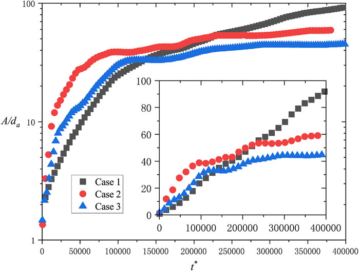
FIGURE 10. Time evolution on ripple amplitude of three different particle size distribution cases. The inset demonstrates the results in the linear coordinate system.

What is more, we can extract the average diameter distribution of surface particles as it is shown in Figure 11. D in it represents the local average diameter of particles on the bed surface. Particles in different sizes are regularly distributed in the computational domain for all bidisperse cases. Coarser particles prefer to gather on the crests of ripples. Meanwhile, fine particles tend to deposit on the trough. This coincides with the observation results from wind tunnel experiments and field observations.

FIGURE 11

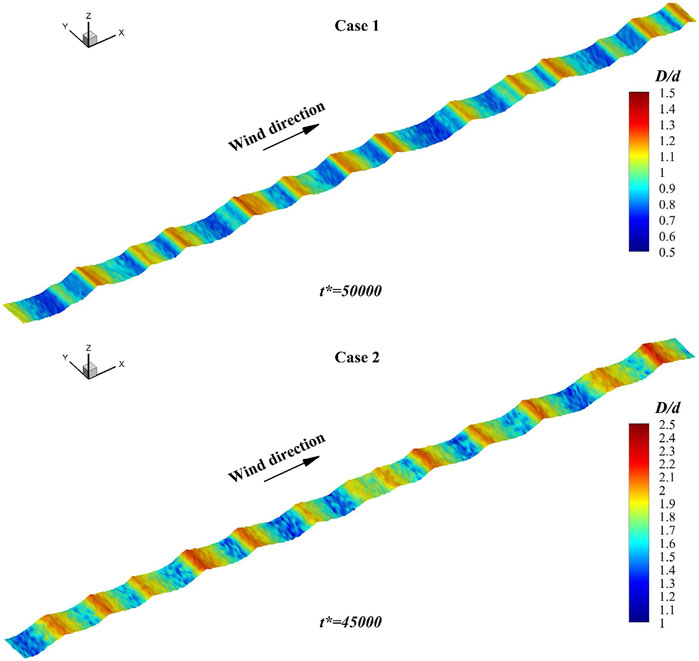
FIGURE 11. Size distribution of surface particles on ripple topography.

The general view on the mesoscopic particle dynamic during ripples’ development indicates that bigger particles are pushed to the crests because of the bombardment of saltating particles on the stoss slope. Our model has the ability to reproduce this process, which is very important for the simulation on some specific ripple forms, such as the so-called mega ripples.

3.2.3 Ripple Morphology in Transverse Direction

We can see from Figure 5 that larger ripples move slower, and smaller ones catch up and merge with them. Small bumps continually merge after their emergences. For a clearer observation, we run a wider monodisperse case, which is $4000d\times 800d\times 1200d$. This case is only run at one specific wind velocity.

Figure 12 shows the bedform topology from $t^{\text{*}}=20000$ to $t^{\text{*}}=80000$. The color represents the magnitude of $DR$, which stands for the deposition/erosion rate at that location, that is, $DR=\text{Δ}h\left(x,y\right)/\left(d\text{Δ}t\right)$. As we can see in these pictures, irregular structures gradually emerge from the flat surface and then strand to each other in the transverse direction, becoming relatively regular patterns. The initial wavelength appears very early at $t^{\text{*}}=40000$ while the bedform is chaotic in the 3D view. Amplitude growth slows down until $t^{\text{*}}=80000$ after recognizable ripples come out marking the end of the linear stage. However, ripples cannot become perfectly parallel lines after the linear stage in this wider computational domain. Defects such as disconnections and Y-shape branches arise just like features observed on the field or in the wind tunnel.

FIGURE 12

FIGURE 12. 3D view of aeolian sand ripple development.

Deposition and erosion are obviously influenced by the bedform. In Figure 13, by comparing the deposition/erosion rate in the dashed circles with the corresponding surface topology, one can see that before the bedform becomes regular, deposition frequently happens at the gap between staggered bumps, making them join together. At some locations, the deposition rate in the gaps is even bigger than those behind the adjacent bump. Then, as it is shown in Figure 12, on the ripple surface, deposition always takes place at the lee side, while erosions are all located at stoss slopes. From trough to crest, the erosion effect is reduced. It is because saltating particles bombard at the stoss slope, inducing reptating particles to climb up toward the crest. Near the top of the ripples, reptating particles jump over the ridge and deposit at the lee slope, making the deposition effect more remarkable close to the crest. This mechanism exists throughout the entire lifetime of sand ripples and motivates ripples to migrate along the wind direction.

FIGURE 13

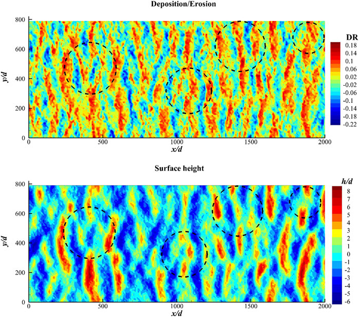
FIGURE 13. Comparison between the deposition/erosion rate and the corresponding surface topology in the same area.

3.3 Wind Profile Upon Ripple Surface

From the wind field profile corresponding to saturated aeolian sand transport, one can see whether the counter effect received from particles performs correctly. Meanwhile, differences of wind profile corresponding to various underlayer surfaces will be revealed. We will test the simulation performance on wind field calculation in this section. Although the fluid simulation in our model is simplified as a one-dimensional RANs problem, some average properties extracted from the simulation cases are still comparable with the experimental results.

The wind profiles on the flat surface and on the ripple surface are shown in Figure 14. Cases with the same s and $Ga$ in different wind velocities are picked out from pervious sections. The wind profile on the ripple surface is deduced from the wind field within the time period when the initial ripple emerges. The sand flux weakens the wind velocity near the sand bed. An obvious focal point deduced from the wind profile of the ripple surface indicates a constant height of the saltation layer for different wind velocities, which is also obtained from wind tunnel experiments [24]. Furthermore, when extracting the aerodynamic roughness $z_0$ from the wind profile far from the bed, as it is shown in the inset of Figure 14, $z_0$ can be fitted linearly. It means that $z_0$ fulfills the equation of constant focal point theory as shown below:

$z_0=z_F\text{exp}\left(\frac{-\kappa u_F}{u^{\text{*}}}\right),(32)$

where $z_F$ and $u_F$ are the height and wind velocity at the focal point, respectively. We can see that $z_F$ deduced from our model is very close to that from Ho’s experiment [15], while $u_F$ is closer to that in Durán’s DEM simulation result [10]. Since (32) is derived after taking the existence of a unique focal point as a prerequisite, this result also points to the constant height theory on the particle transport layer. In fact, according to the simulation results, (32) holds all the way during the ripples’ development process, which is shown in the inset of Figure 15.

FIGURE 14

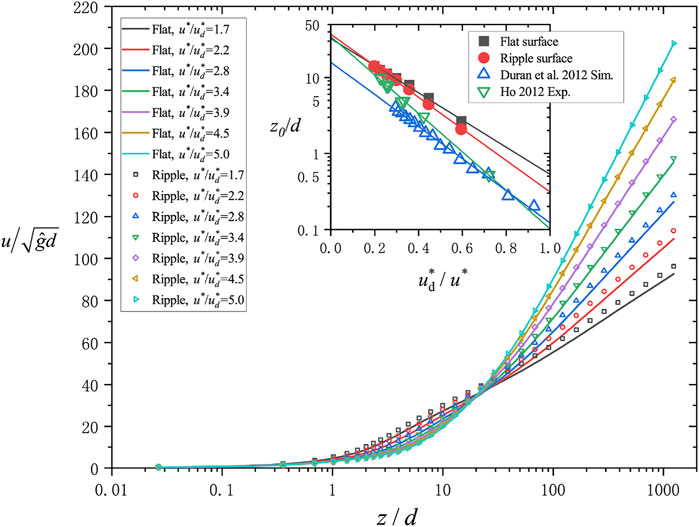
FIGURE 14. Wind profiles corresponding to saturated aeolian sand transport cases. The solid lines represent results on the flat surface. The scatter symbols are results from cases with the ripple surface. The inset demonstrates the relationship between $z_0$ and $u^{\text{*}}$. The hollow symbols in the inset represent results from others’ work.

FIGURE 15

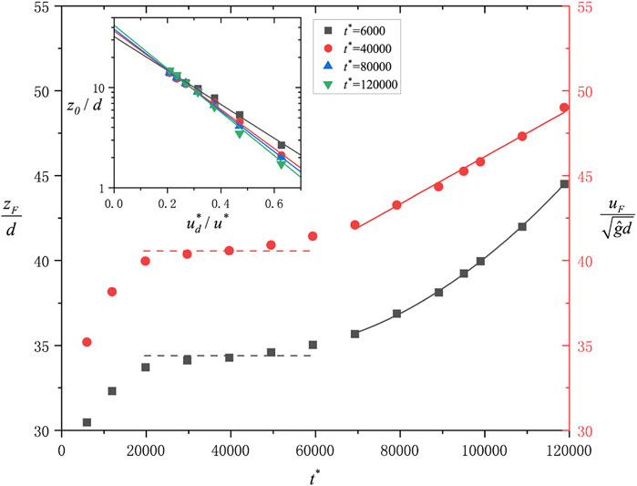
FIGURE 15. Time evolution on the height $z_F$ of the focal point and the wind velocity $u_F$ at this point. The inset shows the relationship between $z_0$ and $u^{\text{*}}$ at different times.

Comparing $z_0$ deduced on the ripple surface to those on the flat surface, it exhibits a slight decrease, especially for results at smaller wind velocities. As we know, in the presence of particle transport, the aerodynamic roughness $z_0$ deduced from the wind profile far from the bed has no relation to the topography of geometrical roughness and the size of the viscous sublayer. The main contributing factor to $z_0$ is particles’ trajectories. Thus, the counterintuitive decrease in $z_0$ for small wind velocities is not directly related to the surface topology but comes from the change of particles’ movement manner.

To study the statistical properties of bouncing particles’ trajectories, $z_F$ and $u_F$ are the values one should pay attention to. $z_F$ describes the bouncing height of particles, while $u_F$ reflects moving particles’ horizontal velocities. By implementing some simplification procedures, $z_F$ can be easily related to the average vertical initiating velocity of moving particles, which finally leads to a scaling law that $z_F\propto u_d^{\text{*}2}/g$. One can similarly express that $u_F$ as $u_F\propto u_d^{\text{*}}$ [11]. Figure 15 demonstrates the development of $z_F$ and $u_F$ versus time. From it, one can derive that from the flat surface to the surface with small bumps, the dynamic threshold $u_d^{\text{*}}$ performs a rapid increase. After reaching a specific value, $u_d^{\text{*}}$ roughly stays unchanged until ripple-like structures emerge at $t^{\text{*}}=60000$. Then, $u_d^{\text{*}}$ seems to increase linearly with time, which is reflected by the linear growth of $u_F$ and the quadratic increase of $z_F$.

This increase in $u_d^{\text{*}}$ is so small that it was usually ignored in former experimental works. However, there is some indirect evidence on this finding. Rasmussen and Mikkelsen observed the sand flux changing upon a pre-rippled sand bedform in a wind tunnel and found that the sand flux was constant during the first 30 min and then it decreased after 40 min. After 75 min, the flux had dropped to about 75% of the initial rate [29]. Starting with a flat surface, Rasmussen et al. found that the sand flux continuously decreases until the ripple surface develops to a steady state [30]. The total decrease quantity of mass flux in their work is between 75 and 90%. Similarly, in our monodisperse cases, we find that the sand flux decreases to about 80% of the initial value at $t^{\text{*}}=120000$. All these results may be caused by the small increase in $u_d^{\text{*}}$.

4 Discussion

The most distinct advantage of the methods used in this study compared with those of complete DEM simulations is the low-cost algorithm which makes it have the capability of simulating the aeolian particle transportation in more complex situations. Meanwhile, unlike continuous models, it maintains the conciseness of fundamental physical axioms while dealing with the vast amount of bouncing particle trajectories. This procedure avoids the arbitrary or oversimplified assumptions on saltation/depositing particles’ movement and leads to a more realistic vision of surface–particle interaction. As it was shown in the DEM simulation [12], we guarantee that the complexity of the particle trajectory will give the model an important ability to reproduce the collective processes during particle transport. The main idea behind establishing this numerical model is to inherit this kind of ability from the DEM and do our best to reduce the computational cost without showing too much influence on it. So, the key point is not simply lying on certain procedures but on the criteria deciding which part of the process should be simplified and how simplified it should be. From the results, we can see that the treatment in this work reaches a perfect balance point between the simplification on methods and the precision on results.

The flux result of this work can be perfectly fitted using Pähtz et al.’s unified expression, which is deduced from their own complete DEM model. This proves that our model has successfully maintained the primary characteristics of the particle motion. Hence, it could be a useful tool in the research of sand flux property upon the ripple surface in the future, taking the research on the saturation length of sand transport as an example. Although there is an excellent theoretical work which presents a very accurate model for the saturation length, it is just over a flat erodible soil [27]. By using our model, one will have the ability to quantify the saturation length as a function of the bedform topography and particle properties, which is very important for the research of mega ripples and dunes. Compared to the complete DEM model, our model has a clear-cut definition of particle status. There are no blur definitions in this model between the moving particles and the static bed. Meanwhile, the simplicity of it allows us to add more complex mechanisms into the model to study more influential aspects of the sediment transport, such as complex turbulence structures or the cohesion.

This model reproduces the morphology development of aeolian sand ripples qualitatively and quantitatively. The relationship between ripple wavelength and wind velocity fits well with the wind tunnel experiment data. What is more, due to the simplified treatment on particle size distribution calculation, one can deduce the final stable wavelength of aeolian sand ripples, which has not been deduced using any direct simulation models before.

The inverse grading in aeolian ripples has been reproduced as well. Although Anderson and Bunas studied this phenomenon using their cellular automaton model [3], some new results can be deduced from our novel model in the future. This is because compared to the automaton model, our model has realistic saltation trajectories, while the cellular automaton model simplifies the saltating particles as a series of randomly distributed impact beans. Durán et al. found that the trajectories of saltating particles can be modulated by the wavy surface [12]. These resonant saltation trajectories contain the information of the ripples’ geometric scale. On the other hand, our model can calculate polydisperse problems with arbitrary particle size distribution. This advantage gives us an easier way to perform careful research on the relationship between the inverse grading and the particle size distribution of the original bed.

This model provides a 3D view on observing ripple formation. Small bumps merge with each other and migrate along the wind direction as soon as they emerge from the flat bed. It is caused by the inhomogeneous distribution of the erosion/deposition region. Deposition always happens at the lee side of ripples, while erosion takes place at the stoss side.

Lastly, by testing the wind profile on the flat surface and on the ripple surface, we find that this model can simulate the average wind field on the ripple surface as well. It reproduces the focal point of different wind profiles and shows the development of particle transportation during bed form deformation. The dynamic threshold of bouncing particles increases to a certain value and holds at it at the early stage of ripple formation. Then, it increases linearly with time after the initial ripple is formed.

This model performs well on simulating aeolian sand ripples’ development on Earth. Furthermore, since all equations contained in this model are derived from basic physical laws, it can be directly used in the research studies on planetary geomorphology as well. However, due to the simplification on the wind field and the surface particle size distribution, this model cannot deal with big structures such as meter-scale mega ripples and kilometer-scale sand dunes because we believe that the big-scale turbulence structure may affect the particle trajectory profoundly. Expecting this model to be the most feasible method to reveal the immanent properties of mega ripples in planetary geography research, we will continually improve it in future works.

Data Availability Statement

The raw data supporting the conclusions of this article will be made available by the authors, without undue reservation.

Author Contributions

XH contributed to the conception and proposed the code design in this study. All authors made contributions to the result and analysis and the construction of the manuscript.

Funding

This work is supported by the State Key Program of the National Natural Science Foundation of China (41931179), the National Natural Science Foundation of China (11772143, 11702163), and the Key Research and Development Program of Ningxia (2018BFH03004).

Conflict of Interest

The authors declare that the research was conducted in the absence of any commercial or financial relationships that could be construed as a potential conflict of interest.

Acknowledgments

We thank the reviewers for constructive comments and suggestions.

References

1. Anderson RS. A Theoretical Model for Aeolian Impact Ripples. Sedimentology (1987) 34:943–56. doi:10.1111/j.1365-3091.1987.tb00814.x

CrossRef Full Text | Google Scholar

2. Anderson R. Eolian Ripples as Examples of Self-Organization in Geomorphological Systems. Earth-Science Rev (1990) 29:77–96. doi:10.1016/0012-8252(0)90029-U

CrossRef Full Text | Google Scholar

3. Anderson RS, Bunas KL. Grain Size Segregation and Stratigraphy in Aeolian Ripples Modelled with a Cellular Automaton. Nature (1993) 365:740–3. doi:10.1038/365740a0

CrossRef Full Text | Google Scholar

4. Anderson RS, Haff PK. Wind Modification and Bed Response during Saltation of Sand in Air. In: OE Barndorff-Nielsen, and BB Willetts, editors. Aeolian Grain Transport 1. Vienna: Springer (1991). p. 21–51. doi:10.1007/978-3-7091-6706-9_2

CrossRef Full Text | Google Scholar

5. Andreotti B, Claudin P, Pouliquen O. Aeolian Sand Ripples: Experimental Study of Fully Developed States. Phys Rev Lett (2006) 96:028001. doi:10.1103/PhysRevLett.96.028001

PubMed Abstract | CrossRef Full Text | Google Scholar

6. Bagnold RA. Physics of Blown Sand and Desert Dunes. New York: W. Morrow & company (1942).

7. Brilliantov NV, Pöschel T. Kinetic Theory of Granular Gases. Oxford: Oxford University Press (2010).

8. Creyssels M, Dupont P, El Moctar AO, Valance A, Cantat I, Jenkins JT, et al. Saltating Particles in a Turbulent Boundary Layer: Experiment and Theory. J Fluid Mech (2009) 625:47–74. doi:10.1017/S0022112008005491

CrossRef Full Text | Google Scholar

9. Csahók Z, Misbah C, Rioual F, Valance A. Dynamics of Aeolian Sand Ripples. The Eur Phys J E (2000) 3:71–86. doi:10.1007/s101890070043

CrossRef Full Text | Google Scholar

10. Durán O, Andreotti B, Claudin P. Numerical Simulation of Turbulent Sediment Transport, from Bed Load to Saltation. Phys Fluids (2012) 24:103306. doi:10.1063/1.4757662

CrossRef Full Text | Google Scholar

11. Durán O, Claudin P, Andreotti B. On Aeolian Transport: Grain-Scale Interactions, Dynamical Mechanisms and Scaling Laws. Aeolian Res (2011) 3:243–70. doi:10.1016/j.aeolia.2011.07.006

CrossRef Full Text | Google Scholar

12. Durán O, Claudin P, Andreotti B. Direct Numerical Simulations of Aeolian Sand Ripples. Proc Natl Acad Sci (2014) 111:15665–8. doi:10.1073/pnas.1413058111

PubMed Abstract | CrossRef Full Text | Google Scholar

13. Ferguson RI, Church M. A Simple Universal Equation for Grain Settling Velocity. J Sediment Res (2004) 74:933–7. doi:10.1306/051204740933

CrossRef Full Text | Google Scholar

14. Fohanno S, Oesterlé B. Analysis of the Effect of Collisions on the Gravitational Motion of Large Particles in a Vertical Duct. Int J multiphase flow (2000) 26:267–92. doi:10.1016/S0301-9322(99)00005-1

CrossRef Full Text | Google Scholar

15. Ho T-D. Etude expérimentale du transport de particules dans une couche limite turbulente. Ph.D. thesis. Rennes: University of Rennes (2012).

Google Scholar

16. Ho TD, Valance A, Dupont P, Ould El Moctar A. Scaling Laws in Aeolian Sand Transport. Phys Rev Lett (2011) 106:094501. doi:10.1103/PhysRevLett.106.094501

PubMed Abstract | CrossRef Full Text | Google Scholar

17. Hoyle RB, Woods AW. Analytical Model of Propagating Sand Ripples. Phys Rev E (1997) 56:6861–8. doi:10.1103/PhysRevE.56.6861

CrossRef Full Text | Google Scholar

18. Iversen JD, Rasmussen KR. The Effect of Wind Speed and Bed Slope on Sand Transport. Sedimentology (1999) 46:723–31. doi:10.1046/j.1365-3091.1999.00245.x

CrossRef Full Text | Google Scholar

19. Katra I, Yizhaq H. Intensity and Degree of Segregation in Bimodal and Multimodal Grain Size Distributions. Aeolian Res (2017) 27:23–34. doi:10.1016/j.aeolia.2017.05.002

CrossRef Full Text | Google Scholar

20. Kawamura R. Study on Sand Movement by Wind. Rept Inst Sci Technol (1951) 5:95–112.

Google Scholar

21. Kok JF, Renno NO. A Comprehensive Numerical Model of Steady State Saltation (Comsalt). J Geophys Res (2009) 114, D17204. doi:10.1029/2009JD011702

CrossRef Full Text | Google Scholar

22. Lämmel M, Dzikowski K, Kroy K, Oger L, Valance A. Grain-scale Modeling and Splash Parametrization for Aeolian Sand Transport. Phys Rev E (2017) 95:022902. doi:10.1103/PhysRevE.95.022902

PubMed Abstract | CrossRef Full Text | Google Scholar

23. Lämmel M, Kroy K. Analytical Mesoscale Modeling of Aeolian Sand Transport. Phys Rev E (2017) 96:052906. doi:10.1103/PhysRevE.96.052906

PubMed Abstract | CrossRef Full Text | Google Scholar

24. Martin RL, Kok JF. Wind-invariant Saltation Heights Imply Linear Scaling of Aeolian Saltation Flux with Shear Stress. Sci Adv (2017) 3:e1602569. doi:10.1126/sciadv.1602569

PubMed Abstract | CrossRef Full Text | Google Scholar

25. McKenna Neuman C, Bédard O. A Wind Tunnel Investigation of Particle Segregation, Ripple Formation and Armouring within Sand Beds of Systematically Varied Texture. Earth Surf Process Landforms (2017) 42:749–62. doi:10.1002/esp.4019

CrossRef Full Text | Google Scholar

26. Pähtz T, Durán O. Unification of Aeolian and Fluvial Sediment Transport Rate from Granular Physics. Phys Rev Lett (2020) 124:168001. doi:10.1103/PhysRevLett.124.168001

PubMed Abstract | CrossRef Full Text | Google Scholar

27. Pähtz T, Parteli EJR, Kok JF, Herrmann HJ. Analytical Model for Flux Saturation in Sediment Transport. Phys Rev E (2014) 89:052213. doi:10.1103/PhysRevE.89.052213

CrossRef Full Text | Google Scholar

28. Prigozhin L. Nonlinear Dynamics of Aeolian Sand Ripples. Phys Rev E (1999) 60:729–33. doi:10.1103/PhysRevE.60.729

CrossRef Full Text | Google Scholar

29. Rasmussen KR, Mikkelsen HE. Wind Tunnel Observations of Aeolian Transport Rates. In: OE Barndorff-Nielsen, and BB Willetts, editors. Aeolian Grain Transport 1. Vienna: Springer (1991). p. 135–44. doi:10.1007/978-3-7091-6706-9_8

CrossRef Full Text | Google Scholar

30. Rasmussen KR, Valance A, Merrison J. Laboratory Studies of Aeolian Sediment Transport Processes on Planetary Surfaces. Geomorphology (2015) 244:74–94. doi:10.1016/j.geomorph.2015.03.041

CrossRef Full Text | Google Scholar

31. Schwager T, Becker V, Pöschel T. Coefficient of Tangential Restitution for Viscoelastic Spheres. Eur Phys J E (2008) 27:107–14. doi:10.1140/epje/i2007-10356-3

PubMed Abstract | CrossRef Full Text | Google Scholar

32. Shao Y, Lu H. A Simple Expression for Wind Erosion Threshold Friction Velocity. J Geophys Res (2000) 105:22437–43. doi:10.1029/2000JD900304

CrossRef Full Text | Google Scholar

33. Sharp RP. Wind Ripples. J Geology (1963) 71:617–36. doi:10.1086/626936

CrossRef Full Text | Google Scholar

34. Valance A, Rioual F. A Nonlinear Model for Aeolian Sand Ripples. Eur Phys J B (1999) 10:543–8. doi:10.1007/s100510050884

CrossRef Full Text | Google Scholar

35. Versteeg HK, Malalasekera W. An Introduction to Computational Fluid Dynamics: The Finite Volume Method. Harlow, UK: Pearson Education (2007).

36. Walker JD. An Experimental Study of Wind Ripples. Ph.D. thesis. Cambridge: Massachusetts Institute of Technology (1981).

37. Wang P, Zhang J, Huang N. A Theoretical Model for Aeolian Polydisperse-Sand Ripples. Geomorphology (2019) 335:28–36. doi:10.1016/j.geomorph.2019.03.013

CrossRef Full Text | Google Scholar

38. Werner BT, Gillespie DT. Fundamentally Discrete Stochastic Model for Wind Ripple Dynamics. Phys Rev Lett (1993) 71:3230–3. doi:10.1103/PhysRevLett.71.3230

PubMed Abstract | CrossRef Full Text | Google Scholar

39. Yin X, Huang N, Jiang C, Parteli EJR, Zhang J. Splash Function for the Collision of Sand-Sized Particles onto an Inclined Granular Bed, Based on Discrete-Element-Simulations. Powder Tech (2021) 378:348–58. doi:10.1016/j.powtec.2020.10.008

CrossRef Full Text | Google Scholar

40. Yizhaq H, J. Balmforth N, Provenzale A. Blown by Wind: Nonlinear Dynamics of Aeolian Sand Ripples. Physica D: Nonlinear Phenomena (2004) 195:207–28. doi:10.1016/j.physd.2004.03.015

CrossRef Full Text | Google Scholar