Event-Chain Monte Carlo: Foundations, Applications, and Prospects

1. Introduction

Markov-chain Monte Carlo (MCMC) is an essential tool for the natural sciences. It is also the subject of a research discipline in mathematics. Ever since its invention, in 1953, MCMC [1] has focused on reversible MCMC algorithms, those that satisfy a detailed-balance condition. These algorithms are particularly powerful when the Monte Carlo moves (from one configuration to the next), and they can be customized for each configuration of a given system. Such a priori choices [2] allow for big moves to be accepted and for sample space to be explored rapidly. Prominent examples for reversible methods with custom-built, large-scale moves are path-integral Monte Carlo and the cluster algorithms for spin systems [3].

In many important problems, insightful a priori choices for moves are yet unavailable. MCMC then often consists of a sequence of unbiased local moves, such as tiny displacements of one out of N particles, or flips of one spin out of many. Local reversible Monte Carlo schemes are easy to set up for these problems. The Metropolis or the heatbath (Gibbs-sampling) algorithms are popular choices. They generally compute acceptance probabilities from the changes in the total potential (the system's energy) and thus mimic the behavior of physical systems in the thermodynamic equilibrium. However, such algorithms are often too slow to be useful. Examples are the hard-disk model [4, 5] where local reversible MCMC methods failed for several decades to obtain independent samples in large systems, and the vast field of molecular simulation [6], which considers classical models of polymers, proteins, etc., in aqueous solution. Local reversible MCMC algorithms were for a long time without alternatives in molecular simulation, but they remained of little use because of their lack of efficiency.

Event-chain Monte Carlo (ECMC) [7, 8] is a family of local, non-reversible MCMC algorithms developed over the last decade. Its foundations, applications, and prospects are at the heart of the present review. At a difference with its local reversible counterparts (that are all essentially equivalent to each other and to the physical overdamped equilibrium dynamics), different representatives of ECMC present a wide spread of behaviors for a given model system. Two issues explain this spread. First, any decision to accept or reject a move is made on the basis of a multitude of statistically independent decisions of parts of the systems, so-called factors (see the Glossary). Usually, there is a choice between inequivalent factorizations. In the Metropolis algorithm, in contrast, all decisions to accept a move are made on the basis of changes in the total energy. Second, ECMC is fundamentally a non-reversible “lifted” version of an underlying reversible algorithm. In a lifting (a lifted Markov chain), some of the randomly sampled moves of the original (“collapsed”) Markov chain are rearranged. Again, there are many possible liftings and each of these can give rise to a specific dynamic behavior. The development of ECMC is still in its infancy. Its inherent variability may, however, bring to life the use of local MCMC in the same way as reversible energy-based Monte Carlo has been empowered through the a priori probabilities.

Section 2 discusses the mathematical foundations underlying ECMC, namely global balance, factorization, liftings, and thinning (making statistically correct decisions with minimal effort). Section 3 reviews exact results for various Markov chains in the simplest setting of a path graph. Section 4 studies one-dimensional N-body systems. Section 5 provides an overview of findings on N-particle systems in higher than one dimension. Section 6 reviews a recent proposal to apply ECMC to molecular simulations. Section 7, finally, discusses prospects for event-chain Monte Carlo and other non-reversible Markov chains in the context of molecular simulation. The Glossary contains non-technical introductions to the main terms used in this review.

2. Markov Chains, Factorization, Liftings, and Thinning

The present section reviews fundamentals of ECMC. Non-reversibility modifies the positioning of MCMC from an analog of equilibrium physics toward the realization of a non-equilibrium system with steady-state flows. Section 2.1 discusses transition matrices, the objects that express MCMC algorithms in mathematical terms. The balance conditions for the steady state of Markov chains are reviewed, as well as the performance limits of MCMC in terms of basic characteristics of the sample space and the transition matrix. Section 2.2 discusses factorization, the break-up of the interaction into terms that, via the factorized Metropolis algorithm, make independent decisions on the acceptance or the rejection of a proposed move. Section 2.3 reviews the current understanding of lifted Markov chains, the mathematical concept used by ECMC to replace random moves by deterministic ones without modifying the stationary distribution. This remains within the framework of (memory-less) Markov chains. Section 2.4 reviews thinning, the way used in ECMC to make complex decisions with minimum computations.

2.1. Transition Matrices and Balance Conditions

For a given sample space Ω, a Markov chain essentially consists in a time-independent transition matrix P and a distribution of initial configurations. Any non-negative element P_ij gives the conditional probability for the configuration i to move to configuration j in one time step. The transition matrix P is stochastic—all its rows i sum up to $\sum _{j\in \Omega }{P}_{ij}=1$. Commonly, the probability P_ij is composed of two parts $P_{ij}={{A}}_{ij}{{P}}_{ij}$, where ${A}$ is the a priori probability to propose a move (mentioned in section 1), and ${{P}}_{ij}$ the so-called “filter” to accept the proposed move. Any term P_ii in the transition matrix is the probability to move from i to i. If non-vanishing, it may result from the probability of all proposed moves from i to other configurations j ≠ i (by the a priori probability) to be rejected (by the filter ${P}$). In the lifted sample space $\widehat{\Omega }$ that will be introduced in subsection 2.3, ECMC is without rejections.

2.1.1. Irreducibility and Convergence—Basic Properties of the Transition Matrix

A (finite) Markov chain is irreducible if any configuration j can be reached from any other configuration i in a finite number of time steps [9, section 1.3]. As the matrix $P^t={(P^t)}_{ij}$ gives the conditional probability to move from i to j in exactly t time steps, an irreducible matrix has ${(P^t)}_{ij}>0$ ∀i, j, but the time t may depend on i and j.

The transition matrix P connects not only configurations but also probability distributions π^{t−1} and π^{t} at subsequent time steps t − 1 and t. By extension, the matrix P^t connects the distribution π^{t} with the (user-provided) distribution of initial configurations π^{0} at time t = 0:

$\begin{array}{ll}{\pi }_i^{\left\{t\right\}}={\displaystyle \sum _{j\in \Omega }}{\pi }_j^{\left\{t-1\right\}}{P}_{ji}\Rightarrow {\pi }_i^{\left\{t\right\}}={\displaystyle \sum _{j\in \Omega }}{\pi }_j^{\left\{0\right\}}{(P^t)}_{ji}\forall i\in \Omega .& (1)\end{array}$

The initial distribution π^{0} can be concentrated on a single initial configuration. In that case, π^{0} is a discrete Kronecker δ-function for a Markov chain in a finite sample space, and a Dirac δ-function in a continuous sample space.

An irreducible Markov chain has a unique stationary distribution π that satisfies

$\begin{array}{ll}{\pi }_i={\displaystyle \sum _{j\in \Omega }}{\pi }_j{P}_{ji}\forall i\in \Omega .& (2)\end{array}$

Equation (2) allows one to define the flow ${{F}}_{ji}$ from j to i as the stationary probability π_j to be at j multiplied with the conditional probability to move from j to i:

$\begin{array}{r}{{F}}_{ji}\equiv {\pi }_j{P}_{ji}\Rightarrow \text{\hspace{1em}Equation}(2)\iff {\pi }_i=\stackrel{\text{flows exiting }i}{\overbrace{{\displaystyle \sum _{k\in \Omega }}{{F}}_{ik}}}\\ =\stackrel{\text{flows entering }i}{\overbrace{{\displaystyle \sum _{j\in \Omega }}{{F}}_{ji}}}\forall i\in \Omega ,& (3)\end{array}$

where the left-hand side of Equation (2) was multiplied with the stochasticity condition $\sum _{k\in \Omega }{P}_{ik}=1$.

Although any irreducible transition matrix has a unique π, this distribution is not guaranteed to be the limit π^{t} for t → ∞ for all initial distributions π^{0}. But even in the absence of convergence, ergodicity follows from irreducibility alone, and ensemble averages $\sum _{i\in \Omega }{O}(i){\pi }_i$ of an observable ${O}$ agree with the time averages ${lim}_{t\to \infty }\frac{1}{t}\sum _{s=0}^{t-1}{O}(i_s)$ (see [9, Theorem 4.16]).

Convergence toward π of an irreducible Markov chain requires that it is aperiodic, i.e., that the return times from a configuration i back to itself $\left\{t\ge 1:{(P^t)}_{ii}>0\right\}$ are not all multiples of a period larger than one. For example, if the set of return times is {2, 4, 6, …}, then the period is 2, but if it is {1000, 1001, 1002, …}, then it is 1. These periods do not depend on the configuration i. For irreducible, aperiodic transition matrices, $P^t={(P^t)}_{ij}$ is a positive matrix for some fixed t, and MCMC converges toward π from any starting distribution π^{0}. The existence and uniqueness of the stationary distribution π follows from the irreducibility of the transition matrix, but if its value is imposed (for example to be the Boltzmann distribution or the diagonal density matrix [3]), then Equation (2) becomes a necessary “global-balance” condition for the transition matrix. For ECMC, this global-balance condition of Equation (2) must be checked for all elements of the lifted sample space $\widehat{\Omega }$.

A reversible transition matrix is one that satisfies the detailed-balance condition

$\begin{array}{ll}{{F}}_{ij}=\stackrel{\text{flow from }i\text{ to }j}{\overbrace{{\pi }_i{P}_{ij}}}=\stackrel{\text{flow from }j\text{ to }i}{\overbrace{{\pi }_j{P}_{ji}}}={{F}}_{ji}\forall i,j\in \Omega .& (4)\end{array}$

Detailed balance implies global balance (Equation 4 yields Equation 2 by summing over j, considering that $\sum _{j\in \Omega }{P}_{ij}=1$), and the flow into a configuration i coming from a configuration j goes right back to j. In ECMC, the reality of the global-balance condition is quite the opposite, because the entering flow ${{F}}_{ji}$ is compensated by flows to other configurations than j (${{F}}_{ji}>0$ usually implies ${{F}}_{ij}=0$). Checking the global-balance condition is more complicated than checking detailed balance, as it requires monitoring all the configurations j that contribute to the flow into i, in a larger (lifted) sample space.

For a reversible Markov chain, the matrix $A_{ij}={\pi }_i^{1/2}{P}_{ij}{\pi }_j^{-1/2}$ is symmetric, as trivially follows from the detailed-balance condition. The spectral theorem then assures that A has only real eigenvalues and that its eigenvectors form an orthonormal basis. The transition matrix P has the same eigenvalues as A, as well as closely related eigenvectors:

$\begin{array}{l}{\displaystyle \sum _{j\in \Omega }}{\displaystyle \underset{A_{ij}}{{\displaystyle \underbrace{{\pi }_i^{1/2}{P}_{ij}{\pi }_j^{-1/2}}}}}{x}_j=\lambda x_i\iff \\ {\displaystyle \sum _{j\in \Omega }}{P}_{ij}{\displaystyle \underset{{\tilde{x}}_j}{{\displaystyle \underbrace{\left[{\pi }_j^{-1/2}{x}_j\right]}}}}=\lambda {\displaystyle \underset{{\tilde{x}}_i}{{\displaystyle \underbrace{\left[{\pi }_i^{-1/2}{x}_i\right]}}}}.& (5)\end{array}$

The eigenvectors $\tilde{x}$ of P must be multiplied with $\sqrt{\pi }$ to be mutually orthogonal. They provide a basis on which any initial probability distribution π^{0} can be expanded. An irreducible and aperiodic transition matrix P (reversible or not) has one eigenvalue λ₁ = 1, and all others satisfy |λ_k| < 1 ∀k ≠ 1. The unit eigenvalue λ₁ corresponds to a constant right eigenvector of P because of the stochasticity condition $\sum _{j\in \Omega }{P}_{ij}=1$, and to the left eigenvector π of P, because of the global-balance condition of Equation (2).

A non-reversible transition matrix may belong to a mix of three different classes, and this variety greatly complicates their mathematical analysis. P may have only real eigenvalues and real-valued eigenvectors, but without there being an associated symmetric matrix A, as in Equation (5) (see [10, section 2.3] for an example). A non-reversible transition matrix may also have only real eigenvalues but with geometrical multiplicities that not all agree with the algebraic multiplicities. Such a matrix is not diagonalizable. Finally, P may have real and then pairs of complex eigenvalues [10]. This generic transition matrix can be analyzed in terms of its eigenvalue spectrum, and expanded in terms of a basis of eigenvectors [11–13]. As non-reversible transition matrices may well have only real eigenvalues, the size of their imaginary parts does not by itself indicate the degree of non-reversibility [14]. Reversibilizations of non-reversible transition matrices have been much studied [15], but they modify the considered transition matrix.

2.1.2. Total Variation Distance, Mixing Times

In real-world applications, irreducibility and aperiodicity of a Markov chain can usually be established beyond doubt. The stationary distribution π of a transition matrix constructed to satisfy a global-balance condition is also known explicitly. The time scale for the exponential approach of π^{t} to π—that always exists—is much more difficult to establish. In principle, the difference between the two distributions is quantified through the total variation distance:

$\begin{array}{ll}||{\pi }^{\left\{t\right\}}-\pi |{|}_{\text{TV}}={\displaystyle \underset{A\subset \Omega }{max}}|{\pi }^{\left\{t\right\}}(A)-\pi (A)|=\frac{1}{2}{\displaystyle \sum _{i\in \Omega }}|{\pi }_i^{\left\{t\right\}}-{\pi }_i|.& (6)\end{array}$

The distribution π^{t} depends on the initial distribution, but for any choice of π^{0}, for an irreducible and aperiodic transition matrix, the total variation distance is smaller than an exponential bound Cα^t with α ∈ (0, 1) (see the convergence theorem for Markov chains [9, Theorem 4.9]). At the mixing time, the distance from the most unfavorable initial configuration,

$\begin{array}{ll}d(t)={\displaystyle \underset{{\pi }^{\left\{0\right\}}}{max}}||{\pi }^{\left\{t\right\}}({\pi }^{\left\{0\right\}})-\pi |{|}_{\text{TV}},& (7)\end{array}$

drops below a certain value ϵ

$\begin{array}{ll}{t}_{\text{mix}}(ϵ)=min\left\{t:d(t)\le ϵ\right\}.& (8)\end{array}$

Usually, $ϵ=\frac{1}{4}$ is taken, with t_mix = t_mix(1/4) (see [9]). The value of ϵ is arbitrary, but smaller than 1/2 in order for convergence in a small part of Ω (without exploration of its complement) not to be counted as a success (see subsection 3.2.1 for an example). Once such a value smaller than $\frac{1}{2}$ is reached, exponential convergence in t/t_mix sets in (see [9, Equation 4.36]). The mixing time is thus the time to obtain a first sample of the stationary distribution from a most unfavorable initial configuration. It does not require the existence of a spectrum of the transition matrix P, and it can be much larger than the correlation time t_corr given by the absolute inverse spectral gap of P, if it exists (the time it takes to decorrelate samples in the stationary regime). Related definitions of the mixing time take into account such thermalized initial configurations [16].

2.1.3. Diameter Bounds, Bottleneck, Conductance

An elementary lower bound for the mixing time on a graph G = (Ω, E) (with the elements of Ω as vertices, and the non-zero elements of the transition matrix as edges) is given by the graph diameter L_G, that is, the minimal number of time steps it takes to connect any two vertices i, j ∈ Ω. The mixing time, for any ϵ < 1/2, trivially satisfies

$\begin{array}{ll}{t}_{\text{mix}}\ge \frac{L_G}{2}.& (9)\end{array}$

For the Metropolis or heatbath single-spin flip dynamics in the Ising model with N spins (in any dimension D), mixing times throughout the high-temperature phase are logarithmically close to the diameter bound with the graph diameter L_G = N, the maximum number of spins that differ between i and j (see [17]).

Mixing and correlation times of a MCMC algorithm can become very large if there is a bottleneck in the sample space Ω. Two remarkable insights are that in MCMC there is but a single such bottleneck (rather than a sequence of them), and that the mixing time is bracketed (rather than merely bounded from below) by functions of the conductance [18]. Also called “bottleneck ratio” [9] or “Cheeger constant” [19], the conductance is defined as the flow across the bottleneck:

$\begin{array}{ll}\Phi \equiv {\displaystyle \underset{S\subset \Omega ,{\pi }_S\le \frac{1}{2}}{min}}\frac{{{F}}_{S\to \overline{S}}}{{\pi }_S}={\displaystyle \underset{S\subset \Omega ,{\pi }_S\le \frac{1}{2}}{min}}\frac{{\displaystyle {\sum }_{i\in S,j\in \overline{S}}}{\pi }_i{P}_{ij}}{{\pi }_S},& (10)\end{array}$

where $\overline{S}=\Omega \backslash S$. Although it can usually not be computed in real-world applications, the conductance is of importance because the liftings which are at the heart of ECMC leave it unchanged (see subsection 2.3).

For reversible Markov chains, the correlation time is bounded by the conductance as [18]:

$\begin{array}{ll}\frac{1}{\Phi }\le t_{\text{corr}}\le \frac{8}{{\Phi }^2}.& (11)\end{array}$

The lower bound follows from the fact that to cross from S into $\overline{S}$, the Markov chain must pass through the boundary of S, but this cannot happen faster than through direct sampling within S, i.e., with probability π_i/π_S for i on the boundary of S. The upper bound was proven in [20, Lemma 3.3]. For arbitrary MCMC, one has the relation

$\begin{array}{ll}\frac{1}{4\Phi }\le t_{\text{set}}\le \frac{20}{{\Phi }^2},& (12)\end{array}$

where t_set is the “set time,” the maximum over all sets S of the expected time to hit a set S from a configuration sampled from π, multiplied with the stationary distribution π(S). In addition, the mixing time, defined with the help of a stopping rule [18], satisfies:

$\begin{array}{ll}\frac{\text{const}}{\Phi }<t_{\text{mix}}<\frac{{\text{const}}^{\prime }}{{\Phi }^2}log\frac{1}{{\pi }_{min}},& (13)\end{array}$

where the constants are different for reversible and for non-reversible Markov chains, and π_min is the smallest weight of all configurations.

The above inequalities strictly apply only to finite Markov chains, where the smallest weight π_min of all configurations is well-defined. A continuous system may have to be discretized in order to allow a discussion in its terms. Also, in the application to ECMC, which is event-driven, mixing and correlation times may not reflect computational effort, which roughly corresponds to the number of events, rather than of time steps. Nevertheless, the conductance yields the considerable diffusive-to-ballistic speedup that may be reached by a non-reversible lifting (see [18]) if the collapsed Markov chain is itself close to the ~ 1/Φ² upper bound of Equations (11) and (13).

2.2. Factorization

In generic MCMC, each proposed move is accepted or rejected based on the change in total potential that it entails. For hard spheres, a move in the Metropolis algorithm [3, Chapter 2] can also be pictured as being accepted “by consensus” over all pairs of spheres (none of which may present an overlap) or else rejected “by veto” of at least one pair of spheres (the pair which presents an overlap). The “potential landscape” and the “consensus–veto” interpretations are here equivalent as the pair potential of two overlapping hard spheres is infinite, and therefore also the total potential as soon as there is one such pair.

The factorized Metropolis filter [8, 21] generalizes the “consensus–veto” picture to an arbitrary system whose stationary distribution breaks up into a set ${M}$ of factors M = (I_M, T_M). Here, I_M is an index set and T_M a type (or label), such as “Coulomb,” “Lennard-Jones,” “Harmonic” (see [21, section 2A]). The total potential U of a configuration c then writes as the sum over factor potentials U_M that only depend on the factor configurations c_M:

$\begin{array}{ll}U({\displaystyle \underset{c}{{\displaystyle \underbrace{\{{\text{r}}_1,\dots ,{\text{r}}_N\}}}}})={\displaystyle \sum _{M\in {M}}}{U}_M({\displaystyle \underset{c_M}{{\displaystyle \underbrace{\{{\text{r}}_i:i\in I_M\}}}}}),& (14)\end{array}$

and the stationary distribution appears as a product over exponentials of factor potentials:

$\begin{array}{r}\pi (c)=exp\left[-\beta U(c)\right]={\displaystyle \prod _{M\in {M}}}{\pi }_M(c_M)\\ ={\displaystyle \prod _{M\in {M}}}exp\left[-\beta U_M(c_M)\right],& (15)\end{array}$

where β is the inverse temperature. Energy-based MCMC considers the left-hand side of Equation (14) and molecular dynamics its derivatives (the forces on particles). All factorizations ${M}$ are then equivalent. In contrast, ECMC concentrates on the right-hand side of Equation (14), and different factorizations now produce distinct algorithms.

2.2.1. Factorized Metropolis Algorithm, Continuous-Time Limit

The Metropolis filter [1] is a standard approach for accepting a proposed move from configuration c to configuration c′:

$\begin{array}{r}{{P}}^{\text{Met}}(c\to c^{\prime })=min\left[1,\frac{{\pi }_{c^{\prime }}}{{\pi }_c}\right]=min\left[1,exp(-\beta \Delta U)\right]\\ =min\left[1,{\displaystyle \prod _{M\in {M}}}exp(-\beta \Delta U_M)\right],& (16)\end{array}$

where $\Delta U_M=U_M(c_M^{\prime })-U_M(c_M)$. The factorized Metropolis filter [8] plays a crucial role in ECMC. It inverts the order of product and minimization, and it factorizes as its name indicates:

$\begin{array}{ll}{{P}}^{\text{Fact}}(c\to c^{\prime })={\displaystyle \prod _{M\in {M}}}min\left[1,exp(-\beta \Delta U_M)\right].& (17)\end{array}$

The factorized Metropolis filter satisfies detailed balance for any symmetric a priori probability of proposed moves. This is because, for a single factor, ${{P}}^{\mathrm{\text{Fact}}}$ reduces to ${{P}}^{\mathrm{\text{Met}}}$ (which obeys detailed balance for a symmetric a priori probability [3]) and because the Boltzmann weight of Equation (15) and the factorized filter of Equation (17) factorize along the same lines. The detailed-balance property is required for proving the correctness of ECMC (see [21, Equation 27]), although ECMC is never actually run in reversible mode.

The Metropolis filter ${{P}}^{\mathrm{\text{Met}}}$ of Equation (16) is implemented by sampling a Boolean random variable:

$\begin{array}{ll}{X}^{\text{Met}}(c\to c^{\prime })=\{\begin{array}{ll}\text{“True”\hspace{1em}}& \text{if ran}(0,1)<{{P}}^{\text{Met}}(c\to c^{\prime })\\ \text{“False”\hspace{1em}}& \text{else},\end{array}& (18)\end{array}$

where “True” means that the move c → c′ is accepted. In contrast, the factorized Metropolis filter appears as a conjunction of Boolean random variables:

$\begin{array}{ll}{X}^{\text{Fact}}(c\to c^{\prime })={\displaystyle \underset{M\in {M}}{\bigwedge }}{X}_M(c_M\to c_M^{\prime }).& (19)\end{array}$

The left-hand side of Equation (19) is “True” if and only if all the independently sampled Booleans X_M on the right-hand side are “True,” each with probability min[1, exp(−βΔU_M)]. The above conjunction thus generalizes the consensus–veto picture from hard spheres to general interactions, where it is inequivalent to the energy-based filters.

In the continuous-time limit, for continuously varying potentials, the acceptance probability of a factor M becomes:

$\begin{array}{l}min\left[1,exp(-\beta \Delta U_M)\right]\\ =exp(-\beta \Delta U_M^{+}){\displaystyle \underset{}{\overset{\Delta U_M\to \text{d}{U}_M}{\to }}}1-\beta \text{d}{U}_M^{+},& (20)\end{array}$

where

$\begin{array}{ll}{x}^{+}=max(0,x)\forall x\in ℝ& (21)\end{array}$

is the unit ramp function. The acceptance probability of the factorized Metropolis filter then becomes

$\begin{array}{ll}{{P}}^{\text{Fact}}(c\to c^{\prime })=1-\beta {\displaystyle \sum _{M\in {M}}}{\left[\text{d}{U}_M(c_M\to c_M^{\prime })\right]}^{+},& (22)\end{array}$

and the total rejection probability for the move turns into a sum over factors:

$\begin{array}{ll}1-{{P}}^{\text{Fact}}(c\to c^{\prime })=\beta {\displaystyle \sum _{M\in {M}}}{\left[\text{d}{U}_M(c_M\to c_M^{\prime })\right]}^{+}.& (23)\end{array}$

In ECMC, the infinitesimal limit is used to break possible ties, so that a veto can always be attributed to a unique factor M and then transformed into a lifting move. The MCMC trajectory in between vetoes appears deterministic, and the entire trajectory as piecewise deterministic [22, 23] (see also [24]). In the event-driven formulation of ECMC, rather than to check consensus for each move c → c′, factors sample candidate events (candidate vetoes), looking ahead on the deterministic trajectory. The earliest candidate event is then realized as an event [25].

2.2.2. Stochastic Potential Switching

Whenever the factorized Metropolis filter signals a consensus, all interactions appear as effectively turned off, while a veto makes interactions appear hard-sphere like. These impressions are confirmed by a mapping of the factorized Metropolis filter onto a hamiltonian that stochastically switches factor potentials, in our case between zero (no interaction) and infinity (hard-sphere interactions).

Stochastic potential switching [26] replaces a Markov chain for a given potential U (or, equivalently a stationary distribution) through a chain with the same stationary distribution for another potential Ũ, sometimes compensated by a pseudo-potential $\overline{U}$. The possible application to factor potentials was pointed out in the original paper. The factor potential U_M (see [26, section V]) for a move c → c′ is then switched to Ũ_M with probability

$\begin{array}{ll}{S}_M(c^{†})=\text{exp}\left\{\beta \left[U_M(c^{†})-{Ũ}_M(c^{†})-\Delta U_M^{*}(c,c^{\prime })\right]\right\},& (24)\end{array}$

with c^† = c. The switching affects both configurations, but is done with probability S_M(c) (see [26]). The constant $\Delta U_M^{*}$ is chosen so that S_M < 1 for both c and c′, for example as $\Delta U_M^{*}=max\left[U_M(c),U_M(c^{\prime })\right]+ϵ$ with ϵ ≳ 0. If the potential is not switched, the move c → c′ is subject to a pseudo-potential

$\begin{array}{ll}{\overline{U}}_M(c^{†})=U_M(c^{†})-{\beta }^{-1}log[1-S_M(c^{†})]& (25)\end{array}$

for both configurations c^† ∈ {c, c′}. ECMC considers “zero-switching” toward Ũ(c) = Ũ(c′) = 0. If $U_M(c^{\prime })<U_M(c)$, the zero-switching probability is ~ 1 − βϵ → 1 for ϵ → 0.

If $U_M(c^{\prime })>U_M(c)$, the zero-switching probability is smaller than 1. If the potential is not switched so that the pseudo-potential $\overline{U}$ is used at c and c′, then ${\overline{U}}_M(c)$ remains finite while ${\overline{U}}_M(c^{\prime })~-log(\beta ϵ)/\beta \to \infty$ for ϵ → 0. In that limit, the pseudo-potential barrier $\overline{U}(c^{\prime })-\overline{U}(c)$ diverges toward the hard-sphere limit. For $U_M(c^{\prime })>U_M(c)$ with ($\left[U_M(c^{\prime })-U_M(c)\right]\to \mathrm{\text{d}}{U}_M>0$, the zero-switching probability approaches ~ 1 − βdU_M and, together with the case $U_M(c^{\prime })<U_M(c)$, this yields

$\begin{array}{ll}{S}_M(c)\to 1-\beta {\left[\text{d}{U}_M(c\to c^{\prime })\right]}^{+},& (26)\end{array}$

with the unit ramp function of Equation (21). In the infinitesimal limit $U_M(c^{\prime })-U_M(c)\to \mathrm{\text{d}}{U}_M\forall M\in {M}$, at most one factor fails to zero-switch. The factorized Metropolis filter of Equation (22) follows naturally.

2.2.3. Potential Invariants, Factor Fields

Invariants in physical systems originate in conservation laws and topological or geometrical characteristics, among others. Potentials V that are invariant under ECMC time evolution play a special role if they can be expressed as a sum over factor potentials V_M. The total system potential then writes as Ũ = U + V with constant $V=\sum _{M\in {M}}{V}_M$, which results in

$\begin{array}{ll}Ũ={\displaystyle \sum _{M\in {M}}}{Ũ}_M={\displaystyle \sum _{M\in {M}}}(U_M+V_M).& (27)\end{array}$

Although V is constant, the factor terms V_M can vary between configurations. In energy-based MCMC and in molecular dynamics, such constant terms play no role. Subsection 4.3.3 reviews linear factor invariants that drastically reduce mixing times and dynamical critical exponents in one-dimensional particle systems.

2.3. Lifting

Generic MCMC proposes moves that at each time are randomly sampled from a time-independent set. Under certain conditions, the moves from this set can be proposed in a less-random order without changing the stationary distribution. This is, roughly, what is meant by “lifting.” Lifting formulates the resulting algorithm as a random process without memory, i.e., a Markov chain. Sections 3 and 4 will later review examples of MCMC, including ECMC, where lifting reduces the scaling of mixing and autocorrelation times with system size.

Mathematically, a lifting $\hat{\Pi }$ of a Markov chain Π (with its opposite being a “collapsing”) consists in a mapping f from a “lifted” sample space $\widehat{\Omega }$ to the “collapsed” one, Ω, such that each collapsed configuration v ∈ Ω splits into lifted copies i ∈ f⁻¹(v). There are two requirements [18, section 3]. First, the total stationary probability of all lifted copies must equal the stationary probability of the collapsed configuration:

$\begin{array}{ll}{\pi }_v=\widehat{\pi }\left[f^{-1}(v)\right]={\displaystyle \sum _{i\in f^{-1}(v)}}{\widehat{\pi }}_i.& (28)\end{array}$

Second, in any lifted transition matrix $\widehat{P}$ on $\widehat{\Omega }$, the sum of the flows between the lifted copies of two collapsed configurations u, v ∈ Ω must equal the flow between the collapsed configurations:

$\begin{array}{ll}{\displaystyle \underset{\text{collapsed flow}}{{\displaystyle \underbrace{{\pi }_v{P}_{vu}}}}}={\displaystyle \sum _{i\in f^{-1}(v),j\in f^{-1}(u)}}\stackrel{\text{lifted flow}}{\overbrace{{\widehat{\pi }}_i{\widehat{P}}_{ij}}}.& (29)\end{array}$

There are usually many inequivalent choices for $\widehat{P}$ for a given lifted sample space $\widehat{\Omega }$. A move between two lifted copies of the same collapsed configuration is called a lifting move.

Event-Chain Monte Carlo considers a more restricted class of lifted sample spaces that can be written as $\widehat{\Omega }=\Omega \times {L}$, with ${L}$ a set of lifting variables. The lifted copies i of a collapsed configuration v then write as i = (v, σ) with $\sigma \in {L}$, and each collapsed configuration has the same number of lifted copies. Moves that only modify σ are called lifting moves, and lifting moves that are not required by the global-balance condition are called resamplings. The lifting variables usually have no bearing on the stationary distribution:

$\begin{array}{ll}\frac{\widehat{\pi }(u,\sigma )}{\pi (u)}=\frac{\widehat{\pi }(v,\sigma )}{\pi (v)}\forall u,v\in \Omega ;\forall \sigma \in {L}.& (30)\end{array}$

A lifted Markov chain cannot have a larger conductance than its collapsed counterpart because the weights and the flows in Equations (28) and (29) remain unchanged, and therefore also the bottlenecks in Equation (10). Also, from Equation (29), the reversibility of the lifting $\hat{\Pi }$ implies reversibility of the collapsed chains Π. In this case, lifting can only lead to marginal speedups [18]. Conversely, a non-reversible collapsed Markov chain necessarily goes with a non-reversible lifting. Within the bounds of Equation (12) and the corresponding expression for mixing times, a lifting $\hat{\Pi }$ may be closer to the ~ 1/Φ lower “ballistic” mixing-time limit, if its collapsed Markov chain Π is near the ~ 1/Φ² upper “diffusive” limit.

2.3.1. Particle Lifting

The earliest example of non-reversible MCMC for N-particle systems involves performing single-particle moves as sweeps through indices rather than in random order. This was proposed in 1953, in the founding publication of MCMC, which states “…we move each of the particles in succession …” [1, p.22]. Particle liftings all have a sample space $\widehat{\Omega }=\Omega \times {N}$ where Ω = {x = (x₁, …, x_N)} is the space of the N-particle positions and ${N}=\left\{1,\dots ,N\right\}$ denotes the particle indices. The specific particle-sweep transition matrix $\widehat{P}$, for lifted configurations (x, i) with the active particle $i\in {N}$ and with stationary distribution $\widehat{\pi }(\text{x},k)=\pi (\text{x})/N$, satisfies

$\begin{array}{r}{\widehat{P}}_{(\text{x},k),({\text{x}}^{\prime },l)}=N{P}_{\text{x},{\text{x}}^{\prime }}\delta (x_1,x_1^{\prime }),\dots ,\delta (x_{k-1},x_{k-1}^{\prime })\delta (x_{k+1},x_{k+1}^{\prime })\\ ,\dots ,\delta (x_N,x_N^{\prime }){\delta }_{k+1,l},& (31)\end{array}$

where periodicity in the indices is understood. In this expression, the final δ-function implements the sweep (particle l = k + 1 moves after particle k), while the other δ-functions isolate a move of k in the collapsed transition matrix P. The multiplicative factor N on the right-hand side of Equation (31) compensates for the a priori probability of choosing the active particle k, which is $\frac{1}{N}$ in the collapsed Markov chain and 1 in its lifting. A particle-sweep lifting $\hat{\Pi }$ satisfies the global-balance condition if the collapsed Markov chain Π is reversible, a conclusion that can be generalized considerably. However, if Π is non-reversible, the corresponding particle-sweep $\hat{\Pi }$ can be incorrect (see subsection 4.2.2 for an example).

In particle systems with central potentials, particle-sweep liftings lead to slight speedups [27–29]. Likewise, in the Ising model and related systems, the analogous spin sweeps (updating spin i + 1 after spin i, etc.) again appear marginally faster than the random sampling of spin indices [30]. Particle sweeps appear as a minimal variant of reversible Markov chains, yet their deliberative choice of the active particle, common to all particle liftings, is a harbinger of ECMC.

2.3.2. Displacement Lifting

In a local reversible Markov chain Π, say, for an N-particle system, the displacements are randomly sampled from a set ${D}$ (and usually applied to a particle that is itself chosen randomly). Displacement liftings of a Markov chain Π with sample space Ω all live in a lifted sample space $\widehat{\Omega }=\Omega \times {{D}}_q$, where ${{D}}_q$ is either the displacement set ${D}$ itself (for discrete systems) or some quotient set of ${D}$, describing, for example, the directions of displacements. Again, there can be different lifted sample spaces $\widehat{\Omega }$ for any collapsed Markov chain Π and many inequivalent displacement liftings $\hat{\Pi }$ for a given $\widehat{\Omega }$ and collapsed transition matrix.

Displacement liftings of the Metropolis algorithm on a path graph P_n with ${D}=\left\{-1,+1\right\}$ (corresponding to forward or backward hops) are reviewed in subsection 3.1.1 (see [31]). Among the many lifted transition matrices $\widehat{P}$, those that preserve the once chosen element of ${D}$ for ${O}(n)$ time steps are the most efficient. Displacement lifting applies in more than one dimensions, for example, for systems of dipole particles [32], whose dynamics is profoundly modified with respect to that of its collapsed counterpart, and also in ECMC, where the same infinitesimal displacement is repeated many times for the same particle.

2.3.3. Event-Chain Monte Carlo

Event-Chain Monte Carlo [7, 8] combines particle and displacement liftings. For a given sample space Ω (describing, for example, all N-particle coordinates), the lifted sample space is ${\widehat{\Omega }}^{\mathrm{\text{ECMC}}}=\Omega \times {N}\times {{D}}_q$. The lifted “transport” transition matrices correspond to the same particle (or spin) using the same infinitesimal element of ${D}$ an infinite number of times. The persistent ECMC trajectories are piecewise deterministic. In between lifting moves, they appear non-interacting (compare with subsection 2.2.1). Resampling, implemented in a separate transition matrix, ensures irreducibility and aperiodicity of the lifted Markov chain and speeds up mixing.

In ECMC, factorization and the consensus principle of the factorized Metropolis algorithm ensure that a single factor triggers the veto that terminates the effectively non-interacting trajectory (as discussed in subsection 2.2.2). This factor is solely responsible for the ensuing lifting move c → c′. The triggering factor has at least one active particle in its in-state c. The out-state c′ can be chosen to have exactly the same number of active elements. In homogeneous particle systems (and in similarly invariant spin systems), the lifting move does not require a change of displacement vector and concerns only the particle sector of the lifting set ${L}$. For a two-particle factor, the lifting-move scheme is deterministic, and the active and the passive particle interchange their roles. For a three-particle factor, the active particle may have to be sampled from a unique probability distribution, so that the lifting-move scheme is stochastic but uniquely determined [33]. For larger factors, the next active particle may be sampled following many different stochastic lifting-move schemes that can have inequivalent dynamics [33] (see also [21, section II.B]).

2.4. Thinning

Thinning [34, 35] denotes a strategy where an event in a complicated time-dependent random process (here, the decision to veto a move) is first provisionally established on the basis of an approximate “fatter” but simpler process, before being thinned (confirmed or invalidated) in a second step. Closely related to the rejection method in sampling [3], thinning doubly enables all but the simplest ECMC applications. First, it is used when the factor event rates $\beta {\left[\mathrm{\text{d}}{U}_M\right]}^{+}$ of Equation (23) cannot be integrated easily along active-particle trajectories, while appropriate bounding potentials allow integration. Second, thinning underlies the cell-veto algorithm [36], which ascertains consensus and identifies vetoes among ~ N factors (the number of particles) with an ${O}(1)$ effort. The random process based on the unthinned bounding potential is time-independent and pre-computed, and it can be sampled very efficiently.

Thinning thus uses approximate bounding potentials for the bulk of the decision-making in ECMC while, in the end, allowing the sampling to remain approximation-free. This contrasts with molecular dynamics, whose numerical imperfections—possible violations of energy, momentum, and phase-space conservation under time-discretization—cannot be fully repaired (see [37]). ECMC also eliminates the rounding errors for the total potential that cannot be avoided in molecular dynamics for long-range Coulomb interactions.

2.4.1. Thinning and Bounding Potentials

Thinning is unnecessary for hard spheres and for potentials with simple analytic expressions that can be integrated analytically. In other cases, it may be useful to compare a factor event rate to a (piecewise) upper bound, as ${\left[\beta \mathrm{\text{d}}{U}_M\right]}^{+}\le q_M^{max}$. In the case where, for simplicity, the active particle k moves along the x direction, the bounding factor event rate allows one to write

$\begin{array}{ll}{\left[\beta \text{d}{U}_M\right]}^{+}=\beta \frac{\partial U_M^{+}}{\partial x_k}\text{d}{x}_k={\displaystyle \underset{\text{constant-rate}}{{\displaystyle \underbrace{q_M^{max}\text{d}x}}}}{\displaystyle \underset{\text{confirmation}}{{\displaystyle \underbrace{\frac{\partial U_M^{+}/\partial x_k}{q_M^{max}}}}}}.& (32)\end{array}$

The factor M triggers the veto with the factor event rate on the left-hand side of this equation, which varies with the configuration. On the right-hand side, this is expressed as a product of independent probabilities corresponding to a conjunction of random variables, the first of which corresponds to a constant-rate Poisson process and the second to a simple rejection rate. The second factor must be checked only when the first one is “True.” Thinning thus greatly simplifies ECMC when the mere evaluations of U_M and of its derivatives are time-consuming. The JeLLyFysh application of subsection 6.2 implements thinning for potentials in a variety of settings (see [38]).

2.4.2. Thinning and the Cell-Veto Algorithm, Walker's Algorithm

The cell-veto algorithm [36] (see also [39]) permanently tiles two or three-dimensional (3D) sample space (with periodic boundary conditions) into cells with pre-computed cell bounds for the factor event rates of any long-ranged factor that touches a pair of these cells. In this way, for example, a long-range Coulomb event rate for a pair of distant atoms (or molecules) can be bounded by the cell event rate of the pair of cells containing these atoms. For an active atom in a given cell, the total event rate due to other far away atoms can also be bounded by the sum over all the cell-event rates. Identifying the vetoing atom (factor) then requires to provisionally sample a cell among all those contributing to the total cell-event rate. This problem can be solved in ${O}(1)$ using Walker's algorithm [35, 40]. After identification of the cell, the confirmation step involves at most a single factor. The cell-veto algorithm is heavily used in the JeLLyFysh application (see subsection 6.2). In essence, it, thus, establishes consensus and identifies a veto among ~ N factors in ${O}(1)$ in a way that installs neither cutoffs nor discretizations.

3. Single Particles on a Path Graph

The present section reviews liftings of the Metropolis algorithm for a single particle on a path graph P_n = (Ω_n, E_n), with a sample space Ω_n = {1, …, n}, and a set of edges E_n = {(1, 2), …, (n − 1, n)} that indicate the non-zero elements of the transition matrix. The path graph P_n, thus, forms a one-dimensional n-site lattice without periodic boundary conditions. The stationary distribution is {π₁, …, π_n}. Two virtual vertices 0 and n + 1 and virtual edges (0, 1) and (n, n + 1), with π₀ = π_n+1 = 0, avoid the separate discussion of the boundaries. The Metropolis algorithm on P_n (with the virtual additions, but an unchanged sample space) proposes a move from vertex i ∈ Ω_n to j = i ± 1 with probability $\frac{1}{2}$ each. This move is accepted with the Metropolis filter min(1, π_j/π_i) so that the flow is ${{F}}_{ij}=\frac{1}{2}min\left\{{\pi }_i,{\pi }_j\right\}$. If rejected, the particle remains at i. The flows:

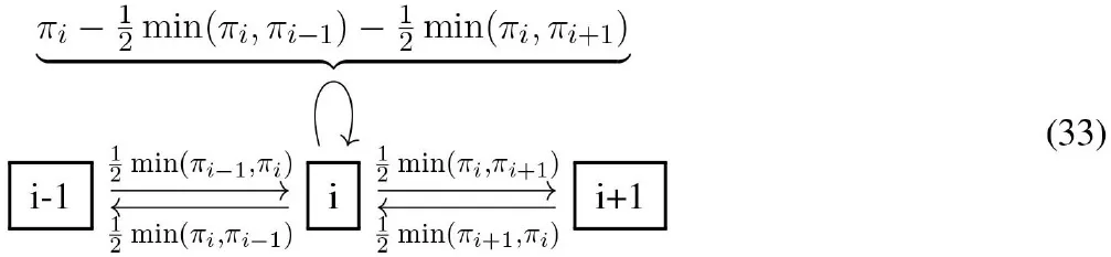
satisfy detailed balance, and the total flow into each configuration i (including from i itself) satisfies the global-balance condition of Equation (2), as already follows from detailed balance.

The displacement-lifted Markov chains in this section, with ${\widehat{\Omega }}_n={\Omega }_n\times \left\{-1,+1\right\}$, split the Metropolis moves i → i ± 1 into two copies (the virtual vertices and edges are also split). The lifted transition matrix is a product of a transport transition matrix ${\widehat{P}}^{\mathrm{\text{trans}}}$ and a resampling transition matrix ${\widehat{P}}^{\mathrm{\text{res}}}$. ${\widehat{P}}^{\mathrm{\text{trans}}}$ describes moves from lifted configuration (i, σ) to (i + σ, σ) that are proposed with probability 1 and accepted with the Metropolis filter min(1, π_i+σ/π_i) given that ${\widehat{\pi }}_{(k,\sigma )}=\frac{1}{2}{\pi }_k\forall k$. Crucially, in the transport transition matrix, if the transport move (i, σ) → (i + σ, σ) is rejected, the lifting move (i, σ) → (i, −σ) takes place instead. ${\widehat{P}}^{\mathrm{\text{trans}}}$ satisfies the global-balance condition for each lifted configuration, as can be checked by inspection:

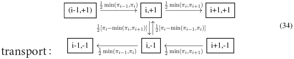
[the flow into (i, σ) equals $\frac{1}{2}{\pi }_i={\widehat{\pi }}_{(i,\sigma )}$].

In the resampling transition matrix, the lifting variable in the configuration (i, σ) is simply switched to (i, −σ) with a small probability ϵ. ${\widehat{P}}^{\mathrm{\text{res}}}$ satisfies detailed balance, and the resampling flows are:

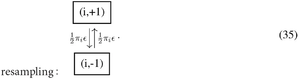
The lifted transition matrix $\widehat{P}={\widehat{P}}^{\mathrm{\text{trans}}}{\widehat{P}}^{\mathrm{\text{res}}}$ satisfies global balance. ${\widehat{P}}^{\mathrm{\text{res}}}$ guarantees aperiodicity of $\widehat{P}$ for any choice of π.

The speedups that can be achieved by lifting on the path graph P_n depend on the choice of π and on the resampling rate ϵ. Bounded stationary distributions are reviewed in subsection 3.1 and unbounded ones in subsection 3.2. All Markov chains on P_n naturally share a diameter bound n, which is independent of π and that (up to a constant) is the same for the lifted chains.

3.1. Bounded One-Dimensional Distributions

In real-world applications of MCMC, many aspects of the stationary distribution π remain unknown. Even the estimation of the maximum-weight (minimum-energy) configuration argmax_{i ∈ Ω}π_i is often a non-trivial computational problem that may itself be treated by simulated annealing, a variant of MCMC [3, 41]. Also, crucial characteristics as the conductance are usually unknown, and the mixing time can at best be inferred from the running simulation. Simplified models, as a particle on a path graph, offer more control. The present subsection reviews MCMC on a path graph for stationary distributions for which $({max}_{i\in {\Omega }_n}{\pi }_i)/({min}_{j\in {\Omega }_n}{\pi }_j)$ remains finite for n → ∞. The conductance bound then scales as $\Phi ~\frac{1}{n}$ as n → ∞, and reversible local MCMC mixes in ${O}(n^2)$ time steps.

3.1.1. Constant Stationary Distribution, Transport-Limited MCMC

For the constant stationary distribution $\pi =\left\{\frac{1}{n},\dots ,\frac{1}{n}\right\}$ on P_n (see [31]), the collapsed Markov chain Π moves with probability $\frac{1}{2}$ to the left and to the right. Rejections take place only at the boundaries i = 1 and i = n and assure aperiodicity. Π performs a diffusive random walk. Its ${O}(n^2)$ mixing time is close to the upper mixing-time bound of Equation (13). As t_mix is on larger time scales than the lower conductance bound, Π is limited by transport.

In the lifted sample space ${\widehat{\Omega }}_n={\Omega }_n\times \left\{-1,+1\right\}$, the transport transition matrix ${\widehat{P}}^{\mathrm{\text{trans}}}$ describes a deterministic rotation on the lifted graph which has the topology of a ring with 2n vertices. ${\widehat{P}}^{\mathrm{\text{trans}}}$ is not aperiodic as its period is 2n (see subsection 2.1.1). Resampling with rate $ϵ=\frac{1}{n}$ with ${\widehat{P}}^{\mathrm{\text{res}}}$ leads to a mixing time of the combined transition matrix ${\widehat{P}}^{\mathrm{\text{trans}}}{\widehat{P}}^{\mathrm{\text{res}}}$ as $t_{\mathrm{\text{mix}}}={O}(n)$ (see [31]).

The resampling, that is, the application of ${\widehat{P}}^{\mathrm{\text{res}}}$, need not take place after each transport step, with a small probability ϵ. One may also resample after a given number ℓ of transport moves, where ℓ may itself have a probability distribution. Such resamplings can also be formulated as Markov chains. In ECMC, resamplings are often required to ensure irreducibility whereas, on the path graph, they merely render the Markov chain aperiodic.

3.1.2. Square-Wave Stationary Distribution

On the path graph P_n with the square-wave stationary distribution ${\pi }_{2k-1}=\frac{2}{3n}$, ${\pi }_{2k}=\frac{4}{3n}\forall k\in \left\{1,\dots ,n/2\right\}$ (for even n), the conductance $\Phi =\frac{2}{3n}$ for n → ∞ is of the same order of magnitude as for the flat distribution. Its bottleneck (the vertex where the conductance is realized) is again at $i=\frac{n}{2}$. The Metropolis algorithm proposes moves from vertex i with probabilities $\frac{1}{2}$ to i ± 1 but rejects them with probability $\frac{1}{2}$ if i is odd (see Equation 16). Its mixing time is ${O}(n^2)$, on the same order as in subsection 3.1.1. The displacement-lifted Metropolis algorithm generates lifting moves with probability $\frac{1}{2}$ on odd-numbered vertices, and the persistence of the lifting variable is lost on finite time scales. In consequence, the displacement lifting is inefficient for the square-wave stationary distribution, with the mixing time still as $t_{\mathrm{\text{mix}}}={O}(n^2)$. More elaborate liftings using height-type lifting variables that decompose $\widehat{\pi }$ into a constant “lane” and another one that only lives on even sites and recover ${O}(n)$ mixing [42].

The success of displacement lifting on the path graph thus crucially depends on the details of the stationary distribution. ECMC in real-world applications is likewise simpler for homogeneous systems with a global translational invariance (or with a similar invariance for spin systems). Remarkably, however, ECMC can apply the same rules to any continuous interparticle potential in homogeneous spaces. It achieves considerable speedups similar to what the lifting of subsection 3.1.1 achieves for the flat stationary distribution on the path graph.

3.2. Unbounded One-Dimensional Stationary Distributions

For unbounded ratios of the stationary distribution (${max}_{ij}({\pi }_i/{\pi }_j)\to \infty$ for n → ∞) the conductance as well as the benefits that can be reaped through lifting vary strongly. Exact results for a V-shaped distribution and for the Curie–Weiss model are reviewed.

3.2.1. V-Shaped Stationary Distribution, Conductance-Limited MCMC

The V-shaped stationary distribution on the path graph P_n of even length n is given by ${\pi }_i=\mathrm{\text{const}}|\frac{n+1}{2}-i|\forall i\in \left\{1,\dots ,n\right\}$, where $\mathrm{\text{const}}=\frac{4}{n^2}$ (see [43]). The stationary distribution π thus decreases linearly from i = 1 to the bottleneck $i=\frac{n}{2}$, with $\pi (\frac{n}{2})=\pi (\frac{n}{2}+1)=\frac{\mathrm{\text{const}}}{2}~n^{-2}$ and then increases linearly from $i=\frac{n}{2}+1$ to i = n. The Metropolis algorithm again proposes a move from vertex i to i ± 1 with probabilities $\frac{1}{2}$ and then accepts them with the filter of Equation (16). The virtual end vertices ensure the correct treatment of boundary conditions. The conductance equals $\Phi =\frac{2}{n^2}$, for the minimal subset $S=\left\{1,\dots ,\frac{n}{2}\right\}$ (see Equation 10). The Metropolis algorithm mixes in S on an ${O}(n^2)$ diffusive timescale, but requires ${O}(n^{2}logn)$ time steps to mix in Ω_n (see [43]). However, even a direct sampling in S, that is, perfect equilibration, samples the boundary vertex n/2 between S and $\overline{S}$ only on a ${\pi }_i/{\pi }_S~n^{-2}$ inverse time scale. For the V-shaped distribution, the benefit of lifting is, thus, at best marginal [from ${O}(n^{2}logn)$ to ${O}(n^2)$], as the collapsed Markov chain is already conductance-limited, up to a logarithmic factor.

The optimal speedup for the V-shaped distribution is indeed realized with ${\widehat{\Omega }}_n={\Omega }_n\times \left\{-1,+1\right\}$, and the transition matrices ${\widehat{P}}^{\mathrm{\text{trans}}}$ and ${\widehat{P}}^{\mathrm{\text{res}}}$. The lifted Markov chain reaches a total variation distance of $\frac{1}{2}$ and mixes in S on an ${O}(n)$ timescale. A total variation distance of $ϵ<\frac{1}{2}$, and mixing in $\widehat{\Omega }$ is reached in ${O}(n^2)$ time steps only [43]. This illustrates that $ϵ<\frac{1}{2}$ is required in the definition of Equation (7).

3.2.2. Curie–Weiss Model, Mixing Times vs. Correlation Times

The Curie–Weiss model (or mean-field Ising model [44]) for N spins s_i = ±1 has the particularity that its total potential

$\begin{array}{ll}U=-\frac{J}{2N}{\displaystyle \sum _{i,j}}{s}_i{s}_j=-\frac{J}{2N}{M}^2,& (36)\end{array}$

with J > 0, only depends on the magnetization $\sum _i{s}_i=M$. The mapping i = (M + N)/2 + 1, n = N + 1, places it on the path graph P_n. The heatbath algorithm (where a single spin is updated) can be interpreted as the updating of the global magnetization state. The model was studied in a number of papers [22, 45–47].

The conductance bound of Equation (10) for the Curie–Weiss model derives from a bottleneck at i = n/2 where U = 0. In the paramagnetic phase, one has $\Phi ={O}(n^{-1/2})$, and at the critical point βJ = 1, $\Phi ={O}(n^{-3/4})$ (see [45]). The corresponding conductance bounds are smaller than n because the magnetization is strongly concentrated around M = 0 (i.e., i = n/2), in the paramagnetic phase. In the ferromagnetic phase, βJ > 1, the magnetizations are concentrated around the positive and negative magnetizations (i ≳ 1 and i ≲ n) and in consequence Φ⁻¹ grows exponentially with n, and so do all mixing times.

The reversible Metropolis algorithm mixes in ${O}(nlogn)$ time steps for T > T_c (see [45]). This saturates the upper bound of Equation (13). At the critical point T = T_c, the mixing time is ${O}(n^{3/2})$. As is evident from the small conductance bound, the Metropolis algorithm is again limited by a slow diffusive transport and not by a bottleneck in the potential landscape.

The displacement lifting of the Metropolis algorithm improves mixing times both for T > T_c and for T = T_c to the optimal ${O}(n)$ scaling allowed by the diameter bound. The correlation time can be shorter than ${O}(n)$ because of the strong concentration of the probability density on a narrow range of magnetizations [22, 46, 47], while the mixing time on the path graph is always subject to the ~ n diameter bound. By contrast, in the paramagnetic phase J > 1, the conductance bound is exponential in n, and all mixing times are limited by the bottleneck at $i=\frac{n}{2}$, that is, the zero-magnetization state.

4. N Particles in One Dimension

The present section reviews MCMC for N hard-sphere particles on a one-dimensional graph with periodic boundary conditions [the path graph P_n with an added edge (n, 1)], and on continuous intervals of length L with and without periodic boundary conditions. In all cases, moves respect the fixed order of particles (x₁ < x₂, …, < x_N−1 < x_N, possibly with periodic boundary conditions in positions and particle indices). With periodic boundary conditions, uniform rotations of configurations are ignored, as they mix very slowly [48]. The hard-sphere MCMC dynamics is essentially independent of the density for the discrete cases (see [49, Equation 2.18]) as well as in the continuum (see [28] and [29, Figure 1]). Most of the hard-sphere results are numerically found to generalize to a class of continuous potentials (see [28, Supplementary Item 5]).

Subsection 4.1 reviews exact mixing and correlation-time results for reversible Markov chains and subsection 4.2 those for non-reversible ones, including the connection with the totally asymmetric simple exclusion process (TASEP). Subsection 4.3 discusses particle-lifted Markov chains, like the PL-TASEP, the lifted-forward Metropolis algorithm as well as ECMC, for which rigorous mixing times were obtained. In many cases, non-reversible liftings including ECMC mix on smaller time scales than their collapsed Markov chains.

4.1. Reversible MCMC in One-Dimensional N-Particle Systems

Although local hard-sphere MCMC was introduced many decades ago [1], its mixing times were obtained rigorously only in recent years, and that too only in one dimension. In the discrete case, the symmetric simple exclusion process (SSEP), the mixing times (and not only their scalings) are known rigorously.

4.1.1. Reversible Discrete One-Dimensional MCMC

The SSEP implements the local hard-sphere Metropolis algorithm in the discrete sample space ${\Omega }^{\mathrm{\text{SSEP}}}=\left\{x_1<x_2<,\dots ,<x_N\right\}$ with x_i ∈ {1, …, n} (periodic boundary conditions understood for positions and indices). All legal hard-sphere configurations c = (x₁, …, x_N) have the same weight ${\pi }_c={\pi }^{*}$, and the displacement set is ${D}=\left\{-1,+1\right\}$. At each time step t, a random element of ${D}$ is applied to a randomly sampled particle i, for a proposed move from c toward one of the 2N neighboring configurations that may, however, not all be legal:

$\begin{array}{ll}\begin{array}{l}{c}_i^{-}=(x_1,\dots ,x_i-1,\dots ,x_N)\\ (-1\text{ move from }c\iff +1\text{ move toward }c)\\ c_i^{+}=(x_1,\dots ,x_i+1,\dots ,x_N)\\ (+1\text{ move from }c\iff -1\text{ move toward }c).\end{array}& (37)\end{array}$

If the sampled configuration is legal, the move is accepted. Otherwise, it is rejected and c remains the configuration for time step t + 1. The algorithm trivially satisfies detailed balance. Global balance follows from a detailed balance for the SSEP, but the validity of Equations (2) and (3) may also be checked explicitly.¹ The total flow into c, which must equal π_c, arrives from the configuration c itself and again from the 2N neighboring configurations of Equation (37) (see [28]): If the configuration $c_i^{-}$ is legal, it contributes forward accepted flow ${{A}}_i^{+}=\frac{1}{2N}{\pi }^{*}$, and ${{A}}_i^{+}=0$ otherwise. If, on the contrary, $c_i^{-}$ is illegal, there is backward rejected flow ${{R}}_i^{-}=\frac{1}{2N}{\pi }^{*}$ from c to c through the rejected backward move $c\to c_i^{-}$. Therefore, ${{A}}_i^{+}+{{R}}_i^{-}=\frac{1}{2N}{\pi }^{*}$, and likewise ${{A}}_i^{-}+{{R}}_i^{+}=\frac{1}{2N}{\pi }^{*}$. The total flow into configuration c is:

$\begin{array}{ll}{\displaystyle \sum _{i=1}^N}({\displaystyle \underset{\frac{1}{2N}{\pi }^{*}}{{\displaystyle \underbrace{{{A}}_i^{+}+{{R}}_i^{-}}}}}+{\displaystyle \underset{\frac{1}{2N}{\pi }^{*}}{{\displaystyle \underbrace{{{A}}_i^{-}+{{R}}_i^{-}}}}})={\pi }^{*}\equiv {\pi }_c,& (38)\end{array}$

so that global balance is satisfied.

The mixing time of the SSEP from the most unfavorable initial distribution π^{0} (the compact configuration) is known to scale as ${O}(N^{3}logN)$, whereas the mixing time from an equilibrium configuration scales only as ${O}(N^3)$, i.e., as the correlation time [49]. These behaviors are recovered by numerical simulation.

4.1.2. Continuous One-Dimensional Reversible MCMC

In the one-dimensional continuum, the scaling for the mixing times of reversible local hard-sphere MCMC has been obtained rigorously for the heatbath algorithm only. In this dynamics, at each time step, the position of a randomly sampled sphere i is updated to a uniform random value in between spheres i − 1 and i + 1. The heatbath algorithm mixes in ${O}(N^{3}logN)$ moves [50] on an interval with fixed boundary conditions. The mixing time for the same model with periodic boundary conditions is between ${O}(N^3)$ and ${O}(N^{3}logN)$ [48]. Numerical simulations suggest ${O}(N^{3}logN)$ mixing on the continuous interval with periodic boundary conditions both for the heatbath and for the Metropolis algorithm [28].

4.2. Non-reversible MCMC in One-Dimensional N-Particle Systems

Non-reversible MCMC in one-dimensional particle systems has a long history in physics and mathematics in the study of the totally asymmetric simple exclusion process (TASEP) [51], which can be interpreted as a displacement lifting of the SSEP. For that model, faster mixing-time scaling than for the SSEP was proven recently. The “particle-lifted” TASEP (PL-TASEP) [28] (with particle lifting on top of the TASEP's displacement lifting) is a lattice version of ECMC. With its chains of particles moving forward and a suitable choice for resampling, it can mix on even faster time scales than the TASEP. Extensions of the hard-sphere case to nearest-neighbor, monotonous potentials with a no-hopping condition were discussed [28, Supplementary Item 5].

4.2.1. Discrete Non-reversible MCMC in One Dimension—TASEP, Particle-Lifted TASEP

The TASEP can be interpreted as a displacement lifting of the SSEP (see subsection 4.1.1) with a displacement-lifted sample space ${\widehat{\Omega }}^{\mathrm{\text{TASEP}}}={\Omega }^{\mathrm{\text{SSEP}}}\times {D}$, with ${D}=\left\{-1,+1\right\}$. Its lifted transport transition matrix randomly proposes a move of sphere i in direction σ, from (c, σ) toward $(c_i^{\sigma },\sigma )$. This move is accepted if $c_i^{\sigma }$ is legal. Otherwise, the system remains at (c, σ) [without performing a lifting move toward (c, −σ)]. A resampling transition matrix could perform such a lifting move on a random particle i. Because of the periodic boundary conditions, the TASEP, for its collapsed configurations, is irreducible and aperiodic even for a vanishing resampling rate ϵ between the elements of ${D}$. One may thus neglect resamplings and retain only one of the elements of ${D}$, say, the +1. The TASEP then simply consists in the +1 half of the SSEP. The effective halving of the lifted sample space for small ϵ carries over, in homogeneous spaces, to higher-dimensional diffusion processes and to ECMC.

The global-balance condition may be checked through the flows into a lifted configuration (c, σ), using the notations of Equation (37).² For the TASEP, the configuration c = (x₁, …, x_N) can evolve into the configurations $c_i^{+}$, as mentioned above. The flows into c now arrive from c itself and possibly from N neighboring configurations $c_i^{-}$ of Equation (37). If the configuration $c_{i-1}^{+}$ is legal, then $c_i^{-}$ contributes accepted flow ${{A}}_i^{+}=\frac{1}{N}{\pi }^{*}$ toward c, and ${{A}}_i^{+}=0$ otherwise. If, on the contrary, $c_{i-1}^{+}$ is illegal, then there is forward rejected flow ${{R}}_{i-1}^{+}=\frac{1}{N}{\pi }^{*}$ from c to c through the rejected forward move $c\to c_{i-1}^{+}$ and ${{R}}_{i-1}^{+}=0$ otherwise. Therefore, ${{A}}_i^{+}+{{R}}_{i-1}^{+}=\frac{1}{N}{c}^{*}$, and the total flow into configuration c is [28]:

$\begin{array}{ll}{\displaystyle \sum _{i=1}^N}({\displaystyle \underset{\frac{1}{N}{\pi }^{*}}{{\displaystyle \underbrace{{{A}}_i^{+}+{{R}}_{i-1}^{+}}}}})={\pi }^{*}\equiv {\pi }_c,& (39)\end{array}$

so that global balance is satisfied (periodic boundary conditions understood).

The TASEP is proven to mix in ${O}(N^{5/2})$ time steps [52], a factor of N^1/2 log N faster than its collapsed Markov chain, the SSEP. The equilibrium correlation time (the inverse gap of the transition matrix that, in this case, can be diagonalized) has the same ${O}(N^{5/2})$ scaling [12, 13]. Numerical simulations (with an operational definition of mixing times [28, Supplementary Item S2]) recover this behavior.

The SSEP allows for particle lifting with respect to the indices ${N}=\left\{1,\dots ,N\right\}$, with the lifted sample space ${\widehat{\Omega }}^{\mathrm{\text{PL-SSEP}}}={\Omega }^{\mathrm{\text{SSEP}}}\times {N}$. Transition matrices, for example, the particle-sweep transition matrices of subsection 2.3.1 then constitute valid liftings of the SSEP, as the latter is a reversible Markov chain with single-particle moves. In contrast, the PL-TASEP, with a lifted sample space

$\begin{array}{ll}{\widehat{\Omega }}^{\text{PL-TASEP}}={\widehat{\Omega }}^{\text{TASEP}}\times {N}={\Omega }^{\text{SSEP}}\times \left\{-1,+1\right\}\times {N},& (40)\end{array}$

is subtle. The particle-sweep transition matrix (with forward moves, and the sample space of Equation 40) violates the global-balance condition because, in essence, ${{A}}_i^{+}$ and ${{R}}_{i-1}^{+}$ add up to a constant in Equation (39), while ${{A}}_i^{+}$ et ${{R}}_i^{+}$ do not. This is not in contradiction with subsection 2.3.1 as the collapsed Markov chain of the particle-sweep (the TASEP) is non-reversible. The PL-TASEP [28], lives in the doubly lifted sample space of Equation (40). Its transport transition matrix advances the lifted configuration (c, σ, i) toward $(c_i^{+},\sigma ,i)$ (see Equation 37) if $c_i^{+}$ is legal. Otherwise, the configuration at time t + 1 is (c, σ, i + 1) (where periodic boundary conditions are understood, sphere i + 1 blocks sphere i). In essence, the PL-TASEP thus consists in repeatedly advancing the same sphere. When such a forward move is rejected, a particle-lifting move results in the sphere causing the rejection to become the new moving sphere.

The transport transition matrix of the PL-TASEP satisfies global balance, and can again be checked by computing the flows into a particle-lifted configuration (c, σ, i). The flows into (c, σ, i) arrive either from (c, σ, i − 1), if $c_i^{-}$ is illegal, or else from $(c_i^{-},\sigma ,i)$, if $c_i^{-}$ is legal. The two flows sum up to a constant. The transport transition matrix of the PL-TASEP is deterministic, and particle resamplings (c, σ, i) → (c, σ, k) with random choices of $k\in {N}$ are required for irreducibility and aperiodicity [28]. Displacement resamplings (c, σ, i) → (c, −σ, i) are not required, and the lifted sample space can again be halved.

With appropriate resamplings, the PL-TASEP mixes on an ${O}(N^{2}logN)$ time scale, much faster than its (doubly) collapsed reversible Markov chain, the SSEP [which features ${O}(N^{2}logN)$ mixing], and even considerably faster than its particle-collapsed non-reversible Markov chain, the TASEP [with ${O}(N^{5/2})$].

4.2.2. Continuous Non-reversible MCMC in One Dimension: Forward, Lifted Forward

The discrete liftings of the SSEP, of subsection 4.2.1, can be generalized to continuous-space liftings of the Metropolis algorithm (with a non-hopping condition) with its collapsed sample space ${\Omega }^{\mathrm{\text{Met}}}=\left\{x_1<x_2,\dots ,<x_N\right\}$ with x_i ∈ [0, L] (periodic boundary conditions understood for positions and indices).³ The displacements ±δ with δ > 0 are proposed from a symmetric distribution that may stretch out to infinity, so that ${D}=ℝ$. The two possible directions in the quotient set ${{D}}_q=\left\{-1,1\right\}$ are used for the displacement lifting. Displacement liftings with respect to the elements of ${D}$ rather than ${{D}}_q$ have not been studied.

The global-balance condition can again be verified for the Metropolis algorithm separately for each δ > 0, with configurations $c_i^{-}(\delta )$ and $c_i^{+}(\delta )$ defined as

$\begin{array}{ll}\begin{array}{c}{c}_i^{-}(\delta )=(x_1,\dots ,x_i-\delta ,\dots ,x_N)(-\delta \text{ move from }c)\\ c_i^{+}(\delta )=(x_1,\dots ,x_i+\delta ,\dots ,x_N)(+\delta \text{ move from }c),\end{array}& (41)\end{array}$

generalizing the 2N neighboring configurations $c_i^{-}$ and $c_i^{+}$ of Equation (37).

The forward Metropolis (“Forward”) algorithm is a displacement lifting of the Metropolis algorithm, with a sample space

$\begin{array}{ll}{\widehat{\Omega }}^{\text{Forw}}={\Omega }^{\text{Met}}\times {{D}}_q\text{(}{{D}}_q\equiv \left\{-1,1\right\}).& (42)\end{array}$

Its lifted transport transition matrix randomly advances sphere i in direction σ by a random step δ on the scale of the mean inter-particle spacing. This advances the configuration from (c, σ) to $(c_i^{\sigma }(\delta ),\sigma$) if the latter is legal. Otherwise the system remains at (c, σ) [without performing a lifting move toward (c, −σ)]. The effective halving of the sample space (to only “forward” moves) carries over from the TASEP. The Forward algorithm is irreducible and aperiodic for appropriate choices of the step-size distribution, and it requires no resampling.

The particle-lifted Forward (PL-Forward) algorithm has a sample space

$\begin{array}{ll}{\widehat{\Omega }}^{\text{PL-Forw}}={\Omega }^{\text{Forw}}\times {N}={\Omega }^{\text{Met}}\times {{D}}_q\times {N}.& (43)\end{array}$

The particle-sweep lifting of the Forward algorithm is again incorrect, as for the TASEP. The transport transition matrix of the PL-Forward algorithm is the continuous-space variant of the PL-TASEP. The same sphere i advances, with random displacements at each time step, until it is blocked by the succeeding sphere i + 1 (periodic boundary conditions understood). In that latter case, a lifting move (c, σ, i) → (c, σ, i + 1) takes place.

The Forward algorithm is numerically found to mix in ${O}(N^{5/2})$ time steps, down from ${O}(N^{3}logN)$ for its collapsed Markov chain (the rigorous results [52] for the TASEP have not been generalized). This reduction is achieved without resampling. The PL-Forward algorithm also mixes in ${O}(N^{5/2})$ time steps, and resampling reduces the mixing-time scaling to ${O}(N^{2}logN)$, as for the PL-TASEP.

4.3. Event-Chain Monte Carlo in One-Dimensional N-Particle Systems

For hard spheres on a one-dimensional line with periodic boundary conditions, ECMC lives in the particle-lifted sample space of the PL-Forward algorithm, itself being a displacement lifting of the Metropolis algorithm (see subsection 4.2.2). It realizes its continuous-time limit, with an infinitesimal expectation of δ_t and a rescaling of time t such that finite times correspond to finite net displacements, usually with a “velocity” equal to one. ECMC is thus a lifting of the Metropolis algorithm with infinitesimal time steps. With the sample-space halving discussed previously, the ECMC lifted transport transition matrix advances the “active” sphere i by infinitesimal δ_t (with all other spheres stationary) until it collides with the succeeding sphere i + 1 (periodic boundary conditions in N understood), at which time sphere i + 1 becomes the sole active sphere. The transport transition matrix of one-dimensional hard-sphere ECMC is thus equivalent to molecular dynamics (the solution of Newton's equations) for an initial condition with a single non-zero velocity +1, and it is purely deterministic.

Particle resamplings assure irreducibility and aperiodicity of the ECMC. It is convenient to have these resamplings take place after each (eponymous) “event chain,” of length ℓ = ∑δ_t, where ℓ can itself have a probability distribution. Such resampling generalize the transition matrix ${\widehat{P}}^{\mathrm{\text{res}}}$ of subsection 3.1. For specific distributions of ℓ, ECMC relaxation can be described exactly. Non-trivial relabelings and factor-field variants illustrate in this exactly solvable case that ECMC is a family of algorithms with different scalings of the mixing times. These times are now to be counted in the number of “events” (i.e., in lifting moves), rather than in the number of infinitesimal moves δ_t. Very generally, ECMC is implemented with a computational effort of ${O}(1)$ per event, and without any discretization in time.

4.3.1. Event-Chain Monte Carlo Stopping Rule, Coupon-Collector Problem

For one-dimensional hard-sphere ECMC, the transport transition matrix is deterministic, and particle resamplings are crucial. The ECMC dynamics of N hard spheres of diameter d on a periodic line of length L is equivalent to the dynamics of N point particles on a reduced line of length L_free = L − Nd. In consequence, one event chain of chain length ℓ effectively advances the sphere that initiates the event chain by ℓ (up to relabeling of spheres). If ℓ is sampled from any uniform distribution in [const, const + L_free], the initial sphere of the event chain is placed (up to a relabeling) at a random position on the ring. ECMC thus obtains a perfect sample when each sphere has once initiated an event chain, allowing the definition of a stopping rule. The solution of the mathematical coupon-collector problem shows that it takes ${O}(NlogN)$ random samples of N possible event-chain starting spheres to touch each of them at least once. In consequence, the number of event chains required for mixing scales as ${O}(NlogN)$, and the total number of events as ${O}(N^{2}logN)$ (see [29, 53].

4.3.2. Event-Chain Monte Carlo With Local Relabeling

The logarithm in the mixing-time scaling ${O}(N^{2}logN)$ of ECMC originates in the coupon-collector probability to repeatedly sample the same starting sphere for different event chains. Naive particle sweeps, however, break the global-balance condition. A correct modified lifted transition incorporates local relabelings as follows: It advances the active sphere i (with all other spheres stationary) until it collides with a sphere j, at which time i and j exchange their labels. The newly relabeled sphere i continues as the sole active sphere. When the event chain terminates (after a continuous time interval ℓ), a new event chain starts with sphere i + 1 as active sphere [29]. With the sweep through active spheres, the coupon-collector-related logarithmic slowdown is avoided so that the choice of random chain lengths ℓ = ran[const, const + L_free], remains as the only random element in the algorithm. It produces a perfect sample after N chains and ${O}(N^2)$ events rather than the ${O}(N^{2}logN)$ events of regular ECMC. ECMC with local relabeling again illustrates that reducing the randomness of moves can speed up mixing, in other words, bring about faster overall randomization. In higher-dimensional hard-sphere systems, the relabeling appears to speed up the approach to equilibrium by only a constant factor [53].

4.3.3. Factor-Field ECMC in One Dimension

The factorized Metropolis filter separates the total potential into independent terms (the factors). Large variations in one factor potential then remain uncompensated by those in other factors, as would be the case for the total potential (for energy-based filters). As a consequence, ECMC may possess event rates that are too high for efficient mixing. This potential shortcoming of standard ECMC was remarked at low temperature in one-dimensional N-particle systems [54] (see also [29, Figure 2]). It is overcome in one-dimensional particle systems through the addition of invariants and their subsequent breakup into factor fields. Such terms may decrease the event rate. Moreover, they can profoundly modify the characteristics of the event-chain dynamics and decrease mixing-time and correlation-time exponents.

For N particles on a one-dimensional interval of length L, the quantity $\sum _i(x_{i+1}-x_i)$ (with periodic boundary conditions in L and in N) is an invariant. A linear function f(x) = ax can transform it into a sum of factor fields:

$\begin{array}{ll}{\displaystyle \underset{\text{invariant}}{{\displaystyle \underbrace{f\left[{\displaystyle \sum _i}(x_{i+1}-x_i)\right]}}}}={\displaystyle \sum _i}{\displaystyle \underset{\text{factor field}}{{\displaystyle \underbrace{f(x_{i+1}-x_i)}}}}& (44)\end{array}$

The factor field of Equation (44) may be added and its linear parameter a adjusted to any pair-factor potential. Attractive factor fields may thus be added to hard-sphere factors or to Lennard-Jones factors [55]. With the linear factor adjusted to compensate the virial pressure, ${O}(N^{3/2})$ autocorrelation times [rather than ${O}(N^2)$ without factor fields] and ${O}(N^2)$ mixing times [rather than ${O}(N^{2}logN)$] are found. One particular feature of event-chain dynamics at the optimal value of the factor field is that the chains have zero linear drift, and therefore also vanishing virial pressure [8, 55].

5. Statistical-Mechanics Models in More Than One Dimension

The present section reviews ECMC for statistical-physics models in more than one dimension. At a difference with the lifted Markov chains considered in section 4, the displacement of an active particle impacts several factors, and the next veto arises from one of them (an active particle may, for example, collide with one out of several other particles and form separate factors with each of them). Subsection 5.1 reviews mathematical and algorithmic aspects of the two-dimensional (2D) hard-disk model, the first application of ECMC [5, 7, 56] where vetoes are determined deterministically. Hard-disk ECMC is contrasted with related algorithms that were applied to this system. Subsection 5.2 reviews ECMC for the harmonic model of a solid, but which is also the low-temperature effective model for continuous-spin systems, as the XY or the Heisenberg models. In these spin systems, as in the harmonic model, ECMC can be thoroughly analyzed. Subsection 5.3 reviews the interplay between spin waves and topological excitations for local Markov chains including ECMC, whose behavior there is much better understood than for particle systems.

5.1. Two-Dimensional Hard Disks

Hard-sphere ECMC can be analyzed without reference to the factorized Metropolis algorithm, as is necessary for more general interactions. Most studies have concentrated on the 2D case, the hard-disk model, whose phase behavior was clarified using ECMC [5, 57] after decades of uncertainty (The original Fortran90 implementation used in [5] is publicly available [58]). Strictly speaking, hard-disk ECMC is not generally irreducible in the NVT ensemble of fixed volume and number of disks, because of the existence of locally stable configurations at arbitrarily small density in the thermodynamic limit [59]. Such configurations can be formally excluded, and irreducibility established, in the NPT ensemble of constant pressure, although the locally stable configurations are too rare to play a role for a large number of disks N. Hard-disk ECMC is found to be very fast, but elementary questions as, for example, the scaling of correlation times with system size are still without even a clear empirical answer in the ordered phases. The simplifications related to the existence of a constraint graph of possible lifting moves have enabled a successful implementation of hard-disk multithreaded ECMC [58].

5.1.1. Characterization of Hard-Disk ECMC

Hard-disk ECMC lives in a lifted sample space

$\begin{array}{ll}{\widehat{\Omega }}^{\text{ECMC}}={\Omega }^{\text{Met}}\times {{D}}_q\times {N},& (45)\end{array}$

where Ω^Met is the sample space of the Metropolis algorithm (the configuration space of N hard disks, say, in a square box with periodic boundary conditions), ${{D}}_q$ is the quotient set of the displacements (see subsection 2.3.2), and ${N}$ the set of particle indices. For the “straight” ECMC [7] used in all large-scale simulations, ${{D}}_q=\left\{(\pm 1,0),(0,\pm 1)\right\}$. The halving of the homogeneous lifted sample space (see subsection 4.2.1) again allows one to restrict displacements to the positive x and the positive y directions, but this applies to homogeneous hard-disk systems only. The lifted transport transition matrix of straight hard-sphere ECMC advances the active disk i until it collides with another disk j, at which time a particle-lifting move takes place, and j becomes the active disk. This effectively one-dimensional process is equivalent to the one described in subsection 4.3. Particle and displacement resamplings assure irreducibility of straight ECMC (with the above-mentioned caveat related to locally stable configurations). Placed at the beginning of each event chain, they may select the chain's random starting disk and overall direction. The correctness of straight ECMC follows from the continuum limit of a hard-disk lattice version as well as from a mapping onto molecular dynamics with 2D sphere positions but with one-dimensional sphere velocities (see [58, Lemma 1]). A variant of straight ECMC with a larger quotient space ${{D}}_q$ and a transition matrix that slowly changes directions was found to bring no improvements for hard disks [60], while it has drastic effects for hard-sphere objects with internal degrees of freedom [32].

The “reflected” ECMC is also compatible with the necessary conservation of phase-space volume [7]. Its quotient set is ${{D}}_q=\left\{{\widehat{\text{e}}}_{\varphi }:\varphi \in [0,2\pi )\right\}$, where ${\widehat{\text{e}}}_{\varphi }$ is the 2D unit vector in direction ϕ. The lifted transport transition matrix of reflected ECMC only differs in the particle-lifting moves at a collision between a disk i and disk j. To define the outgoing direction, the incoming one is reflected with respect to the line (hyperplane) of incidence (see [56, Figure 2.8]). Reflected ECMC is irreducible without resamplings. Resampling also seem to have little influence on convergence times. In hard-disk applications, however, straight ECMC is generally faster [7, Figure 6]. Variants of the reflected ECMC algorithm, such as the “obtuse reflected” and the Newtonian ECMC [61], appear to be very fast in 3D hard spheres.

In hard-disk and hard-sphere systems, the computation of the pressure is notoriously complicated, as the virial cannot be extracted from a finite number of equiprobable configurations. Instead, it is obtained from an extrapolation of the pair-correlation function to contact [56, section 3.3.4]. In ECMC, the infinite number of highly correlated samples between any two lifting moves allows for an estimator of the virial pressure from the expectations of basic geometrical properties of the ECMC trajectory [8, 57, 62]. This estimator generalizes from hard spheres to arbitrary potentials.

In (straight) ECMC of monodisperse disk, any particle-lifting move (at a collision) can only go from a disk i to a set of at most three other disks, that remains fixed between direction liftings.⁴ An oriented constraint graph, with at most three outgoing arrows for every disk, encodes these relations [63]. The constraint-graph formulation of hard-sphere ECMC exposes its close connection with the harmonic model where subsection 5.2, where the neighbor relations are fixed permanently.

In 2D hard-disk MCMC algorithm, the total variation distance or spectral gaps cannot be estimated or evaluated, and theoretical bounds cannot be used [64]. Rigorous mixing-time scaling exponents are available for low density, but only for a non-local version of the Metropolis algorithm [65]. The analysis of all recent computations builds on the hypothesis that for 2D disks the autocorrelation function of the global orientational order parameter is the slowest relaxation process in this system. Practical computations generally adopt a square box with periodic boundary conditions, where the expectation of the above autocorrelation function vanishes because of symmetry, simplifying the interpretation of time series [5, 7].

5.1.2. Hard-Disk ECMC and Other Algorithms

In general ECMC, the continuous-time limit serves only to associate each veto in the factorized Metropolis algorithm with a unique factor. In the simpler setting of hard-disk ECMC, the continuous-time limit makes that an active disk i only collides with a single other disk j, so that the lifting move i → j is well-defined and compatible with global balance. For two hard disks in a box with periodic boundary conditions, ECMC needs only a single factor, so that the continuous-time limit is not needed. ECMC satisfies the global balance with finite displacements ${D}=\left\{(\pm {\delta }_x,0),(0,\pm {\delta }_y)\right\}$. Because of homogeneity, a given event chain, say, with a fixed displacement (δ_x, 0) then maps to the displacement-lifted transport transition matrix ${\widehat{P}}^{\mathrm{\text{trans}}}$ on a path graph (see subsection 3.1.1), with the displacement of one hard disk corresponding to the “+1” sector on the path graph, and the displacement of the other corresponding to the “−1” sector.

For any N and any spatial dimension D, the transport transition matrix of straight hard-sphere ECMC is equivalent to modified molecular dynamics with D-dimensional positions, yet one-dimensional velocities. This corresponds to hard spheres on one-dimensional constraining “rails” that remain fixed in between direction liftings. The ECMC events correspond to molecular-dynamics collisions, which conserve energy and momenta for a phase-space configuration with only a single non-zero velocity.

A discrete-time precursor algorithm of hard-disk ECMC [66, section 5] also moves chains of disks. For each chain, it samples a random initial disk and a random direction ${\widehat{\text{e}}}_{\varphi }$ of displacement (such that ${\widehat{\text{e}}}_{\varphi }$ and its inverse ${\widehat{\text{e}}}_{\varphi +\pi }$ are equally likely), and a total number n_c of disks to be displaced. A chain move is then constructed (not unlike ECMC) by displacing n_c − 1 disks (starting with the initial one) along the direction of displacement until they hit their successor disks. The (final) disk n_c is placed randomly between its initial position and its (hypothetical) event position with a successor disk. In order to satisfy detailed balance, this algorithm requires a Metropolis rejection step for the entire chain by the ratio of the intervals available for the first and for the final disks. One chain of the precursor algorithm resembles the transport stage of ECMC between particle resamplings, although it can neither be interpreted as a continuous-time Markov chain nor as a lifting. The convergence properties of this algorithm have not been analyzed.

5.1.3. Parallel Hard-Disk ECMC

The hard-disk model was successfully simulated in parallel using domain decomposition, overcoming some of the problems of such a scheme in molecular dynamics [67]. Within ECMC [63, 68], domain decomposition leads to residual interactions that destroy space homogeneity and therefore the convenient halving of the sample space. Convergence is then slower. Within a four-color checkerboard scheme, a cell of any one color touches only differently colored cells [57, 69]. At any time, disks in cells of one given color can thus be updated in parallel. Irreducibility is assured by frequently translating the four-color checkerboard by a random vector. With the collapsed Metropolis algorithm as a sampling algorithm inside cells, this algorithm overcomes its considerable speed handicap (roughly, two orders of magnitude in single-processor mode), through massive parallelization on GPUs. Massively parallel MCMC has been tested to high precision against ECMC and against event-driven molecular dynamics for the pressure and the orientational and positional order parameters [57]. Related work was performed with ECMC replacing the Metropolis algorithm inside each cell [68].

Hard-disk ECMC remains valid for more than one active particle [58], and it then resembles event-driven molecular dynamics, albeit with a much smaller number of moving particles. In single-processor mode, both identify the earliest one of a number of candidate events, the one that will be realized as an event and lead to a lifting move (for ECMC) or to a collision (for molecular dynamics). In both approaches, the event then generates new candidate events, while some of the old ones continue to exist and yet others disappear.

Modern event-driven molecular dynamics codes optimize the management of a very large number of such candidate events [70, 71]. In event-driven molecular dynamics, an extensive number ∝N of candidate events are present at any given moment. The possible scheduling conflicts among this large number of candidate events has long stymied attempts to parallelize the algorithm and to handle several events independently from each other [72–76]. In ECMC, one may freely choose the number of active particles and keep it fixed throughout a simulation. If this number is $\lesssim \sqrt{N}$, the mathematical birthday problem shows that the candidate events are usually disjoint for any two active particles, cutting down on the degree of interference. A framework of local times has lead to a multithreaded implementation for hard-disk ECMC in which scheduling conflicts appear with small finite probability for $~\sqrt{N}$ active disks in the N → ∞ limit for finite run times [58].

5.2. Harmonic Model

The harmonic model [77] describes spin-wave excitations for N spins on a lattice, with a total potential $U=\frac{1}{2}\sum _{\langle i,j\rangle }{({\varphi }_i-{\varphi }_j)}^2$ between neighbors 〈i, j〉, with non-periodic angles ϕ_i ∈ ℝ, which approximate the small elongations |ϕ − ϕ_j| ≪ 1 in the XY model with its total potential $U=-\sum _{\langle i,j\rangle }cos({\varphi }_i-{\varphi }_j)$. Spin waves are the dominant excitations in the XY model at low temperatures, notably in two dimensions [78]. The harmonic model also provides the quintessence of phonon excitations in particle systems, for small displacements from perfect lattice positions. In the harmonic particle model, each particle interacts with a fixed set of neighbors so that disclinations, dislocations, and stacking faults cannot develop.

Besides its role of isolating phonon and spin-wave excitations of many systems, the harmonic model is of importance for hard-sphere ECMC whose sequence of constraint graphs [58, 63], between displacement resamplings, effectively defines a sequence of models with fixed neighborhoods.

5.2.1. Physics of the Harmonic Model

The harmonic model is exactly solved [77]. It has a single phase for all finite temperatures, but the nature of this phase depends on the spatial dimension D. The differences in angle for two spins at positions distant by r for the harmonic spin model (and similarly the difference in elongations with respect to the lattice positions for the harmonic particle model) in equilibrium are given by:

$\begin{array}{ll}{\displaystyle \underset{\text{spin harm.}}{{\displaystyle \underbrace{\langle {(\Delta \varphi )}^2\rangle }}}}~{\displaystyle \underset{\text{part. harm.}}{{\displaystyle \underbrace{\langle {(\Delta \text{r})}^2\rangle }}}}\propto \{\begin{array}{ll}r& \text{for dimension }D=1\\ logr& \text{for }D=2\\ \text{const}& \text{for }D\ge 3.\end{array}& (46)\end{array}$

For a system of size L, the mismatch of two typical spins or particles is thus of the order of ${O}(\sqrt{L})$ in one dimension, grows as the square root of the logarithm of L in two dimensions, and remains constant in three dimensions and higher. The harmonic particle model, in two dimensions, features long-range orientational order but only power-law decay of positional order [79]. Only in more than two dimensions does it have long-range orientational and positional order.

5.2.2. ECMC Algorithm for the Harmonic Model

For the harmonic spin model, the ECMC takes place in a particle and displacement-lifted sample space ${\Omega }^{\mathrm{\text{harm}}}\times {{D}}_q\times {N}$ where ${\Omega }^{\mathrm{\text{harm}}}=\left\{{\varphi }_i\in ℝ:\forall i\right\}$ is the sample space of N generalized angles (although only differences of angles are important), where the periodicity of angles is abandoned. ${{D}}_q=\left\{-1,1\right\}$ is again the quotient set of (infinitesimal) displacements. The homogeneity in ϕ_i again allows the lifted sample space to be halved and the positive direction of displacement to be retained only. ECMC monotonically increases each of the ϕ_i, at a difference of Metropolis MCMC, which must allow for changes of the angles in both directions. In event-driven harmonic-model ECMC, for a finite number of neighbors per spin, the displacement per event of each active spin is finite. It can be expected that the total displacement of each spin or particle corresponding to the Δϕ or Δr in Equation (46) decorrelates the system. It thus follows that from one independent sample to the next one each particle or spin must be displaced ${O}(\sqrt{L})$ times in one dimension, ${O}(\sqrt{logL})$ times in two dimensions, and a constant number of times in more than two dimensions. Reversible local MCMC, in contrast, requires ∝ L² displacements per spin (or particle) for all dimensions. This translates into ECMC correlation times of ${O}(N^{3/2})$, ${O}(N\sqrt{logN})$ and ${O}(N)$ single events, in dimensions D = 1, 2, and 3. Numerical simulations are in excellent agreement with these expectations [80, Figure 7].

5.3. Event-Chain Monte Carlo for Continuous Spin Models

Event-Chain Monte Carlo readily applies to XY and Heisenberg-type spin models because their spin–spin pair potentials on neighboring sites i and j write as U(ϕ_i − ϕ_j) with continuous spin angles ϕ_i and ϕ_j. The particle and direction-lifted sample space for these models is analogous to that of the harmonic model, but with angular variables ϕ ∈ [0, 2π) (the spins of the Heisenberg model must be projected onto a plane in spin space). The homogeneity of the potential with respect to the absolute spin angles again allows the halving of lifted sample space. The particle and direction-lifted transition matrix rotates a given spin i in one direction until the factorized Metropolis algorithm calls for a veto by a neighbor j of i followed by a lifting move from i to j. The spin j then starts to rotate in the same sense, with the cumulative rotation corresponding to the MCMC time.

In the XY model, the 2D fixed-length continuous spins live on a D-dimensional spatial lattice. The pair potential U_ij = −cos(ϕ_i − ϕ_j) favors the alignment of neighboring spins i and j, and in ECMC, the activity (i.e., the rotation) passes from one spin to one of its neighbors. XY-model ECMC is irreducible without any resamplings. Its sequence of active spins realizes an anomalous 2D diffusion process [81]. ECMC on the Heisenberg model, where spins are 3D, can be reduced to this case, with resamplings through rotations in 2D sub-planes in spin space. In both models, ECMC lowers the scaling of relaxation times with respect to local reversible MCMC. Although more efficient algorithms are available [82–84] for these particular models, the comparison of ECMC with reversible MCMC illustrates what can be achieved through non-reversible local Markov chains in real-world applications.

In the 2D XY model, ECMC autocorrelation functions can be fully explained in terms of spin waves and topological excitations. The 2D hard-disk system similarly features phonons and two types of topological excitations, but the precise relaxation dynamics of MCMC algorithms has yet to be clarified (for a synopsis, see [56, Chapter 1]).

5.3.1. Spin Waves and Topological Excitations in the 2D XY Model

Although it possesses no long-range spin order at finite temperatures, the 2D XY model famously undergoes a phase transition [82, 85] between a low-temperature phase rigorously described by spin waves with bound vortex–antivortex pairs [77, 78], and a high-temperature phase where these topological excitations are free.

In the low-temperature phase, vortices pair up with antivortices. The maximum d_max of all vortex–antivortex pair separations in a system of size L × L follows a Fréchet distribution [80],

$\begin{array}{ll}\mathbb{P}\left(d_{max}\right)=\frac{\alpha }{s}{\left(\frac{d_{max}}{s}\right)}^{-1-\alpha }exp\left[-{\left(\frac{d_{max}}{s}\right)}^{-\alpha }\right],& (47)\end{array}$

with a size-dependent scale $s=L^{2/\alpha }{s}_0$ and a size-independent exponent α that depends on the inverse temperature β. Throughout the low-temperature phase, $d_{max}~L^{2/\alpha }$, with α > 2 increases slower than the system size L for non-zero temperatures. Only in the zero-temperature limit does d_max remain constant as the system size increases (α → ∞ for T → 0). It is extensive as the transition point is approached (d_max ~ L, that is, α → 2 for T → T_c).

5.3.2. Relaxation Time Scales in Spin Models

In spin models, MCMC simulations must relax spin waves and topological excitations. In the two-dimensional XY model of length L, reversible energy-based MCMC can be expected to diffusively relax spin waves on an ${O}(L^2)$ time scale at all temperatures [80] and topological excitations on an ${O}(d_{max}^2)$ time scale, so that the overall correlation time scales as ${O}(L^2)$ from both contributions. ECMC relaxes spin waves on a much faster time scale that, from the analogy with the harmonic model, can be thought to be ${O}(logL)$, leading to very fast (system-size-independent) initial decay of spin–spin autocorrelations. The diffusive relaxation of topological excitations by ECMC on the ${O}(d_{max})={O}(L^{4/\alpha })$ time scale is dominant at large times throughout the low-temperature phase, with the two contributions leading to a two-timescale decay of spin autocorrelations [86, 87]. The above arguments are borne out by numerical computations [80] with the α of Equation (47) as the single non-trivial parameter.

6. ECMC and Molecular Simulation

In molecular simulation of classical atomic models with explicit solvents, sampling plays a complementary role [88] to the study of explicit time dependence. However, the complexity of total potentials only allows for Markov chains with local moves. Intricate a priori probabilities or cluster MCMC algorithms [89, 90] have not met with success. The Metropolis or the heatbath algorithms are energy-based. The required evaluation of the Coulomb potential then leads to a prohibitive time consumption for MCMC. In the field, molecular dynamics codes are therefore used exclusively. Great effort has been directed toward the computation of the forces (the derivatives of the total potential), which remains onerous and not entirely approximation-free. Molecular dynamics invariably implements the Newtonian relaxation dynamics. Molecular-dynamics codes developed over the last three decades (e.g., [91]) have found scores of real-world applications from biology to medicine, physics, and chemistry. Molecular dynamics is thus highly successful, but it leaves little algorithmic freedom.

ECMC may represent a new starting point for the use of MCMC for real-world applications in molecular simulation and other fields. First, to sample the Boltzmann distribution π ∝ exp(−βU) without approximations, the potential U (and in particular the Coulomb potential) need not be evaluated. Second, different factorizations and liftings constitute families of inequivalent Markov chains with different scalings of the mixing times. Subsection 6.1 reviews the theoretical aspects of ECMC in the context of molecular simulation while subsection 6.2 provides an overview of the “JeLLyFysh” Python application,⁵ an open-source ECMC implementation for molecular simulation.

6.1. Theoretical Aspects of ECMC for All-Atom Models

Three main challenges stand out for the application of ECMC to molecular simulation. First is the choice of the statistically independent factors, which determines total event rates, as well as mixing and correlation times (see subsection 6.1.1). The second challenge for ECMC, reviewed in subsection 6.1.2, is the handling of the Coulomb potential. The statistical independence of factors obviates the need for evaluating the total potential. However, the factor potential and its derivatives (which yields the event rates) must be provided. One such factor may consist of a single pair of charges together with all their periodic images (“merged-image” Coulomb factor) or else of one pair of specific periodic image charges (“separate-image” Coulomb factor). Both choices are practical, with the latter featuring an infinite number of factors already for a two-charge system in a periodic box [21, 36]. A single merged-image or separate-image Coulomb dipole factor may collect all the electrostatic potentials between all atoms of two molecules. At large separation, the event rate of a dipole factor decreases on a faster scale than for a collection of atomic pair factors. Finally, the choice of the lifting variables ${L}$ in $\widehat{\Omega }=\Omega \times {L}$, as well as the lifted transition matrices appear as main fixtures in a largely uncharted territory. As reviewed in subsection 6.1.3, a lifting move⁶ is uniquely determined only for factors with few elements. For larger factors, the lifting move must itself be sampled from a probability distribution, or even from a choice of many distributions, so-called lifting-move schemes [33]. Different lifting-move schemes can lead to radically different MCMC trajectories for an identical choice of lifted sample spaces and factors [21]. The influence of the choice of lifting variables (for example, the choice of directions, individual moves, etc.) on the mixing properties remains poorly understood (see subsection 6.1.3).

6.1.1. Factors, Coulomb Factors

The Coulomb problem illustrates the algorithmic inequivalence of different factorizations. With Coulomb pair factors between each individual pair of charges distant by r (both for merged-image or separate-image formulations) the pair-factor potential is ~ 1/r, and the pair-factor event rate ~ 1/r². In a 3D box of side L, at fixed density, so that N ∝ L³, a typical event rate between two charges is ~ 1/L² and the total event rate for Coulomb pair factors is ${O}(N/L^2)={O}(N^{1/3})$[36] (see also [21, Equation 89]). With this rate, one event corresponds to a single particle moving forward by ${O}(1/N^{1/3})$. To advance N charges by a constant displacement (for example, 1 Å), Coulomb pair factors require a computing effort of ${O}(N^{4/3})$. This is clearly borne out by numerical simulations (see [36] for details).

For a Coulomb dipole factor made up of all the atoms in two charge-neutral molecules with finite dipole moments, the active particle in one of the molecules effectively interacts with a dipole in the other molecule. At a distance r between molecules, this gives a factor potential ~ 1/r² and a factor event rate ~ 1/r³. Integrated over 3D space in a box of sides L, the total event rate scales as ${O}(logN)$. Advancing N charges by a constant distance requires in this case ${O}(NlogN)$ events, as was observed in N-body simulations [21, Figure 13].

In real-world applications, such as the SPC/Fw water model [92], the interparticle potential contains, beyond the Coulomb term, bond-fluctuation, bending, and Lennard-Jones contributions. For large N, the ${O}(NlogN)$ Coulomb event rate dominates the local contributions, as was observed in simulations (see [21, Figure 15]). In ECMC, it can be expected that the Coulomb dipole factors have mixing and correlation times that are a factor of N^1/3/log N smaller than those for Coulomb atomic factors, although this has not been verified explicitly.

6.1.2. Computation of Coulomb Event Rates

The evaluation of the Coulomb potential and of its derivatives is the main computational bottleneck for molecular simulation. Molecular dynamics simultaneously requires the derivatives of the full Coulomb potential for all particles at each time step. The dominant Ewald-sum-based solution of this problem consists in discretizing charges onto a fine spatial lattice and in solving Poisson's equation using fast Fourier transformation. The complexity of this algorithm is ${O}(NlogN)$ with a pre-factor that increases with the numerical precision (see [6] and [21, section 1A]) The difficulty in evaluating the difference of the Coulomb potential also frustrates energy-based local-move MCMC: Updating a single particle costs at least ${O}(N^{1/2})$ with known algorithms [93], so that a sweep of local moves costs a prohibitive ${O}(N^{3/2})$.

Event-Chain Monte Carlo only computes the veto among the ${O}(N)$ Coulomb factors as well as the ensuing lifting move. A naive implementation of the factorized Metropolis algorithm samples all candidate events (one for each Coulomb factor involving the active particle) to determine the earliest one. The thinning implemented in the cell-veto algorithm reduces the complexity of this computation from ${O}(N)$ to ${O}(1)$, because in a first step, the position-dependent Coulomb factor event rates are “thickened” into time-independent, pre-computed rates, from with a provisional event is computed using the Walker's algorithm. Specific computations are required only in a second step, to confirm the provisional veto.

The separate-image and the merged-image formulations of ECMC both lead to conditionally converging sums that can be regularized in a way that is compatible with traditional approaches. In the separated-image formulation of the Coulomb problem, counter-line-charges [36] and their generalizations, for example, the counter-volume-charges [21, Figure 5], regularize each individual image charge. Likewise, in the merged-image formulation, the sum over all images with associated compensating line charges is equivalent to the standard tin-foil boundary condition [94] for a single pair of Coulomb charges in a finite periodic box (see [21, section III]).

6.1.3. Event-Chain Monte Carlo Liftings and Lifting-Move Schemes for Molecular Simulation

As emphasized throughout this review, the factorized Metropolis algorithm attributes each MCMC rejection to a single factor and transforms it, in ECMC, into a lifting move. For a pair factor, this lifting move is usually determined uniquely (the active and the target particles exchange roles). For a three-particle factor, the probability distribution for the new active particle is uniquely determined, whereas for larger factors, there is a choice among probability distributions, so-called “lifting-move schemes.” For Coulomb dipole factors of two water molecules, each such factor contains six particles, and lifting-move schemes can differ in their inside-flow (active particles on the same molecule for the in-state as for the out-state) and in their outside-flow. This is exemplified in the “inside-first” and the “outside-first” lifting-move schemes [21].

For a factor in which the two molecules are separated by a distance r, the intra-molecular lifting-move rate scales as 1/r³ for the inside-first lifting scheme whereas the lifting-move rate toward the other molecule scales as 1/r⁴. Integrated over the whole simulation box of length L, the (unnormalized) probability that a lifting move remains within one molecule scales as log L, whereas the probability that a lifting move goes from one molecule to another remains constant. For large L, the lifting moves thus remain inside the original molecule with probability 1. For the outside-first lifting-move scheme, in contrast, both the intra-molecule and the inter-molecule rates are ~ 1/r³ as a function of the distance between molecules, and the probabilities for lifting moves to stay inside one molecule or to connect different molecules both scale as ~ log L for large L [21, Table 1].

6.2. JeLLyFysh Application for ECMC

The open-source “JeLLyFysh” application [38] is the first general-purpose open-source implementation of ECMC. The configuration files of its Version 1.0 realize proof-of-concept of ECMC for interacting particle systems including the treatment of the Coulomb interaction. They also showcase different factorizations and lifting-move schemes as well as thinning strategies through bounding potentials and through the cell-veto algorithm. The application strives to provide a platform for future method development, for benchmarking and for production code. The architecture of the application (using the mediator design pattern) mirrors the mathematical structure of ECMC. Its event-driven nature is far removed from the time-driven setup of present-day molecular dynamics codes.

6.2.1. Mediators, Activators, and Event Handlers

The “JeLLyFysh” architecture is entirely based on the concept of events. A mediator [95] serves as a central hub for all other elements of the code. After each event, the mediator accesses the active particles (in fact, the “active global state”) and then fetches from another element, the activator, so-called event handlers that each treat one factor (depending on the active particle but also on the previous event). For each event handlers (i.e., roughly, for each factor), the mediator then accesses the in-state for each factor, which allows the event handler to compute a candidate event time. All candidate event times are compared in an element of the program called a scheduler. For the shortest time in this scheduler, the corresponding event handler then computes the lifting event in the form of an event out-state. If confirmed, the out-state is committed to the state of the system. Output may also be generated (see [38, Figure 5]).

Besides the events (in other words, the lifting moves) required by the global-balance condition, the JeLLyFysh application implements a number of pseudo-events, that handle data and cell management, resamplings, and even for the start and the end of the program. The application makes full use of the fundamental modularity of ECMC. For example, each event handler, for a factor M, only receives the factor in-state c_M in Equation (14) in order to contribute a candidate event. It computes the out-state of M only if this factor actually triggers the veto, that is, generates the lifting move.

6.2.2. Configuration Files, Performance Tests

The configuration files of JeLLyFysh Version 1.0 construct runs for two charged point masses, for interacting charged dipoles, and for two interacting SPC/Fw water molecules, each with a large choice of factors, and high-precision comparison with reversible MCMC. Four different configuration files treat two interacting SPC/Fw water molecules, with their harmonic oxygen–hydrogen bond interaction on one molecule, a three-body bending potential, a Lennard-Jones oxygen–oxygen potential as well as a Coulomb potential between atoms on different molecules [21, Figure 12]. The configuration files illustrate the possibilities offered to choose between atomic and molecular factors, and to implement event-handlers that invert potentials to obtain direct event rates, to use bounding potentials, or even to invoke the cell-veto algorithm. Correlation functions are shown to agree in the 0.1% range.

Performance tests of ECMC for large systems of SPC/Fw water molecules will be the object of the next version of the JeLLyFysh application. It will feature substantially rewritten code, and many of the Python modules will be making use of a faster compiled language. Benchmarks will be provided against single-processor LAMMPS code.

7. Prospects

This review has addressed the mathematical and algorithmic foundations of non-reversible Markov chains including ECMC and analyzed a number of exactly solved test cases. It has also discussed first applications of ECMC to key models in statistical physics as well as an ongoing initiative to apply it in the field of molecular simulation. It is now time to summarize the principal characteristics of ECMC, to formulate the main working assumptions driving its development, and to attempt to anticipate its major challenges.

Event-Chain Monte Carlo reinterprets three key aspects of standard MCMC. First, as in all non-reversible Markov chains, the detailed-balance condition is replaced by global balance. The condition of vanishing flows, synonymous to the notion of “equilibrium,” is thus replaced by a steady-state condition, with the hope of accelerating transport throughout sample space. Second, the energy-driven Metropolis algorithm is replaced by the factorized Metropolis algorithm: as long as a certain consensus condition is satisfied by all factors, the ECMC dynamics is that of a non-interacting system. Third, each of the trademark rejections of the Metropolis algorithm is replaced by a veto of a single factor that puts an end to the consensus and generates a lifting move.

The ongoing development of ECMC for molecular simulation and related fields builds on two assumptions. The first assumption is that Newtonian dynamics, while being physically realistic, is not the fastest possible relaxation algorithm toward the stationary distribution. The three-decade-long investment in molecular-dynamics codes may thus leave room for successful alternative approaches. The second assumption is that the elaborate a priori choices, as in the cluster algorithms, cannot be adapted to real-world applications in molecular simulation and related fields, given their intricacy. This leaves one with local-move Markov chains but, as argued throughout this review, they must be non-reversible in order to be fast. The family of ECMC algorithms provides a framework for non-reversible local MCMC. It opens up numerous opportunities, from the choice of factors and liftings to the new approach to the Coulomb problem that avoids the computation of the potential and its derivatives.

Event-Chain Monte Carlo enlarges the possibilities of the MCMC algorithm and has already found successful specific applications in statistical physics, as well as in polymer science [96, 97] (see also the related review [98]). As a general method for molecular simulation, ECMC however faces two critical short-term challenges. The first concerns the benchmarks against molecular dynamics for standard real-world systems, that will be the object of an upcoming version of the JeLLyFysh application. The second challenge concerns the parallelization of ECMC. A road-map for multithreaded ECMC exists at present only for hard-sphere systems. The development of genuine parallel event-driven ECMC for generic potentials constitutes an open research subject. More generally, the mathematical understanding of the mixing and relaxation dynamics of reversible and non-reversible local MCMC remains rudimentary for generic N-particle models in more than one dimension. A better mathematical grasp of such systems, beyond straightforward benchmarks, appears as a prerequisite for the development of faster algorithms for applications in physics and other sciences.

Author Contributions

The author confirms being the sole contributor of this work and has approved it for publication.

Funding

The author acknowledges support from the Alexander von Humboldt Foundation.

Conflict of Interest

The author declares that the research was conducted in the absence of any commercial or financial relationships that could be construed as a potential conflict of interest.

Acknowledgments

The author was indebted to S. C. Kapfer for extensive discussions on section 3, to S. Todo for numerous discussions on section 2.2.2, and to P. Diaconis, T. A. Kampmann, B. Li, and M. Weber for critical readings, comments, and suggestions.

Footnotes

1. ^This prepares for the analysis of the lifted Markov chains of subsection 4.2.

2. ^The lifting index σ for configurations (c, σ) is dropped for the TASEP, as only the +1 element of ${D}$ is considered.

3. ^In one dimension, configurations and Metropolis algorithm are independent of density.

4. ^This generalizes from the TASEP and the Forward algorithm of subsection 4.1, where the order between spheres remains unchanged because of the no-hopping condition so that lifting moves are always from sphere i to sphere 1+1.

5. ^The name echoes creatures which, like objects studied in molecular simulation, mostly contain water, with some other elements, including proteins.

6. ^As the lifting move (i, σ) → (i, −σ) for a rejected transport move (i, σ) → (i + σ, σ) on the path graph of section 3.

References

1. Metropolis N, Rosenbluth AW, Rosenbluth MN, Teller AH, Teller E. Equation of state calculations by fast computing machines. J Chem Phys. (1953) 21:1087–92. doi: 10.1063/1.1699114

CrossRef Full Text | Google Scholar

2. Hastings WK. Monte Carlo sampling methods using Markov chains and their applications. Biometrika. (1970) 57:97–109. doi: 10.1093/biomet/57.1.97

CrossRef Full Text | Google Scholar

3. Krauth W. Statistical Mechanics: Algorithms and Computations. Oxford University Press (2006).

Google Scholar

4. Alder BJ, Wainwright TE. Phase transition in elastic disks. Phys Rev. (1962) 127:359–61. doi: 10.1103/PhysRev.127.359

CrossRef Full Text | Google Scholar

5. Bernard EP, Krauth W. Two-step melting in two dimensions: first-order liquid-hexatic transition. Phys Rev Lett. (2011) 107:155704. doi: 10.1103/PhysRevLett.107.155704

PubMed Abstract | CrossRef Full Text | Google Scholar

6. Frenkel D, Smit B. Understanding Molecular Simulation: From Algorithms to Applications. Computational science series. Elsevier Science (2001). Available online at: https://books.google.de/books?id=5qTzldS9ROIC

Google Scholar

7. Bernard EP, Krauth W, Wilson DB. Event-chain Monte Carlo algorithms for hard-sphere systems. Phys Rev E. (2009) 80:056704. doi: 10.1103/PhysRevE.80.056704

PubMed Abstract | CrossRef Full Text | Google Scholar

8. Michel M, Kapfer SC, Krauth W. Generalized event-chain Monte Carlo: Constructing rejection-free global-balance algorithms from infinitesimal steps. J Chem Phys. (2014) 140:054116. doi: 10.1063/1.4863991

PubMed Abstract | CrossRef Full Text | Google Scholar

9. Levin DA, Peres Y, Wilmer EL. Markov Chains and Mixing Times. Providence, RI: American Mathematical Society (2008). doi: 10.1090/mbk/058

CrossRef Full Text | Google Scholar

10. Weber M. Eigenvalues of Non-reversible Markov Chains–A Case Study. ZIB report (2017). Available online at: http://nbn-resolving.de/urn:nbn:de:0297-zib-62191

Google Scholar

11. Sakai Y, Hukushima K. Eigenvalue analysis of an irreversible random walk with skew detailed balance conditions. Phys Rev E. (2016) 93:043318. doi: 10.1103/PhysRevE.93.043318

PubMed Abstract | CrossRef Full Text | Google Scholar

12. Gwa LH, Spohn H. Six-vertex model, roughened surfaces, and an asymmetric spin Hamiltonian. Phys Rev Lett. (1992) 68:725–8. doi: 10.1103/PhysRevLett.68.725

PubMed Abstract | CrossRef Full Text | Google Scholar

13. Dhar D. An exactly solved model for interfacial growth. Phase Transit. (1987) 9:51.

14. Nielsen AJN, Weber M. Computing the nearest reversible Markov chain. Numer Linear Algebra Appl. (2015) 22:483–99. doi: 10.1002/nla.1967

CrossRef Full Text | Google Scholar

15. Fill JA. Eigenvalue bounds on convergence to stationarity for nonreversible Markov chains, with an application to the exclusion process. Ann Appl Probab. (1991) 1:62–87. doi: 10.1214/aoap/1177005981

CrossRef Full Text | Google Scholar

16. Lovasz L, Winkler P. In: Aldous D, Propp J, editors. Microsurveys in discrete probability, DIMACS series in discrete math and theoretical computer science. Mixing Times. Vol. 41. Providence, RI: American Mathematical Society (1998). p. 85–134. doi: 10.1090/dimacs/041/06

CrossRef Full Text

17. Martinelli F. Lectures on Glauber dynamics for discrete spin models. In: Bernard P, editor. Lectures on Probability Theory and Statistics: Ecole d'Eté de Probabilités de Saint-Flour XXVII–1997. Berlin; Heidelberg: Springer Berlin Heidelberg (1999). p. 93–191. doi: 10.1007/978-3-540-48115-7_2

CrossRef Full Text | Google Scholar

18. Chen F, Lovász L, Pak I. Lifting Markov chains to speed up mixing. In: Proceedings of the 17th Annual ACM Symposium on Theory of Computing. Providence, RI (1999). p. 275. doi: 10.1145/301250.301315

CrossRef Full Text | Google Scholar

19. Chatterjee S, Diaconis P. Speeding up Markov chains with deterministic jumps. Probab Theory Relat Fields. (2020) 178:1193–214. doi: 10.1007/s00440-020-01006-4

CrossRef Full Text | Google Scholar

20. Sinclair A, Jerrum M. Approximate counting, uniform generation and rapidly mixing Markov chains. Inform Comput. (1989) 82:93–133. doi: 10.1016/0890-5401(89)90067-9

CrossRef Full Text | Google Scholar

21. Faulkner MF, Qin L, Maggs AC, Krauth W. All-atom computations with irreversible Markov chains. J Chem Phys. (2018) 149:064113. doi: 10.1063/1.5036638

PubMed Abstract | CrossRef Full Text | Google Scholar

22. Bierkens J, Roberts G. A piecewise deterministic scaling limit of lifted Metropolis–Hastings in the Curie–Weiss model. Ann Appl Probab. (2017) 27:846–82. doi: 10.1214/16-AAP1217

CrossRef Full Text | Google Scholar

23. Bierkens J, Bouchard-Côté A, Doucet A, Duncan AB, Fearnhead P, Lienart T, et al. Piecewise deterministic Markov processes for scalable Monte Carlo on restricted domains. Statist Probab Lett. (2018) 136:148–54. doi: 10.1016/j.spl.2018.02.021

CrossRef Full Text | Google Scholar

24. Michel M. Irreversible Markov Chains by the Factorized Metropolis Filter: Algorithms and Applications in Particle Systems and Spin Models. Ecole Normale Superieure de Paris (2016). Available online at: https://tel.archives-ouvertes.fr/tel-01394204

Google Scholar

25. Peters EAJF, de With G. Rejection-free Monte Carlo sampling for general potentials. Phys Rev E. (2012) 85:026703. doi: 10.1103/PhysRevE.85.026703

PubMed Abstract | CrossRef Full Text | Google Scholar

26. Mak CH. Stochastic potential switching algorithm for Monte Carlo simulations of complex systems. J Chem Phys. (2005) 122:214110. doi: 10.1063/1.1925273

PubMed Abstract | CrossRef Full Text | Google Scholar

27. O'Keeffe CJ, Orkoulas G. Parallel canonical Monte Carlo simulations through sequential updating of particles. J Chem Phys. (2009) 130:134109. doi: 10.1063/1.3097528

PubMed Abstract | CrossRef Full Text | Google Scholar

28. Kapfer SC, Krauth W. Irreversible local Markov chains with rapid convergence towards equilibrium. Phys Rev Lett. (2017) 119:240603. doi: 10.1103/PhysRevLett.119.240603

PubMed Abstract | CrossRef Full Text | Google Scholar

29. Lei Z, Krauth W. Mixing and perfect sampling in one-dimensional particle systems. Europhys Lett. (2018) 124:20003. doi: 10.1209/0295-5075/124/20003

CrossRef Full Text | Google Scholar

30. Berg BA. Markov Chain Monte Carlo Simulations and Their Statistical Analysis: With Web-Based Fortran Code. World Scientific (2004). Available online at: http://amazon.com/o/ASIN/9812389350/

Google Scholar

31. Diaconis P, Holmes S, Neal RM. Analysis of a nonreversible Markov chain sampler. Ann Appl Probab. (2000) 10:726–52. doi: 10.1214/aoap/1019487508

CrossRef Full Text | Google Scholar

32. Qin L, Höllmer P, Krauth W. Fast Sequential Markov Chains. (2020). Available online at: https://arxiv.org/abs/2007.15615

Google Scholar

33. Harland J, Michel M, Kampmann TA, Kierfeld J. Event-chain Monte Carlo algorithms for three- and many-particle interactions. Europhys Lett. (2017) 117:30001. doi: 10.1209/0295-5075/117/30001

CrossRef Full Text | Google Scholar

34. Lewis PAW, Shedler GS. Simulation of nonhomogeneous Poisson processes by thinning. Naval Res Logist Q. (1979) 26:403–13. doi: 10.1002/nav.3800260304

CrossRef Full Text | Google Scholar

35. Devroye L. Non-Uniform Random Variate Generation. New York, NY: Springer New York (1986). doi: 10.1007/978-1-4613-8643-8

CrossRef Full Text | Google Scholar

36. Kapfer SC, Krauth W. Cell-veto Monte Carlo algorithm for long-range systems. Phys Rev E. (2016) 94:031302. doi: 10.1103/PhysRevE.94.031302

PubMed Abstract | CrossRef Full Text | Google Scholar

37. Zhong G, Marsden JE. Lie-Poisson Hamilton-Jacobi theory and Lie-Poisson integrators. Phys Lett A. (1988) 133:134–9. doi: 10.1016/0375-9601(88)90773-6

CrossRef Full Text | Google Scholar

38. Höllmer P, Qin L, Faulkner MF, Maggs AC, Krauth W. JeLLyFysh-Version1.0–a Python application for all-atom event-chain Monte Carlo. Comput Phys Commun. (2020) 253:107168. doi: 10.1016/j.cpc.2020.107168

CrossRef Full Text | Google Scholar

39. Bouchard-Côté A, Vollmer SJ, Doucet A. The bouncy particle sampler: a nonreversible rejection-free Markov chain Monte Carlo method. J Am Statist Assoc. (2018) 113:855–67. doi: 10.1080/01621459.2017.1294075

CrossRef Full Text | Google Scholar

40. Walker AJ. An efficient method for generating discrete random variables with general distributions. ACM Trans Math Softw. (1977) 3:253–6. doi: 10.1145/355744.355749

CrossRef Full Text | Google Scholar

41. Kirkpatrick S, Gelatt CD, Vecchi MP. Optimization by simulated annealing. Science. (1983) 220:671–80. doi: 10.1126/science.220.4598.671

PubMed Abstract | CrossRef Full Text | Google Scholar

42. Hayes T, Janes M. Local Liftings With Optimal Speedup for Arbitrary Distributions Over a Path. Albuquerque: University of New Mexico (2013).

43. Hildebrand M. Rates of convergence of the Diaconis-Holmes-Neal Markov chain sampler with a V-shaped stationary probability. Markov Proc Rel Fields. (2004) 10:687–704.

44. Baxter RJ. Exactly Solved Models in Statistical Mechanics. London: Academic Press (1982).

PubMed Abstract | Google Scholar

45. Levin DA, Luczak MJ, Peres Y. Glauber dynamics for the mean-field Ising model: cut-off, critical power law, and metastability. Probab Theory Relat Fields. (2010) 146:223–65. doi: 10.1007/s00440-008-0189-z

CrossRef Full Text | Google Scholar

46. Turitsyn KS, Chertkov M, Vucelja M. Irreversible Monte Carlo algorithms for efficient sampling. Phys D Nonlin Phenom. (2011) 240:410–4. doi: 10.1016/j.physd.2010.10.003

CrossRef Full Text | Google Scholar

47. Fernandes HCM, Weigel M. Non-reversible Monte Carlo simulations of spin models. Comput Phys Commun. (2011) 182:1856–9. doi: 10.1016/j.cpc.2010.11.017

CrossRef Full Text | Google Scholar

48. Randall D, Winkler P. Mixing points on a circle. In: Chekuri C, Jansen K, Rolim JDP, Trevisan L, editors. Approximation, Randomization and Combinatorial Optimization. Algorithms and Techniques: 8th International Workshop on Approximation Algorithms for Combinatorial Optimization Problems, APPROX 2005 and 9th International Workshop on Randomization and Computation, RANDOM 2005, Berkeley, CA (2005). p. 426–35.

Google Scholar

49. Lacoin H. The cutoff profile for the simple exclusion process on the circle. Ann Probab. (2016) 44:3399–430. doi: 10.1214/15-AOP1053

CrossRef Full Text | Google Scholar

50. Randall D, Winkler P. Mixing points on an interval. In: Proceedings of the Seventh Workshop on Algorithm Engineering and Experiments and the Second Workshop on Analytic Algorithmics and Combinatorics, ALENEX/ANALCO 2005, Vancouver, BC (2005). p. 218–21. Available online at: http://www.siam.org/meetings/analco05/papers/04drandall.pdf

Google Scholar

51. Chou T, Mallick K, Zia RKP. Non-equilibrium statistical mechanics: from a paradigmatic model to biological transport. Rep Prog Phys. (2011) 74:116601. doi: 10.1088/0034-4885/74/11/116601

CrossRef Full Text | Google Scholar

52. Baik J, Liu Z. TASEP on a ring in sub-relaxation time scale. J Stat Phys. (2016) 165:1051–85. doi: 10.1007/s10955-016-1665-y

CrossRef Full Text | Google Scholar

53. Lei Z. Irreversible Markov Chains for Particle Systems and Spin Models: Mixing and Dynamical Scaling. Paris: École Normale Supérieure (2018).

Google Scholar

54. Hu Y, Charbonneau P. Clustering and assembly dynamics of a one-dimensional microphase former. Soft Matter. (2018) 14:4101–9. doi: 10.1039/C8SM00315G

PubMed Abstract | CrossRef Full Text | Google Scholar

55. Lei Z, Krauth W, Maggs AC. Event-chain Monte Carlo with factor fields. Phys Rev E. (2019) 99:043301. doi: 10.1103/PhysRevE.99.043301

PubMed Abstract | CrossRef Full Text | Google Scholar

56. Bernard E. Algorithms and Applications of the Monte Carlo Method: Two-Dimensional Melting and Perfect Sampling. Université Pierre et Marie Curie–Paris VI. (2011). Available online at: https://tel.archives-ouvertes.fr/tel-00637330

Google Scholar

57. Engel M, Anderson JA, Glotzer SC, Isobe M, Bernard EP, Krauth W. Hard-disk equation of state: first-order liquid-hexatic transition in two dimensions with three simulation methods. Phys Rev E. (2013) 87:042134. doi: 10.1103/PhysRevE.87.042134

PubMed Abstract | CrossRef Full Text | Google Scholar

58. Li B, Todo S, Maggs AC, Krauth W. Multithreaded event-chain Monte Carlo with local times. Comput Phys Commun. (2021) 261:107702. doi: 10.1016/j.cpc.2020.107702

CrossRef Full Text | Google Scholar

59. Börözky K. Über stabile Kreis- und Kugelsysteme. Ann Univ Sci Budapest Eötvös Sect Math. (1964) 7:79–82.

60. Weigel RFB. Equilibration of orientational order in hard disks via arcuate event-chain Monte Carlo. (Master thesis), Friedrich-Alexander-University Erlangen-Nürnberg, Erlangen, Germany (2018). Available online at: https://theorie1.physik.uni-erlangen.de/research/theses/2018-ma-roweigel.html

61. Klement M, Engel M. Efficient equilibration of hard spheres with Newtonian event chains. J Chem Phys. (2019) 150:174108. doi: 10.1063/1.5090882

PubMed Abstract | CrossRef Full Text | Google Scholar

62. Isobe M, Krauth W. Hard-sphere melting and crystallization with event-chain Monte Carlo. J Chem Phys. (2015) 143:084509. doi: 10.1063/1.4929529

PubMed Abstract | CrossRef Full Text | Google Scholar

63. Kapfer SC, Krauth W. Sampling from a polytope and hard-disk Monte Carlo. J Phys Conf Ser. (2013) 454:012031. doi: 10.1088/1742-6596/454/1/012031

CrossRef Full Text | Google Scholar

64. Diaconis P, Lebeau G, Michel L. Geometric analysis for the Metropolis algorithm on Lipschitz domains. Invent Math. (2011) 185:239–81. doi: 10.1007/s00222-010-0303-6

CrossRef Full Text | Google Scholar

65. Kannan R, Mahoney MW, Montenegro R. Rapid mixing of several Markov chains for a hard-core model. In: Proceedings of 14th Annual ISAAC. Lecture Notes in Computer Science. Berlin; Heidelberg: Springer (2003). p. 663–75. doi: 10.1007/978-3-540-24587-2_68

CrossRef Full Text | Google Scholar

66. Jaster A. An improved Metropolis algorithm for hard core systems. Phys A Statist Mech Appl. (1999) 264:134–41. doi: 10.1016/S0378-4371(98)00337-9

CrossRef Full Text | Google Scholar

67. Miller S, Luding S. Event-driven molecular dynamics in parallel. J Comput Phys. (2004) 193:306–16. doi: 10.1016/j.jcp.2003.08.009

CrossRef Full Text | Google Scholar

68. Kampmann TA, Boltz HH, Kierfeld J. Parallelized event chain algorithm for dense hard sphere and polymer systems. J Comput Phys. (2015) 281:864–75. doi: 10.1016/j.jcp.2014.10.059

CrossRef Full Text | Google Scholar

69. Anderson JA, Jankowski E, Grubb TL, Engel M, Glotzer SC. Massively parallel Monte Carlo for many-particle simulations on GPUs. J Comput Phys. (2013) 254:27–38. doi: 10.1016/j.jcp.2013.07.023

CrossRef Full Text | Google Scholar

70. Rapaport DC. The event scheduling problem in molecular dynamic simulation. J Comput Phys. (1980) 34:184–201. doi: 10.1016/0021-9991(80)90104-7

CrossRef Full Text | Google Scholar

71. Isobe M. Hard sphere simulation in statistical physics methodologies and applications. Mol Simul. (2016) 42:1317–29. doi: 10.1080/08927022.2016.1139106

CrossRef Full Text | Google Scholar

72. Lubachevsky BD. Simulating billiards serially and in parallel. Int J Comput Simul. (1992) 2:373–411.

73. Lubachevsky B. Several unsolved problems in large-scale discrete event simulations. ACM SIGSIM Simul Digest. (1993) 23:60–7. doi: 10.1145/174134.158467

CrossRef Full Text | Google Scholar

74. Greenberg AG, Lubachevsky BD, Mitrani I. Superfast parallel discrete event simulations. ACM Trans Model Comput Simul. (1996) 6:107–36. doi: 10.1145/232807.232818

CrossRef Full Text | Google Scholar

75. Krantz AT. Analysis of an efficient algorithm for the hard-sphere problem. ACM Trans Model Comput Simul. (1996) 6:185–209. doi: 10.1145/235025.235030

CrossRef Full Text | Google Scholar

76. Marin M. Billiards and related systems on the bulk-synchronous parallel model. In: Proceedings 11th Workshop on Parallel and Distributed Simulation. (1997). p. 164–71. doi: 10.1145/268823.268916

CrossRef Full Text | Google Scholar

77. Wegner F. Spin-ordering in a planar classical Heisenberg model. Z Phys. (1967) 206:465–70. doi: 10.1007/BF01325702

CrossRef Full Text | Google Scholar

78. Fröhlich J, Spencer T. The Kosterlitz-Thouless transition in two-dimensional Abelian spin systems and the Coulomb gas. Commun Math Phys. (1981) 81:527–602. doi: 10.1007/BF01208273

CrossRef Full Text | Google Scholar

79. Mermin ND. Crystalline order in two dimensions. Phys Rev. (1968) 176:250–4. doi: 10.1103/PhysRev.176.250

CrossRef Full Text | Google Scholar

80. Lei Z, Krauth W. Irreversible Markov chains in spin models: topological excitations. Europhys Lett. (2018) 121:10008. doi: 10.1209/0295-5075/121/10008

CrossRef Full Text | Google Scholar

81. Kimura K, Higuchi S. Anomalous diffusion analysis of the lifting events in the event-chain Monte Carlo for the classical XY models. Europhys Lett. (2017) 120:30003. doi: 10.1209/0295-5075/120/30003

CrossRef Full Text | Google Scholar

82. Hasenbusch M. The two-dimensional XY model at the transition temperature: a high-precision Monte Carlo study. J Phys A Math Gen. (2005) 38:5869. doi: 10.1088/0305-4470/38/26/003

CrossRef Full Text | Google Scholar

83. Hasenbusch M. Monte Carlo study of an improved clock model in three dimensions. Phys Rev B. (2019) 100:224517. doi: 10.1103/PhysRevB.100.224517

CrossRef Full Text | Google Scholar

84. Xu W, Sun Y, Lv JP, Deng Y. High-precision Monte Carlo study of several models in the three-dimensional U(1) universality class. Phys Rev B. (2019) 100:064525. doi: 10.1103/PhysRevB.100.064525

CrossRef Full Text | Google Scholar

85. Kosterlitz JM, Thouless DJ. Ordering, metastability and phase transitions in two-dimensional systems. J Phys C Solid State Phys. (1973) 6:1181–203. doi: 10.1088/0022-3719/6/7/010

PubMed Abstract | CrossRef Full Text | Google Scholar

86. Michel M, Mayer J, Krauth W. Event-chain Monte Carlo for classical continuous spin models. Europhys Lett. (2015) 112:20003. doi: 10.1209/0295-5075/112/20003

CrossRef Full Text | Google Scholar

87. Nishikawa Y, Michel M, Krauth W, Hukushima K. Event-chain algorithm for the Heisenberg model: evidence for z sim 1 dynamic scaling. Phys Rev E. (2015) 92:063306. doi: 10.1103/PhysRevE.92.063306

CrossRef Full Text | Google Scholar

88. Sugita Y, Okamoto Y. Replica-exchange molecular dynamics method for protein folding. Chem Phys Lett. (1999) 314:141–51. doi: 10.1016/S0009-2614(99)01123-9

PubMed Abstract | CrossRef Full Text | Google Scholar

89. Dress C, Krauth W. Cluster algorithm for hard spheres and related systems. J Phys A Math Gen. (1995) 28:L597–601. doi: 10.1088/0305-4470/28/23/001

CrossRef Full Text | Google Scholar

90. Liu J, Luijten E. Rejection-free geometric cluster algorithm for complex fluids. Phys Rev Lett. (2004) 92:035504. doi: 10.1103/PhysRevLett.92.035504

PubMed Abstract | CrossRef Full Text | Google Scholar

91. Plimpton S. Fast parallel algorithms for short-range molecular dynamics. J Comput Phys. (1995) 117:1–19. doi: 10.1006/jcph.1995.1039

CrossRef Full Text | Google Scholar

92. Wu Y, Tepper HL, Voth GA. Flexible simple point-charge water model with improved liquid-state properties. J Chem Phys. (2006) 124:024503. doi: 10.1063/1.2136877

PubMed Abstract | CrossRef Full Text | Google Scholar

93. Berthoumieux H, Maggs AC. Collective dispersion forces in the fluid state. Europhys Lett. (2010) 91:56006. doi: 10.1209/0295-5075/91/56006

CrossRef Full Text | Google Scholar

94. de Leeuw SW, Perram JW, Smith ER. Simulation of electrostatic systems in periodic boundary conditions. I. Lattice sums and dielectric constants. Proc R Soc A. (1980) 373:27–56. doi: 10.1098/rspa.1980.0135

CrossRef Full Text | Google Scholar

95. Gamma E, Helm R, Johnson R, Vlissides JM. Design Patterns: Elements of Reusable Object-Oriented Software. Addison-Wesley Professional (1994).

96. Kampmann TA, Boltz HH, Kierfeld J. Monte Carlo simulation of dense polymer melts using event chain algorithms. J Chem Phys. (2015) 143:044105. doi: 10.1063/1.4927084

PubMed Abstract | CrossRef Full Text | Google Scholar

97. Müller D, Kampmann TA, Kierfeld J. Chaining of hard disks in nematic needles: particle-based simulation of colloidal interactions in liquid crystals. Sci Rep. (2020) 10:12718. doi: 10.1038/s41598-020-69544-4

PubMed Abstract | CrossRef Full Text | Google Scholar

98. Kampmann TA, Müller D, Weise LP, Kierfeld J. Event-chain Monte-Carlo simulations of dense soft matter systems. Front Phys. (2021) 9:635886. doi: 10.3389/fphy.2021.635886

CrossRef Full Text | Google Scholar

Glossary

• Markov chain: A sequence of random variables (X₀, X₁, X₂, …), where X₀ represents the initial distribution and X_t+1 depends on X_t through the transition matrix P. All random variables take values in a sample space Ω.

• Lifting $\hat{\Pi }$ (equivalently: lifted Markov chain $\hat{\Pi }$): Markov chain with sample space $\widehat{\Omega }$ and transition matrix $\widehat{P}$, associated to the collapsed Markov chain Π with Ω and P such that any collapsed configuration u ∈ Ω is split into lifted copies $i\in \widehat{\Omega }$. The total transition probabilities between all lifted copies of two collapsed configurations in Ω equal the transition probability between the collapsed configurations.

• Lifting variable: An element of ${L}$ for a lifted sample space that can be written as $\widehat{\Omega }=\Omega \times {L}$.

• Lifting move: A move in $\widehat{\Omega }$ between lifted copies of the same collapsed configuration in Ω. In ECMC, lifting moves that are required by the global-balance condition are called events.

• Resampling: A lifting move that is not required by the global-balance condition. It may assure irreducibility, aperiodicity, or simply speed up mixing.

• Consensus: Situation when, in the factorized Metropolis filter, all factors independently accept a proposed move, so that it can be accepted. Formally, the factorized Metropolis filter is written as $X^{\mathrm{\text{Fact}}}={\bigwedge }_{M\in {M}}{X}_M$. It is “True” if and only if all factor Booleans X_M are “True.”

• Veto: Breach of consensus in the factorized Metropolis algorithm. If, on the right-hand side of $X^{\mathrm{\text{Fact}}}={\bigwedge }_{M\in {M}}{X}_M$, a single X_M is “False,” then X^Fact is “False” also, and the proposed move is rejected.

• Factorized Metropolis filter: Boolean random variable X^Fact, with probability ${{P}}^{\mathrm{\text{Fact}}}={\prod }_{M\in {M}}\left[min(1,{\pi }_{c_M^{\prime }}/{\pi }_{c_M})\right]$, to accept a proposed move c → c′. The weight of c is ${\pi }_c={\prod }_{M\in {M}}{\pi }_{c_M}$. Crucially, ${{P}}^{\mathrm{\text{Fact}}}$ need not be evaluated, because of the consensus principle.

• Metropolis filter: Boolean random variable X^Met, with probability ${{P}}^{\mathrm{\text{Met}}}=min\left\{1,{\pi }_{c^{\prime }}/{\pi }_c\right\}$, to accept a proposed move c → c′. Together with the symmetric a priori probability ${{A}}_{c{c}^{\prime }}={{A}}_{c^{\prime }c}$ for proposing the move, this constitutes the Metropolis algorithm.

• Factor M: Particle indices (“factor index set”) and a keyword (“factor type”) that identify a part of the total weight. In a configuration c, a factor has factor configuration c_M and factor weight π_cM with ∏_Mπ_cM = c_M. A Coulomb factor (factor type = “Coulomb”) may collect all the electrostatic interaction between the atoms of two molecules, with or without all their periodic images.

• TASEP (Totally asymmetric simple exclusion process): Random process for one-dimensional N-particle lattice systems, with particles only moving in one direction. The TASEP can be interpreted as a displacement lifting of the SSEP. The particle lifting of the TASEP (called PL-TASEP) is a lattice version of ECMC for one-dimensional hard spheres.

• SSEP (Symmetric simple exclusion process): Local Metropolis algorithm with nearest-neighbor moves for one-dimensional hard spheres on a lattice.

• Walker's algorithm: ${O}(1)$ method to sample i from a discrete probability distribution {π₁, …, π_N}. In the cell-veto algorithm, Walker's algorithm reduces the sampling complexity of one Coulomb-event computation from ${O}(N)$ to ${O}(1)$.