Thermodynamics of Many Black Holes

1. Overview

Black hole thermodynamics is a rich subject, straddling both the classical and quantum aspects of gravity. The thermodynamic charges of a black hole such as entropy and temperature, while intrinsically quantum in nature, are related to classical attributes such as horizon area and surface gravity [1–4]. Indeed, it was considering the classical response of a black hole to infalling matter that led Bardeen, Carter, and Hawking to make the link between black hole variations and the First Law of thermodynamics in their seminal paper [5].

More recently, our understanding of black hole thermodynamics and the interpretation of the various parameters has also been improving. The first law of thermodynamics in gravitational systems has been more comprehensively understood as an extended thermodynamical law by including pressure in the guise of variations in vacuum energy [6–10], and a more complete understanding of the nature of “M” for the black hole has emerged as the enthalpy of the system [7] (see [11] for a review).

These attempts at understanding the First Law have largely considered single, isolated, black holes, as in the Kerr-Newman family of solutions. However, there are more complex, and therefore more interesting, multi-black hole systems for which exact solutions are known. Such geometries are thus amenable to thermodynamic analysis. For example, the Israel-Khan solution [12] is an asymptotically flat geometry consisting of two black holes kept apart by a “strut”—a conical defect with an angular excess—corresponding to a negative tension cosmic string. More generally, one can sacrifice global asymptotic flatness to remove the unphysical negative-tension defect by running a positive tension cosmic string through the spacetime [13–15]. In doing so, one retains local asymptotic flatness away from the core. Generalizing further, the accelerating black hole, encoded in the C-metric [16, 17], consists of a black hole with a protruding cosmic string [18] (or an imbalance between antipodal strings) that provides an accelerating force. In this case, not only is asymptotic flatness lost near the string extending to spatial infinity, but a non-compact acceleration horizon forms. Such systems beg the question: how does one define thermodynamics for a geometry which is neither asymptotically flat, an isolated black hole, nor (in the case of the Israel-Khan solution) stable?

Early thermodynamic investigations of black holes with conical defects focused on a fixed deficit threading the horizon [13, 19–22], or a deficit “variation” during the capture of a cosmic string [23]. The thermodynamic consequences of a truly varying deficit, however, were not worked out until recently. In particular, an accelerating, asymptotically locally anti-de Sitter black hole has provided a context within which one maintains excellent computational control. This is owing both to one's ability to accelerate a black hole without forming an acceleration horizon, and the availability of the holographic dictionary [24]. A fully general First Law was hence derived [25, 26], accounting for a variation in a string's tension μ:

$\begin{array}{ll}\delta M=T\delta S-\lambda \delta \mu +\cdots .& (1.1)\end{array}$

This tension comes paired with a conjugate thermodynamic potential λ, christened the thermodynamic length of the string [26]. These results were later generalized to accelerating black holes carrying rotational and U(1) gauge charge [27, 28]. Interestingly, the expression for thermodynamic tension parallels that of the gravitational tension of Kaluza-Klein black strings [29–31], a set-up with no conical deficits.

Some understanding of the origin of thermodynamic length has also arisen. Considering a system of two black holes coupled by a strut, Krtouš and Zelnikov [32] have found a thermodynamic length corresponding to the strut worldvolume evaluated at some fixed time. This has since been verified for similarly coupled Kerr-Newman black holes [33].

One should expect that if gravitational solutions are truly representatives of a first law of thermodynamics in the classical limit, then one will find common features no matter the number of black holes involved. We demonstrate this here, by calculating variations of an array of collinear black holes—connected by strings—which may be accelerated by external strings so as to form an acceleration horizon. We allow all parameters in the solution to vary and thereby prove a general First Law,

$\begin{array}{ll}\delta M={\displaystyle \sum _I}{T}_I\delta S_I-{\displaystyle \sum _J}{\lambda }_J\delta {\mu }_J,& (1.2)\end{array}$

wherein the temperatures T_I and entropies S_I of the compact black hole horizons contribute together with the thermodynamic lengths λ_J and tensions μ_J of the strings. We justify the quantities appearing in (1.2), and consider its implications in a number of instructive cases, including a triple black hole system and the C-metric geometry. A key feature of our result is that the system behaves as a composite; the individual black holes are not thermodynamically isolated, but each interacts with the other, a variation of one having implications for all the rest.

Note also that the First Law (1.2) further supports the notion of M as enthalpy [7], even though there is no cosmological constant present here. The energy momentum of the conical deficit, or cosmic string, takes the form of a worldsheet cosmological constant: the string has a tension equal in magnitude and opposite in sign to its energy density. Thus, the “−δμ_J” term in (1.2) is in fact a “+δp_J” term, or pressure term, for the cosmic string. That the First Law contains a λδp, rather than pδλ is indicative that M truly represents an enthalpy, and not an internal energy as previously imagined.

The outline of the paper is as follows: In section 2, we review the construction of black hole arrays and acceleration horizons in Weyl gauge [34]. In section 3, we formulate a First Law for such systems, justifying the charges and potentials involved. Section 4 discusses implications of the result via some instructive examples and contains a novel Christodoulou-Ruffini mass formula [35] for the C-Metric.

2. Four Dimensional Weyl Metrics: Black Hole Arrays

In this section we briefly review the multi-black hole solutions we will be analysing. We will largely follow the presentation of [36], with minor notational changes. The main new result in this section is a discussion of the determination of the acceleration scale for an array of accelerating black holes in (2.31). The black holes are aligned along an axis, and are static in the sense of possessing a time-like Killing isometry in the region between the black hole and acceleration horizons. Though an Israel-Khan-like solution for two rotating black holes is known analytically [37, 38], exact solutions for three or more Kerr black holes remain elusive¹. To make the investigation of the system's thermodynamics accessible, we sidestep any discussion of rotation here. One expects that rotational charges may be included in the obvious way, once an appropriate family of geometries is written down.

With temporal and axial symmetry, the metric can be written in a block diagonal (Weyl) form, with metric functions γ, ν, andα depending only on transverse coordinates r and z:

$\begin{array}{ll}d{s}^2=e^{2\gamma }d{t}^2-e^{2(\nu -\gamma )}(d{r}^2+d{z}^2)-{\alpha }^2{e}^{-2\gamma }d{\varphi }^2.& (2.1)\end{array}$

The Einstein equations are:

$\begin{array}{ll}\Delta \alpha =-8\pi G\alpha e^{2(\nu -\gamma )}\left[T_r^r+T_z^z\right]& (2.2)\end{array}$

$\begin{array}{ll}\Delta \gamma +\frac{\nabla \gamma ·\nabla \alpha }{\alpha }=4\pi G{e}^{2(\nu -\gamma )}\left[T_t^t-T_r^r-T_z^z-T_{\varphi }^{\varphi }\right]& (2.3)\end{array}$

$\begin{array}{ll}\Delta \nu +{(\nabla \gamma )}^2=-8\pi G{e}^{2(\nu -\gamma )}{T}_{\varphi }^{\varphi }& (2.4)\end{array}$

$\begin{array}{ll}\frac{{\partial }_{\pm }^2\alpha }{\alpha }+2{({\partial }_{\pm }\gamma )}^2-2{\partial }_{\pm }\nu \frac{{\partial }_{\pm }\alpha }{\alpha }=8\pi G\left[T_{rr}-T_{zz}\pm 2i{T}_{rz}\right]& (2.5)\end{array}$

where $T_a^b$ is the energy momentum tensor of any bulk matter, Δ is the two dimensional Laplacian $({\partial }_r^2+{\partial }_z^2={\partial }_{+}{\partial }_{-})$, with ∂_± = ∂_r ∓ i∂_z the derivatives with respect to the complex coordinates (r ± iz)/2.

In the absence of matter or a cosmological constant, these have a very elegant solution: one simply fixes the conformal gauge freedom remaining in the metric (2.1) by setting α ≡ r/K, which is consistent with (2.2). Note, we introduce the parameter K here to maintain a 2π periodicity of the ϕ−coordinate; this will become relevant when we discuss conical sources. With α ∝ r, (2.3) becomes a cylindrical Laplace equation for γ in vacuo, with solution

$\begin{array}{ll}\gamma =-2G{\displaystyle \int }\frac{S({\text{r}}^{\prime })d^3{\text{r}}^{\prime }}{|\text{r}-{\text{r}}^{\prime }|}& (2.6)\end{array}$

for a source with energy density S(r). Note then that the metric component γ is nothing but the Newtonian source of axial symmetry. In turn, ν is determined from γ via (2.5). Since the equation for γ is linear, its solutions can be superposed; the nonlinearity of Einstein gravity shows up in the solution of ν. Note that, since regularity of the r-axis requires ν(0, z) = −log K, in general there will be conical singularities when regular solutions for γ are superposed. These can be interpreted as strings or struts supporting the static sources in equilibrium.

2.1. The Schwarzschild Solution

As described in [36], a black hole may be represented by a finite-length line source², 8πGS(r) = δ(r)/r for z ∈ [−m, m], yielding

$\begin{array}{ll}{\gamma }_S=-\frac{1}{2}{\displaystyle {\int }_{-m}^m}\frac{d{z}^{\prime }}{{\left[r^2+{(z-z^{\prime })}^2\right]}^{1/2}}=\frac{1}{2}log\frac{R_{-}-Z_{-}}{R_{+}-Z_{+}},& (2.7)\end{array}$

where

$\begin{array}{ll}{Z}_{\pm }=z\mp m,R_{\pm }^2=r^2+Z_{\pm }^2.& (2.8)\end{array}$

Integration of (2.5) then gives

$\begin{array}{ll}{\nu }_S=\frac{1}{2}log\frac{E_{+-}}{2R_{+}{R}_{-}},& (2.9)\end{array}$

where

$\begin{array}{ll}{E}_{+-}=R_{+}{R}_{-}+Z_{+}{Z}_{-}+r^2.& (2.10)\end{array}$

Although this does not look like the familiar Schwarzschild black hole, the simple transformation

$\begin{array}{ll}z=(\rho -m)cos\theta ,r^2=\rho (\rho -2m){sin}^2\theta & (2.11)\end{array}$

in fact returns the metric to its standard spherical form, with 2m = 2GM_S representing the Schwarzschild radius.

2.2. Rindler Space

Interestingly, one can formally introduce an acceleration horizon by adding a semi-infinite line source (SILM) [40], where 8πGS(r) = δ(r)/r for z > z₀:

$\begin{array}{ll}{\gamma }_R=-\frac{1}{2}{\displaystyle {\int }_{z_0}^{\infty }}\frac{d{z}^{\prime }}{{\left[r^2+{(z-z^{\prime })}^2\right]}^{1/2}}\to \frac{1}{2}ln\frac{R_0-Z_0}{{\ell }_{\gamma }},& (2.12)\end{array}$

where Z₀ = (z − z₀), $R_0=\sqrt{r^2+Z_0^2}$, and the infinite integral has been regulated by the lengthscale ℓ_γ. Solving for ν yields the Rindler metric in Weyl coordinates:

$\begin{array}{ll}d{s}^2=\frac{(R_0-Z_0)}{{\ell }_{\gamma }}d{t}^2-\frac{{\ell }_{\gamma }}{2R_0}\left[d{r}^2+d{z}^2\right]-\frac{{\ell }_{\gamma }{r}^2}{(R_0-Z_0)}d{\varphi }^2.& (2.13)\end{array}$

Since Rindler spacetime is simply flat spacetime as observed by an accelerating observer, we can transform (2.12) to Minkowski spacetime (in cylindrical polars) via the transformation

$\begin{array}{l}t=\frac{{\ell }_{\gamma }}{2}log\left(\frac{\tau +\zeta }{\zeta -\tau }\right),r=\frac{\rho }{{\ell }_{\gamma }}\sqrt{{\zeta }^2-{\tau }^2}\\ z-z_0=\frac{{\tau }^2+{\rho }^2-{\zeta }^2}{2{\ell }_{\gamma }}.& (2.14)\end{array}$

The origin of Minkowski corresponds to z = z₀, r = 0, (i.e., the start of the SILM), as expected. The origin of the Weyl system corresponds to $\zeta =\sqrt{2{\ell }_{\gamma }{z}_0}$, which gives a natural choice of gauge for the Weyl system. Note that the values of z₀ and ℓ_γ are independent from the perspective of solving the Einstein equations, the former is a gauge choice—the origin of the z-coordinate—and the latter because the same Rindler horizon can apply to observers with differing accelerations A = 1/ℓ_γ (see Figure 1). Interpreting the origin of the Weyl system as the location of the accelerating observer, thus fixing the gauge, gives z₀ = 1/2A from ζ = 1/A.

FIGURE 1

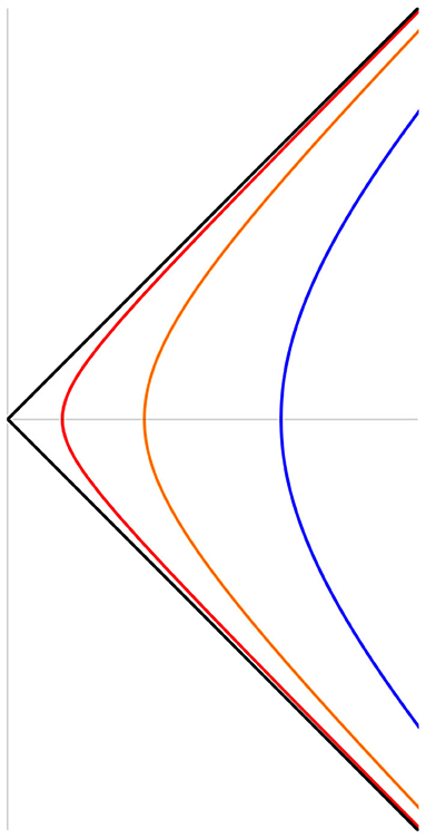
Figure 1. Rindler worldlines of observers with differing accelerations but same horizon.

2.3. Many Black Holes

Now we can consider superposing solutions for γ, to build up multi-black hole solutions as described in [36]. We will briefly review these solutions, using a slightly different notation to [36] that is more suited to our argument. Each black hole is represented by a rod of length 2m_I, I = 1..N, and acceleration is represented by a SILM as described above. We will label the rod ends at z_i, where i = 1..n and z₁ < z₂ < … If we have an array of accelerating black holes, n = 2N+1, and the SILM begins at z_n, if we have an array of (non-accelerating) black holes, then n = 2N is even. This arrangement is depicted in Figure 2.

FIGURE 2

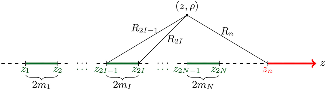
Figure 2. The source arrangement for the multi-black hole system of section 2.3. In the non-accelerating case, the point z_n, representing the start of the SILM (thick red arrow), and the SILM itself are absent; its neighboring string (dashed black) instead extends to z → ∞.

A natural generalization of previous notation is

$\begin{array}{ll}{Z}_i=z-z_i,& R_i^2=r^2+Z_i^2,\\ X_i=R_i-Z_i,& E_{ij}=R_i{R}_j+Z_i{Z}_j+r^2.& (2.15)\end{array}$

The solution for γ is simply the superposition of the general potentials from (2.7), with ν then obtained by quadrature:

$\begin{array}{l}\gamma =\frac{1}{2}{\displaystyle \sum _{i=1}^n}{(-1)}^{i+1}log\frac{X_i}{{\ell }_{\gamma }},\\ \nu =\frac{1}{4}{\displaystyle \sum _{i,j=1}^n}{(-1)}^{i+j+1}log\frac{E_{ij}}{{\ell }_{\nu }^2}+O_n\gamma .& (2.16)\end{array}$

Here, the ℓ's are integration constants that cancel only if n is even, and O_n acts as a “switch” for additional terms when n is odd:

$\begin{array}{ll}{O}_n=n-2\lfloor \frac{n}{2}\rfloor =\{\begin{array}{cc}1& n\text{ odd}\\ 0& n\text{ even}\end{array}.& (2.17)\end{array}$

As we move to the thermodynamics of the system, we will need the limit of these functions as we approach the axis, r → 0. We therefore conclude this subsection by finding the behavior of (2.16) as r → 0, and discussing the conical deficits on the axis. Noting that R_i → |Z_i| as r → 0, we see that

$\begin{array}{ll}{X}_i~|Z_i|-Z_i+\frac{r^2}{2|Z_i|}=\{\begin{array}{cc}2|Z_i|& z<z_i\\ \frac{r^2}{2Z_i}& z>z_i\end{array},& (2.18)\end{array}$

hence

$\begin{array}{l}\gamma ~\frac{1}{2}{\displaystyle \sum _{i=1}^p}{(-1)}^{i+1}log\frac{r^2}{2|Z_i|{\ell }_{\gamma }}\\ +{\displaystyle \sum _{i=p+1}^n}{(-1)}^{i+1}log\frac{2|Z_i|}{{\ell }_{\gamma }}:z\in (z_p,z_{p+1})& (2.19)\end{array}$

where p = 0 if z < z₁ leaving only the second sum, and conversely the first sum for z > z_n.

Next,

$\begin{array}{ll}{E}_{ij}~\{\begin{array}{cc}2Z_i{Z}_j& z<\text{Min}\left[z_i,z_j\right],z>\text{Max}\left[z_i,z_j\right]\\ \frac{r^2{(z_i-z_j)}^2}{2|Z_i{Z}_j|}& \text{ Min}\left[z_i,z_j\right]<z<\text{Max}\left[z_i,z_j\right]\end{array}.& (2.20)\end{array}$

Hence if we approach the axis at the Ith black hole, for which z ∈ (z_2I−1, z_2I),

$\begin{array}{l}\nu ~\frac{1}{4}{\displaystyle \sum _{i,j=1}^{2I-1}}{(-1)}^{i+j+1}log\left(\frac{2Z_i{Z}_j}{{\ell }_{\nu }^2}\right)\\ +\frac{1}{4}{\displaystyle \sum _{i,j=2I}^n}{(-1)}^{i+j+1}log\left(\frac{2Z_i{Z}_j}{{\ell }_{\nu }^2}\right)\\ +\frac{1}{2}{\displaystyle \sum _{i=1}^{2I-1}}{\displaystyle \sum _{j=2I}^n}{(-1)}^{i+j+1}log\left(\frac{r^2{(z_i-z_j)}^2}{2\left|Z_i{Z}_j\right|{\ell }_{\nu }^2}\right)+O_n\gamma .& (2.21)\end{array}$

Away from the black holes, writing ${\nu }_0=\frac{1}{2}log\left(\frac{\sqrt{2}{\ell }_{\nu }}{{\ell }_{\gamma }}\right)$, we have:

$\begin{array}{ll}\begin{array}{cc}\nu (0,z)=O_n{\nu }_0\hfill & \hfill z<z_1\\ ={\displaystyle \sum _{i=1}^{2I}}{\displaystyle \sum _{j=2I+1}^n}{(-1)}^{i+j+1}log(z_j-z_i)+O_n{\nu }_0\hfill & \hfill z_{2I}<z<z_{2I+1}\\ =O_n\left[{\displaystyle \sum _{i=1}^{n-1}}{(-1)}^{i}log(z_n-z_i)+{\nu }_0\right]\hfill & \hfill z_{2N}<z<z_n.\end{array}& (2.22)\end{array}$

Notice that z_j − z_i+1 < z_j − z_i < z_j+1 − z_i, thus ν(0, z) < ν₀ for the first string tension, and (for accelerating black holes) ν_N < ν₀.

We can now identify the conical structure on the axis. The axis will have a conical defect if the circumference of circles of proper radius Δr around it are not 2πΔr. For small r, Δr ~ e^{ν(0,z)−γ(0,z)} and the circumference is 2πre^−γ(0,z)/K, hence the deficit angle δ is

$\begin{array}{ll}\delta =2\pi {\displaystyle \underset{r\to 0}{lim}}\left[1-\frac{e^{-\nu (0,z)}}{K}\right],& (2.23)\end{array}$

which is related to the cosmic string tension via δ = 8πGμ. Equation (2.22) dictates how the deficit angle changes as we move between the black holes. The tension between the Ith and (I+1)th black hole is

$\begin{array}{ll}{\mu }_I=\frac{1}{4}\left(1-\frac{e^{-O_n{\nu }_0}}{K}{\displaystyle \prod _{i=1}^{2I}}{\displaystyle \prod _{j=2I+1}^n}{(z_j-z_i)}^{{(-1)}^{i+j}}\right).& (2.24)\end{array}$

The final black hole has μ_N as the deficit for z > z_2N,

$\begin{array}{ll}{\mu }_N=\{\begin{array}{cc}\frac{1}{4}\left(1-\frac{1}{K}\right)& n=2N\\ \frac{1}{4}\left(1-\frac{e^{-{\nu }_0}}{K}{\displaystyle {\prod }_{i=1}^N}\frac{(z_n-z_{2i-1})}{(z_n-z_{2i})}\right)& n=2N+1\end{array},& (2.25)\end{array}$

and for the incident tension, z < z₁, we have

$\begin{array}{ll}{\mu }_0=\frac{1}{4}\left(1-\frac{e^{-O_n{\nu }_0}}{K}\right).& (2.26)\end{array}$

We now see the interpretation of K. For the non-accelerating black hole array, there is an ambient tension running through the system, as the deficit outside the array (z < z₁ and z > z_2N) have the same conical deficit of

$\begin{array}{ll}{\mu }_0={\mu }_N=\frac{1}{4}\left(1-\frac{1}{K}\right).& (2.27)\end{array}$

Equation (2.22) shows that e^ν(0,z) < 1 between the black holes. Hence, if we did not insert the parameter K, instead retaining a 2π periodicity of ϕ for z < z₁ and z > z_2N, the conical singularity between any two of the black holes would be an excess δ < 0, corresponding to a negative tension “cosmic strut” as in [32]. Although one can consider such systems [20, 32, 33], we prefer to keep physical sources. We therefore take K large enough that all the conical singularities are deficits and correspond, in principle, to physical cosmic strings [14, 15]. Note, however that if K > 1, there is an ambient conical deficit through the spacetime, irrespective of whether there is acceleration.

For an accelerating black hole array, we follow the convention of [27, 41] that K measures the ambient deficit, i.e.,

$\begin{array}{ll}{\mu }_0+{\mu }_N=\frac{1}{2}\left(1-\frac{1}{K}\right).& (2.28)\end{array}$

This in turn allows us to determine ν₀:

$\begin{array}{ll}{e}^{{\nu }_0}={\left(\frac{\sqrt{2}{\ell }_{\nu }}{{\ell }_{\gamma }}\right)}^{1/2}=\frac{1}{2}\left(1+{\displaystyle \prod _{i=1}^N}\frac{(z_n-z_{2i-1})}{(z_n-z_{2i})}\right)\equiv \frac{1}{2}(1+V_n).& (2.29)\end{array}$

thus we have

$\begin{array}{ll}{\mu }_0=\frac{1}{4}\left(1-\frac{2}{(1+V_n)K}\right),{\mu }_N=\frac{1}{2}\left(1-\frac{2V_n}{(1+V_n)K}\right).& (2.30)\end{array}$

Note however that the choice of K is not unique; this one, (2.30), corresponds to the same normalization as the standard C-metric, however, if one were viewing the metric as a split cosmic string, then an alternate natural choice might be to normalize the “initial” deficit. That is, we could choose ${\mu }_0=\frac{1}{4}\left(1-\frac{1}{K}\right)$, in which case ${\mu }_N=\frac{1}{4}\left(1-\frac{V_n}{K}\right)$.

Finally, we are left with the length scale ℓ_γ, which is (only) present in an accelerating array, This parameter represents the net acceleration scale of the spacetime. We expect that for small accelerations (large z_n) this should asymptote the Rindler value ℓ_γ ~ 2z_n. Interpreting the acceleration as the overall mass of the composite black hole system divided by the overall force measured by the differential deficit, we are led to

$\begin{array}{ll}{\ell }_{\gamma }=\frac{M}{{\mu }_0-{\mu }_N}=\frac{V_n+1}{V_n-1}{\displaystyle \sum _1^N}{(-1)}^k{z}_k,& (2.31)\end{array}$

where M = ∑m_I/K is the total mass of the system (see section 3.1). We see that ℓ_γ has the required large z_n limit and a clear physical interpretation in close analogy with its pure Rindler cousin from section 2.2.

3. Thermodynamics of an Array of Black Holes

We now derive a First Law for collinear black holes with varying positive tension strings and a possible acceleration horizon, the solutions for which were presented in section 2.3.

3.1. Deriving the Thermodynamic Parameters

First we need to derive these relevant thermodynamic parameters. For the entropy of a given black hole, we compute the area of the relevant horizon

$\begin{array}{ll}{S}_I={\displaystyle \underset{r\to 0}{lim}}\frac{\pi }{2K}{\displaystyle {\int }_{z_{2I-1}}^{z_{2I}}}r{e}^{\nu -2\gamma }dz=\frac{\pi m_I}{K}{\displaystyle \underset{r\to 0}{lim}}r{e}^{\nu -2\gamma }.& (3.1)\end{array}$

For the temperature, the standard techniques apply, yielding

$\begin{array}{ll}{T}_I={\displaystyle \underset{r\to 0}{lim}}\frac{1}{2\pi }\frac{e^{2\gamma }}{r{e}^{\nu }}=\frac{m_I}{2K{S}_I}.& (3.2)\end{array}$

The limit of re^ν−2γ as we approach the axis is given by (2.19), (2.21), and using (2.29), we obtain:

$\begin{array}{l}log(r{e}^{\nu -2\gamma })\to log2+O_{n}log\left(\frac{{\ell }_{\gamma }{e}^{{\nu }_0}}{2}\right)\\ +{\displaystyle \sum _{i=1}^{2I-1}}{\displaystyle \sum _{j=2I}^n}{(-1)}^{i+j+1}log|z_j-z_i|.& (3.3)\end{array}$

The most challenging thermodynamic quantity to identify is the total mass. This is in part due to the fact that external strings which extend to infinity prevent global asymptotic flatness and thus render the ADM mass [42] ill-defined. The presence of a non-compact acceleration horizon further complicates matters. Some attempt has been made [21] to redefine ADM mass in the presence of a conical defect by calculating the mass relative to conical Minkowski space, rather than pure Minkowski as one would in the usual construction. However, such a construction gives undesirable results. In particular, one would conclude that the mass of the C-metric is vanishing. This is puzzling from the perspective of having no smooth transition to the non-accelerating black hole. It is also counter to the intuition gained from the slowly accelerating black hole in AdS, for which the mass (with an appropriately normalized time coordinate) is M_AdS = m/K. One may be confident in the AdS calculation due to the holographic correspondence.

Although one may struggle to find a useful notion of ADM mass, the existence of the ∂_t isometry means that one still has a Komar construction [43] at one's disposal. Focusing first on the non-accelerating case, Costa and Perry [20] calculated the ADM mass for a system of collinear black holes without external strings (μ₀ = μ_N = 0). One can compute the asymptotic behavior,

$\begin{array}{ll}{e}^{2\gamma }~1-\frac{2({\Sigma }_{I=1}^N{m}_I)}{\tilde{r}}+{O}({\tilde{r}}^{-2}),\nu ~{O}({\tilde{r}}^{-2}),& (3.4)\end{array}$

where $\tilde{r}$ is a suitable radial coordinate, and simply read off the mass. As discussed above, when we have an ambient conical deficit the ADM mass is undefined, but we may instead read off the Komar mass as $M=\sum _{I=1}^N{m}_I/K$.

When an acceleration horizon is present, the situation requires more explanation. We take k = ∂_t as our Killing vector field generating time translations. The normalization of k is implicit in the choice (2.31) of ℓ_γ; see the discussion given at the end of section 2. The covector associated to k is k^♭ = e^2γdt. Taking the exterior derivative and Hodge dual, we find

$\begin{array}{ll}\star d{k}^{♭}=\frac{r}{K{e}^{2\gamma }}\left[({\partial }_r{e}^{2\gamma })dz-({\partial }_z{e}^{2\gamma })dr\right]\wedge d\varphi .& (3.5)\end{array}$

The causal structure of the spacetime is now significantly more complicated than in the non-accelerating case, but there is still a well defined spatial infinity [44]. To calculate the total mass, one could, in principle, integrate this form over a two-surface there. That said, it is more instructive to use Gauss' law to rewrite the boundary integral as the sum of integrals over each black hole horizon and a bulk integration:

$\begin{array}{ll}\frac{1}{8\pi }{\displaystyle {\int }_{\infty }}\star d{k}^{♭}=\frac{1}{8\pi }{\displaystyle \sum _{I=1}^N}{\displaystyle {\int }_{{{H}}_I}}\star d{k}^{♭}+M_{\text{bulk}}.& (3.6)\end{array}$

The quantity on the left hand side is the total mass³ M. From (2.19) and (2.21), we have the relevant behavior for the integrand on the right hand side of (3.6) near the I^th horizon ${{H}}_I$,

$\begin{array}{lll}{\partial }_r{e}^{2\gamma }~\frac{r}{2\left|z_{2I+1}{z}_{2I}\right|},& e^{-2\gamma }~\frac{4\left|z_{2I+1}{z}_{2I}\right|}{r^2},& (3.7)\end{array}$

making the integrand straightforward:

$\begin{array}{ll}{\displaystyle \underset{r\to 0}{lim}}{\left[\star d{k}^{♭}\right]}_{z\in (z_{2I},z_{2I+1})}=\frac{2}{K}dz\wedge d\varphi +\dots .& (3.8)\end{array}$

Hence we conclude that the integral over ${{H}}_I$, which we interpret as the mass of an individual black hole in the array, is

$\begin{array}{ll}{M}_I\equiv \frac{1}{8\pi }{\displaystyle {\int }_{{{H}}_I}}\star d{k}^{♭}=\frac{m_I}{K}.& (3.9)\end{array}$

Finally, we note that the volume integral M_bulk vanishes, and that the strings themselves make no contribution to the above calculation.

The conclusion is that the total Komar mass is directly related to the rod lengths of compact horizons. The same result for the mass of the solitary accelerating black hole has been proposed in [28], albeit with a non-commital attitude to the normalization of k. We also observe a clear similarity with the holographically calculated mass of a slowly accelerating black hole in AdS [27].

3.2. The First Law of Thermodynamics

We now show how to derive equation (1.2), the first law of thermodynamics for an array of collinear black holes. Consider a variation to the array. The solution (2.16) describes a coupled system; any variation of one black hole will impact on all the others. Therefore, we do not expect individual First Laws for each black hole. Instead, it makes sense to consider a variation of the total mass

$\begin{array}{ll}M={\displaystyle \sum _{I=1}^N}\frac{m_I}{K},& (3.10)\end{array}$

as this is a state function of the complete system. Indeed, this is the philosophy for the First Law derived in [32]. Thus, to derive a First Law, we must compute

$\begin{array}{ll}\delta M={\displaystyle \sum _{I=1}^N}\frac{1}{K}\delta m_I-m_I\frac{\delta K}{K^2}.& (3.11)\end{array}$

We begin by computing the variation in entropies for the individual black holes:

$\begin{array}{ll}{\displaystyle \sum _{I=1}^N}{T}_I\delta S_I=\frac{1}{2}{\displaystyle \sum _{I=1}^N}\delta \left(\frac{m_I}{K}\right)+S_{\Sigma }+\frac{O_{n}M}{2}\left(\frac{\delta {\ell }_{\gamma }}{{\ell }_{\gamma }}+\delta {\nu }_0\right),& (3.12)\end{array}$

having replaced ${\ell }_{\nu }=e^{2{\nu }_0}{\ell }_{\gamma }/\sqrt{2}$, and where

$\begin{array}{l}{S}_{\Sigma }={\displaystyle \sum _{I=1}^N}\frac{m_I}{2K}{\displaystyle \sum _{i=1}^{2I-1}}{\displaystyle \sum _{j=2I}^{2N}}{(-1)}^{i+j+1}\frac{\delta (z_j-z_i)}{z_j-z_i}\\ +O_n{\displaystyle \sum _{I=1}^N}\frac{m_I}{2K}{\displaystyle \sum _{i=1}^{2I-1}}{(-1)}^i\frac{\delta (z_n-z_i)}{z_n-z_i}.& (3.13)\end{array}$

This contains part of what we need for a First Law, but has a rather messy sum!

Now we turn to the cosmic strings. We write the thermodynamic lengths for the strings as ${\lambda }_I=-e^{{\nu }_I}{L}_I$, and then vary the tensions in (2.24), (2.25), and (2.26) to obtain the contribution to the First Law coming from the tensions:

$\begin{array}{ll}-{\displaystyle \sum _{I=0}^N}{\lambda }_I\delta {\mu }_I={\displaystyle \sum _{I=0}^N}\frac{L_I\delta K}{4K^2}+O_n{\displaystyle \sum _{I=0}^N}\frac{L_I}{4K}\delta {\nu }_0+{\mu }_{\Sigma },& (3.14)\end{array}$

where

$\begin{array}{l}{\mu }_{\Sigma }={\displaystyle \sum _{I=1}^{N-1}}\frac{L_I}{4K}{\displaystyle \sum _{i=1}^{2I}}{\displaystyle \sum _{j=2I+1}^{2N}}{(-1)}^{i+j+1}\frac{\delta (z_j-z_i)}{z_j-z_i}\\ +O_n{\displaystyle \sum _{I=1}^N}\frac{L_I}{4K}{\displaystyle \sum _{i=1}^{2I}}{(-1)}^i\frac{\delta (z_n-z_i)}{z_n-z_i}.& (3.15)\end{array}$

Putting these two expressions together, we have:

$\begin{array}{l}{\displaystyle \sum _{I=1}^N}{T}_I\delta S_I-{\displaystyle \sum _{I=0}^N}{\lambda }_I\delta {\mu }_I\\ =\frac{\delta M}{2}+S_{\Sigma }+{\mu }_{\Sigma }+{\displaystyle \sum _{I=0}^N}\frac{L_I\delta K}{4K^2}+\frac{O_n}{4K}{\displaystyle \sum _{I=0}^N}(L_I+2m_I)\delta {\nu }_0\\ +2m_I\frac{\delta {\ell }_{\gamma }}{{\ell }_{\gamma }}.& (3.16)\end{array}$

First, let us deal with the sums S_Σ and μ_Σ in these expressions. Observing that m_I = (z_2I − z_2I−1)/2, we can rewrite the entropy sum as

$\begin{array}{l}{S}_{\Sigma }={\displaystyle \sum _{k=1}^{2N}}{\displaystyle \sum _{i=1}^{2\left[\frac{k+1}{2}\right]-1}}{\displaystyle \sum _{j=2\left[\frac{k+1}{2}\right]}^{2N}}\frac{{(-1)}^{i+j+k+1}}{4K}{z}_k\frac{\delta (z_j-z_i)}{z_j-z_i}\\ +\frac{O_n}{4K}{\displaystyle \sum _{k=1}^{2N}}{\displaystyle \sum _{i=1}^{2\left[\frac{k+1}{2}\right]-1}}{(-1)}^{i+k}{z}_k\frac{\delta (z_n-z_i)}{z_n-z_i}& (3.17)\end{array}$

Generalizing [32] for the thermodynamic lengths of strings in between horizons as L_I = z_2I+1 − z_2I (with the exception of L₀ and L_N – see later) gives the tension sum as

$\begin{array}{l}{\mu }_{\Sigma }={\displaystyle \sum _{k=2}^{2N-1}}{\displaystyle \sum _{i=1}^{2\left[\frac{k}{2}\right]}}{\displaystyle \sum _{j=2\left[\frac{k}{2}\right]+1}^{2N}}\frac{{(-1)}^{i+j+k}}{4K}{z}_k\frac{\delta (z_j-z_i)}{z_j-z_i}\\ +\frac{O_n}{4K}{\displaystyle \sum _{k=1}^{2N-1}}{\displaystyle \sum _{i=1}^{2\left[\frac{k}{2}\right]}}{(-1)}^{i+k+1}{z}_k\frac{\delta (z_n-z_i)}{z_n-z_i}\\ +\frac{L_N}{4K}{\displaystyle \sum _{i=1}^{2N}}{(-1)}^i\frac{\delta (z_n-z_i)}{z_n-z_i}.& (3.18)\end{array}$

We now see that many of the terms in S_Σ are canceled by terms in μ_Σ, leaving just k = 1, 2N from the entropy sum, and intermediate i, j terms from each when $2\left[\frac{k+1}{2}\right]$ differs from $2\left[\frac{k}{2}\right]+1$:

$\begin{array}{l}{S}_{\Sigma }+{\mu }_{\Sigma }\\ ={\displaystyle \sum _{j=2}^{2N}}\frac{{(-1)}^{j+1}}{4K}{z}_1\frac{\delta (z_j-z_1)}{z_j-z_1}+{\displaystyle \sum _{i=1}^{2N-1}}\frac{{(-1)}^{i+1}}{4K}{z}_{2N}\frac{\delta (z_{2N}-z_i)}{z_{2N}-z_i}\\ +{\displaystyle \sum _{k=2}^{2N-1}}\left[{\displaystyle \sum _{j=k+1}^{2N}}\frac{{(-1)}^{j+k}}{4K}{z}_k\frac{\delta (z_j-z_k)}{z_j-z_k}+{\displaystyle \sum _{i=1}^{k-1}}\frac{{(-1)}^{i+k+1}}{4K}{z}_k\frac{\delta (z_i-z_k)}{z_i-z_k}\right]\\ +\frac{O_n}{4K}\left({\displaystyle \sum _{i=1}^{2N-1}}\left[{(-1)}^i(L_N+z_{2N})-z_i\right]\frac{\delta (z_n-z_i)}{z_n-z_i}+L_N\frac{\delta (z_n-z_{2N})}{z_n-z_{2N}}\right)\\ ={\displaystyle \sum _{j=2}^{2N}}{\displaystyle \sum _{i=1}^{j-1}}\frac{{(-1)}^{i+j+1}}{4K}(\delta z_j-\delta z_i)\\ +\frac{O_n}{4K}{\displaystyle \sum _{k=1}^{2N}}{(-1)}^k(L_N+z_{2N}-z_k)\frac{\delta (z_n-z_k)}{z_n-z_k}.& (3.19)\end{array}$

We now have to identify L_N (and L₀). We write

$\begin{array}{ll}{L}_N=z_c-z_{2N},L_0=z_1-z_c& (3.20)\end{array}$

in keeping with the expressions for L_I, where z_c is a normalization, similar to that of the SILM in γ, to be determined. We can therefore reduce this combination to

$\begin{array}{l}{S}_{\Sigma }+{\mu }_{\Sigma }={\displaystyle \sum _{I=1}^N}\frac{\delta m_I}{2K}\\ +\frac{O_n}{4K}{\displaystyle \sum _{k=1}^{2N}}{(-1)}^k\left(\delta (z_n-z_k)+(z_c-z_n)\frac{\delta (z_n-z_k)}{z_n-z_k}\right)\\ ={\displaystyle \sum _{I=1}^N}\frac{\delta m_I}{2K}(1-O_n)+\frac{O_n}{4K}(z_c-z_n){\displaystyle \sum _{k=1}^{2N}}{(-1)}^k\frac{\delta (z_n-z_k)}{z_n-z_k}\\ ={\displaystyle \sum _{I=1}^N}\frac{\delta m_I}{2K}(1-O_n)-\frac{O_n}{4K}(z_c-z_n)\frac{\delta V_n}{V_n}.& (3.21)\end{array}$

Having simplified S_Σ+μ_Σ, we now turn to the rest of the putative First Law, (3.16). We note that the sum of the thermodynamic lengths can be related to the sum of the masses:

$\begin{array}{ll}{\displaystyle \sum _{I=0}^N}{L}_I={\displaystyle \sum _{I=1}^{N-1}}(z_{2I+1}-z_{2I})+L_N+L_0=-2{\displaystyle \sum _{I=1}^N}{m}_I.& (3.22)\end{array}$

Hence,

$\begin{array}{l}{\displaystyle \sum _{I=1}^N}{T}_I\delta S_I-{\displaystyle \sum _{{\mu }^{\prime }s}}{\lambda }_I\delta {\mu }_I=\frac{\delta M}{2}+{\displaystyle \sum _{I=0}^N}\frac{L_I\delta K}{4K^2}+{\displaystyle \sum _{I=1}^N}\frac{\delta m_I}{2K}\\ +\frac{O_n}{4K}\left[{\displaystyle \sum _{I=1}^N}2m_I\frac{\delta {\ell }_{\gamma }}{{\ell }_{\gamma }}-{\displaystyle \sum _{I=1}^N}2\delta m_I-(z_c-z_n)\frac{\delta V_n}{V_n}\right]\\ =\delta M+\frac{O_n}{2K}\left[m_{\text{tot}}\frac{\delta {\ell }_{\gamma }}{{\ell }_{\gamma }}-\delta m_{\text{tot}}-(z_c-z_n)\frac{\delta V_n}{2V_n}\right],& (3.23)\end{array}$

where $m_{\text{tot}}=\sum _I{m}_I$ is shorthand for the sum of the individual rod lengthscales. Thus, we have derived the First Law (1.2) for a general array of black holes, provided we identify

$\begin{array}{ll}{z}_c=z_n+\frac{2m_{\text{tot}}\delta {\ell }_{\gamma }/{\ell }_{\gamma }-2\delta m_{\text{tot}}}{\delta V_n/V_n}=z_n-\frac{4V_n{m}_{\text{tot}}}{V_n^2-1},& (3.24)\end{array}$

for the accelerating black hole. For the non-accelerating black hole, the First Law is automatically satisfied and we set L₀ = L_N = (z₁ + z_2N)/2.

4. Exploring Multi-Black Hole Spacetimes

Having derived these expressions, it is interesting to explore some sample accelerating and non-accelerating black hole arrays to gain an understanding of the interdependency of black hole entropy, and to see how the strings contribute to the thermodynamic system as well as cross-checking against known results.

4.1. Non-accelerating Arrays

We start by considering non-accelerating black holes. This includes the Schwarzschild case as a basic cross-check of our results, and the two black hole system which has already been considered in the literature [20, 32, 33].

4.1.1. Schwarzschild With a String

As discussed in section 2, the Schwarzschild solution (with an axial conical defect) has n = 2, N = 1, and z₂ − z₁ = 2m. Conventionally, we set the center of the rod at the origin so that z₂ = −z₁ = m. From (3.1) and (3.2) we find that the entropy and temperature are S = 4πm²/K and T = 1/8πm, respectively, as expected. For the cosmic string piercing the horizon, we have ${\mu }_0={\mu }_1=\frac{1}{4}\left(1-\frac{1}{K}\right)$, and λ₀ = λ₁ = m in agreement with [26].

4.1.2. Two Black Holes

The First Law for the two black hole system, with K = 1, was explored in [32]. This value of K means that there are no strings running to infinity, but instead the black holes are held apart by a negative tension strut. Nevertheless, for larger K,

$\begin{array}{ll}K\ge \frac{D^2-{\left(m_2-m_1\right)}^2}{D^2-{\left(m_1+m_2\right)}^2}& (4.1)\end{array}$

where D is the distance between the centers of the two rods, we find results harmonious with their conclusions: the First Law holds with the thermodynamic length of the defect connecting the black holes given by the worldsheet volume of the string per unit time. The thermodynamic lengths of the semi-infinite strings are now

$\begin{array}{ll}{\lambda }_0={\lambda }_2=\frac{z_4-z_1}{2}=\frac{D}{2}+\frac{m_1+m_2}{2}& (4.2)\end{array}$

i.e., the system responds to the average mass, and the length between the black holes. Note that ${\lambda }_1=-\left(z_3-z_2\right)e^{{\nu }_1}$ also has a factor of the separation that is important for consistency in varying the net conical deficit of the system. We discuss this in more detail below for three black holes.

4.1.3. Three Black Holes

The three black hole system has rods on the intervals (z₁, z₂), (z₃, z₄), and (z₅, z₆) (see Figure 3). We are interested in exploring how the locations of the sources affect entropy and tension, and how a perturbation of one black hole impacts on the others. Hence, we consider a set-up in which the two outer black holes have equal mass and spacing from the middle black hole, which is centred around the origin: z₆ − z₅ = z₂ − z₁ = 2m₀, and z₆ = −z₁ = z₀, z₄ = −z₃ = m. The entropies and tensions then become:

$\begin{array}{l}{S}_1=\frac{4\pi m_0^2}{K}\frac{(z_0+m_0)(z_0+m_0+m)}{z_0(z_0+m_0-m)}=S_3\\ S_2=\frac{4\pi m^2}{K}\frac{(z_0^2-m_0^2){(z_0+m_0+m)}^2}{z_0^2{(z_0-m_0+m)}^2}\\ {\mu }_0=\frac{1}{4}\left(1-\frac{1}{K}\right)\\ {\mu }_1=\frac{1}{4}\left(1-\frac{z_0^2(z_0^2-{(m_0-m)}^2)}{(z_0^2-m_0^2)(z_0^2-{(m_0+m)}^2)K}\right)={\mu }_2.& (4.3)\end{array}$

It is easy to see that μ₁ < μ₀. This is to be expected: in order to retain equilibrium, additional force must be applied on the outer black holes to counterbalance their attraction of the middle one.

FIGURE 3

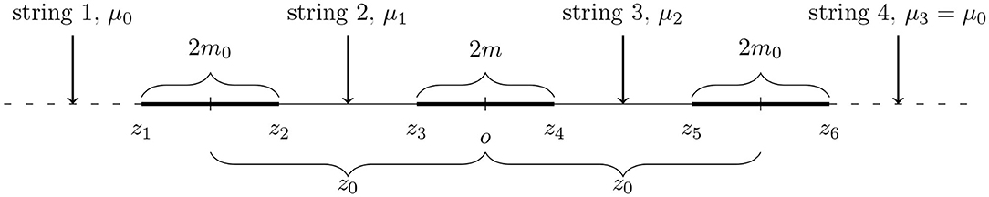
Figure 3. The source arrangement for three (non-accelerating) black holes.

For the thermodynamic lengths we have:

$\begin{array}{l}{\lambda }_0=(z_6-z_1)/2=(z_0+m_0)={\lambda }_3,\\ {\lambda }_1=-(z_0-m_0-m)\frac{(z_0^2-m_0^2)(z_0^2-{(m_0+m)}^2)}{z_0^2(z_0^2-{(m_0-m)}^2)}={\lambda }_2.& (4.4)\end{array}$

Thus, the thermodynamic length of the ambient deficit—that is, the total from both string 1 and 4—is the distance from the north pole of the topmost black hole to the south pole of the bottom-most black hole. The length associated to the intermediate strings is minus the distance between the horizons of adjacent black holes (see Figure 4).

FIGURE 4

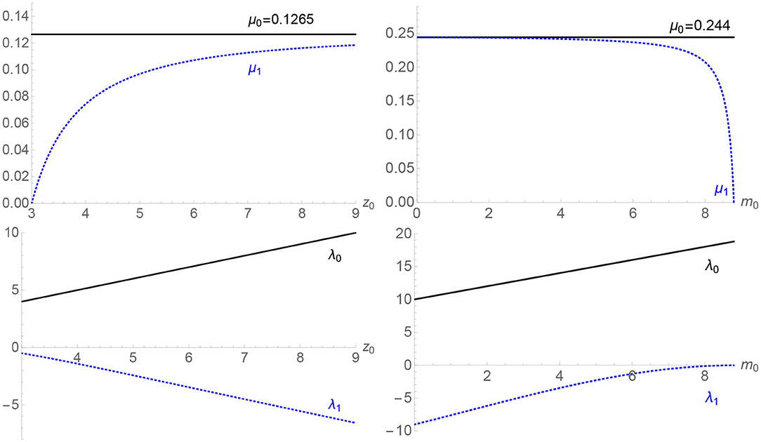
Figure 4. The variation of tensions and thermodynamic lengths of the three black hole system: (Left) for equal masses as a function of black hole separation, and (Right) for fixed black hole separation but varying the mass of the outer black hole. On the left, the tension is set by taking the minimal value consistent with zero tension between the black holes at minimum separation, z_min = 3, giving an ambient tension of 41/324. On the right the separation is set at z₀ = 10, and the outer black hole mass varies from zero to 8.8, which is very close to the merger limit of maximal tension, μ₀ ~ 0.244.

We have found an interesting phenomenon where the thermodynamic lengths of the outer strings are positive whereas those of interior strings are negative. This is puzzling from the perspective of the individual black holes. However, upon taking the system as a composite it makes sense: if we alter the overall tension, we must account for the contributions from both inner and outer cosmic strings. The negative contribution from the interior lengths then counteracts the positive contribution from the outer lengths. Explicitly, first set up the three black holes so that there is no deficit between the central and outer black holes. That is, K takes the value

$\begin{array}{ll}{K}_0=\frac{z_0^2(z_0^2-{(m_0-m)}^2)}{(z_0^2-m_0^2)(z_0^2-{(m_0+m)}^2)}.& (4.5)\end{array}$

We now “add” a cosmic string to the system by increasing K to K₀ + K₁, so that

$\begin{array}{ll}\delta {\mu }_0=\frac{K_1}{4K_0(K_0+K_1)},\delta {\mu }_1=\frac{K_1}{4(K_0+K_1)}=K_0\delta {\mu }_0.& (4.6)\end{array}$

Note that the tension of the ambient cosmic string through the whole spacetime increases from μ₀ = (1 − 1/K₀)/4 to μ₀ + δμ₀. However, the region between the black holes, which initially had no deficit, now exhibits a cosmic string with tension K₀δμ₀, i.e., a slightly greater tension than the increase in ambient string tension. Now let us look at the overall change in energy:

$\begin{array}{l}{\displaystyle \sum _{I=0}^3}{\lambda }_I\delta {\mu }_I={\lambda }_0\delta {\mu }_0+{\lambda }_1\delta {\mu }_1+{\lambda }_2\delta {\mu }_2+{\lambda }_3\delta {\mu }_3\\ =2(z_0+m_0)\frac{K_1}{4K_0(K_0+K_1)}\\ -2\frac{(z_0-m_0-m)}{K_0}\frac{K_1}{4(K_0+K_1)}\\ =\frac{(4m_0+2m)K_1}{4K_0(K_0+K_1)}.& (4.7)\end{array}$

This is the total length of string captured by the black holes multiplied by the tension. We conclude therefore that the thermodynamic lengths really do behave in concert, combining in such a way that the overall modification of tension has a sensible impact on the overall thermodynamics of the system.

Turning to the entropies, one sees that $S_2/m^2>S_1/m_0^2$. Essentially, this is saying that the inner black hole has a higher entropy in units of its mass (squared) than the outer ones. We understand this from the impact of the conical deficits: entropy is decreased in general by having a conical deficit, as part of the horizon is “cut out,” leaving a rugby, as opposed to soccer, ball shape. We would expect that the entropy of the middle black hole would be relatively higher, as the deficit running through this black hole is less than the deficit emerging from the outer poles of the outer black holes.

The picture is a little more subtle than this broad brush expectation however; the central black hole has a uniform tension, μ₁, running through it, so naively, we might expect that the entropy might be tracked by $4\pi m^2(1-4{\mu }_1)$, but in fact the entropy is higher than this. For the outer black holes, we might expect the entropy to be tracked by the average tension between the poles, but again, it is higher. Indeed, the entropy is higher even than the Schwarzschild entropy for a range of separation values z₀ (see Figure 5).

FIGURE 5

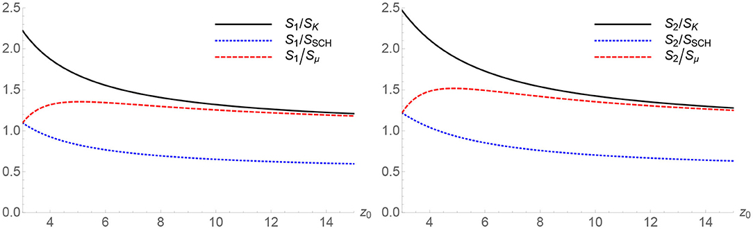
Figure 5. The entropy of the outer (left) and middle (right) black holes for equal masses as a function of black hole separation. The black holes all have unit mass, with an ambient tension of 41/324. The tension is set by taking the minimal value consistent with no strut between the black holes at minimum separation, here z_min = 3.

Similarly, we can track what happens to the entropy of one black hole as a result of changing the mass of the others. For example, keeping the central black hole at unit mass, and keeping the other two black holes at a given distance, we can see how the entropy of the central black hole

$\begin{array}{ll}{S}_{\text{central}}=\frac{4\pi }{K}\frac{(1-m^2/z_0^2){(1+m/z_0+1/z_0)}^2}{{(1-m/z_0+1/z_0)}^2}& (4.8)\end{array}$

alters as we change the mass of the outer black holes. The mass of the outer hole m₀ can range from zero to z₀ − 1, however at this point the horizons merge and to maintain a non-negative tension between the black holes we would have to have a maximal deficit of 2π. Instead, we choose a maximal mass m_max, and set K so that at the maximal mass there is no deficit between the black holes:

$\begin{array}{ll}K=K_c\equiv \frac{z_0^2(z_0^2-{(m_{\text{max}}-1)}^2)}{(z_0^2-m_{\text{max}}^2)(z_0^2-{(m_{\text{max}}+1)}^2)}.& (4.9)\end{array}$

Figure 6 shows the variation of the entropy of the central black hole for a separation z₀ = 10, and a mass range up to m_max = 8.8. This is very close to the merger limit, giving a large external tension μ₀ ~ 0.244, so a deficit angle of δ/(2π) ~ 0.977. As before, the entropy is normalized by the entropy of a single black hole in a spacetime with both this ambient deficit (S_K = 4π/K) as well as that of a black hole with a cosmic string of tension μ₁ running through (S_μ = 4π(1 − 4μ₁)).

FIGURE 6

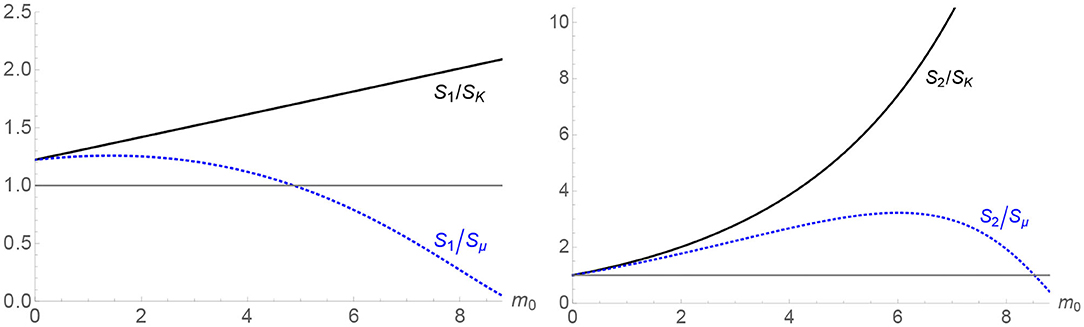
Figure 6. The entropies of the outer (left) and central (right) black holes as a function of the mass m₀ of the outer black holes. The mass of the central black hole is fixed at 1, and the outer black holes have the same mass m₀.

We now see a more nuanced behavior. Initially, at m = 0, the spacetime is precisely that of a single black hole of unit mass pierced by a cosmic string of tension μ₀ = μ₁ = (1 − 1/K)/4. As we switch on the black hole mass at z₀, μ₁ decreases, and this results in an increase in entropy, but this is over and above what we would expect simply from a drop in μ₁. This comes primarily from the m dependence in (4.8). As we increase the mass further however, while the function S₂/S_K continues to grow, the ratio S₂/S_μ, of the entropy to that of a black hole with the μ₁ cosmic string starts to drop, eventually becoming less than one. We can understand this as being a consequence of the very large deficit in the majority of the spacetime, even though locally, at the central black hole, there is no cosmic string. The outer black holes are very close (within a Schwarzschild radius) to the central black hole, thus the geometry is strongly distorted there.

4.2. Accelerating Arrays

Now let us consider accelerating black hole arrays of the type depicted in Figure 2. The main difference with the non-accelerating array is that we have chosen the parameter K to represent the ambient tension, so that the asymptotic tension in principle varies with the locations of the rod ends. The expressions for entropy, temperature, tension and thermodynamic length are readily worked out from (3.1) and (3.2), though are not particularly illuminating. However, we can intuit the general behavior as we vary the black hole masses and positions.

First, note that μ₀ > μ_N. We expect this because since the black holes are accelerating there must be an imbalance between the tension of the string coming in from infinity and that of the string exiting through the acceleration horizon. Next, as we increase the first black hole mass m₁, the first tension μ₁ will drop, as more of the pulling power of the string will be used to accelerate the increased mass. Whether the subsequent string tensions increase or decrease depends on the masses of the individual black holes: the second black hole will be attracted to the first (and third, if present) which provides an additional attractive force over and above that of the cosmic string. Typically, if the black holes are well separated relative to their size, the string tensions will cascade down in magnitude as one moves along the array, but for large black holes, this need not be the case (see the two black hole case below).

4.2.1. The C-Metric

It is worth briefly checking the C-metric results, first proposed in [28] (see also [45]). The C-metric has a single horizon and a SILM so we have n = 3 and N = 1. The metric in Weyl form is

$\begin{array}{l}d{s}^2=\frac{X_1{X}_3}{{\ell }_{\gamma }{X}_2}d{t}^2-\frac{{\ell }_{\gamma }{E}_{12}{E}_{23}}{4R_1{R}_2{R}_3{E}_{13}}{\left(\frac{z_3-z_0}{z_3-z_2}\right)}^2\left[d{r}^2+d{z}^2\right]\\ -r^2\frac{{\ell }_{\gamma }{X}_2}{X_1{X}_3}\frac{d{\varphi }^2}{K^2},& (4.10)\end{array}$

where z₀ = (z₁ + z₂)/2 is the center of the black hole rod, and we have replaced V₃ = (z₃ − z₁)/(z₂ − z₂). Here, ℓ_γ = 2(z₃ − z₀) is shown to be the reciprocal of the acceleration of a small black hole in Appendix A, where we also note the transformation between this metric and the more familiar spherical coordinates.

Turning to the thermodynamics, we compute z_c as

$\begin{array}{ll}{z}_c=z_3-\frac{(z_3-z_2)(z_3-z_1)}{(z_3-z_0)}=\frac{(z_3{z}_0-z_1{z}_2)}{(z_3-z_0)}.& (4.11)\end{array}$

Meanwhile, the entropy and thermodynamic lengths are

$\begin{array}{l}S=\frac{4\pi m^2}{K}\frac{{(z_3-z_0)}^2}{(z_3-z_2)(z_3-z_1)}\to \frac{4\pi m^2}{(1-4m^2{A}^2)}\\ {\lambda }_0=e^{{\nu }_0}(z_c-z_1)=m\frac{(z_3-z_1)}{(z_3-z_2)}\to \frac{m(1+2mA)}{(1-2mA)}\\ {\lambda }_1=e^{{\nu }_1}(z_2-z_c)=m\frac{(z_3-z_2)}{(z_3-z_1)}\to \frac{m(1-2mA)}{(1+2mA)}& (4.12)\end{array}$

in agreement with the parameters proposed in [28].

It is also straightforward to write down a Christodoulou-Ruffini-like formula [35] for the C-metric. Following [41], define a quantity Δ characterizing the average tension emerging from the black hole horizon, and a quantity C characterizing the tension differential:

$\begin{array}{l}\Delta =1-2({\mu }_0+{\mu }_1)=\frac{1}{K},\\ C=\frac{{\mu }_0-{\mu }_1}{\Delta }=\frac{z_2-z_1}{4{\ell }_{\gamma }}\to mA.& (4.13)\end{array}$

Then one finds that

$\begin{array}{ll}{M}^2=\frac{\Delta S}{4\pi }\left(1-4C^2\right).& (4.14)\end{array}$

Increasing the acceleration of the black hole while maintaining a constant ambient deficit removes energy from the black hole. This result is not as unsettling as it may first appear, as energy may be lost both across the acceleration horizon and as gravitational radiation at future infinity [46].

Electromagnetic charge Q and rotational charge J fit into the above story in a straightforward manner. By analogy with the asymptotically AdS case [41], one should expect that the Christodoulou-Ruffini formula will take the form

$\begin{array}{ll}{M}^2=\frac{\Delta S}{4\pi }\left[{\left(1+\frac{\pi Q^2}{\Delta S}\right)}^2+{\left(\frac{2\pi J}{\Delta S}\right)}^2-4C^2\right].& (4.15)\end{array}$

From the charged, rotating, (asymptotically flat) C-metric written in Boyer-Lindquist type coordinates, one may explicitly calculate the conserved charges using Komar-like integrals. This was done in [28]. One then finds that (4.15) holds only if the temporal Killing vector is normalized as it was in [28], (where the choice of normalization was made in order to make the First Law and Smarr relations hold). Since the quantities Q, J, S, Δ, and C are independent of the choice of normalization, one may interpret (4.15) as evidence that the mass proposed in [28] is the correct one.

4.2.2. Two Accelerating Black Holes

As a less trivial example, we present results for the two accelerating black hole system, first explored in [36]. We have

$\begin{array}{l}{\ell }_{\gamma }=2z_5\\ -\frac{(z_4^2-z_3^2+z_2^2-z_1^2)z_5-(z_4-z_3+z_2-z_1)(z_1{z}_3+z_2{z}_4)}{(z_4-z_3+z_2-z_1)z_5+z_1{z}_3-z_2{z}_4}\\ ~2(z_5-z_{\text{com}})+{O}\left(z_5^{-1}\right),& (4.16)\end{array}$

where $z_{\text{com}}=\frac{z_4^2-z_3^2+z_2^2-z_1^2}{2(z_4-z_3+z_2-z_1)}$ is the center of mass of the pair of black holes (this formula generalizes to any number of accelerating black holes).

Placing the two black holes at ±z_b fixes the gauge, and we can see how the string tensions and black hole entropies react to changes in black hole mass and distance to the horizon (without loss of generality we can keep z_b fixed as a choice of scale). Writing

$\begin{array}{ll}{S}_0=\frac{(m_1+m_2)(m_1+m_2+2z_b){(m_1{m}_2-z_b^2+z_5^2)}^2}{(z_5+z_b+m_1)(z_5-z_b-m_2)(z_5(m_2+m_1)+z_b(m_2-m_1))},& (4.17)\end{array}$

the entropies are

$\begin{array}{ll}\begin{array}{c}{S}_1=\frac{4\pi m_1^2}{K}\frac{S_0}{(2z_b+m_1-m_2)(z_5+z_b-m_1)},\\ S_2=\frac{4\pi m_2^2}{K}\frac{S_0}{(2z_b+m_2-m_1)(z_5-z_b+m_2)}.\end{array}& (4.18)\end{array}$

We can quickly see that if m₁ = m₂, the entropy of the first black hole will always be less than that of the second, which would be expected as the mean deficit through the first black hole is greater than that through the second. However, normalizing the entropies with respect to their reference $S_K=4\pi m_I^2/K$, we can see that the multiplicative factors in (4.18) show that both initially decrease as m₂ increases from zero before turning, although S₂/S_K shows a sharper decrease and eventually drops below S₁/S_K. Again, this behavior is easy to see from the ratios in (4.18). Figure 7 shows this behavior with varying m_I.

FIGURE 7

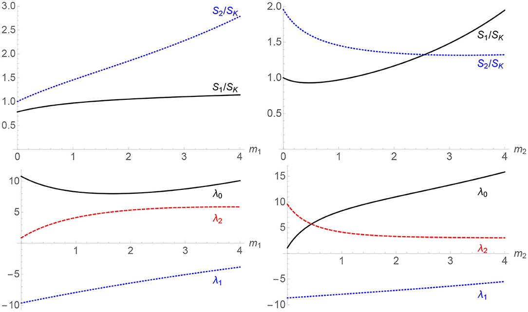
Figure 7. The variation of entropies and thermodynamic lengths as a function of mass in a two accelerating black hole set-up. The outgoing tension is fixed at μ₀ = 1/8, and the displacement of each rod from the origin at z_b = 5. One mass is fixed at unity, with the other mass varying from zero to 4. The upper plots show how the entropies, normalized by $4\pi m_I^2/K$, vary, and the lower plots the thermodynamic length. Note that K varies as m_I varies, in order to keep μ₀ fixed.

In order to compare the impact of varying the masses of the black holes and their separation, we first fix the outgoing tension at z → −∞, so that we are comparing the same conical asymptotics. Figure 7 shows the effect of varying the mass of the inner and outer black hole, respectively, on the entropies and thermodynamic lengths. In each case, we fix one of the masses at unity and vary the other. In both cases, varying the mass of the black hole closer to the acceleration horizon (m₂) causes a “crossover” behavior.

Figure 8 shows how the entropy, length (and tension) are affected by moving the black holes apart. As before, the outgoing tension is fixed at 1/8, and both black hole masses are fixed at m₁ = m₂ = 1; the acceleration horizon is at z₅ = 12. The normalized entropy of the black hole closer to the acceleration horizon increases as the black holes are moved apart, whereas the entropy of the other black hole decreases sharply. We can get a rough understanding of this by looking at the string tensions; the tension between the second black hole and the acceleration horizon drops off sharply at large separation, meaning that less of the angular direction is cut out by the deficit, thus increasing entropy. The tension between the black holes, μ₁, in contrast increases, leading to an expectation that the first entropy will decrease. While these statements are broadly true—note that we have already normalized the K factor out of the entropy, indicating that the effect of this geometry is magnified. As expected, the thermodynamic lengths exhibit a scaling with increasing separation, with the intermediate length λ₁ negative and decreasing to compensate the increase in λ₀.

FIGURE 8

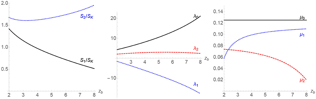
Figure 8. The variation of thermodynamic parameters for the double accelerating black hole set-up where the two black holes have equal mass m₁ = m₂ = 1 and the distance between them 2z_b is varied. The acceleration horizon is fixed at z₅ = 12.

5. Conclusions

To sum up: we have proven a thermodynamic First Law for a composite system of black holes, both accelerating and isolated. We have allowed the varying of the tensions of the cosmic strings along the axis that are necessary for maintaining the equilibrium configuration. As with the accelerating AdS black hole thermodynamics previously developed, these strings have a corresponding potential, the thermodynamic length, which has a direct specification in terms of the Weyl coordinate parameterising the axis of symmetry of the black hole array.

We have presented a range of accelerating and non-accelerating black hole systems to illustrate the various facets of the thermodynamic parameters. The main point is that the black holes form a fully composite thermodynamical system—the variation of one black hole affects all the others. We also see how the tensions and lengths in a composite system collude in such a way that the overall picture makes intuitive sense, whereas the individual black hole contributions may be less transparent.

Our findings, that the thermodynamic lengths between compact horizons is related to the proper distance along the axis, are in agreement with previous results [32, 33]. However, in our construction there are also semi-infinite strings for which this proper distance would be infinite, yet this is not what we would expect thermodynamically. The thermodynamic length represents the contribution to the enthalpy from the tension (negative pressure) of the cosmic string inside the black hole, thus should be finite. We take this into account via a renormalisation process, the z_c, similar to the renormalising of the metric coefficients.

In fact, the result for λ derived in [32], can actually be understood in terms of the covariant-phase space formalism [47], much as black hole entropy and temperature were interpreted by Wald [48] and Iyer and Wald [49]. In this construction, the idea is that, on shell, variations the action consist solely of boundary data. Taking this variation to be the action of some Killing vector field corresponding to time translation, one can find a quantity which vanishes when integrated over a Cauchy slice. Taking the variation of this quantity, and splitting the integral up into boundary pieces via Gauss' law, one obtains the First Law. The contribution from infinity gives the variation in mass and the contribution at the horizon gives TδS. When strings are present, one must also consider the contribution from a new surface: a “tube” which encases the string⁴. It is precisely this contribution which provides λδμ. From this perspective, the thermodynamic lengths calculated in [27, 28] for the AdS C-metric may be seen as renormalised worldvolumes (per unit time) of the infinite proper length strings. The sense in which the external strings are renormalised in the asymptotically flat case is less clear and would be interesting to understand.

Open questions remain as to the inclusion of electric charge. Explicit solutions to Einstein-Maxwell theory describing two electrically charged black holes connected by a conical singularity, without exterior strings, are known and have been investigated thermodynamically [32, 33]. One could, therefore, proceed as in section 3, adding exterior semi-infinite strings to the system and determining the necessary modifications to the resulting thermodynamic lengths. However, since charging the black holes destroys the linearity property present in (2.3), it is not currently known how to construct arrays containing an arbitrary number of charged objects.

While the system of many black holes is not stable, it is nonetheless interesting that it too displays sensible thermodynamic properties, further supporting the inclusion of cosmic strings in the thermodynamic picture.

Data Availability Statement

The original contributions presented in the study are included in the article/supplementary material, further inquiries can be directed to the corresponding author/s.

Author Contributions

All authors listed have made a substantial, direct and intellectual contribution to the work, and approved it for publication.

Funding

This work was supported in part by the STFC (Consolidated Grant ST/P000371/1—RG, DTG—AS), and by the Perimeter Institute for Theoretical Physics (RG). Research at Perimeter Institute is supported by the Government of Canada through the Department of Innovation, Science and Economic Development Canada and by the Province of Ontario through the Ministry of Research, Innovation and Science.

Conflict of Interest

The authors declare that the research was conducted in the absence of any commercial or financial relationships that could be construed as a potential conflict of interest.

Footnotes

1. ^The existence of arrangements of more than two aligned Kerr black holes (with or without intermediating objects) has, however, been demonstrated; see for example [39] and references therein.

2. ^We make the gauge choice to center the rod at z = 0.

3. ^There is a caveat here that we have divided through to retain only the mass of objects on one side of the acceleration horizon.

4. ^Similar ideas have been applied to thermodynamic investigations of black holes possessing Misner strings [50, 51].

References

1. Bekenstein JD. Black holes and entropy. Phys Rev D. (1973) 7:2333. doi: 10.1103/PhysRevD.7.2333

CrossRef Full Text

2. Bekenstein JD. Generalized second law of thermodynamics in black hole physics. Phys Rev D. (1974) 9:3292. doi: 10.1103/PhysRevD.9.3292

CrossRef Full Text

3. Hawking SW. Particle creation by black holes. Commun Math Phys. (1975) 43:199–220. doi: 10.1007/BF02345020

CrossRef Full Text | Google Scholar

4. Gibbons GW, Hawking SW. Action integrals and partition functions in quantum gravity. Phys Rev D. (1977) 15:2752. doi: 10.1103/PhysRevD.15.2752

CrossRef Full Text

5. Bardeen JM, Carter B, Hawking SW. The Four laws of black hole mechanics. Commun Math Phys. (1973) 31:161–70. doi: 10.1007/BF01645742

CrossRef Full Text | Google Scholar

6. Teitelboim C. The cosmological constant as a thermodynamic black hole parameter. Phys Lett. (1985) 159B:293–7. doi: 10.1016/0370-2693(85)91186-4

CrossRef Full Text | Google Scholar

7. Kastor D, Ray S, Traschen J. Enthalpy and the mechanics of AdS black holes. Class Quant Grav. (2009) 26:195011. doi: 10.1088/0264-9381/26/19/195011

CrossRef Full Text | Google Scholar

8. Dolan BP. The cosmological constant and the black hole equation of state. Class Quant Grav. (2011) 28:125020. doi: 10.1088/0264-9381/28/12/125020

CrossRef Full Text | Google Scholar

9. Dolan BP. Pressure and volume in the first law of black hole thermodynamics. Class Quant Grav. (2001) 28:235017. doi: 10.1088/0264-9381/28/23/235017

CrossRef Full Text | Google Scholar

10. Kubizňák D, Mann RB. P-V criticality of charged AdS black holes. JHEP. (2012) 1207:033. doi: 10.1007/JHEP07(2012)033

CrossRef Full Text | Google Scholar

11. Kubizňák D, Mann RB, Teo M. Black hole chemistry: thermodynamics with Lambda. Class Quant Grav. (2017) 34:063001. doi: 10.1088/1361-6382/aa5c69

CrossRef Full Text | Google Scholar

12. Israel W, Khan KA. Collinear particles and bondi dipoles in general relativity. Nuovo Cim. (1964) 33:331–44. doi: 10.1007/BF02750196

CrossRef Full Text | Google Scholar

13. Aryal M, Ford L, Vilenkin A. Cosmic strings and black holes. Phys Rev D. (1986) 34:2263. doi: 10.1103/PhysRevD.34.2263

PubMed Abstract | CrossRef Full Text | Google Scholar

14. Achucarro A, Gregory R, Kuijken K. Abelian Higgs hair for black holes. Phys Rev D. (1995) 52:5729–42. doi: 10.1103/PhysRevD.52.5729

PubMed Abstract | CrossRef Full Text | Google Scholar

15. Gregory R, Kubizňák D, Wills D. Rotating black hole hair. JHEP. (2013) 6:023. doi: 10.1007/JHEP06(2013)023

CrossRef Full Text | Google Scholar

16. Kinnersley W, Walker M. Uniformly accelerating charged mass in general relativity. Phys Rev D. (1970) 2:1359. doi: 10.1103/PhysRevD.2.1359

CrossRef Full Text | Google Scholar

17. Plebanski JF, Demianski M. Rotating, charged, and uniformly accelerating mass in general relativity. Ann Phys. (1976) 98:98–127. doi: 10.1016/0003-4916(76)90240-2

CrossRef Full Text | Google Scholar

18. Gregory R, Hindmarsh M. Smooth metrics for snapping strings. Phys Rev D. (1995) 52:5598–605. doi: 10.1103/PhysRevD.52.5598

PubMed Abstract | CrossRef Full Text | Google Scholar

19. Martinez EA, York JW Jr. Thermodynamics of black holes and cosmic strings. Phys Rev D. (1990) 42:3580–3. doi: 10.1103/PhysRevD.42.3580

PubMed Abstract | CrossRef Full Text | Google Scholar

20. Costa MS, Perry MJ. Interacting black holes. Nucl Phys B. (2000) 591:469–87. doi: 10.1016/S0550-3213(00)00577-0

CrossRef Full Text | Google Scholar

21. Dutta K, Ray S, Traschen J. Boost mass and the mechanics of accelerated black holes. Class Quant Grav. (2006) 23:335–52. doi: 10.1088/0264-9381/23/2/005

CrossRef Full Text | Google Scholar

22. Herdeiro C, Kleihaus B, Kunz J, Radu E. On the Bekenstein-Hawking area law for black objects with conical singularities. Phys Rev D. (2010) 81:064013. doi: 10.1103/PhysRevD.81.064013

CrossRef Full Text | Google Scholar

23. Bonjour F, Emparan R, Gregory R. Vortices and extreme black holes: the Question of flux expulsion. Phys Rev D. (1999) 59:084022. doi: 10.1103/PhysRevD.59.084022

CrossRef Full Text | Google Scholar

24. Papadimitriou I, Skenderis K. Thermodynamics of asymptotically locally AdS spacetimes. JHEP. (2005) 8:4. doi: 10.1088/1126-6708/2005/08/004

CrossRef Full Text

25. Appels M, Gregory R, Kubizňák D. Thermodynamics of accelerating black holes. Phys Rev Lett. (2016) 117:131303. doi: 10.1103/PhysRevLett.117.131303

PubMed Abstract | CrossRef Full Text | Google Scholar

26. Appels M, Gregory R, Kubizňák D. Black hole thermodynamics with conical defects. JHEP. (2017) 1705:116. doi: 10.1007/JHEP05(2017)116

CrossRef Full Text | Google Scholar

27. Anabalón A, Appels M, Gregory R, Kubizňák D, Mann RB, Övgün A. Holographic thermodynamics of accelerating black holes. Phys Rev D. (2018) 98:104038. doi: 10.1103/PhysRevD.98.104038

CrossRef Full Text | Google Scholar

28. Anabalón A, Gray F, Gregory R, Kubizňák D, Mann RB. Thermodynamics of charged, rotating, and accelerating black holes. JHEP. (2019) 4:096. doi: 10.1007/JHEP04(2019)096

CrossRef Full Text | Google Scholar

29. Traschen JH, Fox D. Tension perturbations of black brane space-times. Class Quant Grav. (2004) 21:289–306. doi: 10.1088/0264-9381/21/1/021

CrossRef Full Text | Google Scholar

30. Harmark T, Obers NA. General definition of gravitational tension. JHEP. (2004) 405:043. doi: 10.1088/1126-6708/2004/05/043

CrossRef Full Text | Google Scholar

31. Kastor D, Traschen J. The angular tension of black holes. Phys Rev D. (2012) 86:081501. doi: 10.1103/PhysRevD.86.081501

CrossRef Full Text | Google Scholar

32. Krtouš P, Zelnikov A. Thermodynamics of two black holes. JHEP. (2020) 02:164. doi: 10.1007/JHEP02(2020)164

CrossRef Full Text | Google Scholar

33. Ramírez-Valdez CJ, García-Compeán H, Manko VS. Thermodynamics of two aligned Kerr black holes. Phys Rev D. (2020) 102:024084. doi: 10.1103/PhysRevD.102.024084

CrossRef Full Text | Google Scholar

34. Weyl H. Zur Gravitationstheorie. Ann Phys. (1917) 359:117–45. doi: 10.1002/andp.19173591804

CrossRef Full Text | Google Scholar

35. Christodoulou D, Ruffini R. Reversible transformations of a charged black hole. Phys Rev D. (1971) 4:3552. doi: 10.1103/PhysRevD.4.3552

CrossRef Full Text | Google Scholar

36. Dowker HF, Thambyahpillai SN. Many accelerating black holes. Class Quant Grav. (2003) 20:127–36. doi: 10.1088/0264-9381/20/1/310

CrossRef Full Text | Google Scholar

37. Munguia C. Unequal binary configurations of interacting Kerr black holes. Phys Lett B. (2018) 786:466–71. doi: 10.1016/j.physletb.2018.10.037

CrossRef Full Text | Google Scholar

38. Manko VS, Ruiz E. Metric for two arbitrary Kerr sources. Phys Lett B. (2019) 794:36–40. doi: 10.1016/j.physletb.2019.05.027

CrossRef Full Text | Google Scholar

39. Manko VS, Ruiz E, Manko OV. Is equillibrium of aligned Kerr black holes possible? Phys Rev Lett. (2000) 85:5504. doi: 10.1103/PhysRevLett.85.5504

PubMed Abstract | CrossRef Full Text | Google Scholar

40. Emparan R, Reall HS. Generalized Weyl solutions. Phys Rev D. (2002) 65:084025. doi: 10.1103/PhysRevD.65.084025

CrossRef Full Text | Google Scholar

41. Gregory R, Scoins A. Accelerating black hole chemistry. Phys Lett B. (2019) 796:191–5. doi: 10.1016/j.physletb.2019.06.071

CrossRef Full Text | Google Scholar

42. Arnowitt R, Deser S, Misner C. Dynamical structure and definition of energy in general relativity. Phys Rev. (1959) 116:1322–30. doi: 10.1103/PhysRev.116.1322

CrossRef Full Text | Google Scholar

43. Komar A. Positive-definite energy density and global consequences for general relativity. Phys Rev. (1963) 129:1873-6. doi: 10.1103/PhysRev.129.1873

CrossRef Full Text | Google Scholar

44. Grffiths JB, Krtouš P, Podolsky J. Interpreting the C-metric. Class Quant Grav. (2006) 23:6745–66. doi: 10.1088/0264-9381/23/23/008

CrossRef Full Text | Google Scholar

45. Ball A, Miller N. Accelerating black hole thermodynamics with boost time. [arXiv:2008.03682 [hep-th]].

Google Scholar

46. Podolsky J, Ortaggio M, Krtous P. Radiation from accelerated black holes in an anti-de Sitter universe. Phys Rev D. (2003) 68:124004. doi: 10.1103/PhysRevD.68.124004

CrossRef Full Text | Google Scholar

47. Harlow D, Wu J. Covariant phase space with boundaries. JHEP. (2020) 10:146. doi: 10.1007/JHEP10(2020)146

CrossRef Full Text | Google Scholar

48. Wald RM. Black hole entropy is the Noether charge. Phys.Rev D. (1993) 48:R3427–31. doi: 10.1103/PhysRevD.48.R3427

PubMed Abstract | CrossRef Full Text | Google Scholar

49. Iyer V, Wald RM. Some properties of Noether charge and a proposal for dynamical black hole entropy. Phys Rev D. (1994) 50:846–64. doi: 10.1103/PhysRevD.50.846

PubMed Abstract | CrossRef Full Text | Google Scholar

50. Bordo AB, Gray F, Hennigar R, Kubizňák D Misner gravitational charges and variable string strengths. Class Quant Grav. (2019) 36:194001. doi: 10.1088/1361-6382/ab3d4d

CrossRef Full Text | Google Scholar

51. Bordo AB, Gray F, Hennigar R, Kubizňák D. The first law for rotating NUTs. Phys Lett B. (2019) 798:134972. doi: 10.1016/j.physletb.2019.134972

CrossRef Full Text | Google Scholar

52. Hong K, Teo E. A new form of the C metric. Class Quant Grav. (2003) 20:3269. doi: 10.1088/0264-9381/20/14/321

CrossRef Full Text | Google Scholar

Appendix A

Coordinate Systems for the C-Metric

We collect the transformation formulae between the standard C-metric (expressed in Hong-Teo form [52]) and the Weyl form of section 2. The C-metric in Weyl form is

$\begin{array}{l}d{s}^2=\frac{X_1{X}_3}{{\ell }_{\gamma }{X}_2}d{t}^2-\frac{{\ell }_{\gamma }{E}_{12}{E}_{23}}{4R_1{R}_2{R}_3{E}_{13}}{\left(\frac{V_3+1}{2}\right)}^2\left[d{r}^2+d{z}^2\right]\\ -r^2\frac{{\ell }_{\gamma }{X}_2}{X_1{X}_3}\frac{d{\varphi }^2}{K^2},& (\mathrm{A1})\end{array}$

where ℓ_γ = z₃ − z₀ = z₃ − (z₁ + z₂)/2 is the z-distance to the center of the black hole rod.

Now let m = (z₂ − z₁)/2 and A = 1/ℓ_γ. Define

$\begin{array}{l}r=\stackrel{-}{r}sin\theta \frac{\sqrt{f(\stackrel{-}{r})g(\theta )}}{{(1+A\stackrel{-}{r}cos\theta )}^2},\\ z-z_0=\stackrel{-}{r}\frac{(A\stackrel{-}{r}+cos\theta )(1-m/\stackrel{-}{r}+mAcos\theta )}{{(1+A\stackrel{-}{r}cos\theta )}^2},& (\mathrm{A2})\end{array}$

where

$\begin{array}{ll}f(R)=(1-A^2{\stackrel{-}{r}}^2)\left(1-\frac{2m}{\stackrel{-}{r}}\right),g(\theta )=(1+2mAcos\theta ).& (\mathrm{A3})\end{array}$

Then the Weyl metric (4.1) transforms to the C-metric in Hong-Teo coords [52], rather than the standard Kinnersley-Walker coordinates discussed in [36]:

$\begin{array}{l}d{s}^2=\frac{1}{{(1+A\overline{r}\cos \theta )}^2}[\overline{f}(\overline{r})d{t}^2-\frac{d{\overline{r}}^2}{\overline{f}(\overline{r})}\\ -{\overline{r}}^2\left(\frac{d{\theta }^2}{\overline{g}(\theta )}-\overline{g}(\theta ){\sin }^2\theta d{\varphi }^2\right)].& (\mathrm{A4})\end{array}$

Here we see the direct interpretation of ℓ_γ as the acceleration length scale; for small m, A = 1/ℓ_γ corresponds to the magnitude of the four-acceleration of the black hole [44].